Submitted:
18 September 2025
Posted:
19 September 2025
You are already at the latest version
Abstract
In seismic data processing, noise not only affects velocity analysis and seismic migration, but also cause potential risks in post‐stack processing because of the artifacts. The singular value decomposition (SVD) method based on time domain and frequency domain is effective for noise suppression, but it is very sensitive to singular value selection. This paper proposes the adaptive SVD denoising in both time and frequency domains (ASTF) method with three steps. Firstly, two Hankel matrices are constructed in the time domain and frequency domain respectively. Secondly, the parameters of the reconstruction matrix are adaptively selected base on the singular value second‐order difference spectrum. Finally, the weights of these two matrices are learned through ternary search. Experiments were carried out on synthetic data and field data to prove the effectiveness of ASTF. The results show that this method can effectively suppress noise.
Keywords:
adaptive
; denoising
; fusion
; seismic data
; singular value decomposition (SVD)
1. Introduction
Determining accurate exploration locations has always been a common demand in the oil and gas industry. People need clear underground information. However, the actual seismic data collected on site often contains a variety of noises [1]. Random noise is one of the most common interferences. Its existence may interfere with data processing steps such as static correction, velocity analysis and superposition [2,3]. Therefore, suppressing the noise is a basic and important work in seismic data processing.
Various methods have been developed to suppress random noise. According to the difference of effective signal and noise spatial distribution, noise can be located and suppressed [4,5]. Methods such as continuous wavelet transform [6,7], curvelet transform, empirical mode decomposition (EMD) and singular value decomposition (SVD) are widely used. The improved wavelet transform can find the local features of the target signal [8] in the time-frequency domain. However, a series of extended methods based on wavelet transform are not ideal for seismic data with complex events. Curvelet transform with multi-directional and multi-scale characteristics can meet this challenge well. It has achieved good results in suppressing random noise in 3D seismic data [9]. The improved two-dimensional discrete curvelet transform is more flexible for the adjustment of scale and angle threshold [10].
Empirical mode decomposition (EMD) has a good denoising ability [11]. The advantage of EMD is that the de-composition is fully automatic. It means that there is no need to set predefined parameters before decomposition [12]. However, EMD is based on experience, so it lacks theoretical foundation based on mathematical physics. It is also prone to aliasing of modal components, so that the accuracy of the calculation results is not high.
Singular value decomposition (SVD) is also used for denoising due to its strong versatility and low matrix requirements [13,14]. The disadvantage of SVD denoising [15,16] is that it is difficult to meet the accuracy and generalization. Local SVD combines the advantages of f-x deconvolution, which can enhance weak events to remove background noise [17]. Due to the statistical characteristics of different domains, SVD can also be used in the frequency domain. Combined with the projection to convex set method, matrix decomposition is performed in the frequency domain [18]. This method can simultaneously realize the denoising and interpolation of seismic data. SVD is introduced into the non-downsampled shear wave transform coefficients [19,20], which can analyze seismic data well [21]. Single-channel SVD and amplitude ratio are introduced to improve the signal-to-noise ratio (SNR) [22], but the calculation efficiency is not ideal. In ordinary singular spectrum analysis methods, adaptive value selection can reduce the time cost of value selection [23]. The difference between effective signal and noise propagation direction can also be used to distinguish noise. Such as polarization filtering, randon transform [24], predictive de-convolution filtering and other methods.
In this paper, we propose an adaptive SVD denoising method in the time domain and frequency domain (ASTF). Figure 1 illustrates the overall structure of the method. First, the Hankel matrices are formed in the time and frequency domain for SVD respectively. The singular values are adaptively selected according to the second-order difference spectrums of singular values to reconstruct the matrices. Then the two matrices are restored to single-channel data. They are assigned initial weights respectively. Weights are updated iteratively through ternary search. When the peak signal-to-noise ratio (PSNR) of the fusion result reaches the maximum, the iteration is stopped. Finally, the processing results of the two domains are added according to the output weight.
The ASTF method has two main advantages. On the one hand, it benefits from the different advantages of distinguishing signal and noise in the time and frequency domain. Faced with different seismic data, this method can effectively suppress random noise. On.
The other hand, ASTF does not require manual selection of singular values. The effectiveness of the processing results is properly guaranteed
Experiments were conducted on the synthetic datasets and field seismic dataset. We compared ASTF with Experiments were conducted on the synthetic datasets and field seismic dataset. We compared ASTF with three effective methods, including damped multi-channel singular spectrum analysis (DMSSA) [25], empirical mode decomposition (EMD) [26], and space-varying median filter (SVMF) [27]. The results show that our method is more effective.
2. Theory
2.1. SVD Denoising
Assuming that the matrix contains seismic signal and noise, it is expressed as:
where represents pure signal and represents noise. We perform SVD on as:
where is an orthogonal matrix composed of eigenvectors NNT, is an orthogonal matrix composed of eigenvectors NTN, Σ is a diagonal matrix composed of singular values in descending order. The first 10% or even 1% of the singular values of Σ can contain more than 90% of the energy information of N [28]. In other words, small singular values mean that their contribution to the effective signal is small.
N = X + D,
N = UΣVT,
Assuming that r is the rank of N, the effective rank of the signal matrix X is r′(r′< r). The best estimate of X can be obtained when the r′ largest singular values of N (σ1 > σ2 > ⋯> σr′) are selected to reconstruct the matrix. The discarded singular values represent the information in the noise matrix D.
2.2. Frequency Domain SVD Denoising
The seismic data N is Fourier transformed to obtain frequency domain data Nf. A certain characteristic frequency of m seismic traces is extracted to form an array (f1, f2, …, fm) to construct a Hankel matrix Hf, which can be expressed as:
where l = ⌊ ⌋ + 1. The elements on the anti-diagonal line of the matrix are the same.
If the seismic data contains k linear events without noise, the rank of the corresponding Hankel matrix is k. When the random noise in the seismic data increases, k also increases. SVD can be used to reduce the rank of the matrix to suppress random noise. Similarly, if there are missing seismic events, the corresponding column value in the matrix is 0. The corresponding frequency domain sample value is still 0, when converted to the f-x domain. k will increase if the number of zero-valued samples in the Hankel matrix increases. A low-rank matrix similar to the original matrix without missing traces can be obtained, when the Hankel matrix is reduced by SVD. It is transformed into frequency domain data. Then it performs the inverse Fourier transform to obtain the denoising result.
2.3. Adaptive Selection of Singular Values
In actual reconstruction, the selection of the singular values depend on the correlation of the effective signal. Singular values are usually artificially selected in traditional SVD methods. If these subjective methods are applied, it is difficult to guarantee the effectiveness of the experimental results. In order to meet this challenge, we propose to adaptively select singular values.
In the time domain, we convert the single-channel seismic data into a Hankel matrix Ht. Then the singular value matrix Σ is obtained by performing SVD on Ht. Σ is a diagonal matrix composed of singular values σx in descending order:
where r is the rank of matrix Σ, the singular value of the matrix satisfies σ1 ≥σ2 ≥⋯≥σr ≥0. The effective signal can be regarded as a series of coherent linear events. Random noise is messy because of its complexity. The decay speed of the singular value is from fast to slow in the Σ. The values of the fast decay part are highly correlated with the coherent information of the Hankel matrix. They represent effective signals with great energy. The values of the slow decay part mainly correspond to the weakly correlated random noise. According to the singular value second-order difference spectrum, we select the singular value corresponding to the effective signal. The first difference spectrum B of Σ is:
Second-order difference spectrum S of Σ is:
Because the decay speed of singular value changes from fast to slow. The critical value of fast and slow decay speed is the key to selecting singular value. S does not absolutely change from large to small, how to find the critical value is very important. We propose to apply a sliding time window method to find it. The threshold for judging whether it is a critical value is set as a constant percentage of the average value in the initial time window. With such a parameterization, it will stop searching as soon as the average value of the sliding window is less than the threshold. An advantage of this method is that it is actually a data-driven way to tune the parameter. It is worth noting that the reconstructed matrix is often not a Hankel matrix, which does not meet our expectations. This problem can be solved by a diagonal averaging method [14].
2.4. Adaptive Weight Fusion
Time domain SVD methods have a good denoising effect when they are directly applied on the horizontal events. But if the events are tilted or bent, they need to add cumbersome and complicated corrections. Frequency domain SVD methods can usually overcome these limitations. They avoid assuming that the events of signals are horizontal [29]. When the frequency bandwidth of the signal is wide, however, frequency domain SVD methods will also attenuate part of the signal when suppressing random noise. We propose to adaptively fusing the denoised results in the time domain and frequency domain. It combines the advantages of time domain and frequency domain, which is described in this subsection.
The denoised results in the time domain and frequency domain are assigned initial weights for fusion. The fused matrix TFN can be expressed as:
where ω ∈ [0, 1] is the weight of the time domain denoised matrix, TN is the denoised matrix in the time domain, FN is the denoised matrix in the frequency domain. In the experiment, we discovered that the influence of ω on the peak signal-to-noise ratio (PSNR) of the final result is a convex function, as shown in Figure 2.
TFN = ωTN + (1 −ω)FN,
We use ternary search to iteratively update ω and stop the iteration when PSNR reaches its maximum value:
where
where n represents the total number of samples of the seismic data, represents the cth sample of the denoised data, represents the cth sample of the clean data.
3. Experiments
In this section, synthetic datasets with simulated Gaussian-type noise is used to evaluate how effective ASTF is. We also use a field seismic dataset to illustrate the performance of the proposed method in practice. On the synthetic datasets, we utilize the widely used PSNR metric.
3.1. Adaptive Weight Fusion
This subsection introduces four synthetic datasets and a field seismic dataset used in the experiment. The four synthetic seismic datasets are generated by changing seismic wave speed, stratum and other conditions. Table 1 lists shot points, traces, samples, sampling intervals and source information of these datasets.
3.2. Synthetic Data
In this subsection, we show the denoising performance of our method on synthetic datasets. In order to verify the feasibility and effectiveness of our method, we compared the other three methods on four synthetic datasets with three noise levels (SNR = 1dB, 3dB and 5dB). The results show that our method has obvious denoising effect and can retain most of the effective signals. We first use single-channel seismic data to illustrate the method. Figure 3 shows a clean seismic trace and a noisy data by adding some random noise, the SNR of which is 1dB.
Figure 4 shows the denoising effects of DMSSA, EMD, SVMF and ASTF. Although four methods have achieved obvious results on the noisy data in Figure 3, EMD and SVMF seem to have strong residual noise. ASTF suppresses more noise and its result is relatively smooth. Figure 5 plots the added Gaussian noise and the noise of four different noise suppression methods. EMD and SVMF are less effective in suppressing noise than the other two methods. DMSSA damages a lot of effective signals while suppressing more noise. When ASTF suppresses more noise, it can retain more effective signals.
Table 2 shows the comparison results of the four methods on four complete synthetic datasets with three noise levels. The highest PSNR is indicated in bold. The results can show that ASTF performs well, especially when the signal-to-noise ratio is low, it is obviously better than other methods. Note that for synthetic data, we define the best performance by obtaining the highest PSNR, whereas for field data, the best performance is defined visually.
Figure 6 shows the denoised results in the time domain and frequency domain before fusion. Figure 7 shows the noise suppressed in the time domain and frequency domain respectively. It can be seen from Figure 6 and Figure 7 that both time domain and frequency domain processing can suppress noise. The effective signal processed in the time domain is not smooth enough. Part of the effective signal is lost when processed in the frequency domain. The denoised results of the two domains are fused according to a certain weight, which can well take into account the preservation of the signal and the suppression of the noise.
3.3. Field Data
This subsection introduces the comparison between ASTF and three effective methods (including DMSSA, EMD and SVMF) on a field dataset. Table 1 and Figure 8a show the information of the dataset. The seismic events are damaged to a certain extent below the first arrival. Figure 8b shows the denoised result of ASTF. It can be seen from this that ASFT makes the seismic event clear, and it effectively suppresses the noise.
In order to observe more clearly, we zoom in on the area framed by the black rectangle in Figure 8a,b, and compared the denoising effect with the other three methods. Figure 9a–e show part of the field data and the denoised results of DMSSA, EMD, SVMF and ASTF. The waveform of the signal is smooth if there is no noise. Figure 9a shows that the events are interfered by noise. Compared with the other three results, our method has the smoothest events after denoising. Compared with the other three results, our method has the smoothest event after denoising. The effect can be particularly shown from the lower right corner area of these figures.
Figure 10 plots the noise comparison of four different noise suppression methods. It can be seen that the EMD and SVMF methods are less effective in suppressing noise than the other two methods. DMSSA and EMD lose some effective signals. ASTF achieved a good denoising effect while not obviously attenuating the effective signals.

4. Conclusions
Field seismic data often contains a lot of random noise, which sets high demands for signal enhancement. We propose a denoising method in which the time domain and frequency domain adaptive SVD denoising results are fused. It uses a data-driven model to adaptively select the singular values of the reconstruction matrix. This reduces the time cost of selection and provides an appropriate guarantee for a good denoising effect. Due to the limitations of single-domain processing, the suppressed noise may not be ideal. This fusion method can combine their advantages well to restore a smooth effective signal. This method is compared with DMSSA, EMD and SVMF. Experimental results show that it can obtain the highest peak signal-to-noise ratio. In addition, the experimental results also show that it can effectively restore smooth effective signals without obviously attenuating the signal energy. In the field of image denoising, scholars also use other matrix decomposition methods to suppress noise. Exploring how image denoising migrates to seismic data denoising will be our future work.
References
- Wang H, Cao S, Jiang K, Wang H, Zhang Q. Seismic data denoising for complex structure using BM3D and local similarity. Journal of Applied Geophysics 2019, 170, 103759. https://www.sciencedirect.com/science/article/pii/S0926985119300114.
- Chen, Wei. Random noise reduction using a hybrid method based on ensemble empirical mode decomposition. Journal of Seismic Exploration 2017 06;26:227–249.
- Feng Z. Seismic random noise attenuation using effective and efficient dictionary learning. Journal of Applied Geophysics 2021;186:104258. https://www.sciencedirect.com/science/article/pii/S0926985121000057.
- Han J, van der Baan M. Empirical mode decomposition for seismic time-frequency analysis. Geophysics 2013 02;78(2):O9–O19. [CrossRef]
- Liu J, Marfurt K. Instantaneous spectral attributes to detect channels. Geophysics 2007 03;72. [CrossRef]
- Shan H, Ma J, Yang H. Comparisons of wavelets, contourlets and curvelets in seismic denoising. Journal of Applied Geophysics 2009;69(2):103–115. https://www.sciencedirect.com/science/article/pii/S0926985109001050.
- Anvari R, Nazari Siahsar MA, Gholtashee S, Roshandel Kahoo A, Mohammadi M. Seismic Random Noise Attenuation Us-ing Synchrosqueezed Wavelet Transform and Low-Rank Signal Matrix Approximation. IEEE Transactions on Geoscience and Remote Sensing 2017 11;55:6574–6581. [CrossRef]
- Morlet J. Wave propagation and sampling theory. Geophysics 1982 01;47:203–236. [CrossRef]
- Neelamani R, Baumstein AI, Gillard DG, Hadidi MT, Soroka WL. Coherent and random noise attenuation using the curvelet transform. The Leading Edge 2008 02;27(2):240–248. [CrossRef]
- Górszczyk A, Malinowski M, Bellefleur G. Enhancing 3D post-stack seismic data acquired in hardrock environment using 2D curvelet transform. Geophysical Prospecting 2015 03;63:903–918. [CrossRef]
- Chen Y. Dip-separated structural filtering using seislet transform and adaptive empirical mode decomposition based dip filter. Geophysical Journal International 2016;206(1):457–469. [CrossRef]
- Lv H. Noise suppression of microseismic data based on a fast singular value decomposition algorithm. Journal of Applied Geophysics 2019;170:103831. https://www.sciencedirect.com/science/article/pii/S0926985119302587.
- Gerbrands JJ. On the relationships between SVD, KLT and PCA. Pattern Recognition 1981;14(1):375–381. https: //www.sciencedirect.com/science/article/pii/0031320381900820, 1980 Conference on Pattern Recognition.
- Golyandina N, Nekrutkin V, Zhigljavsky AA. Analysis of time series structure: SSA and related techniques. Chapman & Hall/CRC 2001;p. 28–29. [CrossRef]
- G T, S CSG. Tube wave suppression in high frequency mine seismic data by singular value decomposition. Exploration Geophysics 1995;26:512–517. [CrossRef]
- LP S, SY Z. Singular value decomposition-based reconstruction algorithm for seismic traveltime tomography. IEEE Trans Image Process 1999;8:1152–4. [CrossRef]
- Maïza B, der Baan Mirko V. Local singular value decomposition for signal enhancement of seismic data. Geophysics 2007 02;72(2):V59–V65. [CrossRef]
- Ma J, Wang J, Liu G. Seismic data noise attenuation and interpolation using singular value decomposition in frequency domain. Geophysical Prospecting for Petroleum 2016;55:205–213.
- Time-frequency denoising of microseismic data, vol. All Days of SEG International Exposition and Annual Meeting; 2016, sEG-2016-13681108. [CrossRef]
- Zhao H, Li Y, Zhang C. SNR Enhancement for Downhole Microseismic Data Using CSST. IEEE Geoscience and Remote Sensing Letters 2016;13(8):1139–1143. [CrossRef]
- Liang X, Li Y, Zhang C. Noise suppression for microseismic data by non-subsampled shearlet transform based on singular value decomposition. Geophysical Prospecting 2018;66(5):894–903. https://onlinelibrary.wiley.com/doi/abs/ 10.1111/1365-2478.12576.
- Hu Y, Huang J, Tian Z, Pan S. Ground microseismic data denoising based on single-channel singular value decompose- tion and amplitude ratio. Geophysical Prospecting for Petroleum 2019;58:47–56+66.
- Lari HH, Naghizadeh M, Sacchi MD, Gholami A. Adaptive singular spectrum analysis for seismic denoising and interpo-lation. GEOPHYSICS 2019;84(2):V133–V142. [CrossRef]
- Sabbione J, Velis D, Sacchi M. Microseismic data denoising via an apex-shifted hyperbolic Radon transform; 2013. p. 2155–2161.
- Chen Y, Zhang D, Jin Z, Chen X, Zu S, Huang W, et al. Simultaneous denoising and reconstruction of 5-D seismic data via damped rank-reduction method. Geophysical Journal International 2016;206(3):1695–1717. [CrossRef]
- Chen Y, Fomel S. EMD-seislet transform. GEOPHYSICS 2018;83(1):A27–A32. [CrossRef]
- Chen Y, Zu S, Wang Y, Chen X. Deblending of simultaneous source data using a structure-oriented space-varying me dian filter. Geophysical Journal International 2019 02;216:1214–1232. [CrossRef]
- Kalman, Dan. A singularly valuable decomposition: The SVD of a matrix. College Mathematics Journal 1996;27(1):2–23.
- Trickett S. F-xy Cadzow noise suppression. Seg Technical Program Expanded Abstracts 2008 01;27:2586–2590.s. [CrossRef]
Figure 1.
The overall structure of ASTF. It is divided into upper and lower parts. The upper part is time domain adaptive SVD processing, which converts noisy data N into Hankel matrix Ht for SVD. Then the corresponding singular values in the red box are selected to reconstruct the matrix Ht′ according to the singular value second-order difference spectrum. Finally, the time domain denoised data TN is obtained. The lower part is frequency domain adaptive SVD, which converts N into frequency domain data Nf. Hf, Hf′ and FN are similar to Ht, Ht′ and TN in time domain processing. The final denoised result TFN is obtained by fusing TN and FN..
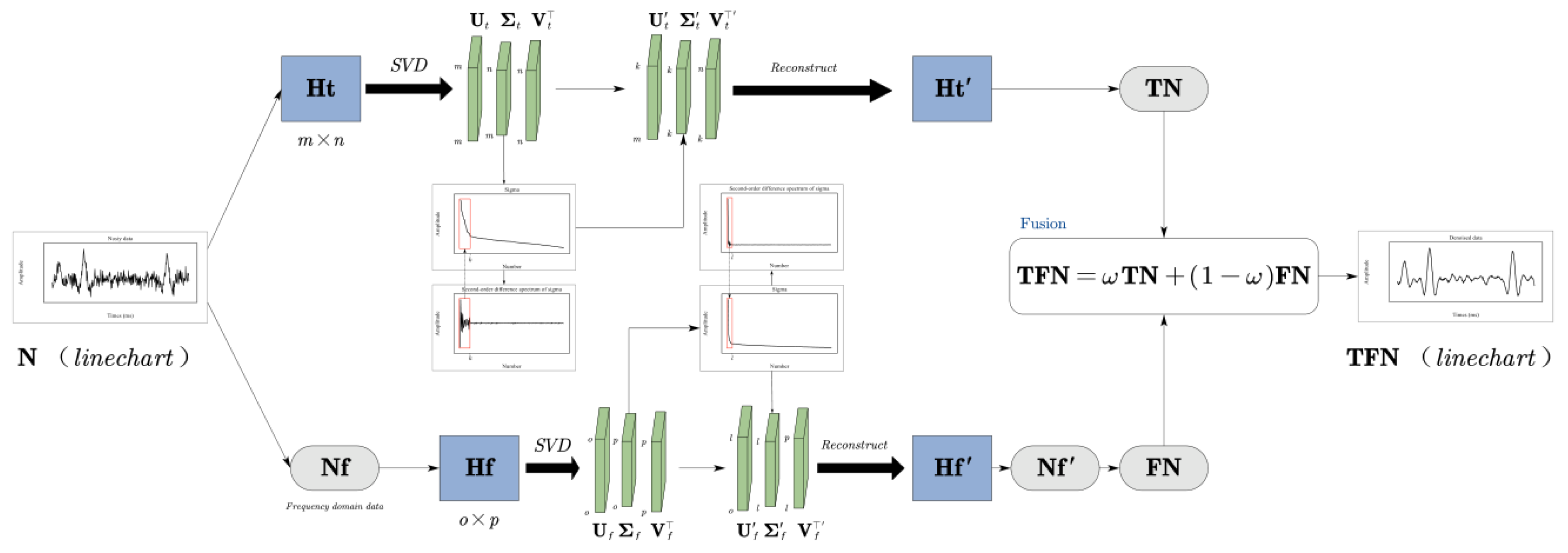
Figure 2.
The influence of ω on the PSNR.
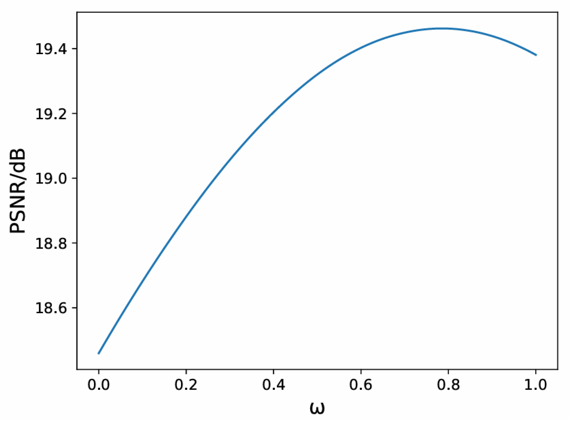
Figure 3.
Synthetic example. (a) is clean synthetic data, and (b) is noisy synthetic data with SNR = 1dB.
Figure 3.
Synthetic example. (a) is clean synthetic data, and (b) is noisy synthetic data with SNR = 1dB.
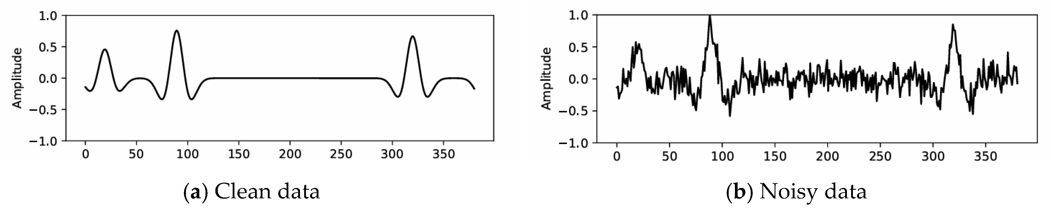
Figure 4.
Synthetic example. (a) is clean data, (b) is the denoised result of DMSSA, (c) is the denoised result of EMD, (d) is the denoised result of SVMF, and (e) is the denoised result of ASTF.
Figure 4.
Synthetic example. (a) is clean data, (b) is the denoised result of DMSSA, (c) is the denoised result of EMD, (d) is the denoised result of SVMF, and (e) is the denoised result of ASTF.
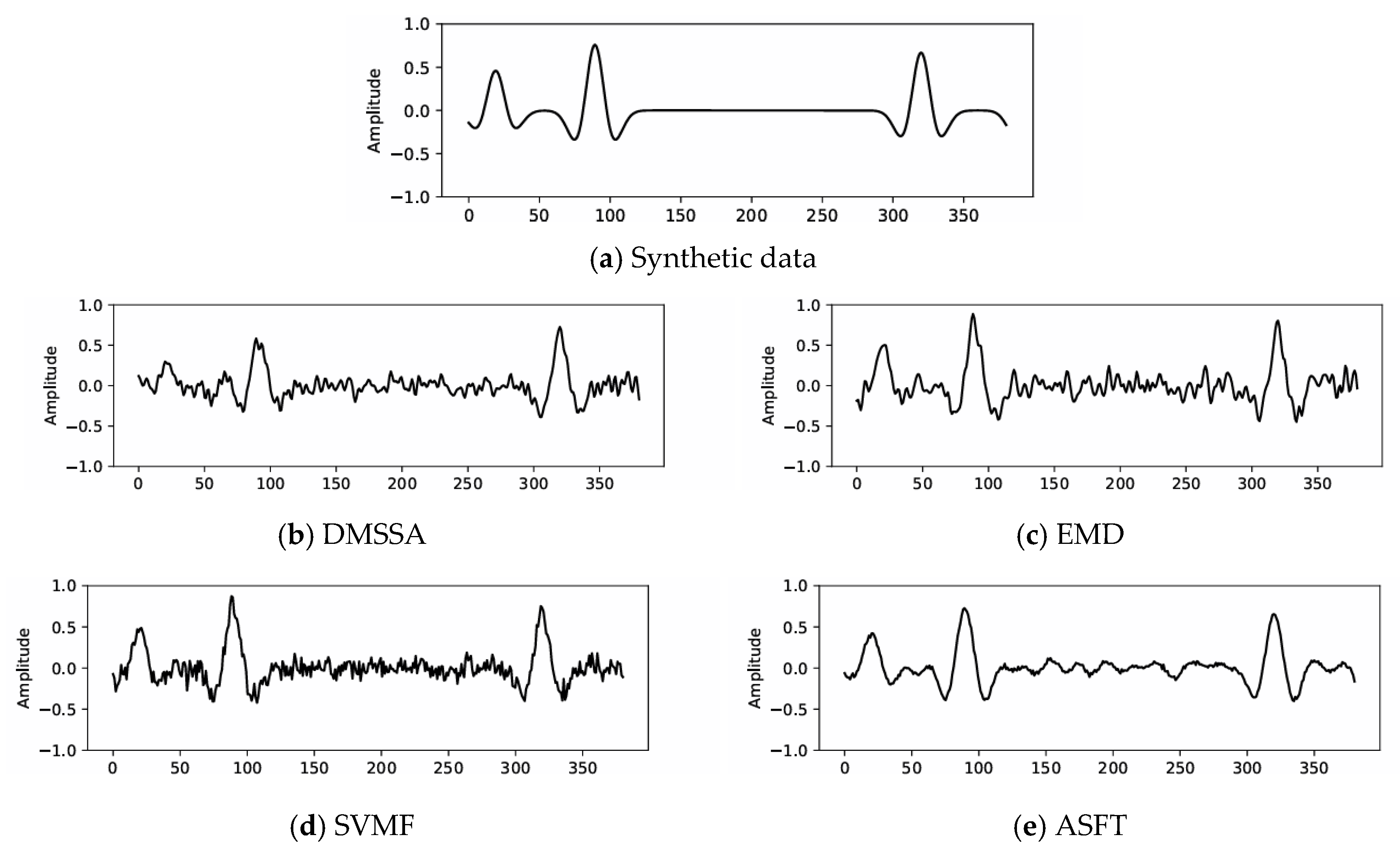
Figure 5.
Synthetic example. (a) is the added Gaussian noise, (b) is the noise suppressed by DMSSA, (c) is the noise suppressed by EMD, (d) is the noise suppressed by SVMF, and(e) is the noise suppressed by ASTF.
Figure 5.
Synthetic example. (a) is the added Gaussian noise, (b) is the noise suppressed by DMSSA, (c) is the noise suppressed by EMD, (d) is the noise suppressed by SVMF, and(e) is the noise suppressed by ASTF.
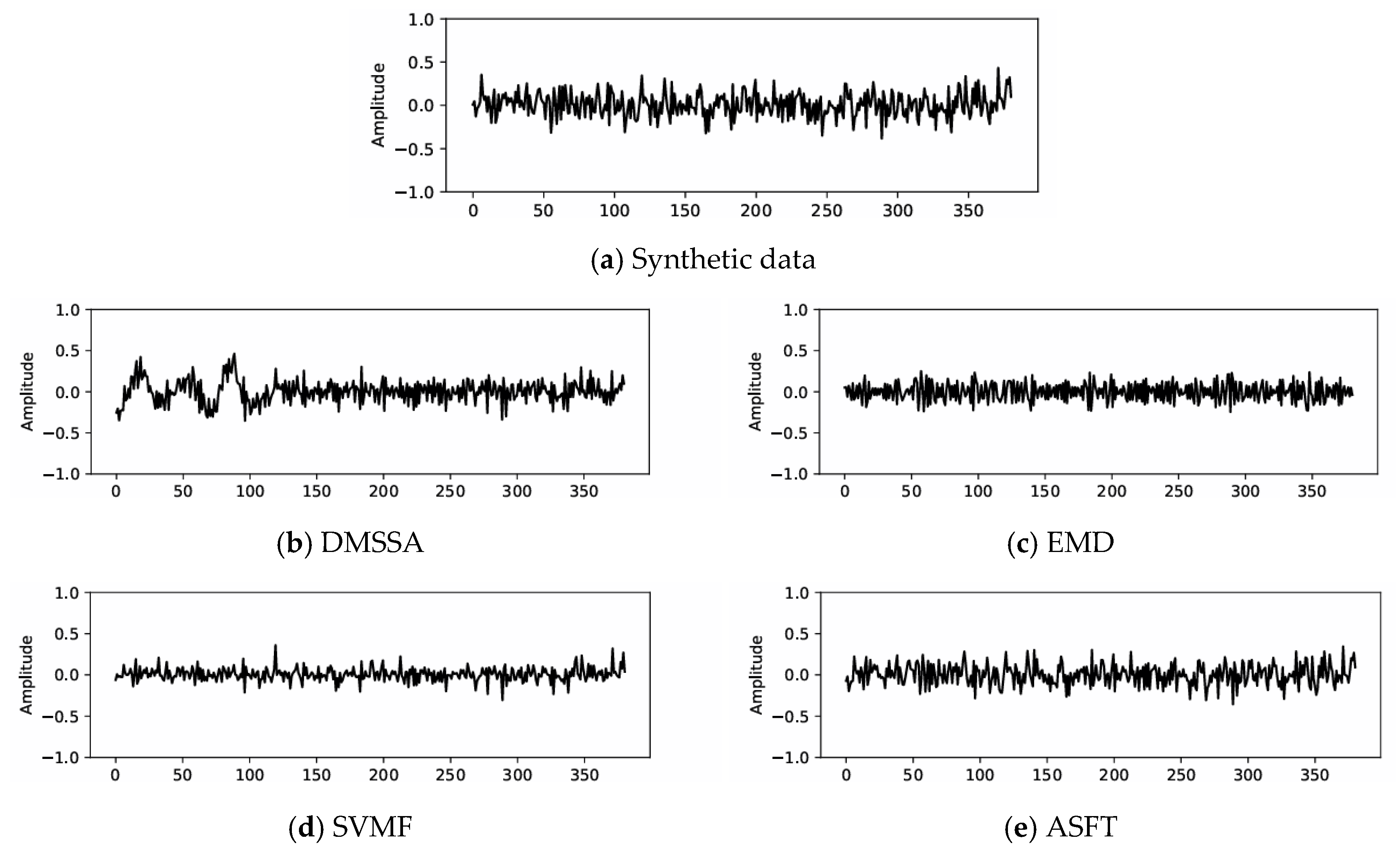
Figure 6.
Synthetic example. (a) is the denoised data in time domain and (b) is the denoised data in frequency domain.
Figure 6.
Synthetic example. (a) is the denoised data in time domain and (b) is the denoised data in frequency domain.
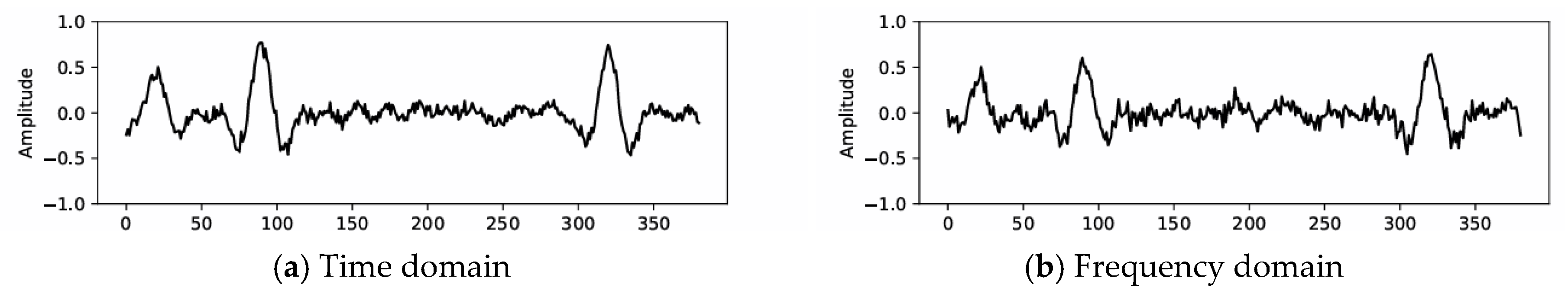
Figure 7.
Synthetic example. (a) is the noise suppressed in time domain and (b) is the noise suppressed in frequency domain.
Figure 7.
Synthetic example. (a) is the noise suppressed in time domain and (b) is the noise suppressed in frequency domain.
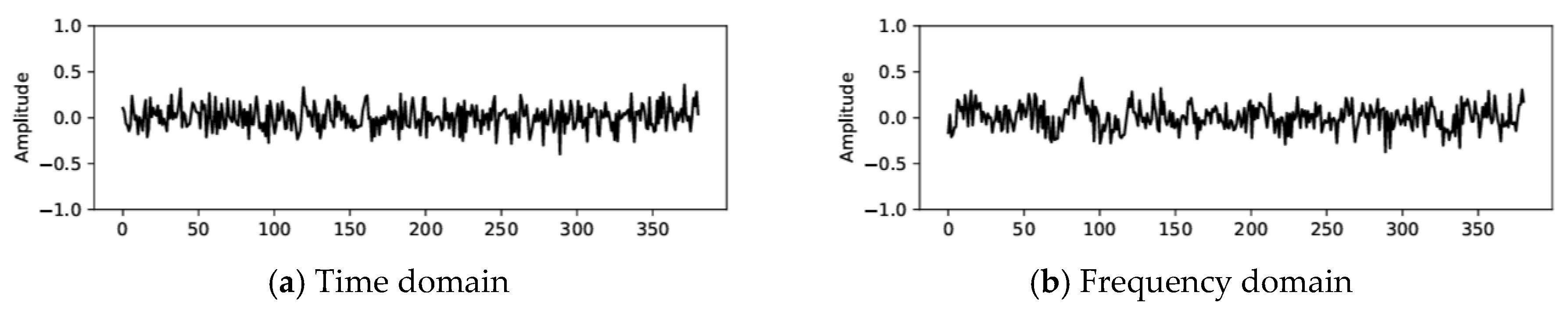
Figure 8.
Shot 1 from field dataset and our denoised result. (a) is field data and (b) is denoised result of ASTF.
Figure 8.
Shot 1 from field dataset and our denoised result. (a) is field data and (b) is denoised result of ASTF.
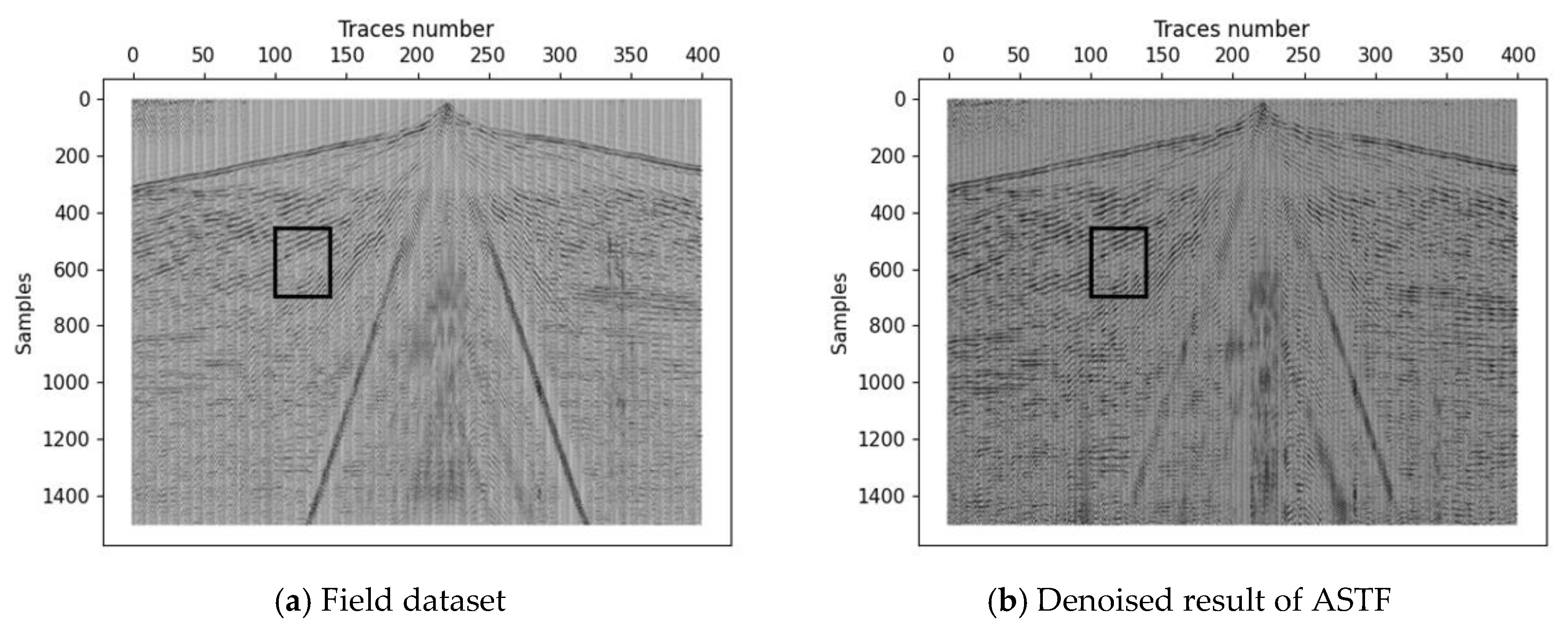
Figure 9.
Denoising effect of part of field data. (a) is part of the field data, (b) is the denoised result of DMSSA, (c) is the denoised result of EMD, (d) is the denoised result of SVMF, and (e) is the denoised result of ASTF.
Figure 9.
Denoising effect of part of field data. (a) is part of the field data, (b) is the denoised result of DMSSA, (c) is the denoised result of EMD, (d) is the denoised result of SVMF, and (e) is the denoised result of ASTF.
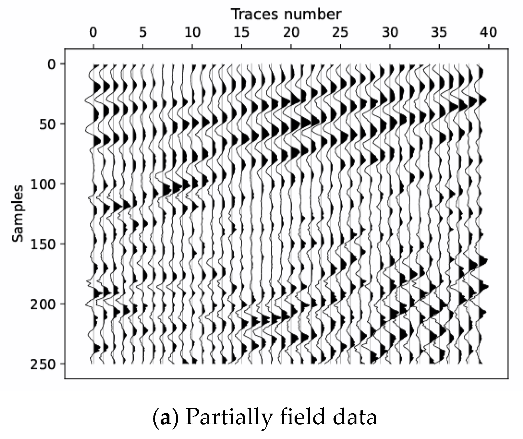
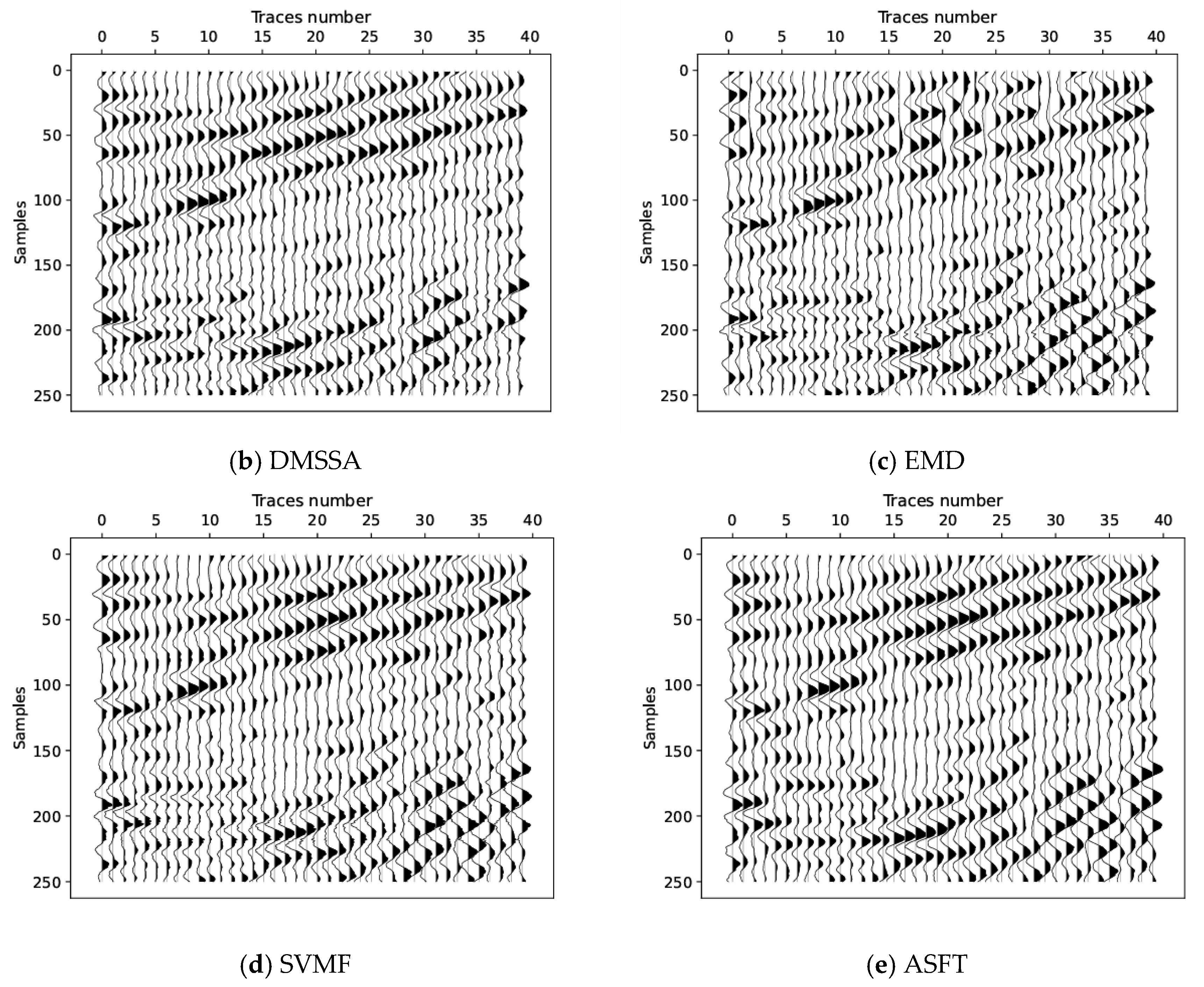
Figure 10.
(a) is the noise suppressed by DMSSA, (b) is the noise suppressed by EMD, (c) is the noise suppressed by SVMF, and (d) is the noise suppressed by ASTF.
Figure 10.
(a) is the noise suppressed by DMSSA, (b) is the noise suppressed by EMD, (c) is the noise suppressed by SVMF, and (d) is the noise suppressed by ASTF.
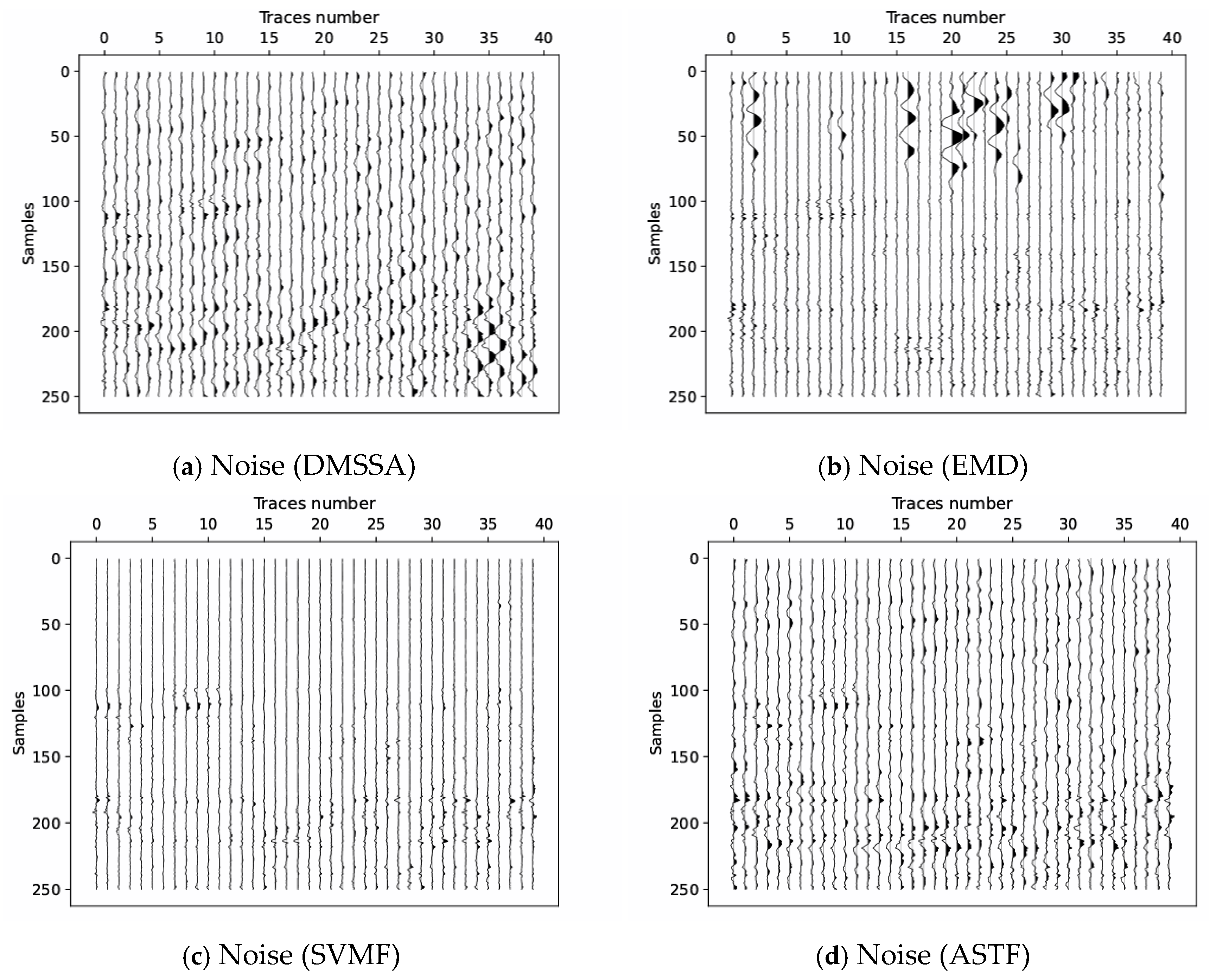

Table 1.
Information of datasets.
| Dataset | Shots | Traces | Samples | Sampling interval | Sources |
|---|---|---|---|---|---|
| dataset1 | 1 | 200 | 1501 | 2ms | Synthetic |
| dataset2 | 1 | 200 | 1501 | 2ms | Synthetic |
| dataset3 | 1 | 200 | 1501 | 2ms | Synthetic |
| dataset4 | 1 | 200 | 1501 | 2ms | Synthetic |
| field dataset | 500 | 400 | 1501 | 4ms | XinJiang |
Table 2.
Comparison of denoising results of different methods on noisy datasets.
| Dataset | Dataset1 | Dataset2 | Dataset3 | Dataset4 | |
|---|---|---|---|---|---|
| Method | SNR(dB) | PSNR(dB) | PSNR(dB) | PSNR(dB) | PSNR(dB) |
| 1 | 16.10 | 11.67 | 14.56 | 16.94 | |
| DMSSA | 3 | 18.78 | 12.76 | 16.62 | 20.80 |
| 5 | 19.87 | 13.18 | 17.35 | 22.65 | |
| 1 | 15.87 | 11.67 | 14.02 | 15.45 | |
| EMD | 3 | 19.50 | 12.77 | 16.20 | 19.41 |
| 5 | 21.29 | 13.11 | 17.27 | 21.58 | |
| 1 | 16.84 | 11.73 | 14.74 | 16.94 | |
| SMF | 3 | 20.77 | 12.71 | 16.80 | 21.25 |
| 5 | 22.66 | 13.09 | 17.53 | 23.11 | |
| 1 | 18.96 | 12.62 | 16.43 | 20.46 | |
| ASTF | 3 | 22.57 | 13.44 | 18.08 | 25.14 |
| 5 | 23.93 | 13.86 | 18.74 | 27.06 | |
Disclaimer/Publisher’s Note: The statements, opinions and data contained in all publications are solely those of the individual author(s) and contributor(s) and not of MDPI and/or the editor(s). MDPI and/or the editor(s) disclaim responsibility for any injury to people or property resulting from any ideas, methods, instructions or products referred to in the content. |
© 2025 by the authors. Licensee MDPI, Basel, Switzerland. This article is an open access article distributed under the terms and conditions of the Creative Commons Attribution (CC BY) license (http://creativecommons.org/licenses/by/4.0/).
Copyright: This open access article is published under a Creative Commons CC BY 4.0 license, which permit the free download, distribution, and reuse, provided that the author and preprint are cited in any reuse.


