
Submitted:
16 September 2025
Posted:
17 September 2025
You are already at the latest version
Abstract
Effective water resource management and risk mitigation in urban environments require an accurate understanding of river flow dynamics. Traditionally, river discharge estimation relies on the rating curve method, which, despite being simple and low-cost, presents significant limitations in complex channels or under transient flow regimes. Aiming for greater accuracy in discharge estimates, this study employed a one-dimensional hydraulic model based on the Standard Step Method for gradually varied flows. High-quality in situ data, including detailed bathymetric surveys and water level measurements, were used for model calibration and validation. Discharge uncertainty was quantified through the estimation of hydraulic parameters (S₀ and n), comparing the Bayesian approaches GLUE and DREAM. The final uncertainty ranges in discharge estimates (Relative Error) using the DREAM method varied between 6.75% and 7.34%, while the GLUE method presented ranges between 7.31% and 8.64%. The DREAM method demonstrated superior performance, including faster processing speed. It was also observed that model accuracy tends to improve with decreasing water surface elevation, indicating the need for longer data collection intervals during extreme events.
Keywords:
standard step method
; glue
; dream
1. Introduction
The historic river discharge monitoring data is important information for urban planning, especially to prevent floods, uncontrolled urban occupation in risk areas, water availability for public and industrial purposes, food scarcity, among other issues [1,2]. With population increasing all over the world more than 80 % are affected by urban flood [3], the expectation is to increase due to the climate changes [4].
Due to the impact on urban population, it is important to highlight the necessity of the knowledge over urban watercourses, especially of river discharge as parameter for urban planners’ decisions on the elaboration of strategies towards flood control, water availability maintenance, and planning urban occupation [5].
The determination of flow rates in watercourses can be done either directly or indirectly [6]. Direct methods involve the use of high-resolution equipment such as the Acoustic Doppler Current Profiler (ADCP), Acoustic Doppler Velocimeter (ADV), or flow meters, among others [7,8,9,10]. However, the application of these instruments in the field requires their direct operation in channels, which may present challenges such as difficult access during flood events, high flow velocity, large depths, or widths [10]. These conditions may, in turn, pose risks to the safety and health of operators [8,11,12,13].
Another difficulty in direct data collection relates to the high costs of the equipment and measurement processes, both for acquisition and maintenance [14], as well as for handling these devices, considering the advanced technology incorporated into the equipment and, in many cases, the lack of financial resources [15]. These challenges may, at times, make it impossible to obtain the necessary flow data for studying channel behaviors for management decision makers [13].
An indirect method for obtaining flow data is the Stage-Discharge Method, that is relatively simple to apply and easy to understand and it does not require sophisticated or high-cost equipment, and has a limited amount of flow data needed to establish the Stage-Discharge relationship, therefore economically viable [12,16,17].
However, despite the method’s feasibility and the large number of hydrometric stations based on it, it can present various simplifications that may increase the uncertainty of the obtained data [11,18]. The Stage-Discharge Method does not consider sections where the channel or cross-section of the water body may undergo variations in its geometry, such as section constriction, sudden widening, the presence of deep pools, dams, or other obstacles that may result in a slow and gradual change in the flow behavior [11,19]. Another limitation of Stage-Discharge Method is related to the amount of data needed to establish the relationship between the water surface elevation and the flow. Although one of the advantages of this method is the relatively limited need for data to create the curve, challenges still exist in obtaining measurements for extreme flow events [20]. In these situations, the water surface can reach high levels, exceeding the natural channel, which intensifies turbulence and sediment concentration. Additionally, the presence of debris, such as tree branches and other objects carried by the current, can compromise the accuracy of equipment and increase operational risks [21] or influence on the channel roughness changing the Stage-Discharge relationship [22]. Thus, for determining extreme flow data, the curve extrapolation can be used, however this may lead to a considerable increase in data uncertaint [14].
Given the high costs and risks associated with direct flow measurement methods and considering that the Stage-Discharge Method may not provide good accuracy under certain conditions, the development of computational models for simulating flow in natural channels has emerged as a promising solution for estimating flow rates in water bodies [8,23]. In this context, researchers have been focusing their efforts on two main approaches. The first addresses situations where flow velocity and flow data are available, reducing the need for detailed bathymetry. The second approach focuses on the absence of flow data, especially for extreme events, but relies on well-detailed bathymetry and monitoring water surface elevation at two distinct points of the water body [12].
Given the difficulties in applying direct methods and the limitations and deficiencies in the accuracy of the Stage-Discharge Method as an indirect approach, this work will rely on computational hydraulic modeling as an indirect method for obtaining flow data, specifically focusing on the second approach, working with more detailed bathymetric data and historical water surface elevation at two distinct points and applying the Standard Step Method, considering the steady flow and physical parameters as Manning’s coefficient of roughness and slope calibrated in Reis et al. [13].
2. Materials and Methods
The studied watercourse is the Meia Ponte River, located within the urban area of the municipality of Goiânia, Goiás State, Brazil. The Meia Ponte River is the primary watercourse responsible for draining the metropolitan region of Goiânia, spanning approximately 41.6 km within the urban area [24]. The delimited study reaches 3.5 km is located between the coordinates 16°36’19.42”S, 49°17’28.69”W (upstream) and 16°37’7.89”S, 49°16’47.71”W (downstream), as shown in Figure 1.
The studied river reach is not fed by any tributaries, presents favorable conditions concerning erosion, and includes two engineered structures (bridges). The climate in the region is characterized by two distinct periods, with the flood season occurring from November to February and the dry season from March to October, respectively.
The methodology employed for flow simulation was based on the well-established Standard Step Method (STM), which forms the basis for steady-flow modeling in the computational program HEC-RAS [25]. Its application requires assuming that the flow is steady and gradually varied, and that the slope is sufficiently small to allow for the assumption of hydrostatic pressure distribution [26]. The model can be formulated as per Equation 1 [26,27]:
where VU and VD represent the water surface elevations at the upstream and downstream sections, respectively; SfU and SfD are the energy slopes at the upstream and downstream sections, respectively; S0 is the channel bed slope; ΔX is the distance between the upstream and downstream sections; and g is the acceleration due to gravity. Additionally, VU and VD denote the mean flow velocities at the upstream and downstream sections, respectively.
In Equation 1, the terms dependent on flow velocity (V) can be expressed as a function of the flow discharge (Q) and the cross-sectional area (A), using the fundamental relationship V = Q/A. This substitution is feasible because the cross-sectional area (A) can be determined as a function of the water surface elevation from obtained bathymetric data. Furthermore, the energy slope terms, SfU and SfD, are determined using the Manning equation for steady flow in open channels (Equation 2) [26,27].
where Q is the flow rate of the study reach, n is the Manning’s roughness coefficient, A is the cross-sectional area, and Rh is the hydraulic radius of the section.
Therefore, Equation 1, which describes the water surface profile, is formulated by expressing velocity (V) as Q/A (where Area A is derived from bathymetric data and water surface elevation) and calculating the energy slope (SfD) using Equation 2 (Manning’s equation). This approach enables the determination of the water surface elevation based on the flow discharge (Q) and channel geometry.
Thus, for the application of the model, it is necessary to know the channel bed slope parameter (S0), Manning’s roughness coefficient (n), the length of the study reach (ΔX), the history of water surface elevations for the upstream and downstream points (y), and bathymetric data for determining the cross-sectional area of the upstream and downstream channels (A). In other words, it is necessary to know the boundary conditions of the flow, for the case of subcritical flow downstream and supercritical flow upstream.
The first two parameters (channel slope, S0, and Manning’s roughness coefficient, n) were determined through a calibration process, applying Bayesian statistics to evaluate the obtained values [13,28]. The input data for S0 and n were determined through the calibration and validation process carried for the same study area and presented in Reis et al. [13], where the GLUE and DREAM methods were applied, based on the works of Beven and Binley [29] and Vrugt [30], respectively.
To obtain distance data in the flow direction (X) and water surface elevation (y), Oliveira et al. [12] relied on remote sensing tools and the installation of direct measurement equipment. In this study, to identify these parameters, Pressure Sensor Registers (Linigraph HOBO U20 series) were installed at two distinct points, measuring water surface variation every 10 minutes over a period of 6 months, part of which occurred during the flood period and the other part during the dry period (Figure 2ab). The distance in the flow direction and the water level elevations for determining the energy slope were obtained by collecting geographic coordinates using the Trimble R6 GPS RTK (Figure 2c), and were subsequently plotted on a satellite image in the QGIS geographic information system software.
Watercourse cross-sectional profiles were determined through bathymetric surveys conducted at the upstream and downstream limits, as well as at three intermediate points. High-resolution equipment, specifically an Acoustic Doppler Current Profiler (ADCP), was utilized for these surveys. Based on the points surveyed in the field, the cross-sections were interpolated with a longitudinal spacing of ΔX = 200 meters, using the REC-HAS computational program.
To determine the uncertainty, water surface elevation data collected in the field through topographic surveys using a GPS RTK were analyzed. While ADCP surveys provide depth, the simultaneous GPS RTK data capture the water surface elevation relative to a geodetic datum. With the upstream and downstream elevations thus determined, the model simulations used the downstream elevation values as input and compared the simulated upstream elevations against the observed upstream data. This approach allowed assessing the model’s performance in simulating the water surface profile from downstream to upstream and quantifying the associated simulation uncertainty.
3. Results and Discussion
Simulations employing the Standard Step Method (STM) were conducted using parameter sets calibrated by two different methods: GLUE and DREAM. For the GLUE calibration, ten most representative parameter sets (n1, n2, n3, S0) were utilized (Table 1). The generation of 100,000 hydraulic parameter sets for GLUE took approximately 4.5 hours, from which these ten sets were selected, with the subsequent simulation requiring 15 minutes. The determined Manning coefficients (n1, n2, n3, S0) from the GLUE calibration are consistent with literature values for the actual conditions encountered [31,32,33]. Conversely, for the DREAM calibration, the ten most representative parameter sets (n1, n2, n3, S0) were used (Table 1), as determined in Reis et al. [11]. The DREAM parameter generation was significantly faster, taking approximately 30 minutes for 100 sets, and the simulation required only 4 minutes. Consistent with the GLUE calibration results, the Manning coefficients (n1, n2, n3) obtained through DREAM calibration also remained consistent with the literature [31,32,33].
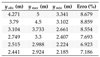
The results obtained with the GLUE method, as illustrated in Table 2, show relative errors in flow simulations for the studied section ranging from 6.923% to 8.859% for observed water surface elevations of 2.515 m and 3.790 m, respectively. A pattern is observed in the relative error results, which tend to decrease as the water surface elevation decreases. This behavior is similar to that observed in the Po River, Italy, where it was concluded that higher flow values generate greater relative errors in their estimations [23].
On the other hand, the results derived from the DREAM method, as illustrated in Figure 3a, show the relative errors in determining water surface elevations using the Standard Step Method model. Here, the largest relative error occurred for an elevation of approximately 693.6 m, reaching 19.63%. Despite this maximum error being close to 20%, most relative errors remained below 8%, with some values even less than 2%. Although the relative errors found in these simulations are considered low, it is important to note that this analysis was performed using only the set of hydraulic parameters with the highest representativeness (Figure 3b). In this specific case, the relative errors were observed to be very close to 0%, except for values near elevations between 693.4 m and 693.7 m, which may indicate some interference during the observed data collection.
The difference in the presentation of results between GLUE and DREAM lies in GLUE’s detailed tabulation of specific errors versus DREAM’s qualitative analysis. This distinction reflects DREAM’s larger data volume, allowing for comprehensive statistical validation. Thus, even without a similar table, DREAM offers a robust view regarding the variation in elevation estimates and accuracy.
The results obtained using the GLUE method, as illustrated in Figure 4a, indicate that the water surface elevations remained within the uncertainty range. This demonstrates the Standard Step Method’s validity for the established parameters and the studied cross-section, as the calculated elevations consistently follow the pattern of observed elevations. Conversely, Figure 4b presents the results from the DREAM method, displaying both maximum and minimum water surface elevations in comparison to observed data. For this analysis, 250 water surface elevations were randomly selected from the upstream cross-section to ensure a broad distribution of values and avoid repetition. It was observed that, while these water levels also remained within the uncertainty range, they were very close to the calculated maximum values. This suggests that the applied model may underestimate the actual elevations.
Furthermore, Figure 4b validates the Standard Step Method model, demonstrating its ability to simulate water surface elevation levels with satisfactory precision. The relative error values obtained from applying this method using GLUE were less than 9%. In contrast, simulations with the DREAM method indicated relative errors close to 20%, which is justified by the use of a significantly larger number of observed elevations as input data. The GLUE method analyzed only 6 different elevations, resulting in a processing time of approximately 15 minutes, while the DREAM method considered around 250 distinct values, requiring only about 4 minutes for processing. Although the GLUE method yielded satisfactory results, the DREAM method proved more efficient and reliable, consuming less time in processing results, as evidenced in studies by Reis et al. [12] and Pereira [28].
Figure 5a shows the comparison between the relative errors obtained from the simulations with parameters determined by the GLUE and DREAM methods. It can be inferred from Figure 4a that, once the outliers are defined, the relative errors for the DREAM method were limited between values of 6.75% and 7.34%, which represents the uncertainty range, and the values were slightly lower compared to those found when the GLUE method was applied, which ranged between 7.31% and 8.64%.
The Manning roughness coefficient values for the parameters calibrated via the GLUE method were around 0.15 for the 10 sets used, while for the DREAM method, they ranged from 0.04 to 0.065. The equivalent roughness coefficient found by the GLUE method would represent channels with high vegetation concentration, deep pools, and flood areas dominated by shrubs, while the values found by the DREAM method would correspond to coefficients found in cases of clean, winding main channels, with some pools and sandbars, but with more rocks and vegetation concentration [31]. According to the field observation, the second option would be more compatible with the site.
Figure 5b illustrates the energy slope values found. The uncertainty range for the application of the DREAM method parameters in the simulations was considerably smaller when compared to the values found by the GLUE method, where the respective uncertainty ranges were from de 0.88 to 7.19 x 10⁻⁴ m/m for the first case and from 3.66 to 18.26 x 10⁻⁴ m/m for the second case. The results presented consistent while comparing the higher values of roughness coefficient found out through GLUE calibration and consequently higher slope values.
The presented results demonstrate that, while both GLUE and DREAM methods provide valid calibrations, the DREAM method stands out by exhibiting lower uncertainties in relative errors and Manning’s roughness coefficients. It also generates roughness coefficients that are more consistent with field observations. The smaller amplitude in energy slope values obtained via DREAM corroborates its higher precision and physical representativeness for the studied system, indicating the superiority of this method for calibrating hydrodynamic models in complex scenarios.
4. Conclusion
This paper analyzed de river flow considering the Standard Step Method based on the Bernoulli’s equation and applied the parameters of roughness and slope estimated in Reis et al. [13] by two different Bayesian statistical method, GLUE and DREAM, forming two groups of varied parameters settings. Based on the results presented, it is possible to observe that the simulations applying the Standard Step Method reached a satisfactory representation when compared to the observed data. The results obtained through the simulations conducted using the Standard Step Method proved as important tool to simulate river discharge while considering steady flow just as observed in Bouabdellah [27], with relative errors found to be below 8.64% for the GLUE method and below 7.34% for the DREAM method (when outliers were discarded).
It is noted that the processing time for both methods was relatively low. However, the DREAM method took less than 1/3 of the time spent, while analyzing approximately 80 times the sample space compared to the GLUE method. Another point to mention is the uncertainty range related to the energy slope, where the DREAM method showed considerably smaller values.
When analyzing the relative errors found in the application of the model, it can be stated that the results were satisfactory. The DREAM method proved to be more effective in calibrating the parameters n1, n2, n3, and S0 compared to the GLUE method. However, it is worth highlighting that the GLUE method also provided good results, and its application would be of lower complexity than the DREAM method [12,28].
Although the results presented were considerably low, during the development of this work and the subsequent analysis of the data, parameters, and results found, it is recommended to collect water surface elevation data with a larger interval (the one used was 10 minutes) and over a longer period (at least one year). It is extremely important to analyze the model’s behavior in simulating flow over a longer period, in order to assess extreme dry and wet periods, since it was observed that the model’s accuracy increased for lower water surface elevations, indicating an increase in relative error during flood periods.
Author Contributions
G.d.C.d.R. wrote the paper and analyzed the data; K. A. S., T.S.R.P. and K.T.M.F. revised the manuscript; G.d.C.d.R. and K.T.M.F. contributed to research development; K.T.M.F. managed the research and development projects. All authors have read and agreed to the published version of the manuscript.
Funding
This study was financed in part by the Coordenação de Aperfeiçoamento de Pessoal de Nível Superior – Brasil (CAPES), grant number 52001016102P4, and financial support by Financiadora de Estudos e Projetos (Finep).
Acknowledgments
The authors thank the support of laboratory of Hydraulics of UFG, and to Tomas Rosa Simões for their technical support in the fieldwork.
Conflicts of Interest
The authors declare no conflict of interest.
References
- GHOSH, P. , SUDARSAN, J. S., & NITHIYANANTHAM, S. (2024). Nature-based disaster risk reduction of floods in Urban Areas. Water Resources Management, 38(6), 1847-1866. [CrossRef]
- SALIMI, M., & AL-GHAMDI, S. G. (2020). Climate change impacts on critical urban infrastructure and urban resiliency strategies for the Middle East. Sustainable Cities and Society, 54, 101948. [CrossRef]
- MICHALIS, E. , GIATRA, C. E., SKORDOS, D., & RAGKOS, A. (2023). Assessing the different economic feasibility scenarios of a hydroponic tomato greenhouse farm: A case study from Western Greece. Sustainability, 15(19), 14233. [CrossRef]
- DHARMARATHNE, G. , WADUGE, A. O., BOGAHAWATHTHA, M., RATHNAYAKE, U., & MEDDAGE, D. P. P. (2024). Adapting cities to the surge: A comprehensive review of climate-induced urban flooding. Results in Engineering, 22, 102123. [CrossRef]
- CEA, L. , & COSTABILE, P. (2022). Flood risk in urban areas: Modelling, management and adaptation to climate change. A review. Hydrology, 9(3), 50. [CrossRef]
- MANFREDA, S. , PIZARRO, A., MORAMARCO, T., CIMORELLI, L., PIANESE, D., & BARBETTA, S. (2020). Potential advantages of flow-area rating curves compared to classic stage-discharge-relations. Journal of Hydrology, 585, 124752. [CrossRef]
- MARDI, M. , & MURMU, S. K. (2024). An Experimental Study of Manning’s Roughness Coefficient with an Acoustic Doppler Current Profiler (ADCP) Method of the River Ganga at Gandhi-Ghat Site, Patna, India. Journal of The Institution of Engineers (India): Series A, 105(4), 987-1001. [CrossRef]
- CHEN, M. , CHEN, H., WU, Z., HUANG, Y., ZHOU, N., & XU, C. Y. (2024). A review on the video-based river discharge measurement technique. Sensors, 24(14), 4655. [CrossRef]
- LOZADA, J. M. D., GARCIA, C. M., OBERG, K., OVER, T. M., & NIETO, F. F. (2023). Improvements to estimate ADCP uncertainty sources for discharge measurements. Flow Measurement and Instrumentation, 90, 102311. [CrossRef]
- DAL SASSO, S.F. , PIZARRO, A., SAMELA, C. et al. Exploring the optimal experimental setup for surface flow velocity measurements using PTV. Environ Monit Assess 190, 460 (2018). [CrossRef]
- CHOO, T.H. , HONG, S.H., YOON, H.C. The estimation of discharge in unsteady flow conditions, showing a characteristic loop form. Environ Earth Science 73 2015, (8): 4451-4460. [CrossRef]
- OLIVEIRA, F. A.; PEREIRA, T. S. R.; SOARES, A. K.; FORMIGA, K. T. M. Uso de modelo hidrodinâmico para determinação da vazão a partir de medições de nível. 2016. Revista Brasileira de Recursos Hídricos, v. 21, n.4, p. 707-718. Porto Alegre, SC. [CrossRef]
- REIS, G. D. C. D. , PEREIRA, T. S. R., FARIA, G. S., & FORMIGA, K. T. M. (2020). Analysis of the Uncertainty in Estimates of Manning’s Roughness Coefficient and Bed Slope Using GLUE and DREAM. Water, 12(11), 3270. [CrossRef]
- ARICÒ, C.; NASELLO, C.; TUCCIARELLI, T. (2009). Using unsteady-state water level data to estimate channel roughness and discharge hydrograph. Advances in Water Resources, 32(8), 1223–1240. [CrossRef]
- PAN, F; WANG, C; XI, X; Constructing river stage-discharge rating curves using remotely sensed river cross-sectional inundation areas and river bathymetry. Journal of Hydrology 540 (2016), 670-687. [CrossRef]
- MUSTE, M. , KIM, D., & KIM, K. (2022). Insights into flood wave propagation in natural streams as captured with acoustic profilers at an index-velocity gaging station. Water, 14(9), 1380. [CrossRef]
- EERDENBRUGH, V; VAN HOEY, K. S.; VERHOEST; N. E. C. (2016), Identification of temporal consistency in rating curve data: Bidirectional Reach (BReach), Water Resour. Res., 52, 6277–6296. [CrossRef]
- MCMILLAN, H. K.; WESTERBERG, I. K. ; Rating curve estimation under epistemic uncertainty. Hydrological Processes 29, 1873-1882 (2015). [CrossRef]
- HAMILTON, S. , WATSON, M., & PIKE, R. (2019). The role of the hydrographer in rating curve development. Confluence: Journal of Watershed Science and Management, 3(1). [CrossRef]
- PAOLETTI, M.; PELLEGRINI, M.; BELLI, A.; PIERLEONI, P.; SINI, F.; PEZZOTTA, N.; PALMA, L. Discharge Monitoring in Open-Channels: An Operational Rating Curve Management Tool. Sensors 2023, 23, 2035. [Google Scholar] [CrossRef] [PubMed]
- CORATO, G.; AMMARI, A.; MORAMARCO, T. ; Conventional point-velocity records and surface velocity observations for estimating high flow discharge. Entropy 2014, 16, 5546–5559. [Google Scholar] [CrossRef]
- D’IPPOLITO, A.; CALOMINO, F.; ALFONSI, G.; LAURIA, A. Flow Resistance in Open Channel Due to Vegetation at Reach Scale: A Review. Water 2021, 13, 116. [Google Scholar] [CrossRef]
- DI BALDASSARRE, G.; MONTANARI, A. (2009). Uncertainty in river discharge observations: a quantitative analysis. Hydrol. Earth Syst. Sci, 13, 913–921. [CrossRef]
- SIEG. Sistema de Informações Geográficas do Estado de Goiás. Secretaria de Estado de Gestão e Planejamento – SEGPLAN 2017. http://www.sieg.go.gov.br/siegdownloads/ (2019).
- CHAUDHRY, M. H. (2008). Open-channel flow. Boston, MA: Springer US. [CrossRef]
- AKAN, A. Osman; IYER, Seshadri S. Open channel hydraulics. Butterworth-Heinemann, 2021.
- BOUABDELLAH, G. (2022). Estimation of River Discharge Outside the Regime of Uniform Flow. Periodica Polytechnica Mechanical Engineering, 66(3), 197-206. [CrossRef]
- PEREIRA, T. S. R. (2015). Modelagem e monitoramento hidrológico das bacias hidrográficas dos córregos Botafogo e Cascavel, Goiânia–GO.
- BEVEN, K.J.; BINLEY, A.M. (1992). The future of distributed models: model calibration and uncertainty prediction. Hydrological Processes, 6(3), 279-298. [CrossRef]
- VRUGT, J.A. “Markov Monte Carlo Simulation using the DREAM software package: Theory, concepts, and MATLAB implementation”. Environmental Modelling & Software 2016. 75, pp. 273-316. [CrossRef]
- CHOW, V.T. Open Channel Hydraulics. New York: McGraw-Hill, 1959, 680p.
- BARNES, H. H., Jr. , (1987) Roughness characteristics of natural channels: U.S. Geological Survey Water-Supply Paper 1849, 213 p.
- ARCEMENT, G. J. Jr; SCHNEIDER, V. R. (1989). Guide for selecting Manning’s Roughness Coefficients for Natural Channels and Flood Plains: U.S. Geological Survey Water-Supply Paper 2339, 38 p.
Figure 1.
Location of the study area.
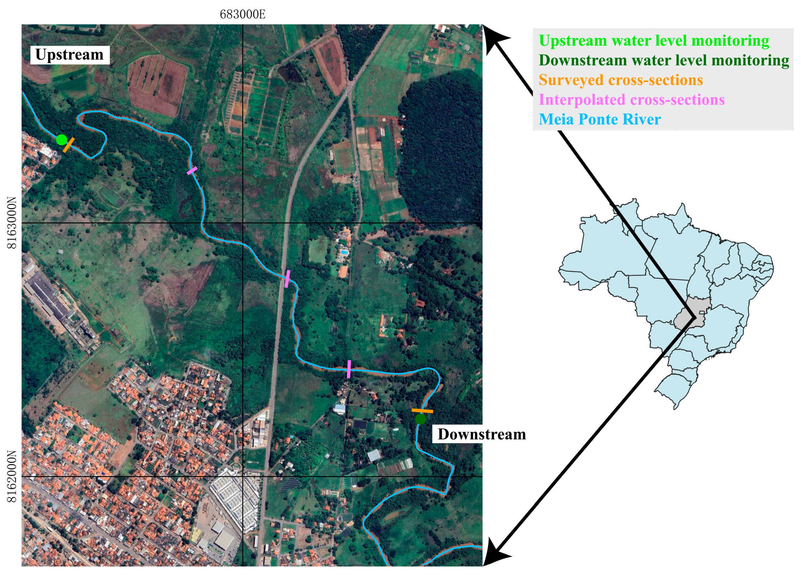
Figure 2.
Obtaining distances in the direction of river flow: a) Pressure Sensor Registers; b) Pressure Sensor Registers installed on the bank of the Meia Ponte river; and c) Collection of geographic location data and water surface elevation.
Figure 2.
Obtaining distances in the direction of river flow: a) Pressure Sensor Registers; b) Pressure Sensor Registers installed on the bank of the Meia Ponte river; and c) Collection of geographic location data and water surface elevation.
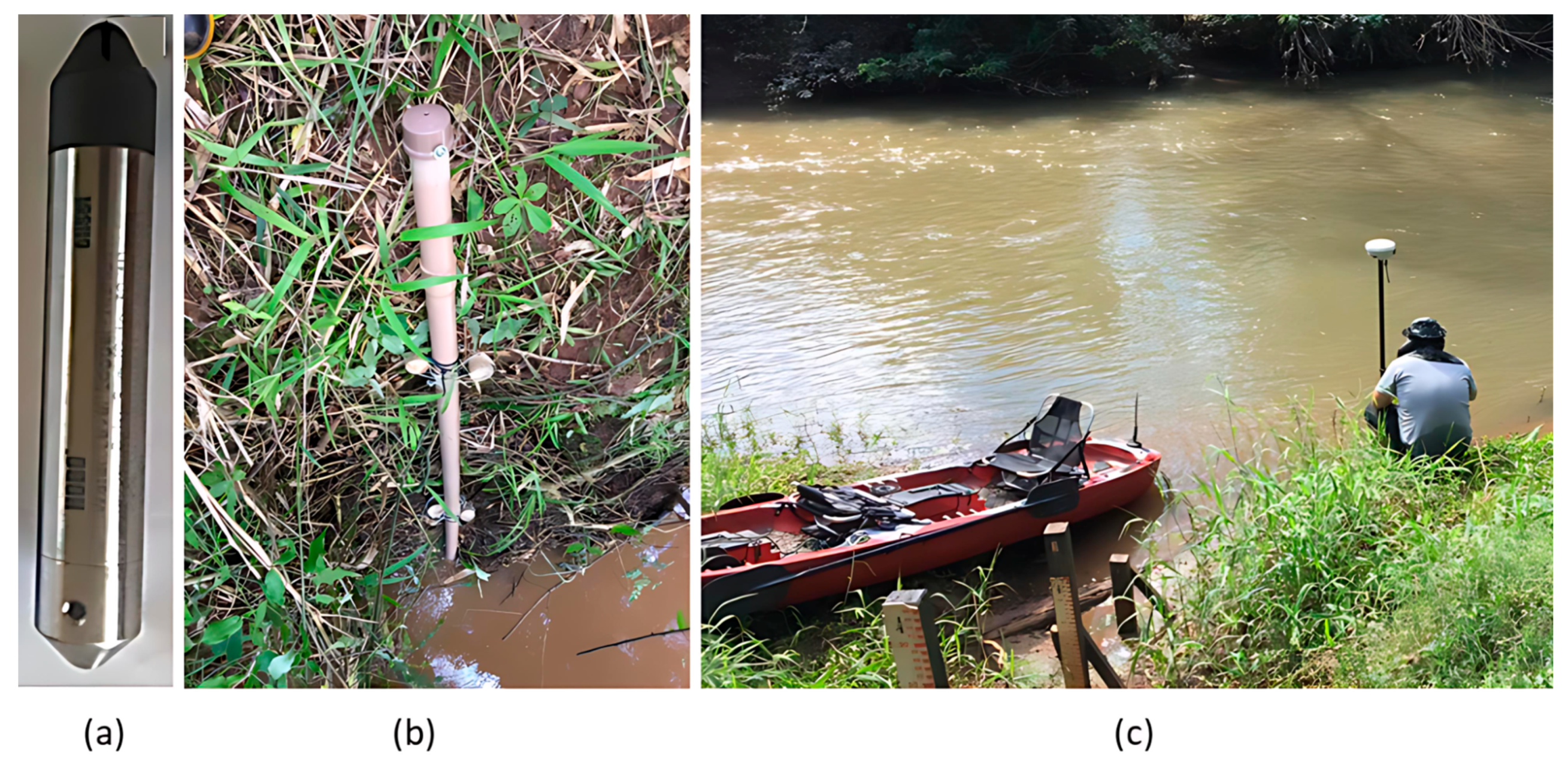
Figure 3.
Distribution of relative errors, applied to the 10 sets of parameters with the greatest representativeness – DREAM method.
Figure 3.
Distribution of relative errors, applied to the 10 sets of parameters with the greatest representativeness – DREAM method.
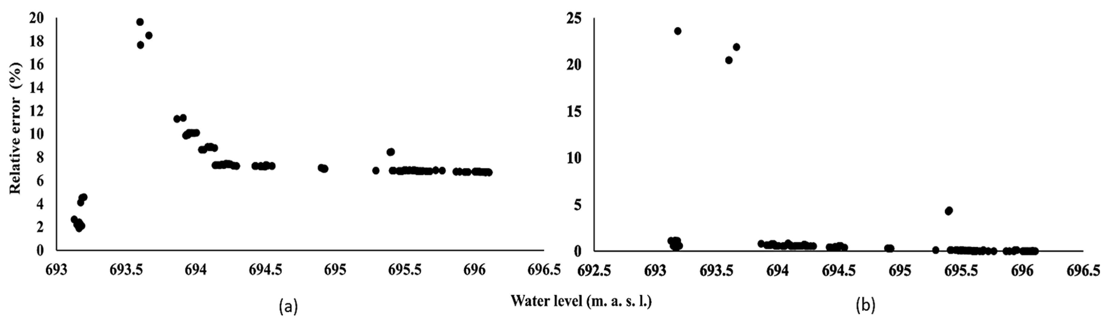
Figure 4.
Distribution of calculated and observed water surface elevations relative to upstream elevation – a) GLUE method and b) DREAM method.
Figure 4.
Distribution of calculated and observed water surface elevations relative to upstream elevation – a) GLUE method and b) DREAM method.
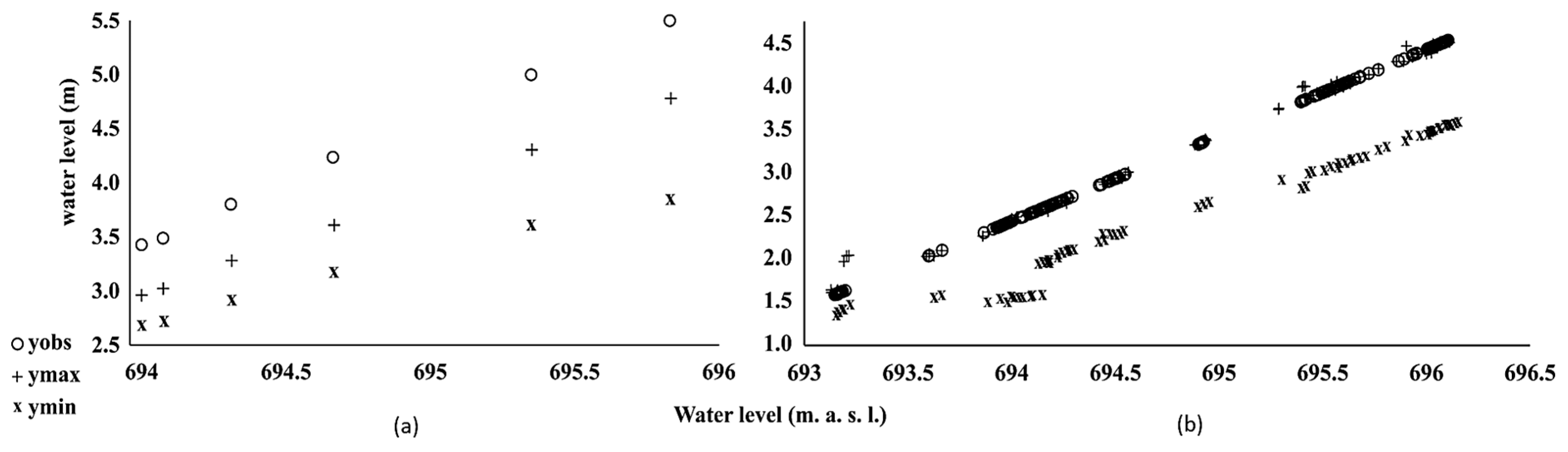
Figure 5.
DREAM and GLUE methods – (a) Relative errors between the simulations performed and (b) Sf calculated intervals.
Figure 5.
DREAM and GLUE methods – (a) Relative errors between the simulations performed and (b) Sf calculated intervals.
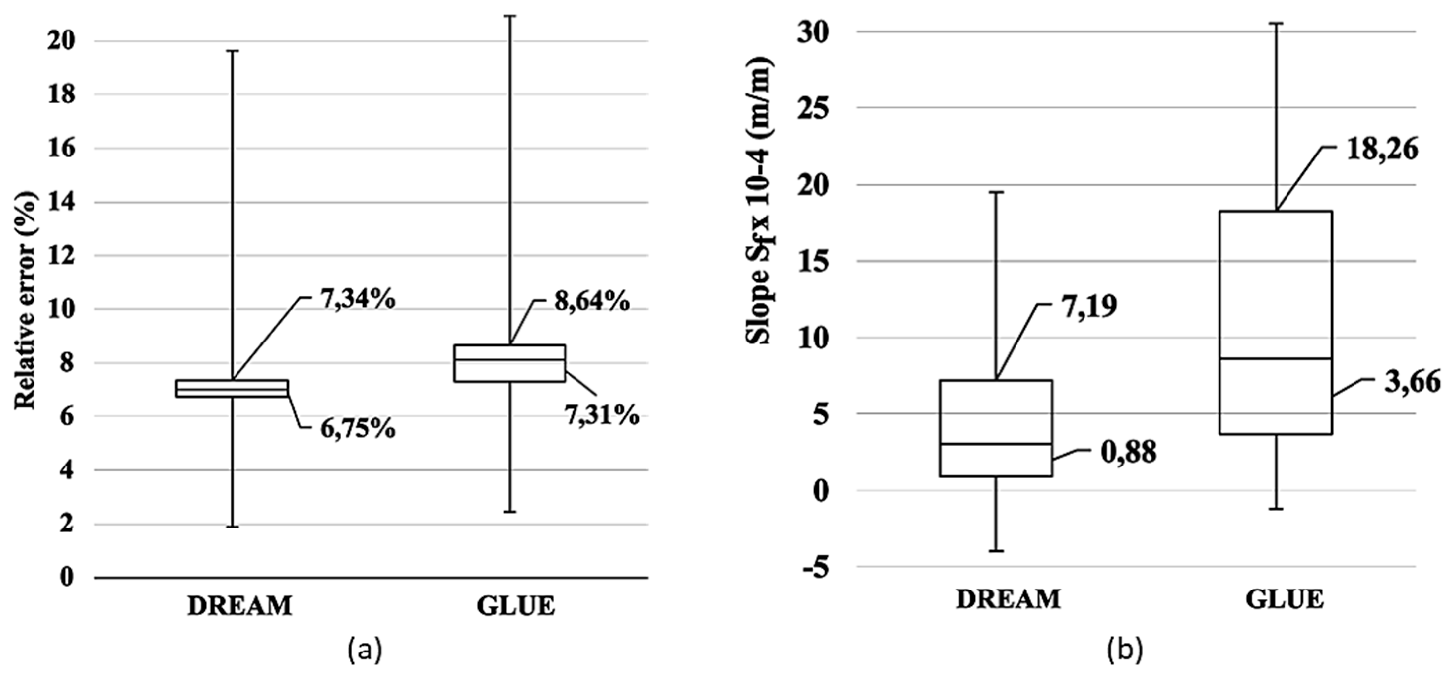

Table 1.
Parameters used as input data in the simulations.
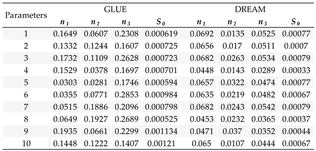
Table 2.
Calculated water surface elevations and associated errors obtained using the GLUE method.
Disclaimer/Publisher’s Note: The statements, opinions and data contained in all publications are solely those of the individual author(s) and contributor(s) and not of MDPI and/or the editor(s). MDPI and/or the editor(s) disclaim responsibility for any injury to people or property resulting from any ideas, methods, instructions or products referred to in the content. |
© 2025 by the authors. Licensee MDPI, Basel, Switzerland. This article is an open access article distributed under the terms and conditions of the Creative Commons Attribution (CC BY) license (http://creativecommons.org/licenses/by/4.0/).
Copyright: This open access article is published under a Creative Commons CC BY 4.0 license, which permit the free download, distribution, and reuse, provided that the author and preprint are cited in any reuse.


