Submitted:
11 September 2025
Posted:
15 September 2025
You are already at the latest version
Abstract
In the domain of mining and mineral processing, depth sensors, including LIDAR and 3D cameras, are employed to obtain precise three-dimensional measurements of the surrounding environment. However, the functionality of these sensors is hindered by the dust produced by mining operations. In order to address this problem, a neural network-based method is proposed. This method is capable of filtering dust measurements in real time from point clouds obtained using LIDARs. The proposed method is trained and validated using both real and simulated data, yielding results that are at the forefront of the field. Furthermore, a public database is constructed using LIDAR sensor data from diverse simulated and real dusty environments. The database will be made public for use in the training and benchmarking of dust filtering methods.
Keywords:
dust filtering
; LIDAR de-noising
; deep learning
; PointNet
1. Introduction
Depth sensors, such as LIDAR (LIght Detection And Ranging) and 3D cameras, are used in mining and mineral processing to provide detailed three-dimensional measurements of the environment. These measurements are used for topographic mapping, rock characterization, autonomous mining vehicle navigation, and obstacle detection, among other applications.
However, mining operations such as blasting, crushing, secondary reduction, and material transport by earthmoving machines and trucks generate dust that can remain suspended in the air for extended periods. Dust particles scatter and absorb light, which introduces noise into depth sensor measurements [1]. This phenomenon can generate false measurements, producing erroneous distance readings, false detections, or missed detections of objects of interest [2]. To address this problem, dust measurements must be filtered from depth sensor readings [3].
Using advanced filtering algorithms can help identify dust signals and separate them from other environmental data. Among other techniques, filtering based on the use of machine learning techniques stands out because statistical classifiers can learn to identify patterns in data [4]. Statistical classifiers can be trained using different types of sensors and information sources, allowing them to adapt to various operating conditions in mining environments. They can significantly improve the accuracy of the 3D data obtained by effectively identifying and differentiating dust measurements.
Two challenges for the use of statistical classifiers in dust filtering are the processing speed and the availability of data for the training of models [3]. Real-time dust filtering is crucial in some applications, such as autonomous navigation and obstacle detection, which require real-time decision making. Regarding the availability of training data, a related requirement is the availability of open dust databases to develop and benchmark different dust filtering methods.
In this paper, we address both challenges. First, we propose a neural network based method capable of filtering dust measurements in real time from point clouds obtained using LIDARs. We train and validate the proposed method using real and simulated data. Second, we build a database using LIDAR sensor data from different simulated and real dusty environments. This database will be made public for use in the training and benchmarking of dust filtering methods.
The main contributions of this paper are: (1) a neural based method for the real-time dust filtering of point clouds obtained with depth sensors, which includes a novel neural network encoding and processing architecture and the use of novel features; and (2) UCHILE-Dust, a database for training and testing dust filtering methods, which will be made public.
2. Related Work
2.1. Traditional Dust Filtering Methods
Traditional dust filtering methods process each element of the point cloud iteratively and filter them considering the local density, the intensity of the measurement, or both.
Statistical Outlier Removal (SOR). Dust filtering is implemented by modeling dust measurement as outliers. For each point of the point cloud, the average distance to a neighborhood of K points is calculated and then compared to a threshold value T given by [3]:
where and are the mean and standard deviation of , respectively, and is a constant to be defined. If the average distance exceeds T, the point is considered an outlier and is filtered.
Radius Outlier Removal (ROR). In this method, the number of points within a sphere with a radius of R centered on each point is calculated [3]. If is smaller than a threshold value N, the point under analysis is considered an outlier. R and N are hyperparameters to be determined.
Dynamic Radius Outlier Removal (DROR) The ROR method tends to fail with LIDAR sensors because the use of a fixed radius cannot handle the variable resolution of the point cloud. In order to address this, DROR [6] proposes using a dynamic radius, , which depends on the distance of the point and the angular resolution of the sensor. For points that are closer to the source, a fixed radious is used; otherwise, the radius is calculated as follows:
where is a constant, is the angular resolution of the LiDAR sensor, and are the Cartesian coordinates of the point under analysis.
Low-Intensity Outlier Removal (LIOR). This method takes into account the fact that the measurements corresponding to the dust have a low intensity [5]. Based on this idea, the LIOR method [7] applies ROR filtering to points whose intensity is lower than a threshold . Points whose intensity is greater than are not filtered.
Low-Intensity Dynamic Radius Outlier Removal (LIDROR). The method proposed in [8] improves LIOR by implementing DROR filtering instead of ROR filtering, which means that a variable radius is used for filtering.
According to [3], LIDROR performs better than the SOR, ROR, DROR, and LIOR methods when it comes to dust filtration.
2.2. Machine Learning Based Dust Filtering Methods
The basic idea of these methods is to use a statistical classifier to determine if a point (measurement), or the points contained in a voxel, correspond to dust or not. Methods that use features computed on the voxels calculated from the point cloud are called voxel-wise methods, while methods that use the points of the point cloud directly are called point-wise methods. Naturally, point-wise methods are preferred because they are able to filter individual dust measurements.
Any statistical classifier can be used to perform the point-wise/voxel-wise classification, although only the use of Support Vector Machines (SVM), Random Forests (RF) and Neural Networks (NN) has been reported in dust-filtering [2,3,4,9]. Regarding the employed features, the voxel-wise methods use the mean intensity and standard deviation of the points inside each voxel, as well as appearance features that characterize the type of material that reflect the sensors’ measurements. Some of the most commonly used appearance features are roughness [2,3,4], slope [2,3], planarity [3,4], and curvature [3,4]. These features are calculated from the eigenvalues obtained after performing a PCA projection of the voxel points.
In [2], voxel-wise classification was implemented using SVM, RF and NN classifiers. As features, mean intensity, standard deviation, roughness, and slope were used. The neural network classifier obtained the best results. In [3] also, voxel-wise classification was implemented using the same classifiers. For SVM and RF classifiers, the mean intensity, standard deviation, slope and roughness were used as features, while for the NN classifier, the mean intensity, standard deviation, planarity, curvature and the third eigenvalue were employed. The best results were obtained by the RF and NN classifiers. In [4], a CNN (Convolutional Neural Network) was used to implement a voxel-wise classification using as features the mean intensity, standard deviation, roughnes, planarity and curvature.
In [9], point-wise classification was implemented using a U-net (an encoder-decoder type of CNN architecture), which required the point cloud to be transformed into a 2D LIDAR image. In this image, each pixel corresponds to a LIDAR measurement, and the rows and columns correspond to the vertical and horizontal angles of the measurement, respectively. Given that a multi-echo LIDAR was used, the inputs to the U-net were the range and intensity values for the first echo and the last echo, in each image position. The authors compare the proposed point-wise architecture with a voxel-wise architecture implemented using a standard CNN. The proposed point-wise architectura obtained slightly better results than the voxel-wise one.
The main drawback of the reported methods based on the use of statistical classifiers is that most of them employ a voxel-wise classification, which does not allow for the filtering of single measurements corresponding to dust; instead, voxels are classified as dust. This makes it hard to use these methods in cases where small details need to be determined (e.g., the characterization of small structures or the detection of small obstacles from a mobile vehicle). In the case of using a point-wise classification [9], the 2D projection of the point cloud lost 3D spatial information.
Therefore, there is a need for point-wise architectures for dust filtering that can fully utilize the 3D information contained in the point cloud. In the following section, we present a neural architecture capable of performing this kind of processing.
3. Proposed Dust Filtering Method
The proposed dust filtering method is based on the use of a modified version of the PointNet++ architecture [11], which receives point cloud data directly, groups the points hierarchically, computes internal feature representations, and classifies each point as dust or non-dust. For each LIDAR measurement, its 3D position, intensity, and temporal displacement are provided to the network. In the case where the data scan is acquired from a mobile vehicle, odometry information is also considered. Thus, the dust-filtering process takes into account geometric, intensity, and temporal features.
3.1. Neural Architecture: Reduced-PointNet++
The PointNet network, proposed in [10], is able to directly process the spatial coordinates and other attributes of the points to classify and segment a point cloud. Unlike previous approaches that required converting the point clouds into 2D or volumetric representations, PointNet works directly on 3D data without the need for voxelization or projections, which makes it more efficient in terms of memory and processing. PointNet is based on the use of symmetric functions, such as global max-pooling, which allows it to be invariant to the order of the points, a fundamental property in point clouds where there is no predefined order. In addition, the model incorporates learned transformations that align the point cloud before processing, reducing the variability introduced by differences in data orientation. However, due to its reliance on global feature aggregation, PointNet is limited in its ability to capture local relationships between points, which may affect its performance on tasks that require fine-structure information, as in the case of filtering dust measurements.
PointNet++, proposed in [11], improves PointNet by using hierarchical groupings of PointNet points and subnetworks on multiple scales, allowing greater capture of local features and spatial relationships. This modification allowed its use for dust filtering.
In order to achieve real-time processing of large point clouds, a reduced version of PointNet++ was designed in this work. Two big changes were made to PointNet++: first, the number of sampled points was reduced, which also reduced the number of abstraction layers (SA), and some blocks were eliminated to make the architecture simpler. Second, the MLPs configurations in both the abstraction and propagation blocks were adjusted. This led to a significant decrease in the number of parameters and an improvement in the efficiency of the model. Table 1 shows these changes.
In Section 4, a comparison of the performance of PointNet++ and its reduced version is presented in dust-filtering tasks.
3.2. Point Cloud Features
Let us consider a point cloud containing points belonging to frame t, where t represents an instant in a temporal sequence of length T. Each point is defined by:
where corresponds to spatial data and represents a vector of associated attributes, such as intensity () or other properties such as temporal information.
A first alternative to incorporate temporal information is to find the spatial differences between points in consecutive point clouds. For each point in , we look for the nearest point in . This is done by minimizing the following Euclidean distance:
Then, the nearest point is determined as:
and the spatial difference vector is computed as:
The vector of spatial differences , or its magnitude , can then be used as a temporal attribute of each point.
A second alternative to incorporate temporal information, proposed in [12] as temporal variation-aware interpolation, is to generate an interpolated feature to represent the local information of the previous point cloud projected in the current point cloud . To do this, first, for each point in , we calculate the distances to the K nearest neighbors in . Then, the interpolation weights for each neighbor point are computed as follows:
with defined by (4) and and hyperparameters.
The weights are then normalized using the softmax function:
Then, for each of the nearest neighbor points of in the previous point cloud, the intensity value and the differences of the intensity values are fed to an MLP layer with ReLU activation, and intermediate features are computed (see details of the network architecture in [12]):
Afterward, all intermediate features are agregated to generate the interpolated feature as:
where ⊙ is an elemental multiplication.
As shown in Table 2, different variants of our dust filtering method can be built depending on the information (feature vector) used:
- SI: Spatial + Intensity features.
- STdm: Spatial + Temporal-magnitude-difference features.
- STdv: Spatial + Temporal-vector-difference features.
- STi: Spatial + Temporal-interpolated features.
- SITdm: Spatial + Intensity + Temporal-magnitude-difference features.
- SITdv: Spatial + Intensity + Temporal-vector-difference features.
- SITi: Spatial + Intensity + Temporal-interpolated features.
Finally, in the case where the 3D data are acquired from a LIDAR mounted in a moving vehicle or robot, the odometry information is used to align the point clouds before the temporal features are computed. Thus, before calculating temporal features between point clouds and , the points of are projected to t using the rotation and translation matrices between and t, and , respectively. These matrices are calculated from the vehicle’s odometry.
4. Experimental Results
4.1. UCHILE-Dust Database
The UCHILE-Dust dataset consists of real-world LIDAR point clouds captured using an OS0 sensor in various indoor and outdoor environments under dusty conditions. Each recording spans 15 seconds to 2 minutes, during which dust is actively dispersed in the scene. Each LIDAR frame is treated as an individual point cloud.
Recordings were saved either as PCAP files (direct OS0 stream) or ROS bag files (robot-mounted OS0 with odometry). A multi-step preprocessing pipeline was applied, including frame extraction, odometry alignment (moving sensor case), multi-echo merging, distance filtering, pre-labeling with dust-free references, manual annotation using labelCloud, and final conversion to the S3DIS (Stanford Large-Scale 3D Indoor Spaces) format. Table 3 shows a general overview of the database, considering the different subsets captured in different environments. It is important to note that the percentage of dust points in all subsets is less than 12%.
Interior 1 & 2 Subsets
Captured indoors at the Field Robotics Laboratory of the Advanced Mining Technology Center (AMTC) of the Universidad de Chile (UCHILE) using a static OS0 LiDAR sensor. Dust was manually dispersed across the scene, which includes a combination of glass and concrete surfaces that introduce complexities with transparent and reflective materials. A rock breaker hammer is present in the center of the room.
Exterior 1 & 2 Subsets
Outdoor captures in the AMTC courtyard. Dust was dispersed either between the sensor and a nearby wall or in open space to assess the impact of multi-path reflections.
Carén Subset
Captured in a large, dry, and windy open field with flat terrain and a quarry. The site is located in the Metropolitan Region of Chile and belongs to the UCHILE. A Panther robot equipped with an OS0 LiDAR was used to collect data while in motion. Dust was introduced using an air blower. Carén is the most realistic subset for mobile perception tasks.
Example point cloud frames for each subset are shown in Figure 1.
4.2. Experimental Setup
Each variant of the model (SI, STdm, STdv, STi, SITdm, SITdv, and SITi) was trained using its respective training and validation sets. Three different learning rates were used for each variant: 0.01, 0.008, and 0.005. The learning rate that produced the best results was selected. This was done because the average accuracy varied depending on the learning rate used in each experiment. In all cases a batch size of 16 was used. Other hyperparameters used are the following:
- The CrossEntropyLoss was used as a loss function but considering weights for the classes, since they are unbalanced. This weight consisted of the inverse of the proportion of each class within the corresponding training dataset.
- The number of training epochs was set at 100, but Early Stopping was implemented with 10 epochs of patience relative to the average accuracy value in the validation set. This metric was chosen as it is invariant to class imbalance.
- Data Augmentation methods were used: rotations, scaling, occlusion, and noise.
- A dropout rate of 0.7 was used to reduce overfitting and was applied to the last convolution layer before the classification layers.
As a baseline, the LIDROR method was used. The LIDROD parameters were determined using grid search and the following ranges: , , , and . Table 4 shows the parameters obtained. The parameter is the angular resolution of the sensor; it depends on the LIDAR model and was set to 0.006134.
The following metrics were employed to assess the quality of the various methods employed for dust classification: accuracy, precision, recall and F1-score. Accuracy is the proportion of all classifications that are correct, precision is the proportion of dust classifications that are actually dust, recall is the proportion of actual dust samples that are correctly classified as dust, and F1-score is the harmonic mean of precision and recall.
4.3. Results in Real Environments with Static Sensors
The results of applying different dust-filtering methods to the Interior 1, Interior 2, Exterior 1, and Exterior 2 datasets are shown in Table 5, Table 6, Table 7 and Table 8, respectively. In each instance, the methods are trained using exclusively data from the corresponding datasets. Table 2 presents the features utilized by the variants of the proposed neural-based method, while Table 4 shows the parameters of the LIDROR baseline method.
The results obtained allow for the following conclusions to be drawn. All variants of the proposed method demonstrate superior performance compared to the baseline, with the exception of SITdv when applied to the Interior 1 dataset. In the Interior 2 and Exterior 1 datasets, at least one of the proposed methods achieves an acceptable precision value (greater than or equal to 0.68).
The most challenging datasets are Interior 1 and Exterior 2. In these datasets, all methods have low precision. Given that in deployment in a real environment false positives can be costly, this dataset represents an ideal benchmark for further experimentation. Furthermore, low F1-Scores are expected in these kinds of datasets and are driven by the large imbalance between classes.
Finally, a comparison of the proposed variants reveals that the utilization of both temporal difference and intensity features is generally superior to the application of either temporal differences or intensity features alone.
4.4. Results in Real Environments with Moving Sensors
The results of applying different dust-filtering methods to the Carén dataset, in which the LIDAR sensor is mounted on a mobile robot, are shown in Table 9 and Table 10. Table 9 shows the results when the odometry correction is not used, and Table 10 shows the results when the odometry correction is used.
The results obtained allow for the following conclusions to be drawn. All variants of the proposed method largely outperform the baseline. In fact, LIDROR achieves very low precision with this dataset. Secondly, most of the results obtained by the proposed variants improve when odometry correction is used. The only two cases in which the accuracy decreases are those corresponding to the STi and STdv variants. The best results are obtained by the SITdv variant, with a precision value of 0.7, a recall of 0.97, and an F1-score of 0.82.
4.5. Measuring the Generalization Capabilities of the Method
To measure the generalization of the variants of the proposed methods, all methods were trained and validated using the Interior 1, Interior 2, Exterior 1, and Exterior 2 datasets but tested using the Carén dataset. The results of these experiments are shown in Table 13 and Table 12 for cases with and without odometry.
Upon comparing the results of the methods trained and validated using the Carén dataset (Table 9 and Table 10) reveals that there is only a slight advantage to in-domain training relative to training in one environment and testing in another (Table 13 and Table 12). This finding indicates that the model is learning underlying dust features rather than environment-specific features, such as the relative position of the objects in the scene. This finding suggests that the model is generalizing correctly.
A second conclusion is that, under this experimental setup, the benefits of using odometry correction are lost; in most cases, no improvement in results is observed. One possible reason is that the training and validation sets do not consider the correction of odometry.

Table 11.
Generalization results. Training in AMTC datasets, testing in Carén dataset. No odometry correction
Table 11.
Generalization results. Training in AMTC datasets, testing in Carén dataset. No odometry correction
| Method | Learn. Rate | Accuracy (avg) |
Precision (dust) |
Recall (dust) |
F1-Score (dust) |
| SI | 0.005 | 0.98 | 0.58 | 0.98 | 0.73 |
| STdm | 0.008 | 0.96 | 0.46 | 0.95 | 0.62 |
| STdv | 0.005 | 0.95 | 0.41 | 0.95 | 0.57 |
| STi | 0.005 | 0.96 | 0.64 | 0.94 | 0.76 |
| SITdm | 0.005 | 0.98 | 0.60 | 0.98 | 0.74 |
| SITdv | 0.008 | 0.97 | 0.54 | 0.98 | 0.70 |
| SITi | 0.01 | 0.98 | 0.57 | 0.98 | 0.72 |
Table 12.
Generalization results. Training in AMTC datasets, testing in Carén dataset, with odometry correction
Table 12.
Generalization results. Training in AMTC datasets, testing in Carén dataset, with odometry correction
| Method | Learn. Rate | Accuracy (avg) |
Precision (dust) |
Recall (dust) |
F1-Score (dust) |
| SI | 0.008 | 0.98 | 0.56 | 0.98 | 0.71 |
| STdm | 0.008 | 0.96 | 0.50 | 0.96 | 0.66 |
| STdv | 0.005 | 0.96 | 0.49 | 0.95 | 0.65 |
| STi | 0.01 | 0.96 | 0.52 | 0.95 | 0.67 |
| SITdm | 0.005 | 0.98 | 0.60 | 0.98 | 0.75 |
| SITdv | 0.008 | 0.98 | 0.58 | 0.98 | 0.73 |
| SITi | 0.008 | 0.98 | 0.57 | 0.98 | 0.72 |
4.6. Performance Comparison between PointNet++ and reduced-PointNet++
As a final experiment, a comparison was carried out between using the original PointNet++ architecture and the reduced PointNet++ architecture proposed here, for all of the methods presented in this work.
All experiments were carried out on a platform with a 12 GB VRAM NVIDIA GTX TITAN GPU, a 12-core Intel® Core™ i7-8700K processor running at 3.70 GHz, and 16 GB of RAM. Table 13 shows a comparison of the execution times of both architectures. It can be seen that the reduced PointNet++ architecture outperforms the original PointNet++ architecture in terms of speed. The execution times are, on average, 50% shorter.
It must be noted that this reduction in execution time does not sacrifice performance. Table 14 shows the results of using the original PointNet++ architecture when the methods are trained on the Interior 1, Interior 2, Exterior 1, and Exterior 2 datasets but tested on the Carén dataset, without using odometry information. These results are directly comparable to those in Table 13. Comparing both tables reveals that the results are similar. In some cases, the original PointNet++ obtains slightly better results, while in others, the proposed reduced PointNet++ obtains slightly better results.
These results show that reducing the network size is a valid approach for the dust detection problem, but it also shows that there is still room for further prunning since the reduction in parameters did not affect performance.
Table 13.
Comparison of the execution times of PointNet++ versus reduced-PointNet++.
| Method | PointNet++ (s) | reduced-PointNet++ (s) |
| SI | 0.1383 | 0.0676 |
| STdm | 0.1398 | 0.0672 |
| STdv | 0.1419 | 0.0679 |
| STI | 0.1420 | 0.0694 |
| SITdm | 0.1372 | 0.0710 |
| SITdv | 0.1435 | 0.0664 |
| SITi | 0.1435 | 0.0630 |
| Average | 0.1409 | 0.0675 |
Table 14.
Generalization results obtained using the original PointNet++ architecture. Training in AMTC datasets, testing in Carén dataset. No odometry correction.
Table 14.
Generalization results obtained using the original PointNet++ architecture. Training in AMTC datasets, testing in Carén dataset. No odometry correction.
| Method | Learn. Rate | Accuracy (avg) |
Precision (dust) |
Recall (dust) |
F1-Score (dust) |
| SI | 0.005 | 0.98 | 0.55 | 0.98 | 0.71 |
| STdm | 0.005 | 0.96 | 0.46 | 0.96 | 0.62 |
| STdv | 0.005 | 0.95 | 0.51 | 0.94 | 0.66 |
| STi | 0.01 | 0.96 | 0.51 | 0.96 | 0.67 |
| SITdm | 0.005 | 0.98 | 0.58 | 0.98 | 0.73 |
| SITdv | 0.005 | 0.98 | 0.62 | 0.97 | 0.76 |
| SITi | 0.008 | 0.98 | 0.61 | 0.97 | 0.75 |
5. Discussion
This work presents a real-time dust filtering method for LIDAR point clouds based on a reduced PointNet++ architecture. From the results obtained, it is clear that the proposed approach outperforms the baseline heuristic method. Furthermore, the experiments demonstrated that temporal information is useful in distinguishing dust from static objects, and the integration of odometry further improved the performance in mobile applications.
This is a promising approach for robotic applications in challenging dust-filled environments, since it allows to filter dust from LiDAR measurements in order to perform basic navigation tasks such as SLAM, object avoidance, and emergency stops. Furthermore, the proposed reduction of the network size, which in turn reduces the computational requirements and inference times, allows the network to be deployed in embedded systems such as those found in robotic platforms, which are usually constrained by restrictions such as size and, for dusty environments, passive cooling.
The appoach was tested and developed using the UCHILE-Dust dataset, which will be made publicly available to support the development and benchmarking of future methods. The dataset includes indoor, outdoor, and mobile robot recordings, covering a wide range of scenarios with varying dust densities, allowing for a wide range of possible applications. Our experiments showed that models trained on UCHILE-Dust generalized well from static environments to mobile robot deployments. This suggests that models trained on this dataset learn dust-specific features rather than environment-specific features such as the relative positions of the objects in the scene (layout).
Author Contributions
Conceptualization, B.C., N.C. and J.R.; methodology, B.C. and N.C; software, B.C. and N.C; validation, B.C., N.C. and J.R.; formal analysis, B.C., N.C. and J.R.; investigation, B.C., N.C. and J.R.; resources, J.R.; data curation, B.C., N.C.; writing—original draft preparation, B.C., N.C. and J.R.; writing—review and editing, B.C., N.C. and J.R.; visualization, B.C. and N.C; supervision, N.C. and J.R.; project administration, J.R.; funding acquisition, J.R. All authors have read and agreed to the published version of the manuscript.
Funding
This research was funded by the National Research and Development Agency (ANID) of Chile through project grant AFB230001 for the Advanced Mining Technology Center (AMTC).
Conflicts of Interest
The authors declare no conflicts of interest.
References
- Heinzler, R., Piewak, F., Schindler, P., y Stork, W., “Cnn-based lidar point cloud de- noising in adverse weather”, IEEE Robotics and Automation Letters, vol. 5, p. 2514– 2521, apr 2020. [CrossRef]
- Stanislas, L., Suenderhauf, N., y Peynot, T., “Lidar-based detection of airborne particles for robust robot perception”, en Proceedings of the Australasian Conference on Robotics and Automation (ACRA) 2018 (Woodhead, I., ed.), Australasian Conference on Robo- tics and Automation, ACRA, pp. 1–8, Australia: Australian Robotics and Automation Association (ARAA), 2018, https://eprints.qut.edu.au/125130/.
- Afzalaghaeinaeini, A., Design of Dust-Filtering Algorithms for LiDAR Sensors in Off- Road Vehicles Using the AI and Non-AI Methods. Tesis PhD, University of Ontario Institute of Technology, 2022.
- Parsons, T., Seo, J., Kim, B., Lee, H., Kim, J.-C., y Cha, M., “Dust de-filtering in lidar applications with conventional and cnn filtering methods”, IEEE Access, vol. PP, pp. 1–1, 01 2024. [CrossRef]
- Phillips, T., Guenther, N., y Mcaree, P., “When the dust settles: The four behaviors of lidar in the presence of fine airborne particulates”, Journal of Field Robotics, vol. 34, 02 2017. [CrossRef]
- Charron, N., Phillips, S., y Waslander, S. L., “De-noising of lidar point clouds corrupted by snowfall”, en 2018 15th Conference on Computer and Robot Vision (CRV), pp. 254–261, 2018. [CrossRef]
- Park, J.-I., Park, J., y Kim, K.-S., “Fast and accurate desnowing algorithm for lidar point clouds”, IEEE Access, vol. 8, pp. 160202–160212, 2020. [CrossRef]
- Afzalaghaeinaeini, A., Seo, J., Lee, D., y Lee, H., “Design of dust-filtering algorithms for lidar sensors using intensity and range information in off-road vehicles”, Sensors, vol. 22, no. 11, 2022. [CrossRef]
- Stanislas, L., Nubert, J., Dugas, D., Nitsch, J., Sünderhauf, N., Siegwart, R., Cadena, C., y Peynot, T., Airborne Particle Classification in LiDAR Point Clouds Using Deep Learning,pp.395–410. Springer, Singapore, 022021. [CrossRef]
- Qi, C. R., Su, H., Mo, K., y Guibas, L. J., “Pointnet: Deep learning on point sets for 3d classification and segmentation”, en Proceedings of the IEEE conference on computer vision and pattern recognition, pp. 652–660, 2017.
- Qi,C.R.,Yi,L.,Su,H.,yGuibas,L.J.,“Pointnet++:Deephierarchicalfeaturelearning on point sets in a metric space”, Advances in neural information processing systems, vol. 30, 2017.
- Shi, H., Wei, J., Wang, H., Liu, F., y Lin, G., “Learning temporal variations for 4d point cloud segmentation”, International Journal of Computer Vision, vol. 132, no. 12, pp. 5603–5617, 2024. [CrossRef]
Figure 1.
Example frames from the UCHILE-Dust dataset from Exterior (left), Carén (middle), and Interior (right) subsets.
Figure 1.
Example frames from the UCHILE-Dust dataset from Exterior (left), Carén (middle), and Interior (right) subsets.
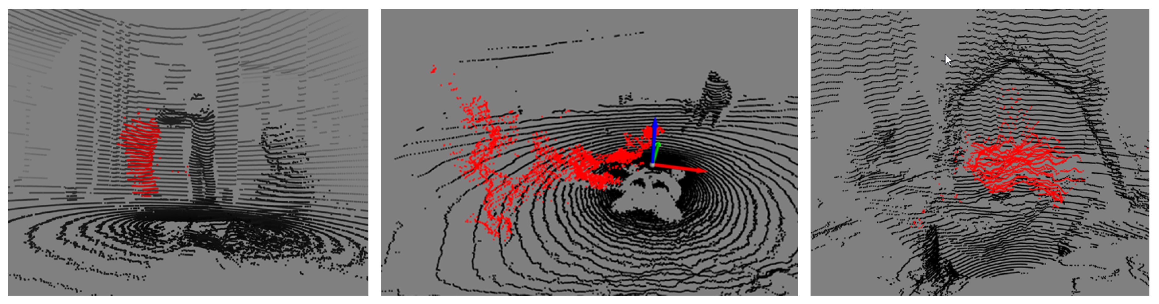
Table 1.
Comparison of key blocks of PointNet++ and reduced-PointNet++, highlighting the modifications in the number of sampled points and the configuration of the MLPs.
Table 1.
Comparison of key blocks of PointNet++ and reduced-PointNet++, highlighting the modifications in the number of sampled points and the configuration of the MLPs.
| Block | PointNet++ | reduced-PointNet++ |
| SA1 | 1024 pts, r=0.1, 32 nbr, MLP: [32, 32, 64] | 512 pts, r=0.1, 32 nbr, MLP: [16, 16, 32] |
| SA2 | 256 pts, r=0.2, 32 nbr, MLP: [64, 64, 128] | 128 pts, r=0.2, 32 nbr, MLP: [32, 32, 64] |
| SA3 | 64 pts, r=0.4, 32 nbr, MLP: [128, 128, 256] | - |
| SA4 | 16 pts, r=0.8, 32 nbr, MLP: [256, 256, 512] | - |
| FP4 | in_ch: 768, MLP: [256, 256] | - |
| FP3 | in_ch: 384, MLP: [256, 256] | - |
| FP2 | in_ch: 320, MLP: [256, 128] | in_ch: 96, MLP: [64, 32] |
| FP1 | in_ch: 128, MLP: [128, 128, 128] | in_ch: (32 + num_feats), MLP: [32, 32] |
| Conv1d | 128 → 128 | 32 → 32 |
| BatchNorm1d | 128 | 32 |
| Dropout | p=0.7 | p=0.7 |
| Conv1d (final) | 128 → num_classes | 32 → num_classes |
Table 2.
Variants of the proposed dust filtering method and the features used in each case. For simplicity in the notation, the temporal indices t are omited.
Table 2.
Variants of the proposed dust filtering method and the features used in each case. For simplicity in the notation, the temporal indices t are omited.
| Variant | Features Vector |
| SI | |
| STdm | |
| STdv | |
| STi | |
| SITdm | |
| SITdv | |
| SITi |
Table 3.
Overview of the UCHILE-Dust dataset subsets, including number of recordings, number of point clouds, total number of points, % of dust points, data format, and train/val/test split percentages.
Table 3.
Overview of the UCHILE-Dust dataset subsets, including number of recordings, number of point clouds, total number of points, % of dust points, data format, and train/val/test split percentages.
| Subset | Recordings | Point Clouds | Points | % Dust | Format | Train / Val / Test (%) |
| Interior 1 | 10 | 1,874 | 72,741,326 | 4.1% | PCAP | 82 / 09 / 09 |
| Interior 2 | 12 | 1,740 | 71,225,483 | 11.2% | PCAP | 70 / 15 / 15 |
| Exterior 1 | 10 | 1,529 | 45,311,889 | 3.2% | PCAP | 84 / 08 / 08 |
| Exterior 2 | 13 | 1,885 | 75,820,483 | 3.6% | PCAP | 66 / 17 / 17 |
| Carén | 13 | 7,089 | 234,929,532 | 8.1% | Rosbag | 46 / 26 / 28 |
Table 4.
Parameters used for the LIDROR method.
| Subset | N | |||
| Interior 1 | 90 | 0.001 | 0.01 | 4 |
| Interior 2 | 90 | 0.001 | 0.01 | 4 |
| Exterior 1 | 90 | 0.01 | 0.01 | 4 |
| Exterior 2 | 90 | 0.01 | 0.01 | 4 |
| Carén | 90 | 0.001 | 0.01 | 4 |
Table 5.
Results of dust-filtering using different methods in the Interior-1 dataset.
| Method | Learn. Rate | Accuracy (avg) |
Precision (dust) |
Recall (dust) |
F1-Score (dust) |
| SI | 0.008 | 0.79 | 0.12 | 0.93 | 0.22 |
| STdm | 0.008 | 0.87 | 0.17 | 1.00 | 0.29 |
| STdv | 0.008 | 0.86 | 0.17 | 0.99 | 0.29 |
| STI | 0.01 | 0.89 | 0.26 | 0.91 | 0.41 |
| SITdm | 0.01 | 0.86 | 0.17 | 0.97 | 0.29 |
| SITdv | 0.005 | 0.77 | 0.13 | 0.85 | 0.23 |
| SITi | 0.005 | 0.80 | 0.15 | 0.85 | 0.26 |
| LIDROR | - | 0.76 | 0.14 | 0.77 | 0.24 |
Table 6.
Results of dust-filtering using different methods in the Interior-2 dataset.
| Method | Learn. Rate | Accuracy (avg) |
Precision (dust) |
Recall (dust) |
F1-Score (dust) |
| SI | 0.008 | 0.94 | 0.53 | 0.94 | 0.68 |
| STdm | 0.008 | 0.92 | 0.6 | 0.88 | 0.71 |
| STdv | 0.01 | 0.84 | 0.5 | 0.74 | 0.59 |
| STI | 0.008 | 0.87 | 0.55 | 0.8 | 0.65 |
| SITdm | 0.008 | 0.94 | 0.68 | 0.91 | 0.78 |
| SITdv | 0.008 | 0.95 | 0.66 | 0.93 | 0.77 |
| SITi | 0.008 | 0.94 | 0.6 | 0.92 | 0.73 |
| LIDROR | - | 0.86 | 0.21 | 0.96 | 0.35 |
Table 7.
Results of dust-filtering using different methods in the Exterior-1 dataset.
| Method | Learn. Rate | Accuracy (avg) |
Precision (dust) |
Recall (dust) |
F1-Score (dust) |
| SI | 0.01 | 0.99 | 0.48 | 0.99 | 0.65 |
| STdm | 0.005 | 0.99 | 0.35 | 0.98 | 0.51 |
| STdv | 0.005 | 0.99 | 0.27 | 0.99 | 0.42 |
| STi | 0.005 | 0.97 | 0.46 | 0.95 | 0.62 |
| SITdm | 0.01 | 0.99 | 0.68 | 0.99 | 0.81 |
| SITdv | 0.005 | 0.99 | 0.54 | 0.98 | 0.70 |
| SITi | 0.01 | 0.99 | 0.51 | 0.98 | 0.67 |
| LIDROR | - | 0.91 | 0.03 | 0.98 | 0.06 |
Table 8.
Results of dust-filtering using different methods in the Exterior-2 dataset.
| Method | Learn. Rate | Accuracy (avg) |
Precision (dust) |
Recall (dust) |
F1-Score (dust) |
| SI | 0.005 | 0.98 | 0.38 | 0.99 | 0.55 |
| STdm | 0.01 | 0.98 | 0.35 | 0.99 | 0.52 |
| STdv | 0.01 | 0.97 | 0.36 | 0.97 | 0.53 |
| STi | 0.01 | 0.94 | 0.2 | 0.97 | 0.34 |
| SITdm | 0.005 | 0.98 | 0.38 | 0.99 | 0.55 |
| SITdv | 0.005 | 0.98 | 0.39 | 0.99 | 0.57 |
| SITi | 0.008 | 0.98 | 0.44 | 0.99 | 0.61 |
| LIDROR | - | 0.88 | 0.09 | 0.98 | 0.16 |
Table 9.
Results of dust-filtering using different methods in the Carén dataset. No odometry correction
Table 9.
Results of dust-filtering using different methods in the Carén dataset. No odometry correction
| Method | Learn. Rate | Accuracy (avg) |
Precision (dust) |
Recall (dust) |
F1-Score (dust) |
| SI | 0.005 | 0.98 | 0.61 | 0.98 | 0.75 |
| STdm | 0.01 | 0.95 | 0.43 | 0.96 | 0.60 |
| STdv | 0.01 | 0.95 | 0.47 | 0.94 | 0.62 |
| STi | 0.008 | 0.96 | 0.72 | 0.94 | 0.81 |
| SITdm | 0.01 | 0.98 | 0.6 | 0.98 | 0.74 |
| SITdv | 0.008 | 0.98 | 0.62 | 0.98 | 0.76 |
| SITi | 0.005 | 0.98 | 0.63 | 0.97 | 0.76 |
| LIDROR | - | 0.89 | 0.18 | 0.98 | 0.03 |
Table 10.
Results of dust-filtering using different methods with odometry correction in the Carén dataset.
Table 10.
Results of dust-filtering using different methods with odometry correction in the Carén dataset.
| Method | Learn. Rate | Accuracy (avg) |
Precision (dust) |
Recall (dust) |
F1-Score (dust) |
| SI | 0.005 | 0.98 | 0.61 | 0.98 | 0.75 |
| STdm | 0.008 | 0.96 | 0.56 | 0.95 | 0.70 |
| STdv | 0.008 | 0.95 | 0.41 | 0.96 | 0.58 |
| STi | 0.005 | 0.96 | 0.56 | 0.95 | 0.71 |
| SITdm | 0.005 | 0.98 | 0.64 | 0.98 | 0.77 |
| SITdv | 0.005 | 0.98 | 0.7 | 0.97 | 0.82 |
| SITi | 0.008 | 0.98 | 0.62 | 0.98 | 0.76 |
| LIDROR | - | 0.89 | 0.18 | 0.98 | 0.3 |
Disclaimer/Publisher’s Note: The statements, opinions and data contained in all publications are solely those of the individual author(s) and contributor(s) and not of MDPI and/or the editor(s). MDPI and/or the editor(s) disclaim responsibility for any injury to people or property resulting from any ideas, methods, instructions or products referred to in the content. |
© 2025 by the authors. Licensee MDPI, Basel, Switzerland. This article is an open access article distributed under the terms and conditions of the Creative Commons Attribution (CC BY) license (http://creativecommons.org/licenses/by/4.0/).
Copyright: This open access article is published under a Creative Commons CC BY 4.0 license, which permit the free download, distribution, and reuse, provided that the author and preprint are cited in any reuse.


