
Submitted:
12 September 2025
Posted:
15 September 2025
You are already at the latest version
Abstract
As machine learning and artificial intelligence are being integrated into cyber-physical systems, it is becoming important for engineers to know and understand these topics . In particular, sensor data is on the rise in these systems and therefore engineers need to understand which models are appropriate to time series sensor data and how signal processing can be used with them . The Center for Cyber-Physical Systems (CCPS) at the University of Georgia (UGA) is addressing these issues. Student researchers in the CCPS require skills in these areas. This paper demonstrates a machine learning framework for time series sensor data that can be used to quickly build, train, and test multiple models on CCPS testbed data. The framework is also a tool that can be used as a tutorial to help student researchers understand the concept required to be successful in the CCPS.
Keywords:
artificial intelligence
; digital signal processing
; false data injection attack
; machine learning
; sensor data
; time series
1. Introduction
Artificial intelligence and machine learning are becoming ubiquitous in modern industry [1], and is often referred to as Industry 4.0 [3,4,5]. In particular, the use of sensors in many fields, such as the Internet of Things, manufacturing, power, medical systems, digital twins, and other smart systems; sensor data is rapidly becoming the most common form of big data [2].
Industry has seen an increasing numbers of electronic control units (ECUs), programmable logic controllers (PLCs), and other types of programmable electronics have been deployed into cyber-physical systems. While such progress increased productivity and product quality, it also introduces vulnerabilities to both hardware and software.
In response to this issue, the Center for Cyber-Physical Systems (CCPS) is developing a testbed containing motors in order to collect realistic data for analysis and development of artificial intelligence and machine learning algorithms to solve fault and attack detection and diagnosis problems. The CCPS has also developed a smart plug, called ElectricDot, that can be used to easily integrate new devices into the testbed. Any device that uses a standard wall outlet may plug into an ElectricDot and be monitored by the testbed.
CCPS research requires skills in Machine Learning, Deep Learning, and Digital Signal Processing (DSP). Generally CCPS students are electrical or computer engineers, computer scientists, and occasionally statisticians. Most students have some background in signal processing or some background in machine or deep learning. Few have expertise in both. Thus, the CCPS students must learn these topics, generally via classes, while performing research. However, these topics are generally taught in classes that are independent of each other and their interrelation is not formally discussed. Thus, their interrelations have been discussed during lab hours or are done as independent study. Therefore the CCPS has started to formalize training and education of the topics.
The CCPS primary deals with sensor data gathered from cyber-physical systems and uses it with artificial intelligence and machine learning to perform research. While there are a multitude of definitions for cyber-physical systems (CPS) [6], the Sensorweb Lab defines them as any networked system that affects the physical world. Thus, the lab also primarily works with streaming data. Streaming data is a unique type of time series data in that it is continuously generated, can only be examined in one pass, and is prone to concept drift [7].
A need has arisen for CCPS researchers to have a framework that allows easy integration of data collection, algorithm training and testing. Additionally, the CCPS has developed smart plugs, called ElectricDot (eDots), to easily connect to electronic devices for monitoring their power electric waveform data. Thus this phase also includes adding the capability to easily connect models to eDots and other sensor devices. This paper presents a solution for these issues.
2. Materials and Methods
2.1. Background
Development of the CCPS testbed has proceeded in phases. Initially, a small prototype test bed involving toy motors was built as a proof of concept and is detailed in [8]. In this phase, a small information technology (IT) and operational technology (OT) network was created, with the motors at the OT level. A multilevel cyber attack was created. In short, an attacker was able to access the network via WiFi, scan the IT network for hosts, use a brute force password attack to break into Raspberry Pis with weak passwords and load an attack script. The script could then send commands to the motors on the OT network.
For defense, there were anomaly detection algorithms monitoring the network traffic, the system statistics of the Raspberry Pis, and the power usage of the motors via sensors. The goal was to demonstrate a multilevel attack on an OT/IT network and demonstrate multilevel detection.
The next phase involved moving from toy motors to industrial motors in a testbed. Details of this phase can be found in [9]. In this phase, the same basic attacks were implemented at the network level. However, a more sophisticated attack was developed for manipulating the industrial motors. Care was taken to ensure the attacks did not damage the motors. Compromised firmware and a control script, which was a compromised version of open source software for the control system vendor, were created in lieu of the basic attacks for the toy motors.
In both of these phases, live data was streamed to InfluxDB and Grafana was used for visualization. However, at these phases, data for training anomaly detection algorithms were simulated offline. Models were developed, trained, and tested offline as well.
This paper discusses the current phase of the CCPS testbed, the development of a framework. The framework is intended to help CCPS student researcher learn and understand relevant concepts to aid them in quickly training and testing models for to more comparison in CCPS research. The development of the framework was divided into to parts: the creation of its core functionalities along with a tutorial and the addition of the GUI with testbed integration via ElectricDots.
2.2. Previous Efforts with Tutorials
The Sensorweb Laboratory has made previous efforts to create tutorials to aid student researchers. These initially began assignments were lab members would create a small tutorial on a specific model. These were presented in lab meetings. They were later compiled and placed on a small website. However, tutorials were not standardize in format. Additionally, the code from one tutorial was not easily usable by another. Thus it was decided to consolidate the code into the framework and standardize the tutorial information into it as well.
2.3. CCPS Testbed Data Collection
The CCPS uses Message Queuing Telemetry Transport (MQTT) to send data and commands between sensors and systems. MQTT uses a publish/subscribe approach to handling messaging. Devices and apps subscribe to a topic to receive messages and publish to a topic to send. All messages and subscriptions are handled by an MQTT broker. InfluxDB, a free time series database, is used to store data. Grafana, a free tool, is used for data visualization of live streaming devices. Applications and smart devices used by the CCPS send data to the MQTT broker, which in turn forwards data to the InfluxDB servers. The testbed is located in a lab on UGA’s campus and is connected to the university’s secure network. The Grafana and InfluxDB servers reside in this network and are not accessible from outside the network.
2.4. ElectricDot
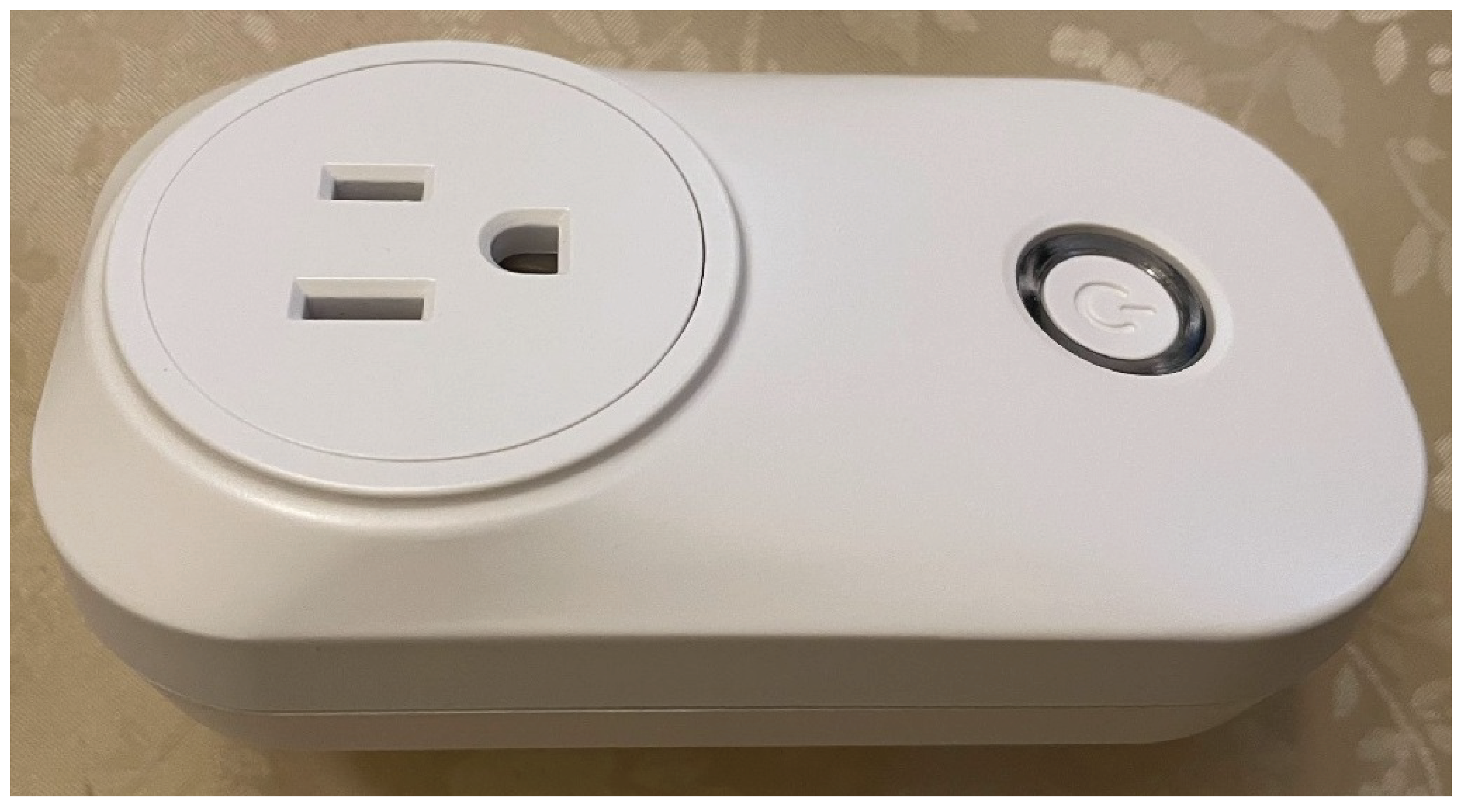
ElectricDot is a smart device designed to monitor the power electric waveform data of devices plugged into it. ElectricDot is plugged into a wall socket and the device that one intends to monitor is then plugged into the ElectricDot. Data is sent over WiFi via MQTT messages. The ElectricDot can be programmed to with a sample rate up to 10 kHZ. Additionally, various types of feature extraction; such as amplitude, frequency, and phase, angle; can be programmed as well. The ElectricDot was designed by CCPS in a separate project. Its purpose is to easily provide anomaly detection and diagnose for electric devices and networks. They allow for CCPS researchers to quickly add a power sensor to any device, including devices within the CCPS testbed. Thus, the SensorAI Framework is required to have the capability to interface with them.
Figure 1.
Picture of an ElectricDot smart plug.
2.5. Design Requirements
The projects and research discussed in this paper are the efforts of the Sensorweb Laboratory and the Intelligent Power Electronics and Electric Machine Laboratory. Both of which are members of the CCPS. Based on discussion with lab leaders and members, the following high-level requirements were determined for the framework:
- Must use Python
- Must focus on time series/sensor data.
- Minimize coding
- Easy to use
- Must assist in training and testing
- Must include metrics
- visualization of data and results
- Must have an accompanying tutorial
- Must include digital signal processing, classification, clustering, regression, and anomaly detection.
- Must have a Graphical User Interface
- Core functionality must be directly accessible
- Must enable smart device and historical data connectivity to models
2.6. Design Part 1: Core Functionality & Tutorial
The framework is built with Python. The primary interface for the framework is done via browser to a Streamlit web application server. Streamlit is an open source Python library for creating web applications. Note that the underlying code for the framework can be executed directly on a workstation with an Integrated Development Environment (IDE) or via a Google Colab TM notebook. It primarily uses the SciKit Learn,scikit-learn and SciPy,2020SciPy-NMeth packages, although others are used. Most models incorporated into the framework are SciKit Learn. Any model with Time Series in its name is from tslearn,JMLR:v21:20-091, which is an extension of SciKit Learn designed specifically for time series data. Users may upload their own data or generate data within the framework. Visualizations are done with matplotlib,Hunter:2007 and Plotly,plotly.
A complete list is contained in the requirement.txt file on the SensorAI GitHub [15]. The code is divided up by their core tasks. Digital Signal Processing, Classification, Clustering, Regression, and Anomaly Detection, and Utilities; refer to Table 1. Each machine learning module contains code for easy creation of pipelines and grid searches so that researchers can quickly train, test, and compare multiple models with minimal coding. Utilities contains the visualization and other miscellaneous functions the the core modules need. In general, a user will not need to access Utilities directly, but may do so if they choose.
For the core modules, there is very little coding required to build a model pipeline and place it in a grid search. Figure 2 show the code for setting up a grid search for three models, an Extra Trees, Random Forest, and an AdaBoost decision tree.
The rational for this organization was based on the CCPS need to ensure student researchers understand the core concepts. It also made integration of various algorithms easier, as models of each category generally rely on the same underlying utilities, such as metrics and visualization.
Most functions in DSP have a Show option, which is set to True or False, that allows the user to decide wether or not to plot the results of the operation. Thus users only need to set a variable plot instead of having to writer multiple lines of code to perform the same plotting.
2.6.1. Digital Signal Processing
The DSP module contains functions for all of the signal processing used in the framework. The groupings discussed in this section follow the general outline of the associated tutorial.
Wave generation: Wave generation allows users to create waves; such as sine, square, triangle; as well as pulses and chirps. Various types of noise can be added to these waves. Noise types include, but are not limited to white, flicker, impulse, and echo. There are also functions that allow users to automatically generate sets of waveforms, with or without noise, to create synthetic data sets that may be used for model training and testing as well as with tutorials. It also provides functions to generate seismocardiography (SCG) signal of a heartbeat, with or without respiration.
Filters & Signal Averaging: The module includes basic linear filters such as high-pass, low-pass, band-pass, and band-stop. It also includes more complex filters such as adaptive, moving average, and Kalman. Signal averaging contains several methods of dynamic-time-warping averaging techniques.
Time & Frequency Domains: The DSP module includes statistical moments, peak detection, envelope extraction, and waveform complexity measures. It also contains the Fast-Fourier Transform (FFT), the short time Fourier transform (STFT), and power spectral density functions. There are also functions to extract the average amplitude, frequency, and phase and of waveform as well as a function to calculate the Total Harmonic Distortion (THD) of a waveform.
Signal Decomposition: Within the module, there are functions to allow the user to break down (decompose) a signal into its fundamental parts and plot them. It includes Empirical Mode Decomposition (EMD), EMD variations, Singular Spectrum Analysis (SSA), and various Blind Source Separation techniques.
Wavelet Analysis & Transforms: Multiple type of wavelets and chirplets are available in the module. Additional, the following wavelet based transforms are in this module: Continuous Wavelet Transform (CWT), Polynomial Chirplet Transform (PCT), Wigner-Ville Distribution (WVD), and SynchroSqueezing Transform (SST).
2.6.2. Classification
This module contains all the classification models available in the framework. It also contains the functions for streamlining pipeline building and grid searches. The groupings discussed in this section follow the basic outline of the associated tutorial. These models can also be used for anomaly detection (see the Detection section below.).
Decision Trees, Bagging & Boosting: In addition to basic decision trees, the framework includes several tree based bagging methods: Random Forests and Extra Trees. It includes two tree specific boosting methods: Gradient Boosting and Histogram Gradient Boosting. It includes a generic bagging model that can create ensembles of other model types called Bagging. Lastly, it includes a generic boosting model that can boost other model types called AdaBoost.
Nearest Neighbors: This module contains several nearest neighbor based models. They are K Nearest Neighbors (KNN), Nearest Centroid, Radius Nearest Neighbors, and Time Series K Nearest Neighbors (TS KNN).
Support Vector Classifiers: The framework contains three support vector based models: Support Vector, Nu Support Vector, and Time Series Support Vector.
Other Classifiers: There are multiple other classifier models available, which include but is not limited to: Discriminant Analysis, Early Classifiers, and Naive Bayes classifiers.
2.6.3. Clustering
This module contains all the clustering models available in the framework. It also contains the functions for streamlining pipeline building and grid searches. The groupings discussed in this section follow the basic outline of the associated tutorial.
Hierarchical Clustering: In the tutorial, Hierarchical Clustering is used as an introduction to clustering as these models are simple. Agglomeration and Feature Agglomeration are available in the framework.
K-Means: K-Means is another easy clustering model to understand. The framework includes the following K means based variants: K-Means, Bisecting K-Mean, Mini-Batch K-Means, Time Series K-Means, and K-Shape.
Density Based Clustering: The density based clustering algorithms available in the framework are Mean Shift, Density-Based Spatial Clustering of Applications with Noise (DBSCAN), and Ordering Points To Identify the Clustering Structure (OPTICS)
Spectral Clustering: Spectral Clustering is the only other clustering algorithm currently available in the framework.
2.6.4. Detection
Unsupervised anomaly detection is divided into Outlier Detection and Novelty Detection. In outlier detection, the goal is to identify anomalous data within your data set. Usually with the intent to remove them. In novelty detection, the goal is to build a model that can label future data inputs as either normal or anomalous.
In this framework, supervised anomaly detection is part of classification. Any classification method can be an anomaly detection method if the normal condition is one class and all other conditions are treated as anomalous.
Outlier Detection: Unsupervised outlier detection is contained in the Detection module. The detectors are Local Outlier Factor, and Elliptic Envelope.
Novelty Detection: Unsupervised novelty detection is contained in the Detection module. The detectors are One-Class Support Vector Machine, One-Class Support Vector Machine with Stochastic Gradient Descent, Isolation Forests, and Local Outlier Factor for Novelty Detection.
2.6.5. Regression
This module contains all the regression models available in the framework. It also contains the functions for streamlining pipeline building and grid searches. The groupings discussed in this section follow the basic outline of the associated tutorial. When using the tutorial, regression is general used first since it contains discussions on probability, distributions, loss functions, cross-validation, and regularization.
General Linear Models: The general linearized models available in the framework are: Linear, Gamma, Poisson, and Tweedie.
LARS & LASSO: Least Angle Regression Shrinkage (LARS) and Least Absolute Shrinkage and Selection Operator (LASSO) are included together. There are several variants of the models included in the the framework: LARS, LARS with Cross Validation, LASSO, LASSO with Cross Validation, LassoLars, and LassoLars with Cross-Validation.
Ridge: The Ridge based models available are Ridge, Ridge with Cross Validation, and Bayesian Ridge.
Elastic Net Regularization: Elastic Net Regularization (Elastic-Net) is a combination of LARS and Ridge. There a several variants of Elastic-Net available: Elastic-Net, Elastic-Net with Cross Validation, Multitask Elastic-Net, and Multitask Elastic-Net with Cross Validation.
Support Vector Regression: The support vector regressor models include are: Linear Support Vector, Nu Support Vector, and Time Series Support Vector.
Other Regression Methods: The list of other regressor available includes, but is not limited to Huber, TheilSen, Random Sample Consensus (RANSAC), Time Series KNN regressor, and Quantile.
2.6.6. Utilities
This module mostly contains the various plotting functions and some metric calculations. It has a few miscellaneous functions that do not fall into any of the other categories in the framework. The plotting functions primarily used are for confusion matrices and waveform data display.
2.6.7. Framework Tutorial
Each of the core machine learning modules of the framework has a companion tutorial on how to use it; refer to Table 2. Clustering and Unsupervised Anomaly Detection are combined into the Unsupervised tutorials. Supervised Anomaly Detection is covered under the Classification tutorials. The tutorial include overviews of the concepts and algorithms of the include machine learning algorithms. There is a set of slides and a Jupyter notebook with executable framework code for each module.
The general outline of each tutorial follows the topics grouped in the discussion of each module in the code design section. The outline below highlights the main topics on which each tutorial is focused.
- DSP: wave generation, noise, filters, transforms, decomposition, power spectral density, wavelet analysis & transforms
- Classification: decision trees, nearest neighbors, support vector machines, bagging, boosting, others
- Clustering: hierarchical, k-means, k-shape, density based, spectral, others
- Anomaly Detection: outlier vs novelty detection, isolation forests, local outlier factor, others
- Regression: generalized linear models, lars, lasso, ridge, elastic nets, nearest neighbors, support vector machines, others
2.7. Design Part 2: Graphical User Interface & Testbed Integration
A free python package, Streamlit, was chosen for the GUI. Streamlit is for building graphical interfaces to python code that are accessed via a web browser. It was chosen for ease of use and minimization of coding.
The graphical user interface for the framework follows the basic architecture of the core framework code. There are pages for digital signal processing, classification, clustering, detection, and regression. Additionally, there are pages for loading and generating data, downloading data from InfluxDB and running it through and existing model, and one for connecting an active ElectricDots to a trained model and sending model outputs to the MQTT broker for forwarding to the appropriate InfluxDB server. It also allows for the connecting of a model to historical data from the InfluxDB server. Lastly, there is a page for the tutorials. The SensorAI Framework is integrated with the motor testbed as shown in Figure 3 below.
The framework GUI may be ran via the Homepage.py file. This files sets the basic layout and color schemes. Each page, except for the Device Connector and Historical Data Connector, has an associated python file that contains most of the related GUI functionality. This is done to avoid overly large files for ease of maintenance and understanding. The code design for the framework is illustrated in Figure 4. Within the testbed, the framework is hosted on a server running the Streamlit code.
2.7.1. Data
The Data page is the second in the framework. Here, users can choose to load data from numpy data (.npy) files or a comma-separated values (.csv) files. Alternate the may generate a single waveform or a set of multiple waveforms. Lastly, users may generate Seismocardiography data. Either a single example or a data set of randomly generated ones. The Data page can be seen in Figure 5.
2.7.2. Digital Signal Processing
The DSP page contains all the functions for digital signal processing. It is segregated by sub menus: Noise, Filters, Decomposition, Time Domain Features, Transforms, and Misc. The DSP menu can be seen in Figure 6.
2.7.3. Classification
The Classification page offers several models that users may train and test. They may use their own data or data generated by the framework. Related models are grouped in columns. The Classification page is shown in Figure 7. Note that any classification model may be used as novelty detection in the case of having training data with normal and abnormal labels.
2.7.4. Clustering
The Clustering page offers several models that users may train and test. They may use their own data or data generated by the framework. Related models are grouped in columns. The Clustering page is shown in Figure 8.
2.7.5. Detection
The Detection page has two sub-menus, Novelty and Outlier. These menus contain a few models that are specific to these tasks. The Detection page is shown in Figure 9.
2.7.6. Regression
The Regression page offers several models that users may train and test. They may use their own data or data generated by the framework. Related models are grouped in columns. The Regression page is shown in Figure 10.
2.7.7. Device Connector
The Device Connector page allows the user to connect an trained model to an online ElectricDots. Models trained and saved by the framework are pickled and an accompanying yaml file with model information is generated. User may connect any of there own models, so long as it is in pickled format and the user has created an appropriately structured accompanying yaml file. The page is shown in Figure 11. When connecting a model to an ElectricDot, a separate processes is opened and the main_ai_mqtt.py script is automatically ran with the appropriate settings. A separate terminal window opens and displays any text output. The connection can be monitored from this terminal window.
2.7.8. Historical Download
The Historical page allows users to download and pass historical data from the InfluxDB server to a model of their choosing. As with the the previous section, the models must be pickled and have their accompanying yaml file. This page is shown in Figure 12. When connecting a model to historical InfluxDB data, a separate processes is opened and the main_ai_influx.py script is automatically ran with the appropriate settings. A separate terminal window opens and displays any text output. The connection can be monitored from this terminal window.
2.7.9. Tutorials
The tutorials page includes menus for the slides that may be viewed on the website and an option to open the Jupyter notebook tutorials in GitHub TM in a separate browser tab. All tutorial notebooks are setup to open them in Google Colab TM. See Figure 13
3. Results
The framework prototype was first used as a teaching aid in the University of Georgia (UGA) Spring 2024 class, Principles of Cyber-Physical Systems. Using feedback from students and the instructor, the framework design and the tutorials were refined and improved. The framework was used by some of the students to complete homework and project assignments. The framework was used again during in the Spring 2025 semester of the same class, to further refine and improve the framework and associated tutorials.
To demonstrate the effectiveness of the framework, a comparison of machine learning models utilized within the framework was performed. Training data was utilized from simulations in previous experiments of the testbed.
3.1. Data
The dataset used in this study was generated using a real-world cyber-physical security testbed specifically designed for networked electric drive systems. This testbed, referred to as the CCPS testbed, integrates four electric machine drives—comprising two induction machines and two permanent magnet synchronous machines—each controlled by a TI C2000 TMS320F28335 micro-controller operating under a field-oriented control (FOC) strategy. These drives are embedded within a hybrid IT/OT network environment to emulate realistic control and communication scenarios.
To create high-fidelity cyber-attack data, predefined false data injection attacks (FDIAs) and step-stone attacks through software back doors embedded in the digital signal controllers were created and implemented. The FDIAs target current feedback and speed reference variables, introducing precise distortions in the control loop. These attacks were activated under controlled conditions to maintain system safety while ensuring authentic physical responses. Data reflecting system behavior under normal operation and various attack conditions were collected in real time using NI cDAQ-9132 hardware and streamed to an InfluxDB time-series database.
The sample rate was 10k Hz. Data was collected at varying motor speeds: 400, 800, 1200, 1300, 1600 rpms. Data was collected with and without loads (1V, 2V, 3V) at each speed. The FDIA attacks injected a constant into one or two of the three phase current readings of the motor’s control unit. FDIA type "1" injected a constant into Phase A. FDIA type "2" injected a constant into both Phase A and Phase B. The constant values injected were a percentage of the amplitude added to the actual amplitude and varied as follows: 0.5, 1.0, 2.0, 2.5, 3.0, 3.5, 4, 4.5, and 5 percent.
Sensor readings from the motors, DC bus, and point of common coupling (PCC) were integrated via a dedicated sensor board, enabling the collection of diverse electrical signatures across all scenarios. The dataset was further enriched with synchronized waveform snapshots and labeled attack scenarios, facilitating both machine learning-based fault classification and cyber-attack diagnostics.
3.2. Framework Model Comparisons
From the data described above, only the single-phase current at the PCC was used. The data is divided into windows, with each window containing the raw single phase current waveform data. Each window was down sampled from 10k Hz to 4k Hz. To increase the number of windows within the data set, white noise was added to each window and added to the data via the framework. This was done six times for each window in the original data. Next, the framework was used to extract the Amplitude, Frequency, and Phase Angle of each window. These feature data were used for the model comparisons. There were 63 windows in the original data. After adding noisy windows there are 441. There are 91 normal cases, 140 FDIA 1 cases, and 210 FDIA 2 cases.
For the model comparisons, this data was used to test and train a version of each classification model in the framework. Each model was run through a grid search with varying assignments of hyperparamaters. The best models from each run exhibiting an accuracy of 99% were kept for the next series of runs. These model’s hyperparamaters where given more assigned values to run through the grid search. The experiment was performed ten times and the results were tracked and compared. The models that performed the best were Extra Trees, Random Forests, K Nearest Neighbors (KNN), and Time Series K Nearest Neighbors (TS KNN). Note that TS KNN is from the tslearn which is included in the framework.
The following models were used in the final comparison: Decision Trees, AdaBoost (with decision trees), Bagging (with decision trees), Extra Tress, Gradient Boosting, Histogram Gradient Boosting, K Nearest Neighbors (KNN), Random Forests, and Time Series K Nearest Neighbors (TS KNN). Note that all of the listed methods are tree ensembles except for the Decision Tree, KNN, and TS KNN.
Ensembles are a collection of models. Each model within and ensemble is called an estimator. Bagging models are composed of multiple estimators working in parallel on the same input. Voting is performed on the output of all estimators, which can be weighted or unweighted. Boosting models are simply serialized ensembles. Each estimator make decisions based on the output of the prior estimator, with the last estimator making the final decisions. The bagged tree models are the Bagging, Extra Trees, and Random Forests. The boosted models are AdaBoost, Gradient Boosting, and Histogram Gradient Boosting.
For all of the tree based models the grid search was performed over a tree maximum depth of 3, 5, 25, 50. The maximum depth of a decision tree is the number of nodes to pass through before reaching the deepest leaf in the tree. The number of estimators in the ensembles chosen for the grid search were 10, 50, and 100.
Nearest neighbor models assume that like things exist in close proximity to each other. The KNN model compares a new input to all pervious assigned inputs takes the mode of the k closet inputs’ assigned labels. Close being a distance measure, usually Euclidean distance. The KNN and TS KNN are essentially the same models. However, the TS KNN has similarity measure call Global Alignment Kernel (GAK) that is specific to time series data [16]. For these two modes a grid search for k was performed over the following values: 3, 5, and 10.
During the comparisons, several metrics were tracked in order to show the utility of the framework. The metrics were accuracy, precision, recall, and F1 score. Note the comparisons were was run in Google Colab TM using L4 Graphics Processing Unit (GPU).
4. Discussion
The framework was successfully demonstrated using testbed data for model comparison and evaluation. Using the framework, models were created that could correctly classify normal operation and FDIA attacks on the motor operating at different speeds. The best performing models after feature extraction were the tree based models and K Nearest Neighbors and its time series version.
Additionally, its tutorial component was successfully used as a teaching to in a UGA graduate class. Some students used the frameworks for relevant projects. Feedback was positive from both classes in which the framework was used.
However, it is currently limited to machine learning models that have been integrated into the framework. Additionally, it is not yet fully integrated into the CCPS testbed. Lastly, the speed at which the framework trains and test models is limited by a student researches access to GPUs.
4.1. Future Work
The next step is to fully integrate the framework with the testbeds, sensors, and data infrastructure. This will include linking the framework to a Message Queuing Telemetry Transport (MQTT) broker system and CCPS testbed databases. This will allow for models designed and tested within the framework to be quickly deployed to live data streams from sensors within the testbed. Additionally, a graphical user interface is planned for incorporation with the framework.
Author Contributions
For research articles with several authors, a short paragraph specifying their individual contributions must be provided. The following statements should be used “Conceptualization, S.C. and Y.Y.; methodology, S.C.; software, S.C.; validation, S.C. and W.S.; formal analysis, S.C.; investigation, S.C., H.Y. and S.W.; resources, S.C., J.Y. and W.S.; data curation, H.Y. and S.W; writing—original draft preparation, S.C.; writing—review and editing, S.C., H.Y., S.W, and W.S.; visualization, S.C.; supervision, J.Y., P.M, and W.S; project administration, J.Y. and W.S.; funding acquisition, J.Y., P.M. and W.S. All authors have read and agreed to the published version of the manuscript.
Funding
Our research is partially supported by NSF-1940864, NSF-2019311, NSF-2324389, NSF-2312974, Georgia Research Alliance, DOE-EE0009026, DOD-FA8571-21-C-0020, NIH-1R01HL172291-01.
Data Availability Statement
We encourage all authors of articles published in MDPI journals to share their research data. In this section, please provide details regarding where data supporting reported results can be found, including links to publicly archived datasets analyzed or generated during the study. Where no new data were created, or where data is unavailable due to privacy or ethical restrictions, a statement is still required. Suggested Data Availability Statements are available in section “MDPI Research Data Policies” at https://www.mdpi.com/ethics.
Conflicts of Interest
The authors declare no conflict of interest.
Abbreviations
The following abbreviations are used in this manuscript:
| CCPS | Center for Cyber-Physical Systems |
| CWT | Continuous Wavelet Transform |
| DBSCAN | Density-Based Spatial Clustering of Applications with Noise |
| DSP | Digital Signal Processing |
| ECU | Electronic Control Unit |
| eDOt | ElectricDot |
| Elastic-Net | Elastic-Net Regularization |
| EMD | Empirical Mode Decomposition |
| FDIA | False Data Injection |
| FFT | Fast-Fourier Transform |
| FOC | Field-Orient Control |
| GAK | Global Alignment Kernel |
| GPU | Graphics Processing Unit |
| GUI | Graphical User Interface |
| IT | Information Technology |
| KNN | K Nearest Neighbors |
| LARS | Least Angle Regression Shrinkage |
| LASSO | d Least Absolute Shrinkage and Selection Operator |
| MQTT | Message Queuing Telemetry Transport |
| OPTICS | Ordering Points To Identify the Clustering Structure |
| OT | Operational Technology |
| PCC | Point of Common Coupling |
| PCT | Polynomial Chirplet Transform |
| RANSAC | Random Sample Consensus |
| SCG | Seismocardiography |
| SSA | Singular Spectrum Analysis |
| SST | SynchroSqueezing Transform |
| STFT | Short Time Fourier Transform |
| THD | Total Harmonic Distortion |
| TS KNN | Time Series K Nearest Neighbors |
| UGA | University of Georgia |
| WVD | Wigner-Ville Distribution |
References
- Weerts, H.J.P.; Pechenizkiy, M. Teaching responsible machine learning to engineers. In Proceedings of the The Second Teaching Machine Learning and Artificial Intelligence Workshop. PMLR, 2022, pp. 40–45.
- Selmy, H.A.; Mohamed, H.K.; Medhat, W. A predictive analytics framework for sensor data using time series and deep learning techniques. Neural Computing and Applications 2024, 36, 6119–6132.
- Lasi, H.; Fettke, P.; Kemper, H.G.; Feld, T.; Hoffmann, M. Industry 4.0. Business & information systems engineering 2014, 6, 239–242.
- Lu, Y. The current status and developing trends of industry 4.0: A review. Information Systems Frontiers 2025, 27, 215–234.
- Ambadekar, P.K.; Ambadekar, S.; Choudhari, C.; Patil, S.A.; Gawande, S. Artificial intelligence and its relevance in mechanical engineering from Industry 4.0 perspective. Australian Journal of Mechanical Engineering 2025, 23, 110–130.
- Putnik, G.D.; Ferreira, L.; Lopes, N.; Putnik, Z. What is a Cyber-Physical System: Definitions and Models Spectrum. Fme Transactions 2019, 47.
- Chen, Y.; Tu, L. Density-based clustering for real-time stream data. In Proceedings of the Proceedings of the 13th ACM SIGKDD international conference on Knowledge discovery and data mining, 2007, pp. 133–142.
- Coshatt, S.J.; Li, Q.; Yang, B.; Wu, S.; Shrivastava, D.; Ye, J.; Song, W.; Zahiri, F. Design of cyber-physical security testbed for multi-stage manufacturing system. In Proceedings of the GLOBECOM 2022-2022 IEEE Global Communications Conference. IEEE, 2022, pp. 1978–1983.
- Yang, H.; Yang, B.; Coshatt, S.; Li, Q.; Hu, K.; Hammond, B.C.; Ye, J.; Parasuraman, R.; Song, W. Real-world Cyber Security Demonstration for Networked Electric Drives. IEEE Journal of Emerging and Selected Topics in Power Electronics 2025, pp. 1–1. https://doi.org/10.1109/JESTPE.2025.3550830.
- Pedregosa, F.; Varoquaux, G.; Gramfort, A.; Michel, V.; Thirion, B.; Grisel, O.; Blondel, M.; Prettenhofer, P.; Weiss, R.; Dubourg, V.; et al. Scikit-learn: Machine Learning in Python. Journal of Machine Learning Research 2011, 12, 2825–2830.
- Virtanen, P.; Gommers, R.; Oliphant, T.E.; Haberland, M.; Reddy, T.; Cournapeau, D.; Burovski, E.; Peterson, P.; Weckesser, W.; Bright, J.; et al. SciPy 1.0: Fundamental Algorithms for Scientific Computing in Python. Nature Methods 2020, 17, 261–272. https://doi.org/10.1038/s41592-019-0686-2.
- Tavenard, R.; Faouzi, J.; Vandewiele, G.; Divo, F.; Androz, G.; Holtz, C.; Payne, M.; Yurchak, R.; Rußwurm, M.; Kolar, K.; et al. Tslearn, A Machine Learning Toolkit for Time Series Data. Journal of Machine Learning Research 2020, 21, 1–6.
- Hunter, J.D. Matplotlib: A 2D graphics environment. Computing in Science & Engineering 2007, 9, 90–95. https://doi.org/10.1109/MCSE.2007.55.
- Inc., P.T. Collaborative data science, 2015.
- Song, W.; Coshatt, S.; Zhang, Y.; Chen, J. Sensor Data Science and AI Tutorial, 2024.
- Cuturi, M. Fast global alignment kernels. In Proceedings of the Proceedings of the 28th international conference on machine learning (ICML-11), 2011, pp. 929–936.
Figure 2.
An example of framework code. An extra trees, random forest, and ada boosted decision tree classifiers are created and then placed in a grid search. Note that hyperparameter values for the grid search are placed in lists.
Figure 2.
An example of framework code. An extra trees, random forest, and ada boosted decision tree classifiers are created and then placed in a grid search. Note that hyperparameter values for the grid search are placed in lists.
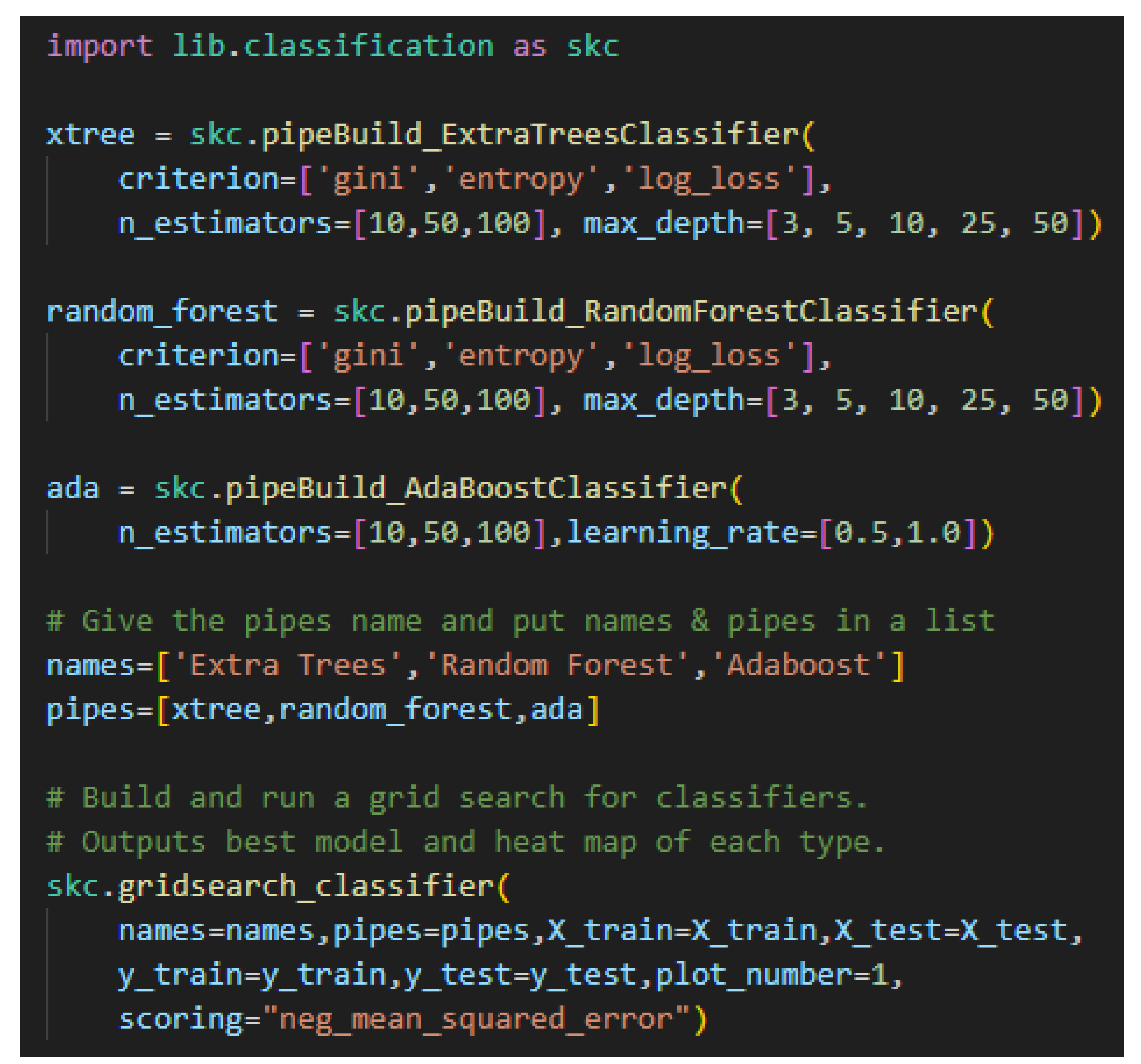
Figure 3.
SensorAI Framework & Testbed Integration: The SensorAI Framework is hosted on a server that resides in UGA’s secure network. All PCs, servers, and brokers also hosted on UGA’s secure network. The motors, the PCs used for motor control, and the eDots are all physically located in the same lab on campus. Note that the eDots smart plug is connected to the PCC that all four motors are connected to.

Figure 4.
Framework Code Design: Homepage.py is the main Streamlit page. The functionality is divided into nine subpages. Each subpage is title with a number followed by an underscore. Streamlit uses this numbering for page ordering. Each page is a graphical interface to the underlying functional code or to the tutorials.
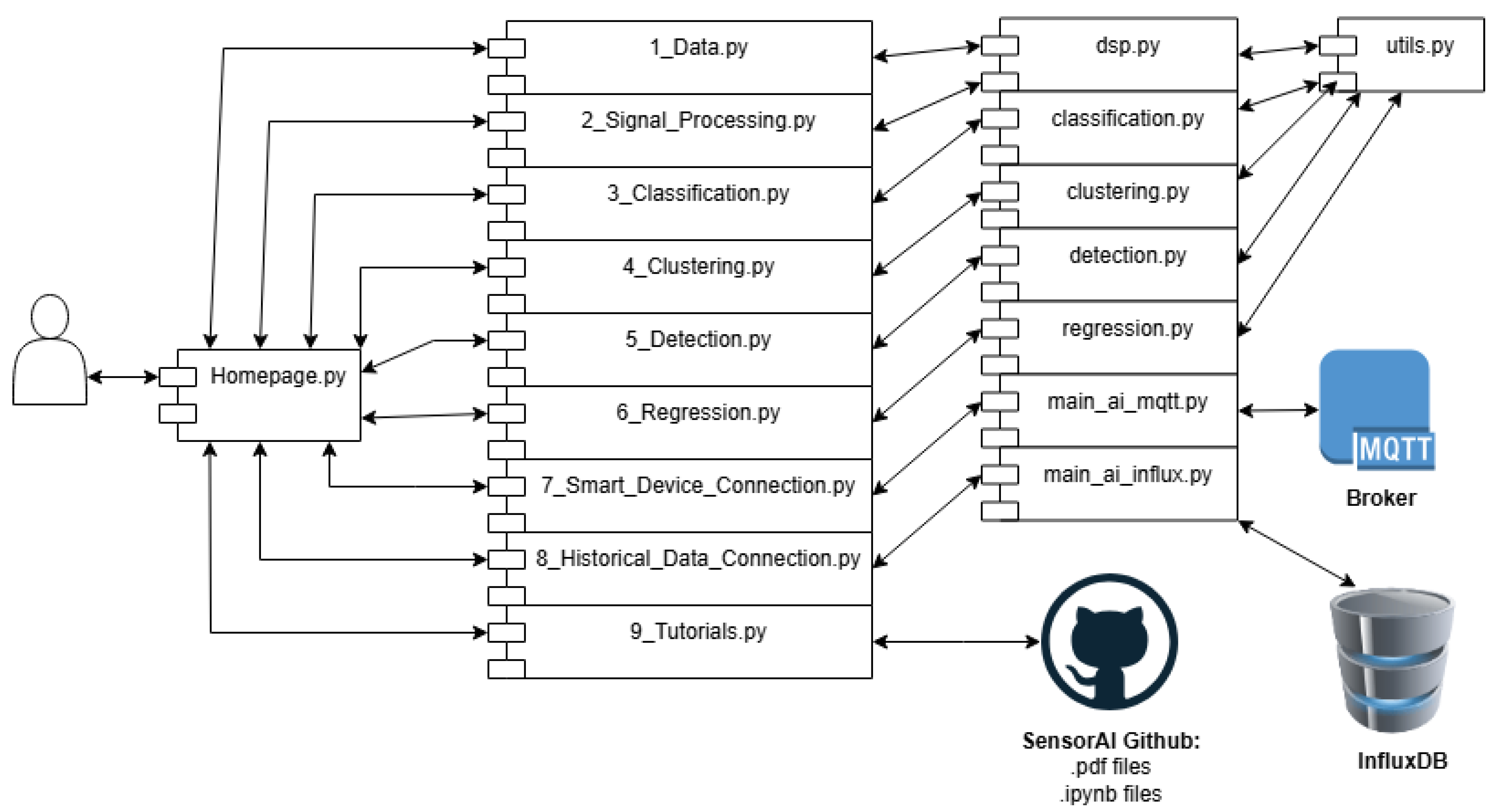
Figure 5.
The image is of the Data Page after a demo dataset has been loaded. Note that options are selected in the left sidebar. Once data is selected, a preview of the first five entries is displayed. A data summary is displayed below it. While not shown in the screenshot, the first row of data is also plotted.
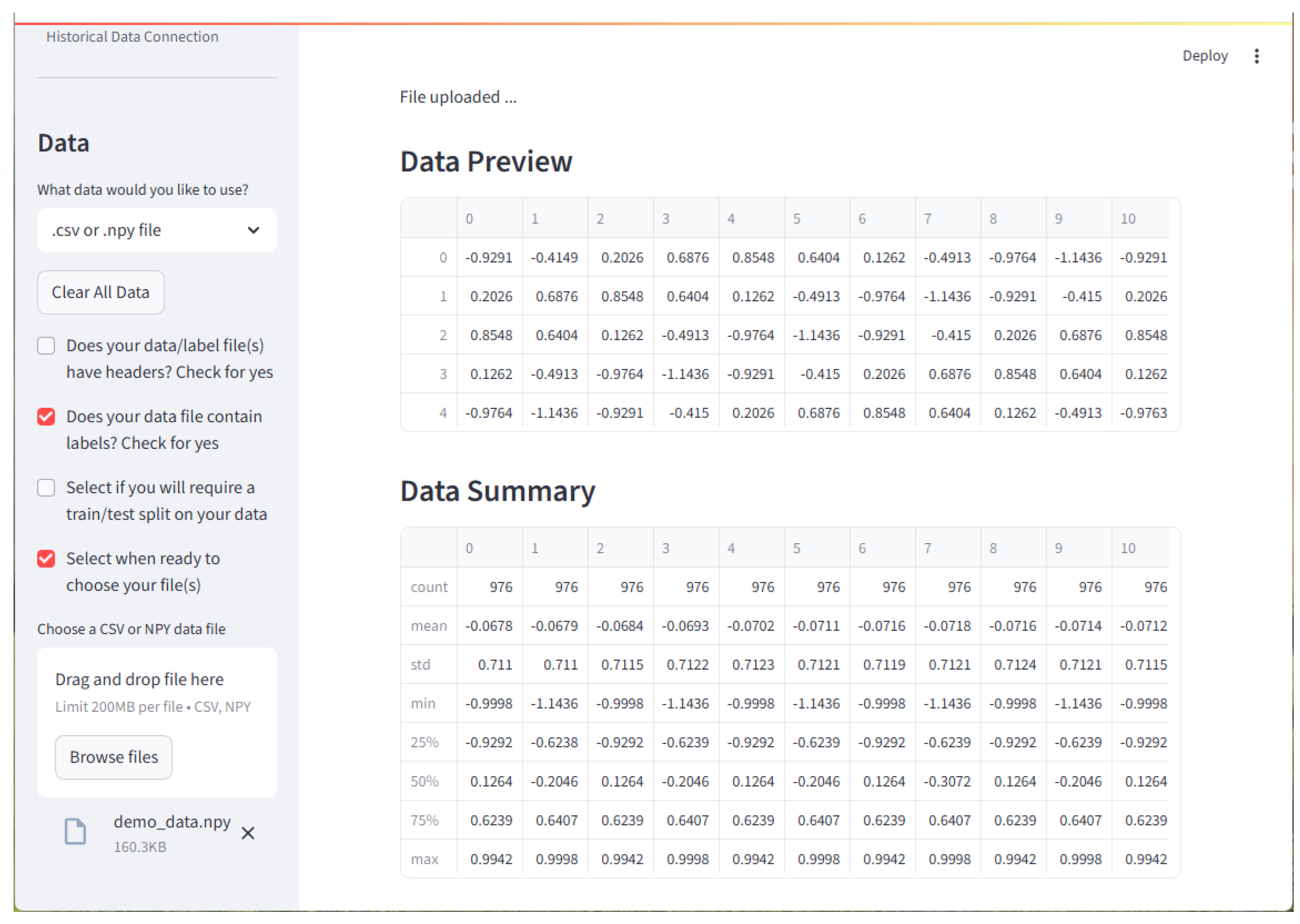
Figure 6.
The Signal Processing Page is where digital signal processing techniques may be applied to a loaded dataset. Here, basic gaussian white noise is added to the demonstration dataset. Note that the first entry of the dataset is plotted. Both the original signal and the signal with added noise are shown.
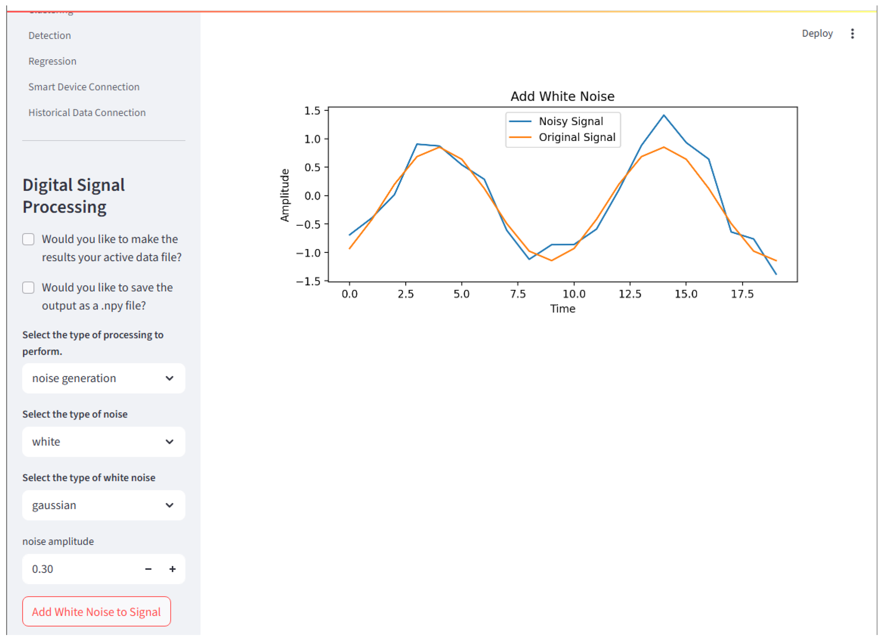
Figure 7.
Classification Page is where classification algorithms may be created and queued to run on a loaded dataset. Multiple inputs for each hyperparameter of multiple models may be created and run through a grid search. The best model of each type place in the queue will have results displayed. Here, a confusion matrix and the first three samples of each class are displayed. Note that plots in black are correctly classified and those in red are incorrectly classified.
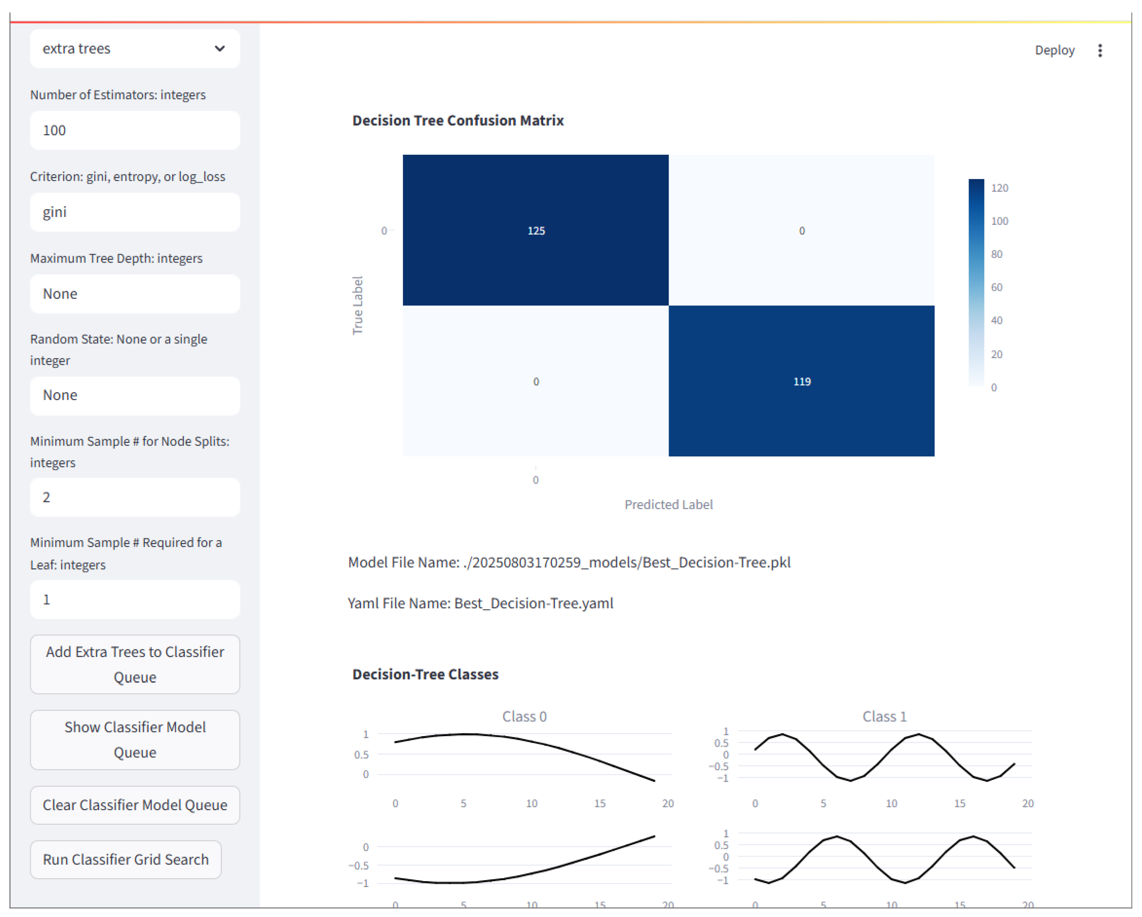
Figure 8.
Classification Page is where clustering algorithms may be created and queued to run on a loaded dataset. Multiple inputs for each hyperparameter of multiple models may be created and run through a grid search. The best model of each type place in the queue will have results displayed. Here, the first three samples of each cluster are displayed. Note that plots in black are correctly clustered and those in red are incorrectly clustered.
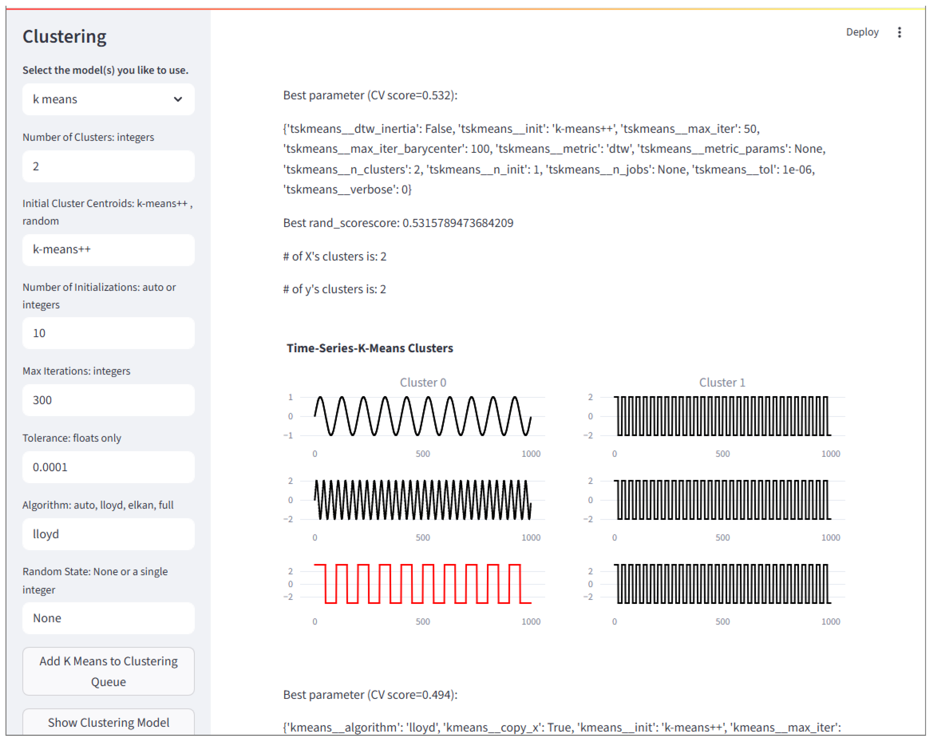
Figure 9.
The Detection Page is where outlier and novelty detection algorithms may be created and queued to run on a loaded dataset. Multiple inputs for each hyperparameter of multiple models may be created and run through a grid search. The best model of each type place in the queue will have results displayed. Here, a confusion matrix and the first three samples of each class are displayed, where the first column is normal (sine waves) and the second column is abnormal (square waves). Note that plots in black are correctly identified and those in red are incorrectly identified.
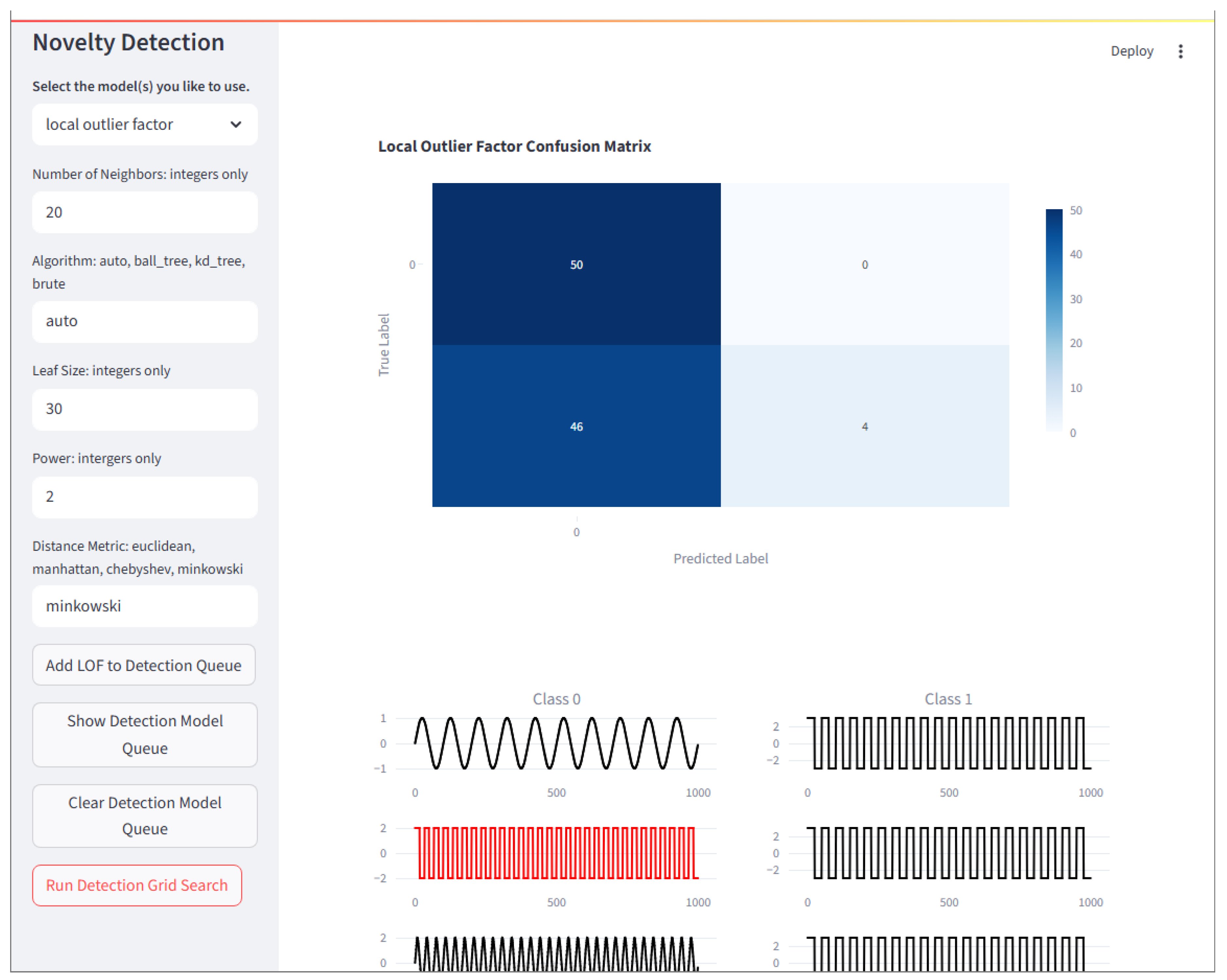
Figure 10.
The Regression Page is where regression algorithms may be created and queued to run on a loaded dataset. Multiple inputs for each hyperparameter of multiple models may be created and run through a grid search. The best model of each type place in the queue will have results displayed. Here, a scatterplot is displayed. Note that predicted values are blue and the labels (true values) are red.
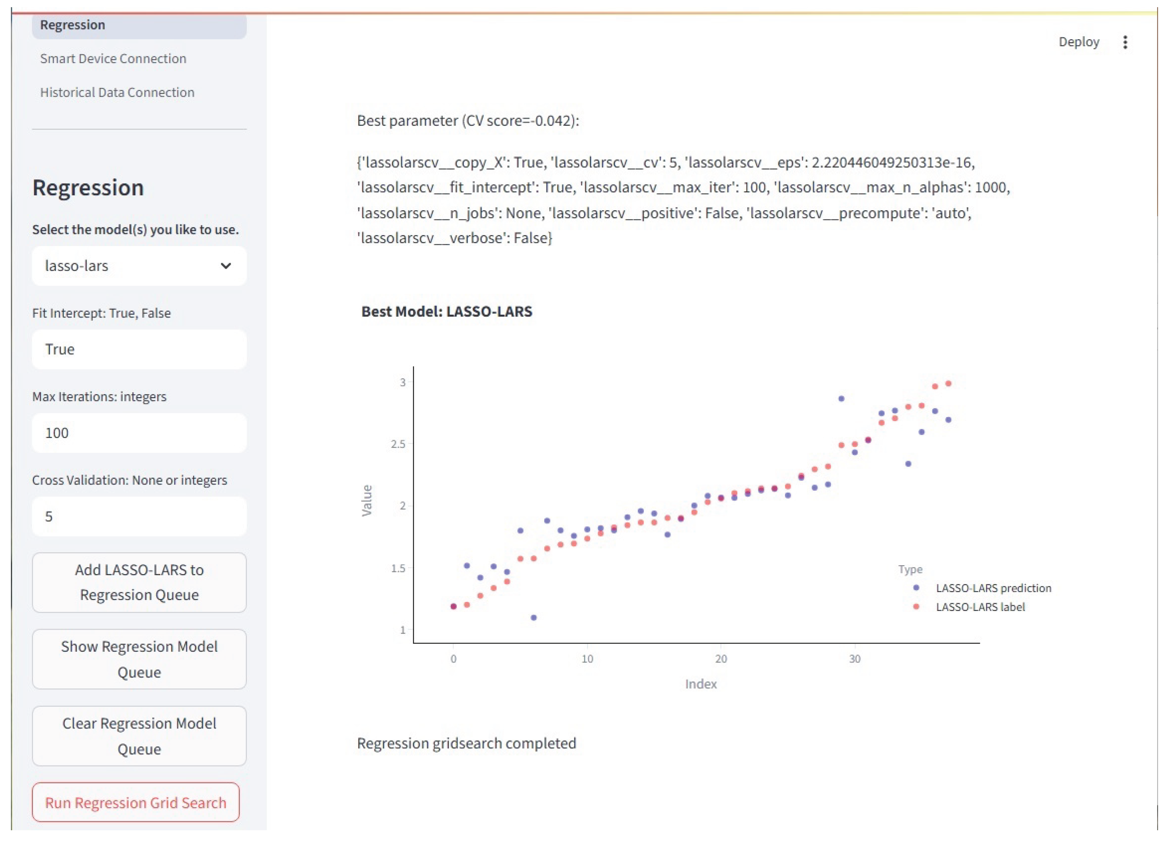
Figure 11.
The Device Connector Page is where a trained model may be connected to a live ElectricDot (or other smart device) data stream. The model and the smart device each have an associate .yaml file that contains the information that the framework needs to make the connection. Based on the information in the .yaml file, the model output is automatically routed to the appropriate InfluxDB server and table. From there, Grafana may be used to visualize the smart device and model outputs in real time.
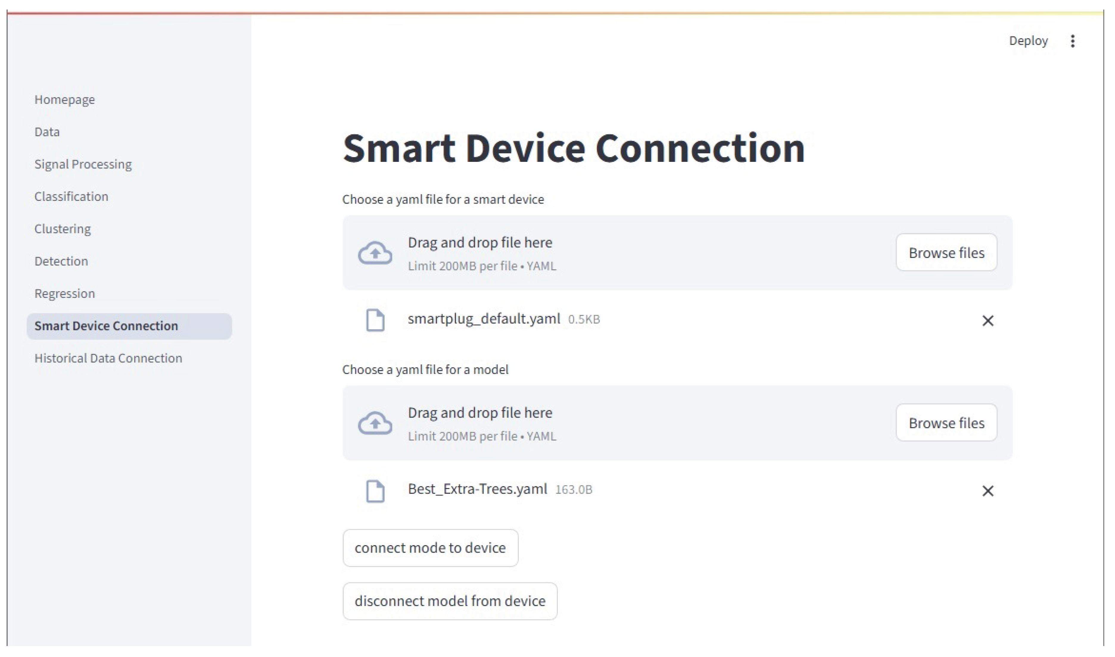
Figure 12.
The Historical Data Page is where a trained model may be connected to historical data stored in the testbeds InfluxDB server. The historical data is queried and sent to the model. It otherwise functions the same as the Device Connector discussed above.
Figure 12.
The Historical Data Page is where a trained model may be connected to historical data stored in the testbeds InfluxDB server. The historical data is queried and sent to the model. It otherwise functions the same as the Device Connector discussed above.
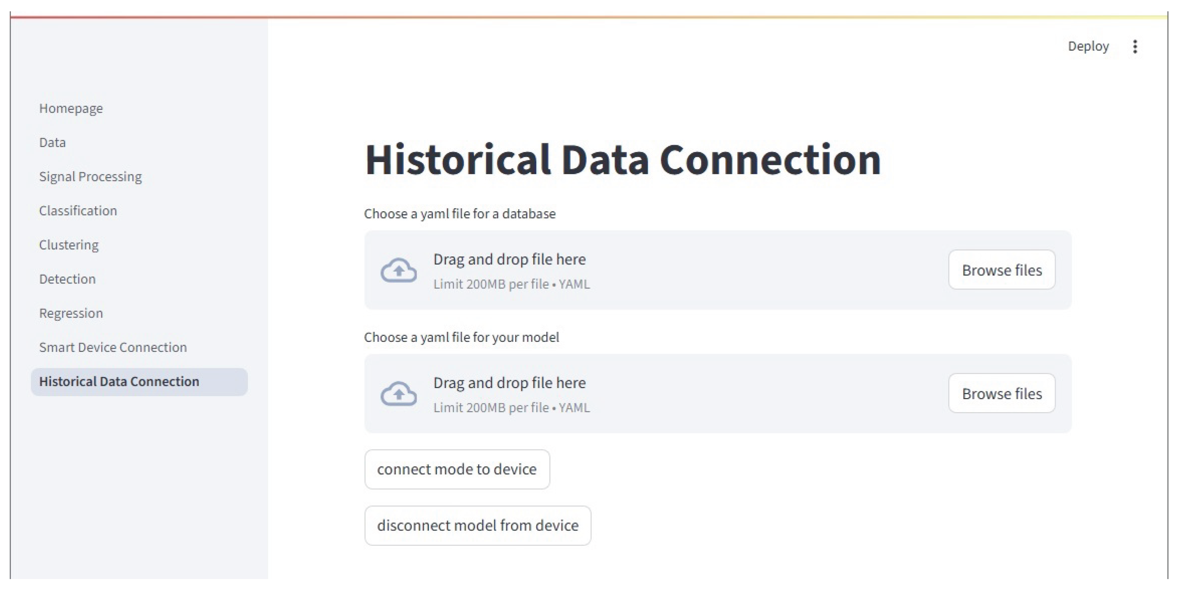
Figure 13.
The Tutorial Page allows users to view the frameworks associated tutorial slides. Here, the classification tutorial title slide is shown.
Figure 13.
The Tutorial Page allows users to view the frameworks associated tutorial slides. Here, the classification tutorial title slide is shown.
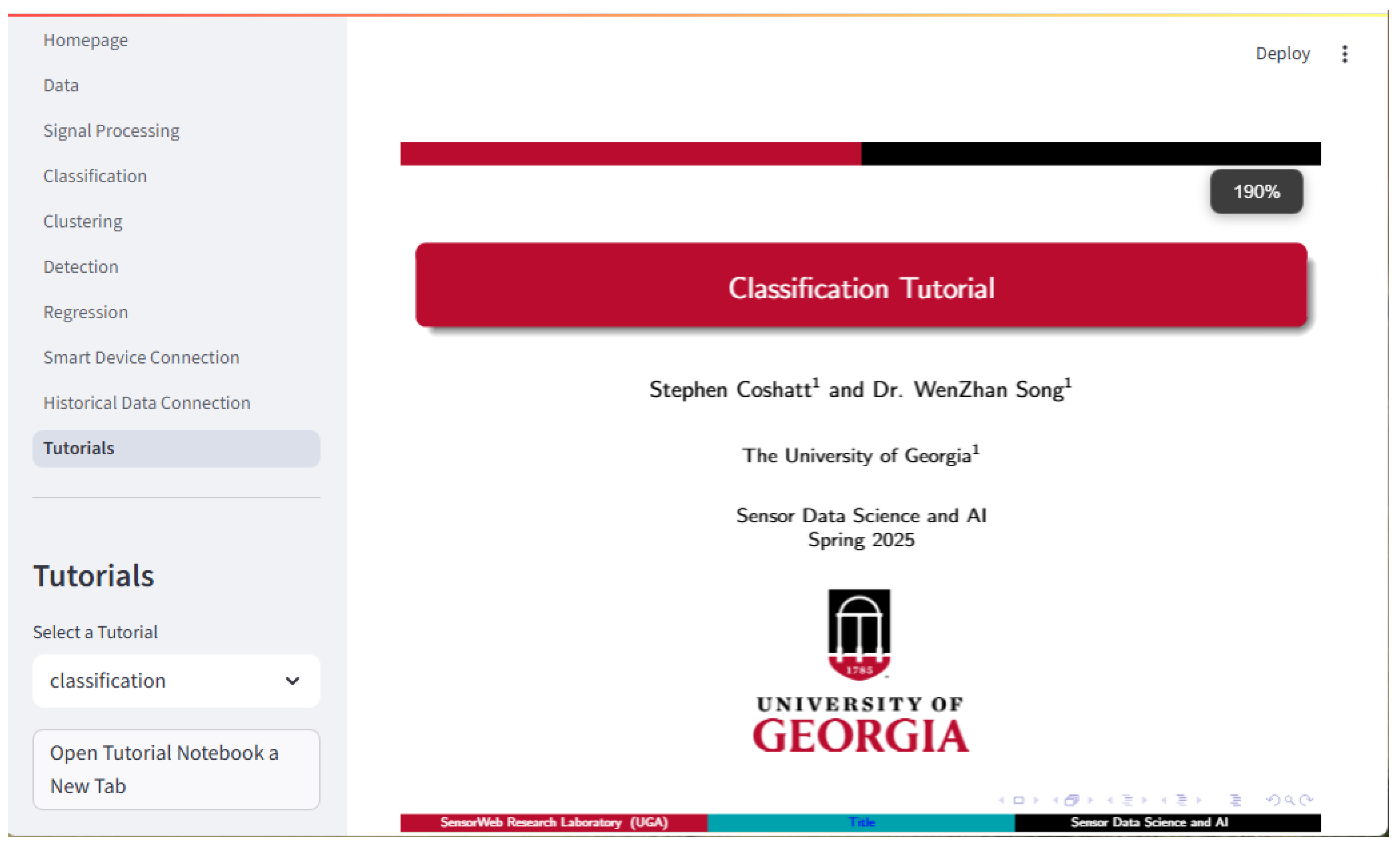
Figure 14.
This image is an example of classification output for the results of an extra trees model. The parameter settings and the metrics as shown in the text. A confusion matrix is also shown.
Figure 14.
This image is an example of classification output for the results of an extra trees model. The parameter settings and the metrics as shown in the text. A confusion matrix is also shown.
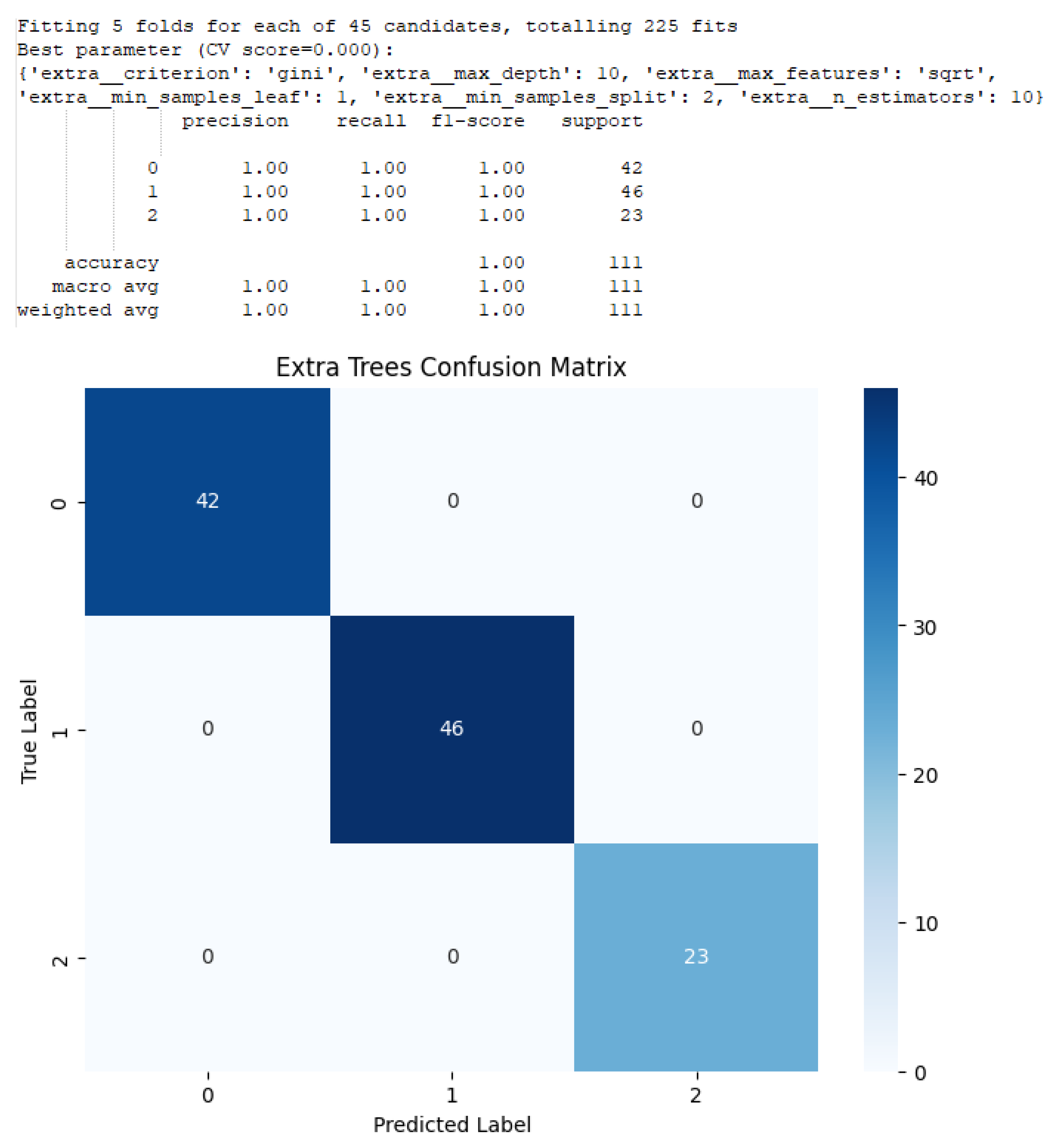

Table 1.
Core Modules.
| Module File Name | Module Information |
|---|---|
| classification.py | Classification, Supervised Anomaly Detection |
| clustering.py | Clustering |
| detection.py | Unsupervised Anomaly Detection |
| dsp.py | Digital Signal Processing |
| regression.py | Regression |
| utils.py | Plotting and other Miscellaneous functions |
a All module files are in the "lib" folder in GitHub.
Table 2.
Tutorials.
| Module | Slides and Notebooks |
|---|---|
| Classification | classification_slides.pdf, classification_tutorial.ipynb |
| Clustering | unsupervised_slides.pdf, unsupervised_tutorial.ipynb |
| DSP | dsp_slides.pdf, dsp_tutorial.ipynb |
| Regression | regression_slides.pdf, regression_tutorial.ipynb |
| Supervised | classification_slides.pdf, classification_tutorial.ipynb |
| Detection | |
| Unsupervised | unsupervised_slides.pdf, unsupervised_tutorial.ipynb |
| Detection |
a All tutorial files are in the "tutorial" folder in GitHub.
Table 3.
The average scores for each model of ten runs are shown in the table below. Each model was score on Accuracy, Precision, Recall, and the F1 Score.
Table 3.
The average scores for each model of ten runs are shown in the table below. Each model was score on Accuracy, Precision, Recall, and the F1 Score.
| Model | Average Scores from 10 runs | |||
|---|---|---|---|---|
| Type | Accuracy | Precision | Recall | F1 Score |
| AdaBoost (trees) | 0.995 | 0.995 | 0.995 | 0.995 |
| Bagging (trees) | 1.00 | 1.00 | 1.00 | 1.00 |
| Decision Tree | 1.00 | 1.00 | 1.00 | 1.00 |
| Extra Trees | 1.00 | 1.00 | 1.00 | 1.00 |
| Gradient Boosting | 1.00 | 1.00 | 1.00 | 1.00 |
| Histogram Grad. Boost | 1.00 | 1.00 | 1.00 | 1.00 |
| KNN | 1.00 | 1.00 | 1.00 | 1.00 |
| Random Forest | 1.00 | 1.00 | 1.00 | 1.00 |
| TS KNN | 1.00 | 1.00 | 1.00 | 1.00 |
Disclaimer/Publisher’s Note: The statements, opinions and data contained in all publications are solely those of the individual author(s) and contributor(s) and not of MDPI and/or the editor(s). MDPI and/or the editor(s) disclaim responsibility for any injury to people or property resulting from any ideas, methods, instructions or products referred to in the content. |
© 2025 by the authors. Licensee MDPI, Basel, Switzerland. This article is an open access article distributed under the terms and conditions of the Creative Commons Attribution (CC BY) license (http://creativecommons.org/licenses/by/4.0/).
Copyright: This open access article is published under a Creative Commons CC BY 4.0 license, which permit the free download, distribution, and reuse, provided that the author and preprint are cited in any reuse.


