
Submitted:
12 September 2025
Posted:
15 September 2025
You are already at the latest version
Abstract
In this paper, we present rigorous asymptotic componentwise perturbation bounds for regular Hermitian indefinite matrix eigendecompositions, obtained by the method of the splitting operators. The asymptotic bounds are derived from the exact nonlinear expressions for the perturbations and make possible to bound each entry of every matrix eigenvector in case of distinct eigenvalues. In contrast to the perturbation analysis of the Schur form of a nonsymmetric matrix, the bounds obtained do not make use of the Kronecker product which reduces significantly the necessary memory and volume of computations. This allows to analyze efficiently the sensitivity of high order problems. The eigenvector perturbation bounds are applied to obtain bounds on the angles between the perturbed and unperturbed one-dimensional invariant subspaces spanned by the corresponding eigenvectors. To reduce the bound conservatism in case of high order problems, we propose to implement probabilistic perturbation bounds based on the Markoff inequality. The analysis is illustrated by two numerical experiments of order 5000.
Keywords:
matrix perturbation analysis
; symmetric matrices
; eigenvectors
; asymptotic bounds
; global bounds
1. Introduction
The eigenvalue perturbation analysis of real symmetric and complex Hermitian matrices is a well established part of matrix analysis which is presented in depth in the fundamental works of Kato [12], Wilkinson [31], Parlett [20], Stewart and Sun [27], Bhatia [4], Stewart [26] and Chatelin [7], the surveys of Sun [29] and Li [14], as well as in numerous papers, see for instance [2,11,16,25,28,30] and the references therein. The perturbation analysis of Hermitian decompositions is usually simpler than the analysis of non-symmetric matrix decompositions. (For a survey on the perturbation theory of non-symmetric matrix decompositions, see [10]). The aim of such an analysis is to find perturbation bounds of the eigenvalues and eigenvectors of Hermitian matrices in the case when these matrices are subject to Hermitian or non-Hermitian perturbations. Depending on the problem solved, such an analysis can be a priori, when we want to predict in advance the changes in the eigendecomposition before the perturbation is applied, or a posteriori, when we attempt to find the errors in eigenvalues and eigenvectors based on the computed perturbed quantities [7]. Here we will be concerned with the first type of analysis, the second one being related to the determination of residual bounds as it is considered by several authors, see Davis and Kahan [8], Parlett [Ch. 11][20], Stewart and Sun [Ch. 5][27], Chatelin [7], and Nakatsukasa [18]. On the other hand, the perturbation analysis can be asymptotic, when we are interested in the effect of vanishing perturbations or global, when we want to find guaranteed bounds in the case of sufficiently large perturbations. We note that in most cases the authors are usually concerned with the eigenvalue perturbations and the eigenvector perturbation analysis is reduced to the sensitivity analysis of the corresponding invariant subspace. In several cases this sensitivity analysis is restricted to bounding the distance between the unperturbed and perturbed subspace [28] or finding the angles between these subspaces [14,26,27,29]. However, in some applications it is necessary to have bounds on the individual elements of specific eigenvector, not only on the sensitivity of the corresponding invariant subspace. This leads to the necessity to perform a componentwise perturbation analysis of the matrix eigensystem.
In this paper we are interested to carry out a componentwise perturbation analysis of indefinite Hermitian matrices that allows to bound each element of every corresponding eigenvector. This analysis is done only for regular eigenvalue problems, i.e., perturbation problems for matrices with distinct eigenvalues. The singular problems, corresponding to multiple eigenvalues, are treated by different techniques, see [6,15]. The regular problems can be solved simply and efficiently by using the method of splitting operators [13] which is already implemented to solve several other matrix perturbation problems. It is important that the bounds on eigenvector elements, obtained by this method, can also be used to obtain a bound on the sensitivity of the invariant subspace spanned by the corresponding eigenvector.
Theoretically, the perturbation analysis of Hermitian decompositions can be done by using some of the methods intended for non-Hermitian problems. This, however, may require much larger memory and volume of computations. For instance, the similar method for perturbation analysis of the Schur form proposed in [21], requires to construct large matrices by implementing the Kronecker product. The method presented in this paper avoids the using of such product which makes possible to analyze much larger problems.
Consider a Hermitian matrix . Using a unitary transformation matrix , the matrix A is reduced to the diagonal form
where are the eigenvalues of A and is the matrix of the corresponding orthonormal eigenvectors. Note that the eigenvalues of a Hermitian matrix are always real. If A is real, then U is orthogonal [9,20]. The diagonal decomposition (1) is also referred to as symmetric Schur decomposition. Further on, without loss of generality, we will assume that the eigenvalues of A are ordered such that .
If the matrix A is subject to a Hermitian perturbation , then instead of the decomposition (1) we have the new diagonal decomposition
where are the perturbed eigenvalues and is the matrix of the perturbed eigenvectors.
The aim of the perturbation analysis is to determine bounds on the eigenvalue perturbations and the corresponding eigenvector perturbations . The perturbation problem for Hermitian matrices eigendecompositions is regular, if and only if the eigenvalues of A are distinct. An additional important problem is to determine the sensitivity of the one-dimensional invariant subspaces spanned by the eigenvectors . According to the Wielandt-Hofmann theorem [9], the eigenvalues of a Hermitian matrix are always well conditioned since their perturbations obey
However, the eigenvectors can be very sensitive to perturbations of A, depending on the separation of the eigenvalues, see for instance [25].
According to the splitting operator method [13], it is possible to derive separately perturbation bounds on and which allows to obtain tighter perturbation bounds on the eigenvector. For this aim, it is appropriate to introduce the matrix
which is unitary equivalent to the unknown matrix . Finding estimates of the entries of this matrix allows to find sharp bounds on the entries of thanks to the orthogonality of the matrix U.
Further on, we shall use the perturbation parameter vector
where the components of x are the entries of the strictly lower triangular part of . Using this vector, it is convenient to find bounds on various quantities related to the perturbation analysis of A.
The paper is organized as follows. In sect. Section 2, we derive asymptotic bounds on the perturbation parameters which are then used in the perturbation analysis of eigenvalues and eigenvectors of a symmetric matrix. The eigenvector perturbation bounds are used to find asymptotic bounds on the perturbations of the invariant subspaces spanned by the eigenvectors. In sect. Section 3, we briefly present some results concerning the determination of realistic probabilistic bounds on the entries of a random matrix using its Frobenius norm. We describe the implementation of such bounds in the derivation of probabilistic perturbation bounds on the eigenvector entries, eigenvalues and invariant subspaces. We illustrate the theoretical results in Sect. Section 4 by presenting two numerical experiments with matrices of order 5000 demonstrating the performance of the derived bounds. Some conclusions are made in sect. Section 5.
All computations in the paper are done with MATLAB® Version 9.9 (R2020b) [17] using IEEE double precision arithmetic on a machine equipped with an 12th Gen Intel(R) Core(TM) i5-1240P CPU running at 1.70 GHz and with 32 GB of RAM. M-files implementing the perturbation bounds described in the paper can be obtained from the authors.
2. Asymptotic Perturbation Bounds
2.1. Asymptotic Bounds for the Perturbation Parameters
Theorem 1.
Let be a Hermitian matrix () with distinct eigenvalues , which is decomposed as , where U is unitary and Λ is diagonal. Assume that the matrix A is perturbed by a Hermitian perturbation , so that
Denote by the transformed perturbation matrix and construct the vector
Then the perturbation parameters
satisfy the equation
where is a diagonal matrix of the form
 with and is a vector containing second order terms in .
Since the matrices U and are unitary, it follows that
and hence
Replacing this expression for into (6), we obtain that
or
The expression (9) can be rewritten as a system of nonlinear algebraic equations for the unknown quantities
in the form (3), where the component of the nonlinear term is equal to
❒
We note that the solution of the system of equations (3) does not require the explicit formation of the matrix M. In particular, the asymptotic bound in the inequality
can be obtained easily by using the expression
Example 1.
Consider the matrix
The eigenvalues of this matrix are
Note the closeness of the last three eigenvalues which prompts that the corresponding eigenvectors can be ill conditioned.
The perturbation matrix is taken as
where is a matrix whose elements are random normal numbers.
For this perturbation problem, the matrix , which determines the perturbation parameter vector x in (3) has a 2-norm equal to , which confirms that the problem is relatively ill conditioned.
The exact perturbation parameters and their asymptotic approximations computed by using (11), are shown to eight decimal digits in Table 1. Note the good coherence between the magnitude of the corresponding elements of both vectors. The differences between the values of and are due to the bounding of the elements of the vector f by the value of and the neglecting of the nonlinear term .
2.2. Asymptotic Componentwise Eigenvector Bounds
Theorem 2.
Under the conditions of Theorem 1, a strict asymptotic bound on the perturbation of each eigenvector of A under a perturbation , is given by
where
and the elements of the vector are determined form
Proof. Consider the auxiliary matrix
introduced above. As already noted, the strictly lower part of this matrix contains elements of the form
which can be substituted by the corresponding elements of the vector x. The elements of the strictly upper part of are of the form
which, according to the unitary condition (7), can be represented as
or
where the term is the conjugate value of the element . Hence the matrix can be represented as
where
and the matrices
contain second order terms in . Note that for definiteness, we have assumed that is chosen so that the diagonal elements of are real and
since the condition (12) does not restrict the imaginary part of .
According to (13), the matrix can be estimated as
where
contains second order terms in the elements of x. Thus, an asymptotic (linear) approximation of the matrix can be determined as
❒
Note that the bounds derived are also valid for real symmetric matrices.
Example 2.
For the same matrix A and perturbation as in Example 1, the absolute values of the exact changes of the entries of the matrix U and their linear estimates, obtained by using (15) are, respectively
and
For all it is fulfilled that .
2.3. Eigenvalue Sensitivity
For the changes in the elements of the perturbed diagonal form one has the following expressions
Hence
Thus, we obtain
where, taking into account equations (5), we have that
According to (7), it is fulfilled that
which gives
The quantity contains second order terms in .
If the perturbation is known, expression (19) allows to obtain bound on using the eigenvector bound (15).
In the asymptotic eigenvalue analysis the higher order terms are neglected and one has
Hence,
which reduces to the well known corollary of the Wielandt-Hoffman theorem [9].
2.4. Sensitivity of One Dimensional Invariant Subspaces
The estimate of the eigenvector perturbation can be used to find an estimate of the one dimensional (simple) invariant subspace, associated with the eigenvector .
Consider the one dimensional invariant subspace . The sensitivity of this subspace is measured by the angle between the perturbed and unperturbed invariant subspace. Since
we have that [5,26]
where
is the orthogonal complement of .
Equation (20) shows that the sensitivity of the one dimensional invariant subspace is connected to the values of the perturbation parameters . Consequently, if bounds on the perturbation parameters are known, it is possible to find the sensitivity estimates of all invariant subspaces. More specifically, we have that
Then we obtain that the angle between the jth perturbed and unperturbed invariant subspace has the following asymptotic estimate
We note that this estimate produces practically the same results as the linear bound derived in [3,28,29].
Example 3.
For the same matrix and perturbation, as in the previous examples, the exact angles between the perturbed and unperturbed one-dimensional invariant subspaces and their linear estimates, are shown in Table 2.
3. Probabilistic Asymptotic Bounds
The numerical experiments with symmetric matrices show that the estimates obtained by using Theorem 2 can become very pessimistic with the increasing of matrix order. For instance, if the matrix is of order 2000, then the ratio between the bound (15) and the actual values of the entries of may become of order which makes the computed bound useless. A further reduction of the perturbation bounds can be achieved by implementing probabilistic perturbation bounds which for large n allow to obtain sufficiently close bounds with a high probability. For this aim we will make use of the probabilistic matrix bounds proposed in [23,24] that are based on the Markoff inequality [19].
Consider briefly the essence of the approach presented in [23]. The aim is to reduce the size of entries of an estimate of the matrix perturbation at the price that some entries of are smaller then the corresponding entries of . We have the following result.
Theorem 3.
Let be an estimate of the random perturbation and be the probability that . If the entries of are chosen as
where
and is a desired probability, then it is fulfilled that
If the number is sufficiently large so that , Theorem 3 allows to decrease the mean value of the bound and hence the magnitude of its entries by the scaling factor , choosing the desired probability less than 1. Note that the probability bound produced by the Markoff inequality is conservative, the actual results usually being much better than the results predicted by the quantity . This is due to the fact that the Markoff inequality is valid for the worst possible distribution of the random variables, but in the given case we do not impose a restriction on the probability distribution of the entries of .
According to Theorem 3, the using of the scaling factor (22) guarantees that the inequality
holds for each i and j with probability no less than .
Using Theorem 3, a probability bound on the perturbation parameters can be determined by the following theorem.
Theorem 4.
If the asymptotic estimate of the perturbation parameter vector x is chosen as
where Ξ is determined according to
then
The inequality (25) shows that the probability estimate of the component can be determined, if in the linear estimate (11) we replace the perturbation norm by the probability estimate , where the scaling factor is taken as shown in (22) for a specified probability .
The probabilistic perturbation bounds on the elements of the vector x allow to find probabilistic bounds on the elements of .
Theorem 5.
An asymptotic bound with probability on the perturbation of each eigenvector of A under a perturbation , is given by
where
and the elements of the vector are determined form
The probabilistic bound on produces the following asymptotic perturbation bounds on the eigenvalues of A:
Finally, we obtain that the angle between the jth perturbed and unperturbed one-dimensional invariant subspace satisfies the probabilistic asymptotic estimate
4. Numerical Experiments
In this section, we present two numerical experiments for determining the perturbation bounds for the eigendecompositions of matrices of order 5000. The matrices are constructed in the form where V is orthogonal and D is a diagonal matrix containing the desired eigenvalues. The perturbation is taken as , where is a matrix whose elements are normal random numbers.
Example 4.
In this examples the eigenvalues of A are taken uniformly between 1 and 5.999 with an increment equal to 0.001, which results in matrix with a 2-norm equal to .
In Figure 1 we show the entries of the exact perturbation and the entries of the asymptotic and probabilistic bounds. The desired lower bound probability is set to and the scaling factor in finding the probabilistic estimates is equal to 1000. In a result, the actual probability is equal to , since the bounds of all entries of exceed the corresponding entries of . As already mentioned, this phenomenon is due to the conservatism of the Markoff inequality. The eigenvalue perturbations along with their asymptotic and probability estimates, are shown in Figure 2. There are no eigenvalues whose probability perturbation bound is smaller than the actual , which gives accuracy instead of the reference value . Due to the equal space between the eigenvalues, in the given case the sensitivity of all invariant subspaces is the same (Figure 3). Clearly, the probabilistic estimates are much closer to the actual perturbations than the linear deterministic bounds.
Example 5.
In this example the eigenvalues of A are taken as and are spread between and 501, the norm of the matrix being equal to . The eigenvalues of A are shown in Figure 4.
In Figure 5, Figure 6 and Figure 7 we show the matrix , the eigenvalue perturbations and the angles between the perturbed and unperturbed invariant subspaces, respectively, as well as their asymptotic and probabilistic bounds for . Due to the decreasing distance between the eigenvalues, the sensitivity of the invariant subspace is increasing with the sequence number i. The actual probabilistic bounds for the eigenvector matrix and for the eigenvalues are again equal to as in the previous example.
Note that in both examples, the linear estimates reflect correctly the changes of the corresponding exact quantities.
5. Conclusions
In this paper, we present strict asymptotic perturbation bounds of the eigenvalues, eigenvectors and invariant subspaces of symmetric and Hermitian matrices. The implementation of the splitting operator method makes possible to unify the analysis with the perturbation analysis of the Schur form [21], the generalized Schur form [32], the singular value decomposition [1] and the QR decomposition of a matrix [22]. Since the deterministic bounds derived can be conservative especially for high-order matrices, we present probabilistic bounds based on the Markoff inequality. The probabilistic bounds are found easily from the asymptotic bounds and allow to decrease significantly the perturbation bounds with a guaranteed probability which is near to 1 in practice. An attractive future of the bounds for symmetric matrices is that these bounds can be determined with low requirements in respect to the necessary memory and volume of computations.
6. Notation
| , | the set of complex numbers; |
| , | the space of complex matrices; |
| , | a matrix with entries ; |
| , | the jth column of A; |
| , | the ith row of an matrix A; |
| , | the jth column of an matrix A; |
| , | the strictly lower triangular part of A; |
| , | the matrix of absolute values of the elements of A; |
| , | the Hermitian transposed of A; |
| , | the zero matrix; |
| , | the unit matrix; |
| , | the perturbation of A; |
| , | the spectral norm of A; |
| , | the Frobenius norm of A; |
| , | equal by definition; |
| ⪯, | relation of partial order. If , then means |
| ; | |
| , | the subspace spanned by the columns of X; |
| , | the orthogonal complement of U, ; |
| ❒, | the end of a proof. |
Funding
This research received no external funding.
Institutional Review Board Statement
Not applicable.
Informed Consent Statement
Not applicable.
Data Availability Statement
The datasets generated during the current study are available from the author upon reasonable request.
Conflicts of Interest
The author declares that the research was conducted in the absence of any commercial or financial relationships that could be construed as a potential conflict of interest.
References
- V. Angelova and P. Petkov, Componentwise perturbation analysis of the Singular Value Decomposition of a matrix, Applied Sciences, 14 (2024), 1417. [CrossRef]
- J. Barlow and I. Slapničar, Optimal perturbation bounds for the Hermitian eigenvalue problem, Lin. Alg. Appl., 309 (2000), pp. 19–43. [CrossRef]
- Z. Bai and J. Demmel and A. Mckenney, On computing condition numbers for the nonsymmetric eigenproblem, ACM Trans. Math. Software, 19 (1993), 202–223. [CrossRef]
- R. Bhatia, Perturbation Bounds for Matrix Eigenvalues, Society of Industrial and Applied Mathematics, Philadelphia, PA, 2007. 8987; -3. [CrossRef]
- A. Björck and G. Golub, Numerical methods for computing angles between linear subspaces, Math. Comp., 27 (1973), pp. 579–594. [CrossRef]
- M. Carlsson, Spectral perturbation theory of Hermitian matrices, in: Bridging Eigenvalue Theory and Practice – Applications in Modern Engineering, B. Carpentieri, ed., IntechOpen, London, 2025. 8363; -9. [CrossRef]
- F. Chatelin, Eigenvalues of Matrices, Society of Industrial and Applied Mathematics, Philadelphia, PA, 2012. ISBN 978-1-611972-45-0. [CrossRef]
- C. Davis and W. M. Kahan, The Rotation of Eigenvectors by a Perturbation. III, SIAM J. Numer. Anal., 7 (1970), pp. 46. [CrossRef]
- G. H. Golub and C. F. Van Loan, Matrix Computations, The Johns Hopkins University Press, Baltimore, MD, fourth ed., 2013. ISBN 978-1-4214-0794-4.
- A. Greenbaum and R.-C. Li and M.L. Overton, First-order perturbation theory for eigenvalues and eigenvectors, SIAM Review, 62 (2020), pp. 463–482. [CrossRef]
- I.C.F. Ipsen, An overview of relative sin(Θ) theorems for invariant subspaces of complex matrices. J. Comp. Appl. Math., 123 (2000), pp. 131–153. [CrossRef]
- T. Kato, Perturbation Theory for Linear Operators, Springer-Verlag, Berlin, second ed., 1995. ISBN 978-0-540-58661-6.
- M. Konstantinov and P. Petkov, Perturbation Methods in Matrix Analysis and Control, NOVA Science Publishers, Inc., New York, 2020. https://novapublishers.com/shop/perturbation-methods-in-matrix-analysis-and-control.
- R. Li, Matrix perturbation theory, in Handbook of Linear Algebra, L. Hogben, ed., Discrete Math. Appl., CRC Press, Boca Raton, FL, second ed., 2014, pp. (21–1)–(21–20).
- <sc>R.-C. Li, Y. R.-C. Li, Y. Nakatsukasa, N. Truhar and W.-g. Wang, Perturbation of multiple eigenvalues of Hermitian matrices, Linear Algebra Appl., 437 (2012), pp. 202–213. [CrossRef]
- R. Mathias, Quadratic residual bounds for the Hermitian eigenvalue problem, SIAM J. Matrix Anal. Appl., 19 (1998), pp. 541–550. [CrossRef]
- The MathWorks, Inc., MATLAB Version 9.9.0.1538559 (R2020b), Natick, MA, 2020. https://www.mathworks.com.
- Y. Nakatsukasa, Sharp error bounds for Ritz vectors and approximate singular vectors, Math. Comput., 89 (2018), pp. 1843–-1866. [CrossRef]
- A. Papoulis, Probability, Random Variables and Stochastic Processes, McGraw Hill, Inc., New York, 3rd edition, 1991. ISBN 0-07-048477-5.
- B.N. Parlett, The Symmetric Eigenvalue Problem, Society of Industrial and Applied Mathematics, Philadelphia, PA, 1998. [CrossRef]
- P. Petkov, Componentwise perturbation analysis of the Schur decomposition of a matrix, SIAM J. Matrix Anal. Appl., 42 (2021), pp. 108–133. [CrossRef]
- P. Petkov, Componentwise perturbation analysis of the QR decomposition of a matrix, Mathematics, 10 (2022). [CrossRef]
- P. Petkov, Probabilistic perturbation bounds of matrix decompositions, Numer. Linear Algebra Appl., 31(2024), pp. 1–40. [CrossRef]
- P. Petkov, Probabilistic perturbation bounds for invariant, deflating and singular subspaces, Axioms, 13(2024), 597. [CrossRef]
- G.W. Stewart, Error and perturbation bounds for subspaces associated with certain eigenvalue problems, SIAM Review, 15 (1973), pp. 727–764. [CrossRef]
- G. Stewart, Matrix Algorithms; Vol. II: Eigensystems, SIAM: Philadelphia, PA, 2001; ISBN 0-89871-503-2. [Google Scholar]
- G. W. Stewart and J.-G. Sun, Matrix Perturbation Theory, Academic Press, New York, 1990. ISBN 978-0126702309.
- J.-g. Sun, Perturbation expansions for invariant subspaces, Linear Algebra Appl., 153 (1991), pp. 85–97. [CrossRef]
- J.-g. Sun, Stability and Accuracy. Perturbation Analysis of Algebraic Eigenproblems. Technical Report, Department of Computing Science, Umeå University, Umeå, Sweden, 1998, pp. 1–210.
- K. Veselić and I. Slapničar, Floating-point perturbations of Hermitian matrices, Linear Algebra Appl., 195 (1993), pp. 81–116. [CrossRef]
- J. Wilkinson, The Algebraic Eigenvalue Problem. Clarendon Press, Oxford, UK, 1965. ISBN 978-0-19-853418-1.
- G. Zhang and H. Li and Y. Wei, Componentwise perturbation analysis for the generalized Schur decomposition, Calcolo, 59 (2022). [CrossRef]
Figure 1.
The entries of the matrix and their asymptotic and probabilistic bounds for Example 4
Figure 2.
The eigenvalue perturbations and their asymptotic and probabilistic bounds for Example 4
Figure 3.
Angles between the perturbed and unperturbed invariant subspaces and their asymptotic and probabilistic bounds for Example 4
Figure 3.
Angles between the perturbed and unperturbed invariant subspaces and their asymptotic and probabilistic bounds for Example 4
Figure 4.
The matrix eigenvalues for Example 5
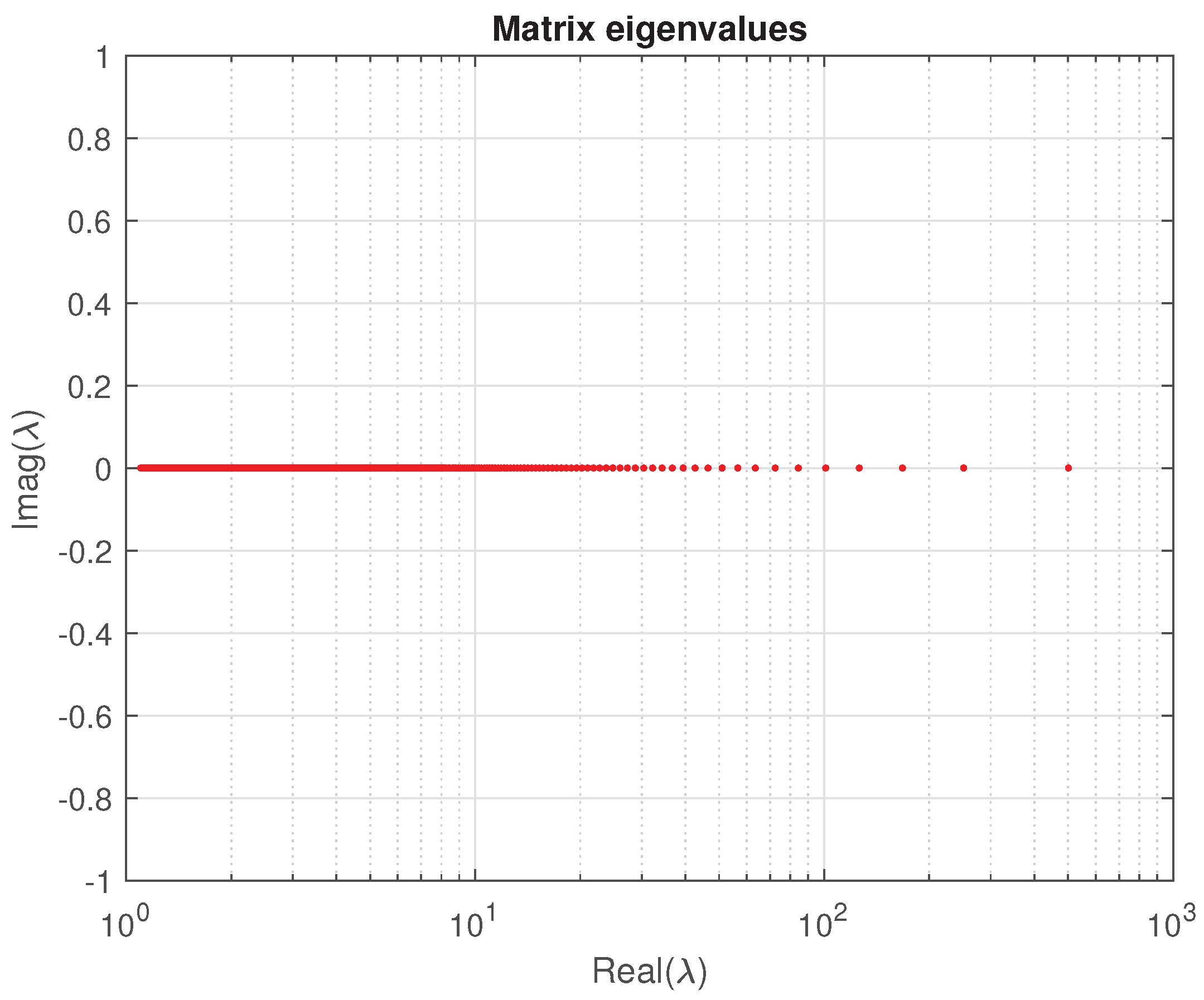
Figure 5.
The entries of the matrix and their asymptotic and probabilistic bounds for Example 5
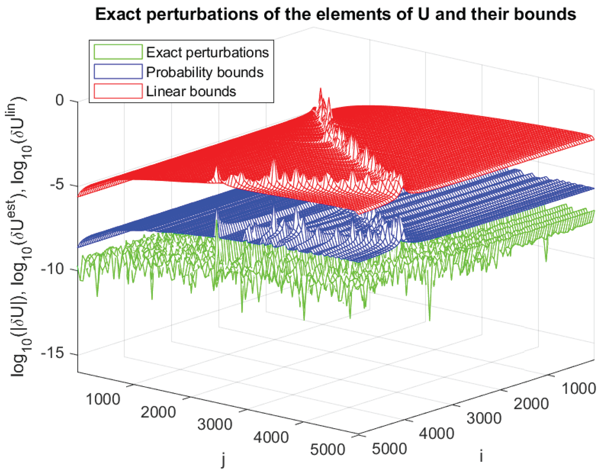
Figure 6.
The eigenvalue perturbations and their asymptotic and probabilistic bounds for Example 5
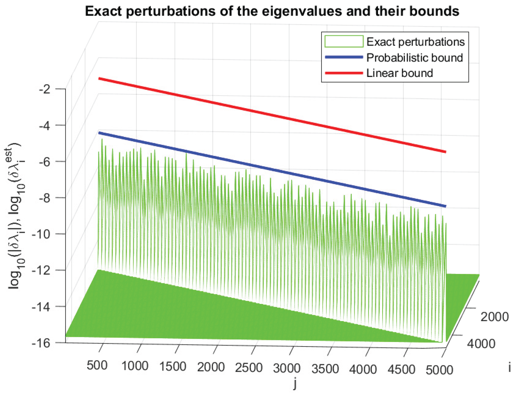
Figure 7.
Angles between the perturbed and unperturbed invariant subspaces and their asymptotic and probabilistic bounds for Example 5
Figure 7.
Angles between the perturbed and unperturbed invariant subspaces and their asymptotic and probabilistic bounds for Example 5
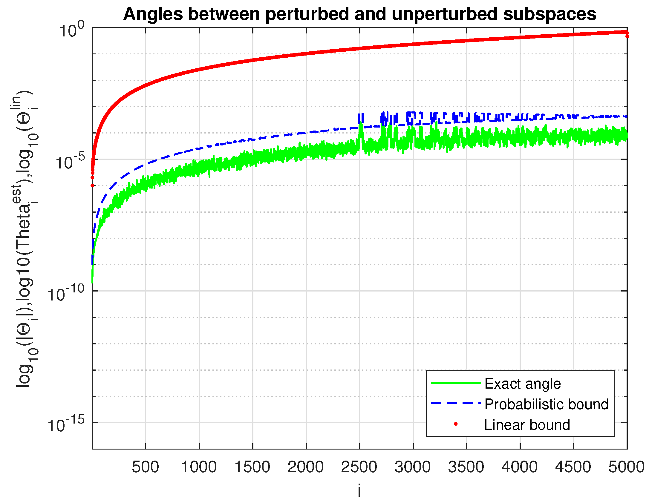

Table 1.
Exact perturbation parameters related to the matrix and their linear estimates for
Table 2.
Exact angles between perturbed and unperturbed invariant subspaces and their linear estimates
Table 2.
Exact angles between perturbed and unperturbed invariant subspaces and their linear estimates
| j | ||
|---|---|---|
| 1 | ||
| 2 | ||
| 3 | ||
| 4 | ||
| 5 |
Disclaimer/Publisher’s Note: The statements, opinions and data contained in all publications are solely those of the individual author(s) and contributor(s) and not of MDPI and/or the editor(s). MDPI and/or the editor(s) disclaim responsibility for any injury to people or property resulting from any ideas, methods, instructions or products referred to in the content. |
© 2025 by the authors. Licensee MDPI, Basel, Switzerland. This article is an open access article distributed under the terms and conditions of the Creative Commons Attribution (CC BY) license (http://creativecommons.org/licenses/by/4.0/).
Copyright: This open access article is published under a Creative Commons CC BY 4.0 license, which permit the free download, distribution, and reuse, provided that the author and preprint are cited in any reuse.


