
Submitted:
13 November 2023
Posted:
14 November 2023
You are already at the latest version
Abstract
A rigorous perturbation analysis of the singular value decomposition
of a real matrix of full column rank is presented. It is shown that the
SVD perturbation problem is well posed only in case of distinct singular values.
The analysis involves the solution of coupled systems of linear equations and
produces asymptotic (local) componentwise perturbation bounds of the entries of
the orthogonal matrices participating in the decomposition of the given matrix
and of its singular values. Local bounds are derived for the
sensitivity of the singular subspaces measured by the angles between the
unperturbed and perturbed subspaces. An iterative scheme is described to find
global bounds on the respective perturbations. The analysis implements the same
methodology used previously to determine componentwise perturbation bounds of
the Schur form and the QR decomposition of a matrix.
Keywords:
singular value decomposition (SVD)
; singular values
; singular subspaces
; perturbation analysis
; componentwise perturbation bounds
MSC: 15A18; 65F25; 47A55; 47H14
1. Introduction
As it is known [5, Ch. 2], [13, Ch. 1], [4, Ch, 2], each real matrix A can be represented by the singular value decomposition (SVD) in the factorized form
where the matrix U and the matrix V are orthogonal and the matrix is diagonal:
The numbers are called singular values of the matrix A. The columns of
are called left singular vectors and the columns of
are the right singular vectors. The subspaces spanned by sets of left and right singular vectors are called left and right singular subspaces, respectively.
The usual assumption is that by an appropriate ordering of the columns and , the singular values appear in the order
but in this paper we will not impose such a requirement.
The SVD has a lot of properties which make it an invaluable tool in matrix analysis and matrix computations, see the references cited above. Among them is the fact that the rank of A is equal to the number of its nonzero singular values as well as the equality . The singular value decomposition has a long and interesting history which is described in [12].
In this paper we are interested in the case when the matrix A is subject to an additive perturbation . In such a case there exists another pair of orthogonal matrices and and a diagonal matrix , such that
The perturbation analysis of the singular value decomposition consists in determining the changes of the quantities related to the elements of the decomposition due to the perturbation . This includes determining bounds on the changes of the entries of the orthogonal matrices which reduce the original matrix to diagonal form and bounds on the perturbations of the singular values. Hence, the aim of the analysis is to find bounds on the sizes of , and as functions of the size of . According to the Weyl’s theorem [13, Ch. 1], we have that
which shows that the singular values are perturbed by no more than the 2-norm of the perturbation of A, i.e., the singular values are always well conditioned. The SVD perturbation analysis is well defined if the matrix A is of full column rank n, i.e. since otherwwise the corresponding left singular vector is undetermined.
The size of the perturbations , , and is usually measured by using some of the matrix norms which leads to the so called normwise perturbation analysis. In several cases we are interested in the size of the perturbations of the individual entries of , and , so that it is necessary to implement a componentwise perturbation analysis. This analysis has an advantage in the cases when the individual components of and differ very much in magnitude and the normwise estimates do not produce tight bounds on the perturbations.
The first results in the perturbation analysis of the singular value decomposition are obtained by Wedin [16] and Stewart [10], who developed estimates of the sensitivity of pairs of singular subspaces, see also [14, Ch. V]. Other results concerning the sensitivity of the SVD can be found in [3] and [15]. Several results concerning the sensitivity of the SVD are summarized in [6] and a survey on the perturbation theory of the singular value decomposition can be found in [11]. It should be pointed out that a componentwise perturbation analysis of the SVD apart from several results about the sensitivity of the singular values, is not available up to the moment.
In this paper we present a rigorous perturbation analysis of the orthogonal matrices, singular subspaces and singular values of a real matrix of full column rank. It is shown that the SVD perturbation problem is well posed only in case of distinct (simple) singular values. The analysis produces asymptotic (local) componentwise perturbation bounds of the entries of the orthogonal matrices U and V and of the singular values of the given matrix. Local bounds are derived for the sensitivity of a pair of singular subspaces measured by the angles between the unperturbed and perturbed subspaces. An iterative scheme is described to find global bounds on the respective perturbations and results of numerical experiments are presented. The analysis performed in the paper implements the same methodology as the one used previously in [8,9] to determine componentwise perturbation bounds of the Schur form and QR decomposition of a matrix. However, the SVD perturbation analysis has some distinctive features which makes it a self-dependent problem.
The paper is organized as follows. In Section 2 we derive the basic nonlinear algebraic equations used to perform the perturbation analysis of the SVD. After introducing in Section 3 the perturbation parameters that determine the perturbations of the matrices U and V, we derive a system of coupled equations for these parameters in Section 4. The solution of the equations for the first-order terms of the perturbation parameters allows to find asymptotic bounds on the parameters in Section 5, on the singular values in Section 6 and on the perturbations in the matrices U and V in Section 7. Using the bounds on the perturbation parameters, in Section 8 we derive bounds on the sensitivity of singular subspaces. In Section 9, we develop an iterative scheme for finding global bounds on the perturbations and in Section 10 we present the results of two higher order examples illustrating the proposed analysis. Some conclusions are drawn in Section 11.
2. Basic Equations
Equation (4) is rewritten as
where and the matrix
contains only higher-order terms in the elements of , and .
Let the matrices U and be divided as and , respectively. Since the matrix A can be represented as , the matrix is not well determined but should satisfy the orthogonality condition . The perturbation is also undefined, so that we can bound only the perturbations of the entries in the first n columns of U, i.e., the entries of . Further on, we shall use (5) to determine componentwise bounds on , and .
3. Perturbation Parameters and Perturbed Orthogonal Matrices
In the perturbation analysis of the SVD, it is convenient to find first componentwise bounds on the entries of the matrices and , which are related to the corresponding perturbations and by orthogonal transformations. The implementation of the matrices and allows to find bounds on
and
using orthogonal transformations without increasing the norms of and . This helps to determine bounds on and which are as tight as possible.
Consider first the matrix
Further on, we shall use the vector of the subdiagonal entries of the matrix ,
where
As it will become clear latter on, together with the orthogonality condition
the vector x contains the whole information which is necessary to find the perturbation . This vector may be expressed as
or, equivalently,
where
is a matrix that “pulls out”the p elements of x from the elements of (we consider as a non-existing matrix).
We have that
In a similar way, we introduce the vector of the subdiagonal entries of the matrix (note that V is a square matrix),
where . It is fulfilled that
or, equivalently,
where
In this case
Further on the quantities and will be referred to as perturbation parameters since they determine the perturbations and , as well as the sensitivity of the singular values and singular subspaces.
Consider the matrix
Using the vector x of the perturbation parameters, this matrix is written in the form
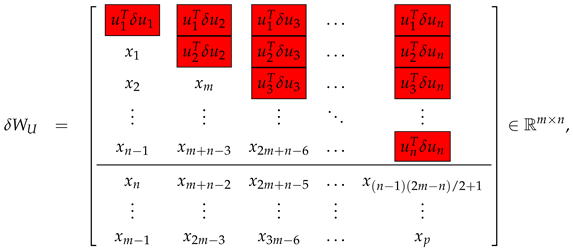 where the diagonal and super-diagonal entries that are not determined up to the moment, are highlighted in red boxes.
Consider how to determine the diagonal elements of the matrix ,
by the elements of x. Since , according to (9), we have that
or
The above expression shows that is always negative and is of second order of magnitude in .
Let us determine now the entries of the super-diagonal part of . Since , it follows that
and
According to the orthogonality condition (9), the entries of the strictly upper triangular part of can be represented as
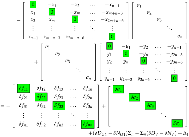
Thus, the matrix can be represented as the sum
where the matrix
has entries depending only on the perturbation parameters x,
and the matrix
contains second order terms in .
Similarly, for the matrix
like to the case of , it is possible to show that
where
has elements depending only on the perturbation parameters y,
and the matrix
contains second order terms in . The diagonal entries of are determined as in the case of the matrix .
4. Equations for the Perturbation Parameters
The elements of the perturbation parameter vectors x and y can be determined from equation (5). For this aim it is appropriate to transform this equation as follows. Taking into account that and , the equation is represented as
where
According to (8), we have that
Substituting in (12) the term by the sum in the right hand side of (13), we obtain
where
contains higher order terms in the entries of , and .
Replacing the matrices and by and , respectively, (14) is rewritten as
or
Note that the matrices and contain only higher order terms in the entries of and .
The entries of the matrices and can be substituted by the corresponding elements and of the vectors x and y as shown in the previous section. This leads to the representation of equation (16) as two matrix equations in respect to two groups of the entries of x,
 and
where
We note that the estimation of requires to know an estimate of which is undetermined.
and
where
We note that the estimation of requires to know an estimate of which is undetermined.
Equations (17) and (18) are the basic equation of the SVD perturbation analysis. They can be used to obtain asymptotic as well as global perturbation bounds on the elements of the vectors x and y.
Let us introduce the vectors
where
The vector contains the elements of the unknown vector x participating in (17), while contains the elements of x participating in (18). It is easy to prove that
Taking into account that
the strictly lower part of (17) can be represented columnwise as the system of linear equations in respect to the unknown vectors and y,
where
and
It should be noted that the operators and used in (21), (24), take only the entries of the strict lower and strict upper part, respectively, of the corresponding matrix which are placed by the operator column by column excluding the zeros above or under the diagonal, respectively. For instance, if the elements of the vectors f and g satisfy
5. Asymptotic Bounds of the Perturbation Parameters
Equations (21) and (24) can be used to determine asymptotic approximations of the vectors and y. The exact solution of these equations satisfies
where taking into account that and commute, we have that
Exploiting these expressions, it is possible to show that
Let us consider the conditions for existence of a solution of equations (21), (24). These equations have an unique solution for and y, if and only if the matrix
is nonsingular, or equivalently, the matrices , and are nonsingular. The matrices and are nonsingular, since the matrix A has nonzero singular values. In turn, a condition for nonsingularity of the matrix can be found taking into account the structure of the matrices and shown above. Clearly, the denominators of the first diagonal entries of and will be different from zero, if is distinct from . Similarly, the denominators of the next group of diagonal entries will be different from zero if is distinct from and so on. Finally, should be different from . Thus we come to the conclusion that the matrices and will exist and the equations (21), (24) will have an unique solution, if and only if the singular values of A are distinct. This conclusion should not come to surprise, since U is the matrix of the transformation of to Schur (diagonal) form and V is the matrix of the transformation of to diagonal form . On the other hand, the perturbation problem for the Schur form is well posed only when the matrix eigenvalues (the diagonal elements of or ) are distinct.
Neglecting the higher order terms in (26), (27) and approximating each element of f and g by the perturbation norm , we obtain the linear estimates
where
Clearly, if the matrices have large diagonal elements, then the estimates of the perturbation parameters will be large. Using the expressions for and , we may show that
Note that the norms of and can be considered as condition numbers of the vectors and y with respect to the changes of .
An asymptotic estimate of the vector is obtained neglecting the higher order term and approximating its elements according to (25) as
Equation (30) shows that a group of n elements of will be large, if the singular value participating in the corresponding column of Z is small. The presence of large elements in the vector x leads to large entries in and consequently in the estimate of . This observation is in accordance with the well known fact that the sensitivity of a singular subspace is inversely proportional to the smallest singular value associated with this subspace.
As a result of solving the linear systems (28) - (30), we obtain an asymptotic approximation of the vector x as
Example 1.
Consider the matrix
and assume that it is perturbed by
where c is a varying parameter. (For convenience, the entries of the matrix are taken as integers.)
The singular value decompositions of the matrices A and are computed by the functionsvdof MATLAB®[7]. The singular values of A are
In the given case the matrices and in equations (22), (23), are
and the matrices participating in (26), (27) are
The matrix
which determines the solution for and y, has a condition number equal to . The exact parameters and their linear approximates computed by using (28) and (30), are shown to eight decimal digits for two perturbation sizes in Table 1 (the elements obtained from the equations (30) are highlighted in red boxes). The differences between the values of and are due to the bounding of the elements of the vectors f and g by the value of and taking the terms in (28) - (30) with positive signs. Both approximations are necessary to ensure that for arbitrary small size perturbation.
Similarly, in Table 2 we show for the same perturbations of A the exact perturbation parameters and their linear approximations obtained from (29).
6. Bounding the Perturbations of the Singular Values
Equation (17) can also be used to determine linear and nonlinear estimates of the perturbations of the singular values. Considering the diagonal elements of this equation (highlighted in green boxes) and taking into account that , we obtain
or
where denotes the ith diagonal element of . Neglecting the higher order terms, we determine the componentwise asymptotic estimate
Bounding each diagonal element by , we find the normwise estimate of ,
which is in accordance with the Weyl’s theorem (see (3)).
From (32) we also have that
7. Asymptotic Bounds on the Perturbations of and V
Having componentwise estimates for the elements of x and y, it is possible to find bounds on the entries of the matrices and . An asymptotic bound on the absolute value of the matrix is given by
From (6), a linear approximation of the matrix is determined as
The matrix gives bounds on the perturbations of the individual elements of the orthogonal transformation matrix U.
In a similar way we have that the linear approximation of the matrix is given by
From (7) we obtain that
Hence, the entries of the matrix give asymptotic estimates of the perturbations of the entries of V.
For the matrix A of Example 1, we obtain that the absolute values of the exact changes of the entries of the matrix for the perturbation satisfy
and their asymptotic componentwise estimates found by using (34), are
It is seen that the magnitude of the entries of and reflect correctly the magnitude of the corresponding entries of and , respectively. Note that the perturbations of the columns of U and V tend to increase with increasing of the column number.
8. Sensitivity of Singular Subspaces
The sensitivity of a left
or right
singular subspace of dimension r is measured by the angles between the corresponding unperturbed and perturbed subspaces [14, Ch. V].
Let the unperturbed left singular subspace corresponding to the first r singular values is denoted by and its perturbed counterpart as and let and be the orthonormal bases for and , respectively. Then the maximum angle between and is determined from
The expression (36) has the disadvantage that if is small, then and the angle is not well determined. To avoid this difficulty, instead of
it is preferable to work with . It is possible to show that [2]
where is the orthogonal complement of , . Since
we have that
Equation (38) shows that the sensitivity of the left singular subspace is connected to the values of the perturbation parameters . In particular, for the sensitivity of the first column of U (the left singular vector, corresponding to ) is determined as
for one has
and so on, see Figure 1, where the matrices for different values of r are highlighted in boxes and (*) denotes entries which are not used.
In a similar way, utilizing the matrix , it is possible to find the sine of the maximum angle between the perturbed and unperturbed right singular subspace ,
(see Figure 2). Hence, if the perturbation parameters are determined, it is possible to find at once sensitivity estimates for the nested singular subspaces
and
Specifically, as
we have that the exact maximum angle between the perturbed and unperturbed left singular subspace of dimension r is given by
Similarly, the maximum angle between the perturbed and unperturbed right singular subspace of dimension r is
To find an asymptotic estimate of , in the expression for the matrix the elements are replaced by their linear approximations (31). Let
Then the following asymptotic estimate holds,
In particular, for the sensitivity of the range of A we obtain that
Similarly, for the angles between the unperturbed and perturbed right singular subspaces we obtain the linear estimates
We note that the use of separate x and y parameters decouples the SVD perturbation problem and makes it possible to determine the sensitivity estimates of the left and right singular subspaces independently. This is important in cases when the left or right subspace in a pair of singular subspaces is much more sensitive than its counterpart.
Consider the same perturbed matrix A as in Example 1. Computing the matrices and , it is possible to estimate at once the sensitivity of all four pairs of singular subspaces of dimensions corresponding to the chosen ordering of the singular values. In Table 4 we show the actual values of the left and right singular subspaces sensitivity and the computed asymptotic estimates (41) of this sensitivity. To determine the sensitivity of other singular subspaces, it is necessary to reorder the singular values in the initial decomposition so that the desired subspace appears in the set of nested singular subspaces. Also, the computations related to the determining of the linear estimates should be done again.
9. Global Perturbation Bounds
Since analytical expressions for the global perturbation bounds of the singular value decompositions are not known up to this moment, we present an iterative procedure for finding estimates of these bounds based on the asymptotic analysis presented above. This procedure is similar to the corresponding iterative schemes proposed in [8,9], but is more complicated since the determining of bounds on the parameter vectors x and y must be done simultaneously due to fact that the equations for these parameters are coupled.
9.1. Perturbation Bounds of the Entries of
The main difficulty in determining global bounds of x and y is to find an appropriate approximation of the high order term in (18). As is seen from (20), the determining of such estimate requires to know the perturbation which is not well determined since it contains the columns of the matrix . This perturbation satisfies the equations
which follow from the orthogonality of the matrix
An estimate of can be found based on a suitable approximation of
As shown in [9], a first order approximation of the matrix X can be determined using the estimates
where , and for sufficiently small perturbation the matrix is nonsingular. (Note that is already estimated.) Thus, we have that
9.2. Iterative Procedure for Finding Global Bounds of x and y
Global componentwise perturbation bounds of the matrices U and V can be found using nonlinear estimates of the matrices and , determined by (10) and (11), respectively. Such estimates are found correcting the linear estimates of the perturbation parameters and on each iteration step in a way similar to the one presented in [8] and [9].
Consider the case of estimating the matrix . It is convenient to substitute the terms containing the perturbations in (10) by the quantities
which have the same magnitude as . Since
the absolute value of the matrix (10) can be bounded as
where
Since the unknown column estimates participate in both sides of (48), it is possible to obtain them as follows. The first column of is determined from
where , are the first columns of , , respectively. Then the next column estimates can be determined recursively from
which is equivalent to solving the linear system
where
and is the jth column of . The matrix is upper triangular with unit diagonal and if have small norms, then the matrix is diagonally dominant. Hence, it is very well conditioned with condition number close to 1.
As a result we obtain that
which produces the jth column of .
A similar recursive procedure can be used to determine the quantities . In this case for each j it is necessary to solve the nth order linear system
The estimates of and thus obtained, are used to bound the absolute values of the nonlinear elements and given in (19) and (20), respectively. Utilizing the approximation of , it is possible to find an approximation of the matrix as
where ,
and are given by (45), (46). Then the elements of , are bounded according to (19) and (20) as
Utilizing (26) and (27), the nonlinear corrections of the vectors and y can be determined from
where is estimated by using the corresponding expression (48) and - by a similar expression.
The nonlinear correction of is found from
and the total correction vector is determined from
Now, the nonlinear estimates of the vectors x and y are found from
In this way we obtain an iterative scheme for finding simultaneously nonlinear estimates of the coupled perturbation parameter vectors x and y involving the equations (48) - (51), (52) - (57). In the numerical experiments presented below, the initial conditions are chosen as and , where is the MATLAB®function eps, . The stopping criteria for x- and y-iterations are taken as
where . The scheme converges for perturbations of restricted size. It is possible that y converges while x does not converge.
The nonlinear estimate of the higher term can be used to obtain nonlinear corrections of the singular value perturbations. Based on (32), a nonlinear correction of each singular value can be determined as
so that the corresponding singular value perturbation is estimated as
Note that is known only when the entries of the perturbation are known and usually this is not fulfilled in practice. Nevertheless, the nonlinear correction (58) can be useful in estimating the sensitivity of a given singular value.
In Table 5, we present the number of iterations necessary to find the global bound for the problem considered in Example 1 with perturbations . In the last two columns of the table we give the norm of the exact higher order term and its approximation computed according to (50), (51) (the approximation is given for the last iteration). In particular, for the perturbation , the exact higher order term , found using (19) and (20), is
Implementing the described iterative procedure, after 10 iterations we obtain the nonlinear bound
computed according to (50) and (51) on the base of the nonlinear bound .
The global bounds and , found for different perturbations along with the values of and , are shown in Table 6. The results confirm that the global estimates of x and y are close to the corresponding asymptotic estimates.
In Figure 2 and Figure 3 we show the convergence of the relative errors
and
respectively, at step s of the iterative process for different perturbations . For the given example the iteration behaviours of x and y are close.
As it is seen from the figures, with the increasing of the perturbation size the convergence worsens and for the iteration diverges. This demonstrates the restricted usefulness of the nonlinear estimates which are valid only for limited perturbation magnitudes.
In Table 7 we give normwise perturbation bounds of the singular values along with the actual singular value perturbations and their global bounds found for two perturbations of A under the assumption that the linear bounds of all singular values are known. As it can be seen from the table, the nonlinear estimates of the singular values are very tight.
9.3. Global Perturbation Bounds of and
Having nonlinear bounds of x, y, and , we may find nonlinear bounds on the perturbations of the entries of and V according to the relationships
For the perturbations of the orthogonal matrices of Example 1 we obtain the nonlinear componentwise bounds
and
These bounds are close to the obtained in sect. Section 7 linear estimates and , respectively.
Based on (39), (40), global estimates of the maximum angles between the unperturbed and perturbed singular subspaces of dimension r can be obtained using the nonlinear bounds and of the matrices and , respectively. For the pair of left and right singular subspaces we obtain that
In Table 8 we give the exact angles between the perturbed and unperturbed left and singular subspaces of different dimensions and their nonlinear bounds computed using (61) and (62) for the matrix A from Example 1 and two perturbations . The comparison with the corresponding linear bounds given in Table 4 shows that the two types of bounds produce close results. As in the estimation of the other elements of the singular value decomposition, the global perturbation bounds are slightly larger than the corresponding asymptotic estimates but give guaranteed bounds on the changes of the respective elements although for limited size of .
10. Two Higher Order Examples
In this section, we present the result of two numerical experiments with higher order matrices to illustrate the properties of the asymptotic and global estimates obtained in the paper.
Example 2.
Consider a matrix A, taken as
where , the matrices and are constructed as proposed in [1],
and the orthogonal and symmetric matrices are Householder reflections. The condition numbers of and with respect to the inversion are controlled by the variables σ and τ and are equal to and , respectively. In the given case, , and . The minimum singular value of the matrix A is . The perturbation of A is taken as , where c is a negative number and is a matrix with random entries generated by the MATLAB®function rand
.
In Figure 5, Figure 6, Figure 7, Figure 8, Figure 9 and Figure 10 we show several results related to the perturbations of the singular value decomposition of A for 30 values of c between and . As particular examples, in Figure 5 we display the perturbations of the entry , which is an element of the matrix and in Figure 6 - the perturbations of the entry , both as functions of . The componentwise linear bound reflect correctly the behavior of the actual perturbations and are valid for wide changes of the perturbation size. Note that this holds for all elements of U and V. The global (nonlinear) bounds practically coincide with the linear bounds but do not exist for perturbations whose size is larger than .
singular subspaces of dimension 15. Again, the linear bounds on the angles and are valid for perturbation magnitudes from to and this also holds for singular subspaces of other dimensions.
In Figure 9 and Figure 10 we show the perturbations of the singular values and their nonlinear bounds for perturbations with and . While in the first case the nonlinear bound coincides with the actual change of the singular values, in the second case the bound becomes significantly greater than the actual change due to the overestimating of the higher order term .
Example 3.
Consider a matrix A, constructed as in the previous example for and . The perturbation of A is taken as , where is a matrix with random entries.
In Figure 11 and Figure 12 we show the entries of the matrices and , respectively, along with the corresponding componentwise estimates and . The absolute values of the exact changes in all 100 singular values along with the bounds and are shown in Figure 13. The nonlinear bounds of and are found only for 7 iterations and are visually indistinguishable from the corresponding linear bounds.
11. Conclusions
The SVD perturbation analysis presented in this paper makes possible to determine componentwise perturbation bounds of the orthogonal matrices, singular values and singular subspaces of a full rank matrix. The analysis performed has some peculiarities which make it a challenging problem. On one hand, the SVD analysis is simpler than some other problems, like the QR decomposition perturbation problem. This is due to the diagonal form of the decomposed matrix which, among the other, allows to solve easily the equations for the perturbation parameters avoiding the use of the Kronecker product. On the other hand, the presence of two matrices in the decomposition requires the introduction of two different parameter vectors which are mutually dependent due to the relationship between the perturbations of the two orthogonal matrices. This makes necessary to solve a coupled system of equations about the parameter vectors which complicates the analysis.
The analysis presented in the paper can be extended with minor complications to the case of complex matrices.
Funding
This research received no external funding.
Institutional Review Board Statement
Not applicable
Informed Consent Statement
Not applicable
Data Availability Statement
The datasets generated during the current study are available from the authors on reasonable request.
Conflicts of Interest
The authors declares no conflict of interest.
Abbreviations
| Notation | |
| , | the set of real numbers; |
| , | the space of real matrices (); |
| , | the range of A; |
| , | the subspace spanned by the vectors ; |
| , | the orthogonal complement of the subspace ; |
| , | the matrix of absolute values of the elements of A; |
| , | the transposed of A; |
| , | the inverse of A; |
| , | the jth column of A; |
| , | the ith row of matrix A; |
| , | the part of matrix A from row to and from column to ; |
| , | perturbation of A; |
| , | a quantity of second order of magnitude with respect to ; |
| , | the zero matrix; |
| , | the unit matrix; |
| , | the jth column of ; |
| , | the ith singular value of A; |
| , | the minimum and maximum singular values of A, respectively; |
| ⪯, | relation of partial order. If , then means ; |
| , | the strictly lower triangular part of ; |
| , | the strictly upper triangular part of ; |
| , | the vec mapping of . If A is partitioned columnwise as |
| , then , | |
| , | the Euclidean norm of ; |
| , | the spectral norm of A; |
| , | the maximum angle between subspaces and . |
References
- C. Bavely and G. Stewart, An algorithm for computing reducing subspaces by block diagonalization, SIAM J. Numer. Anal., 16 (1979), pp. 359–367. [CrossRef]
- A. Björck and G. Golub, Numerical methods for computing angles between linear subspaces, Math. Comp., 27 (1973), pp. 579–594. [CrossRef]
- J. g. Sun, Perturbation analysis of singular subspaces and deflating subspaces, Numer. Math., 73 (1996), pp. 235–263. [CrossRef]
- G. H. Golub and C. F. Van Loan, Matrix Computations, The Johns Hopkins University Press, Baltimore, MD, fourth ed., 2013. ISBN 978-1-4214-0794-4.
- R. Horn and C. Johnson, Matrix Analysis, Cambridge University Press, Cambridge, UK, second ed., 2013. ISBN 978-0-521-83940-2.
- R. Li, Matrix perturbation theory, in Handbook of Linear Algebra, L. Hogben, ed., Discrete Math. Appl., CRC Press, Boca Raton, FL, second ed., 2014, pp. (21–1)–(21–20).
- The MathWorks, Inc., MATLAB Version 9.9.0.1538559 (R2020b), Natick, MA, 2020, http://www.mathworks.com.
- P. Petkov, Componentwise perturbation analysis of the Schur decomposition of a matrix, SIAM J. Matrix Anal. Appl., 42 (2021), pp. 108–133. [CrossRef]
- P. Petkov, Componentwise perturbation analysis of the QR decomposition of a matrix, Mathematics, 10 (2022). [CrossRef]
- G. Stewart, Error and perturbation bounds for subspaces associated with certain eigenvalue problems, SIAM Rev., 15 (1973), pp. 727–764. [CrossRef]
- G. Stewart, Perturbation theory for the singular value decomposition. Technical Report CS-TR 2539, University of Maryland, College Park, MD, 1990.
- G. Stewart, On the early history of the singular value decomposition, SIAM Rev., 35 (1993), pp. 551–566. [CrossRef]
- G. Stewart, Matrix Algorithms, vol. I: Basic Decompositions, SIAM, Philadelphia, PA, 1998. ISBN 0-89871-414-1.
- G. Stewart and J.-G. Sun, Matrix Perturbation Theory, Academic Press, New York, 1990. ISBN 978-0126702309.
- R. Vaccaro, A second-order perturbation expansions for the SVD, SIAM J. Matrix Anal. Appl., 15 (1994), pp. 661–671. [CrossRef]
- P.-A. Wedin, Perturbation bounds in connection with singular value decomposition, BIT Numerical Mathematics, 12 (1972), pp. 99–111. [CrossRef]
Figure 1.
Sensitivity estimations of the left singular subspaces.
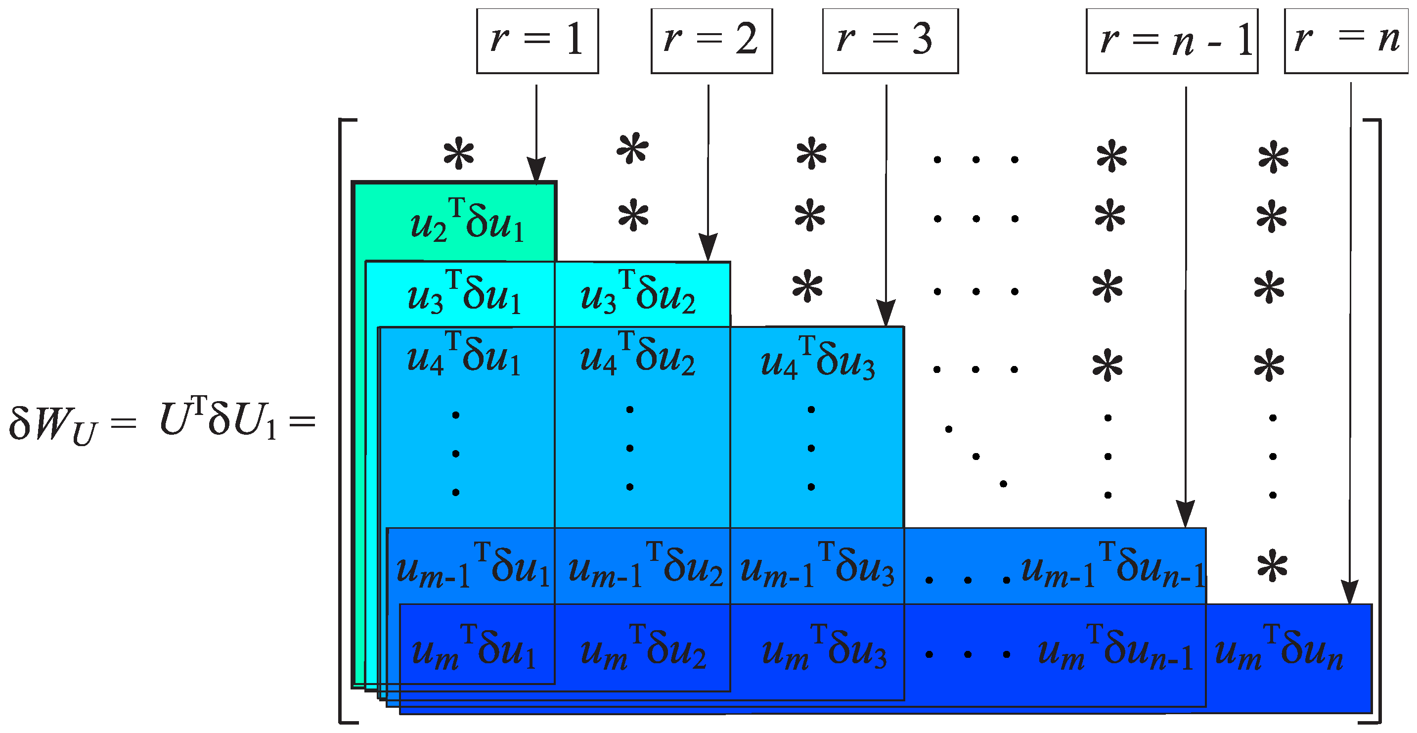
Figure 2.
Sensitivity estimations of the right singular subspaces.
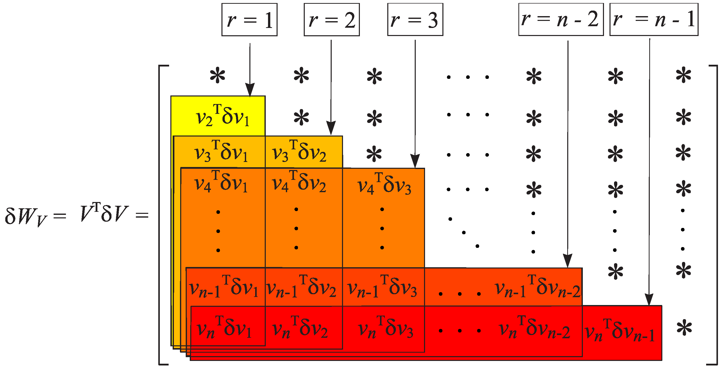
Figure 3.
Iterations for finding the global bounds of x.
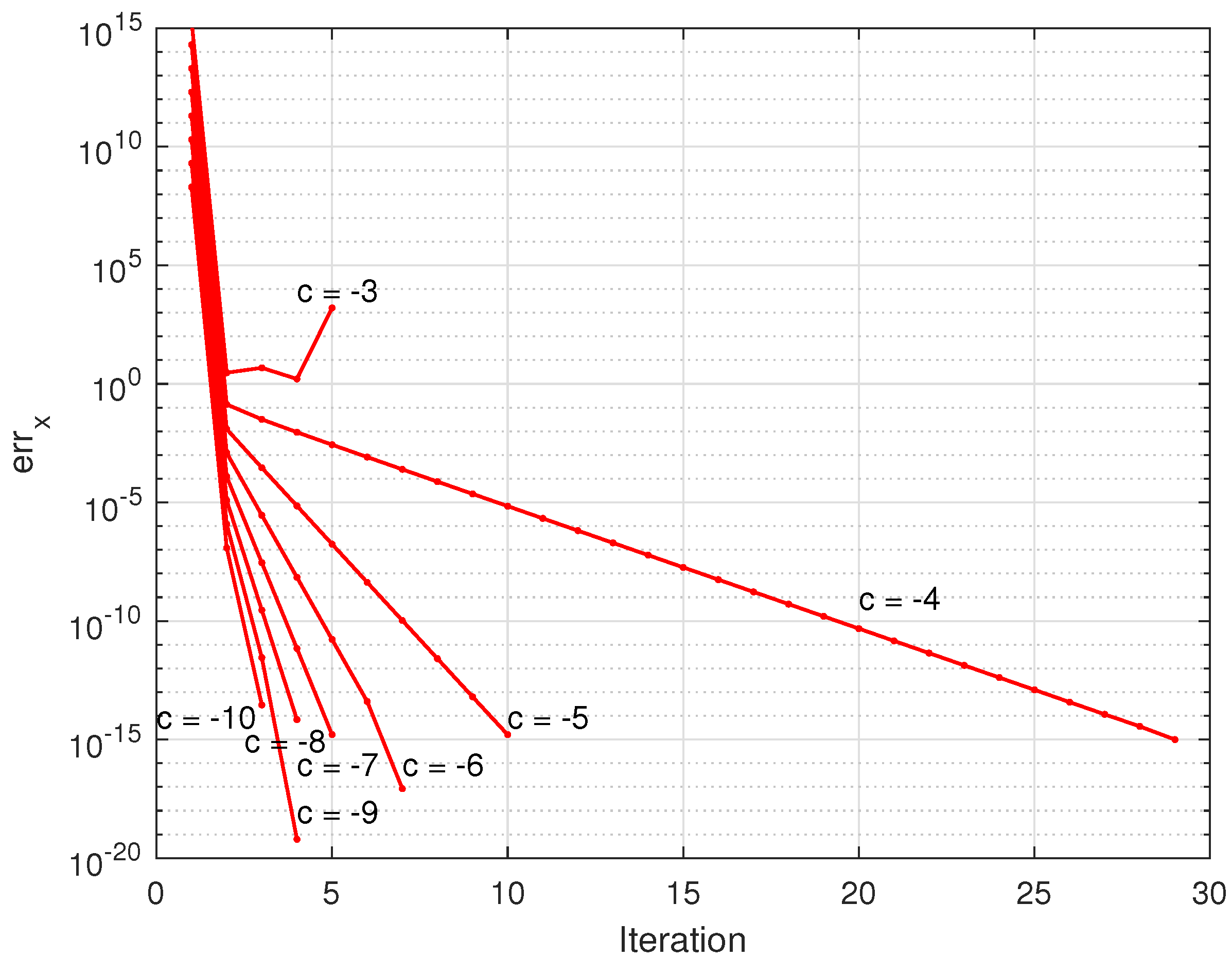
Figure 4.
Iterations for finding the global bounds of y.
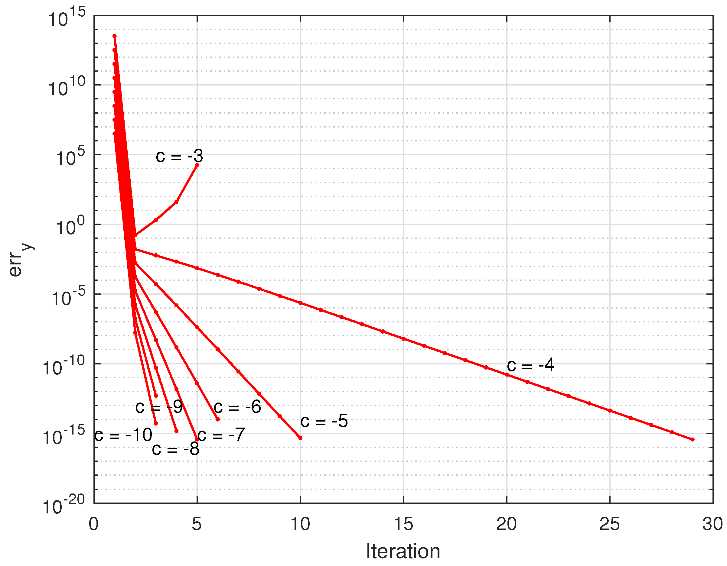
Figure 5.
Exact values of and the corresponding linear and nonlinear estimates as functions of the perturbation norm.
Figure 5.
Exact values of and the corresponding linear and nonlinear estimates as functions of the perturbation norm.
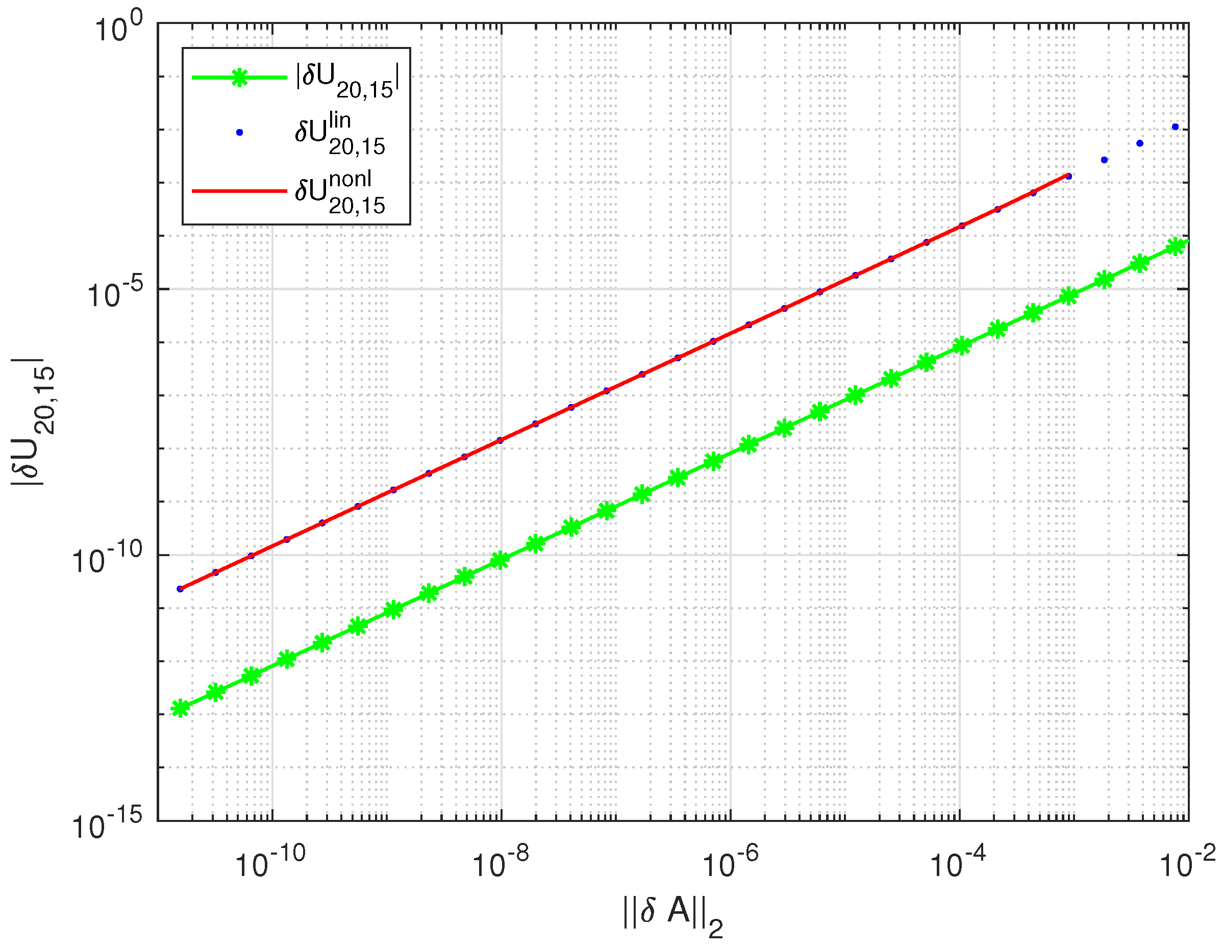
Figure 6.
Exact values of and the corresponding linear and nonlinear estimates as functions of the perturbation norm.
Figure 6.
Exact values of and the corresponding linear and nonlinear estimates as functions of the perturbation norm.
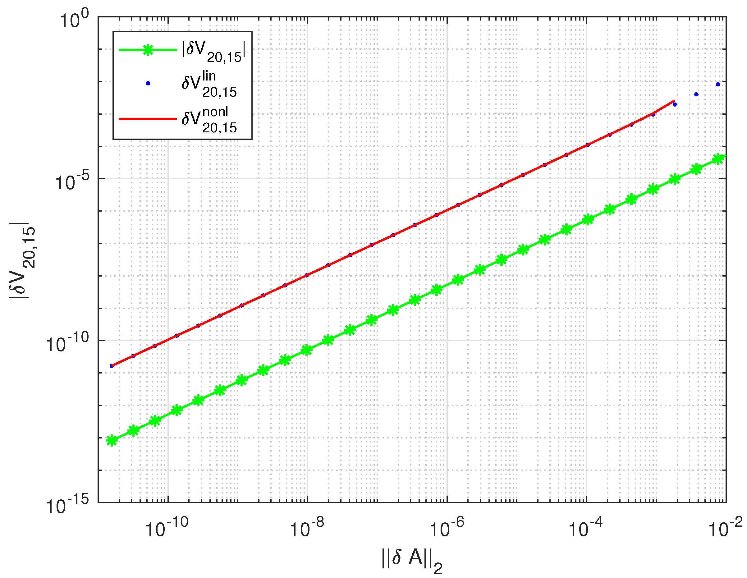
Figure 7.
Exact values of and the corresponding linear and nonlinear estimates as functions of the perturbation norm.
Figure 7.
Exact values of and the corresponding linear and nonlinear estimates as functions of the perturbation norm.
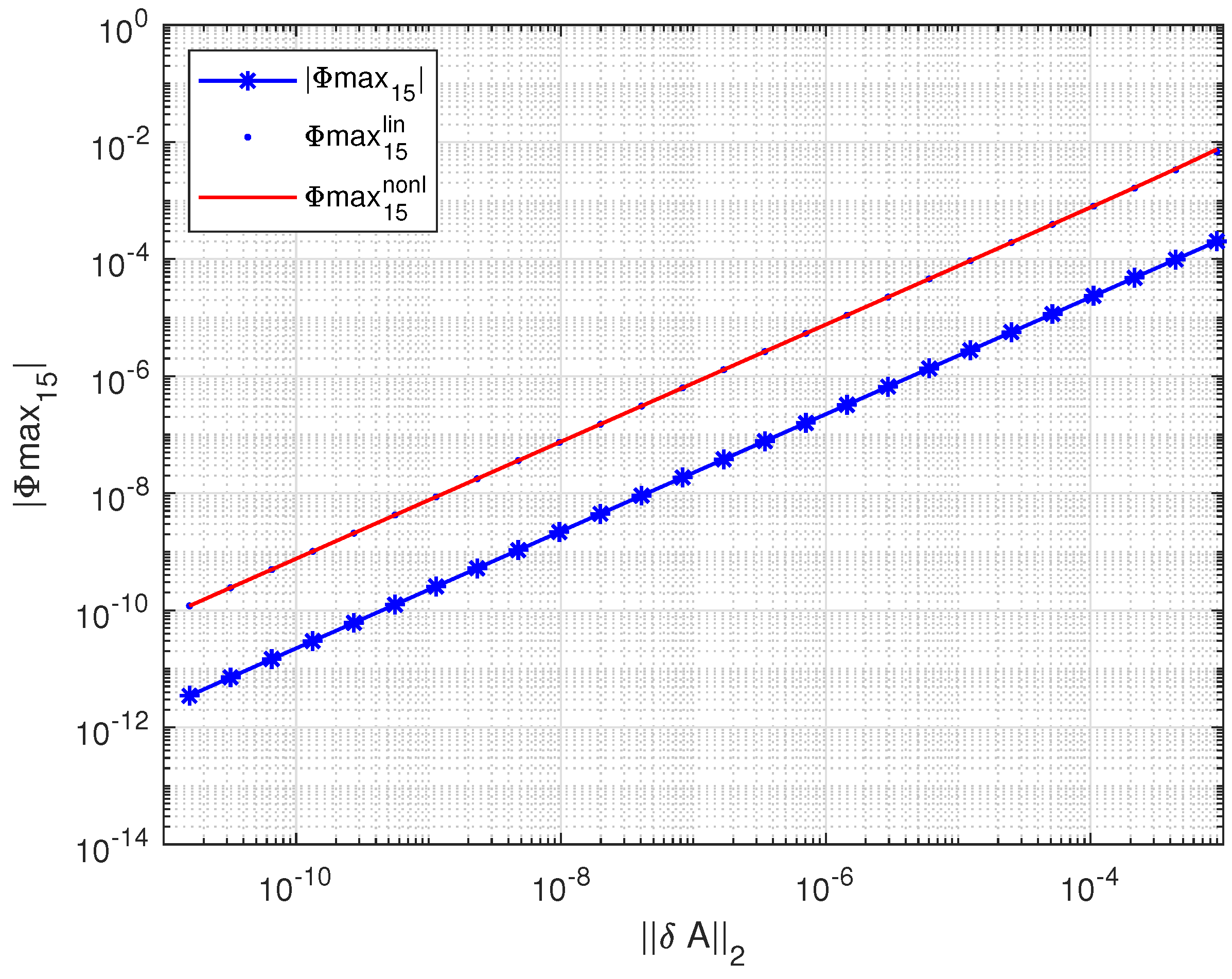
Figure 8.
Exact values of and the corresponding linear and nonlinear estimates as functions of the perturbation norm.
Figure 8.
Exact values of and the corresponding linear and nonlinear estimates as functions of the perturbation norm.
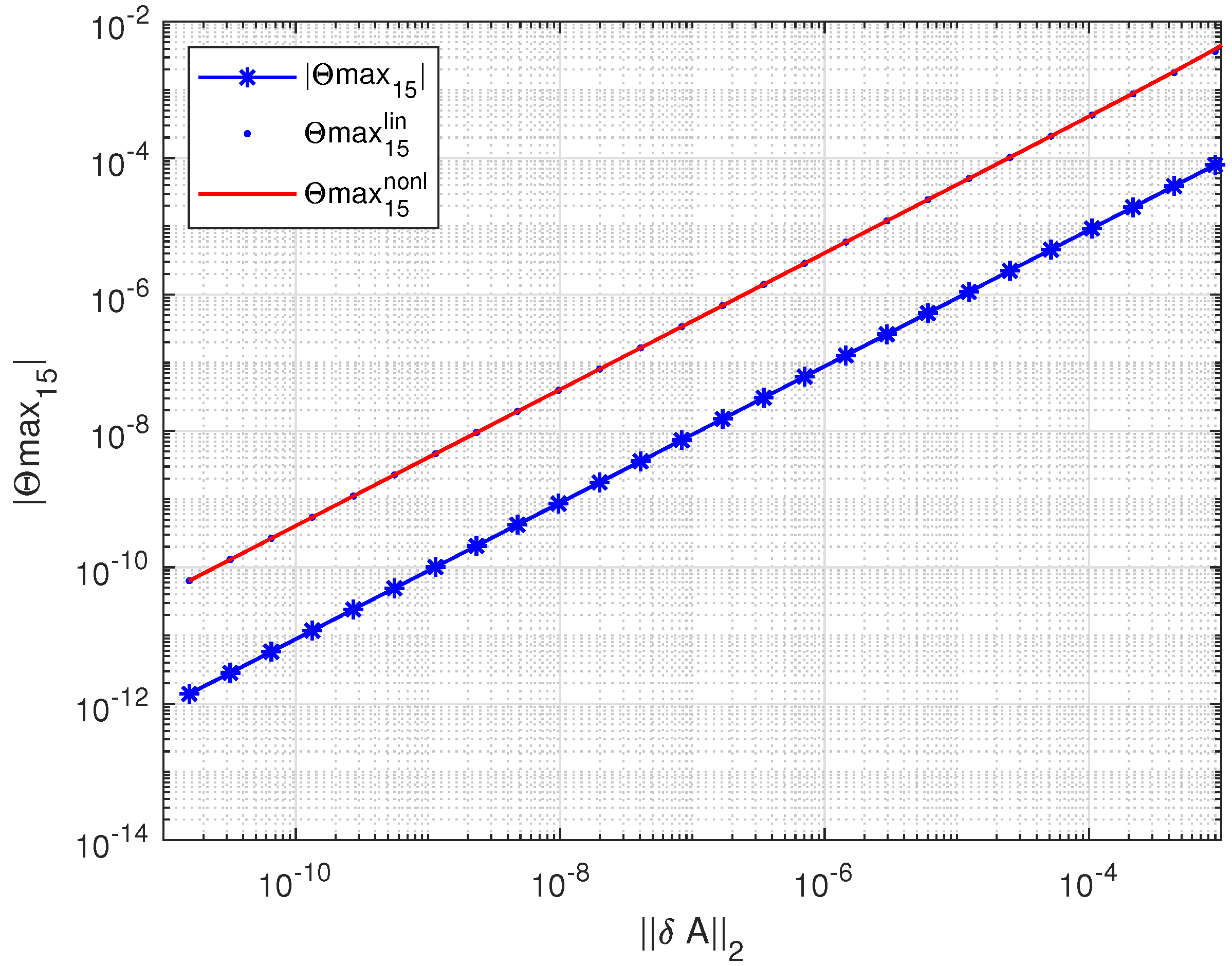
Figure 9.
Perturbations of the singular values and their nonlinear bounds for .
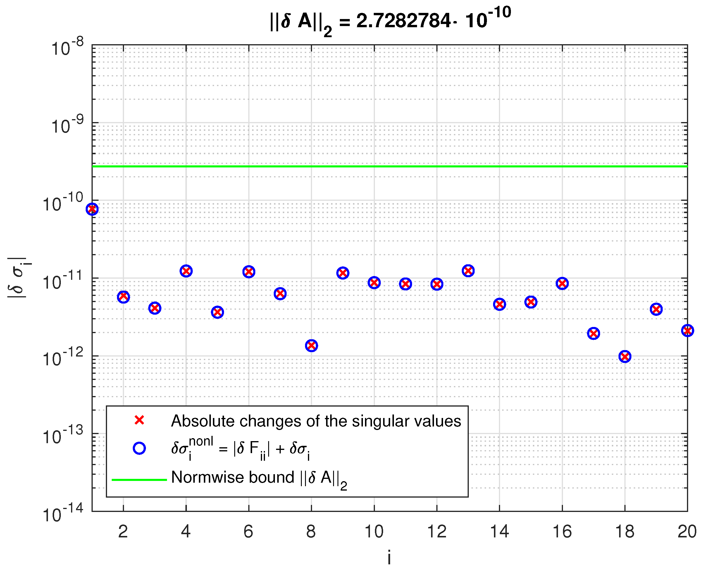
Figure 10.
Perturbations of the singular values and their nonlinear bounds for .
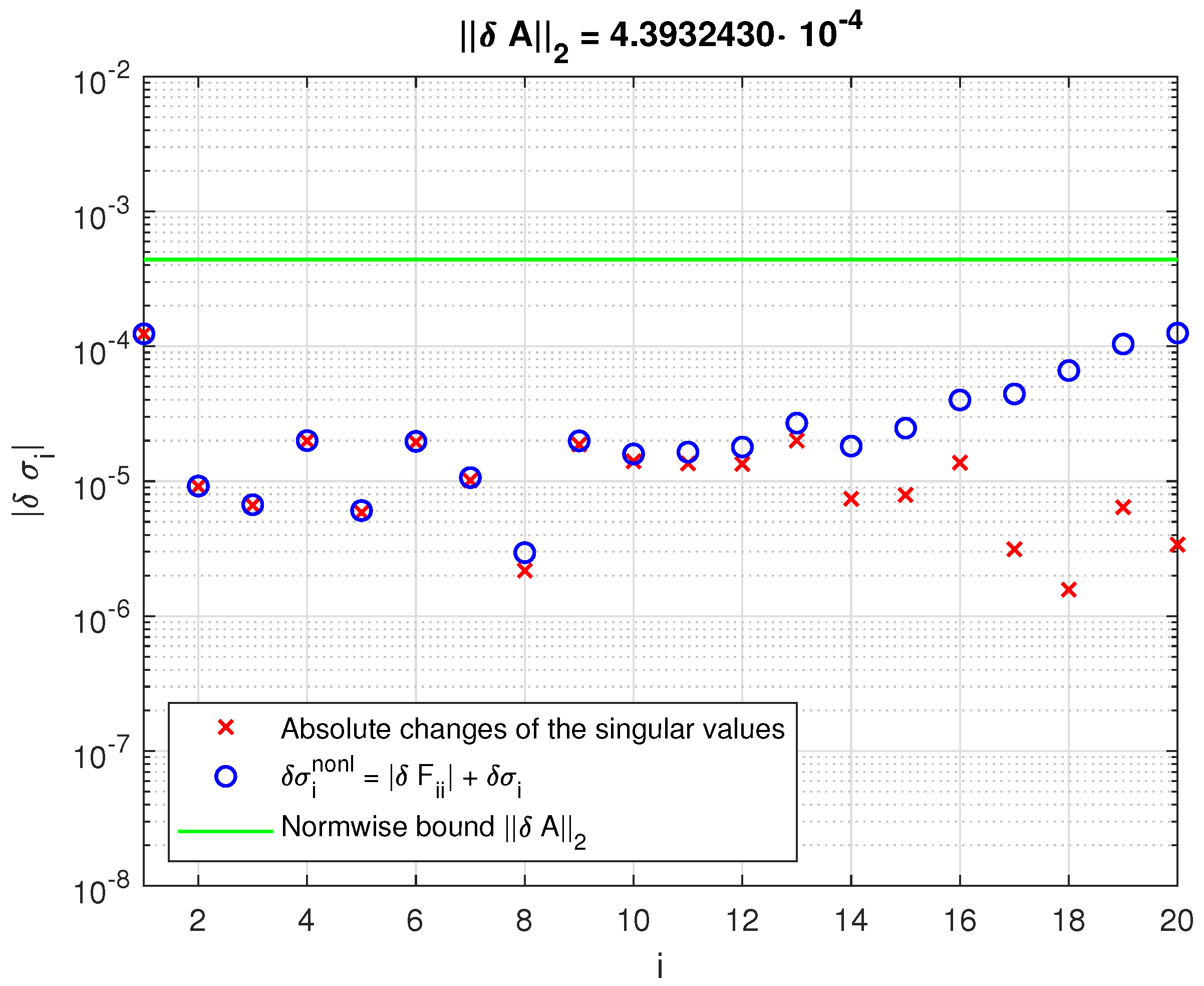
Figure 11.
Values of and the corresponding linear estimates.
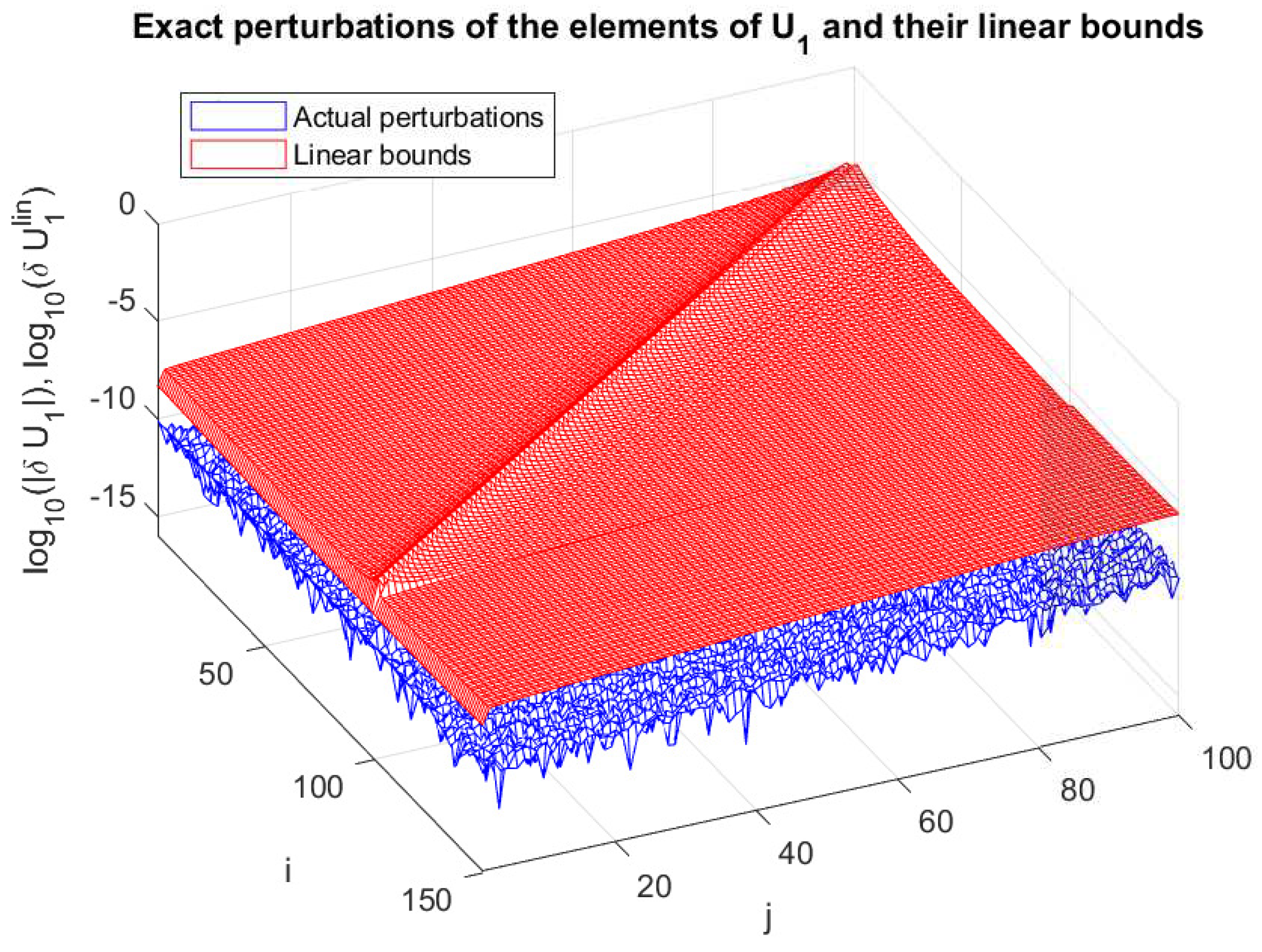
Figure 12.
Values of and the corresponding linear estimates.
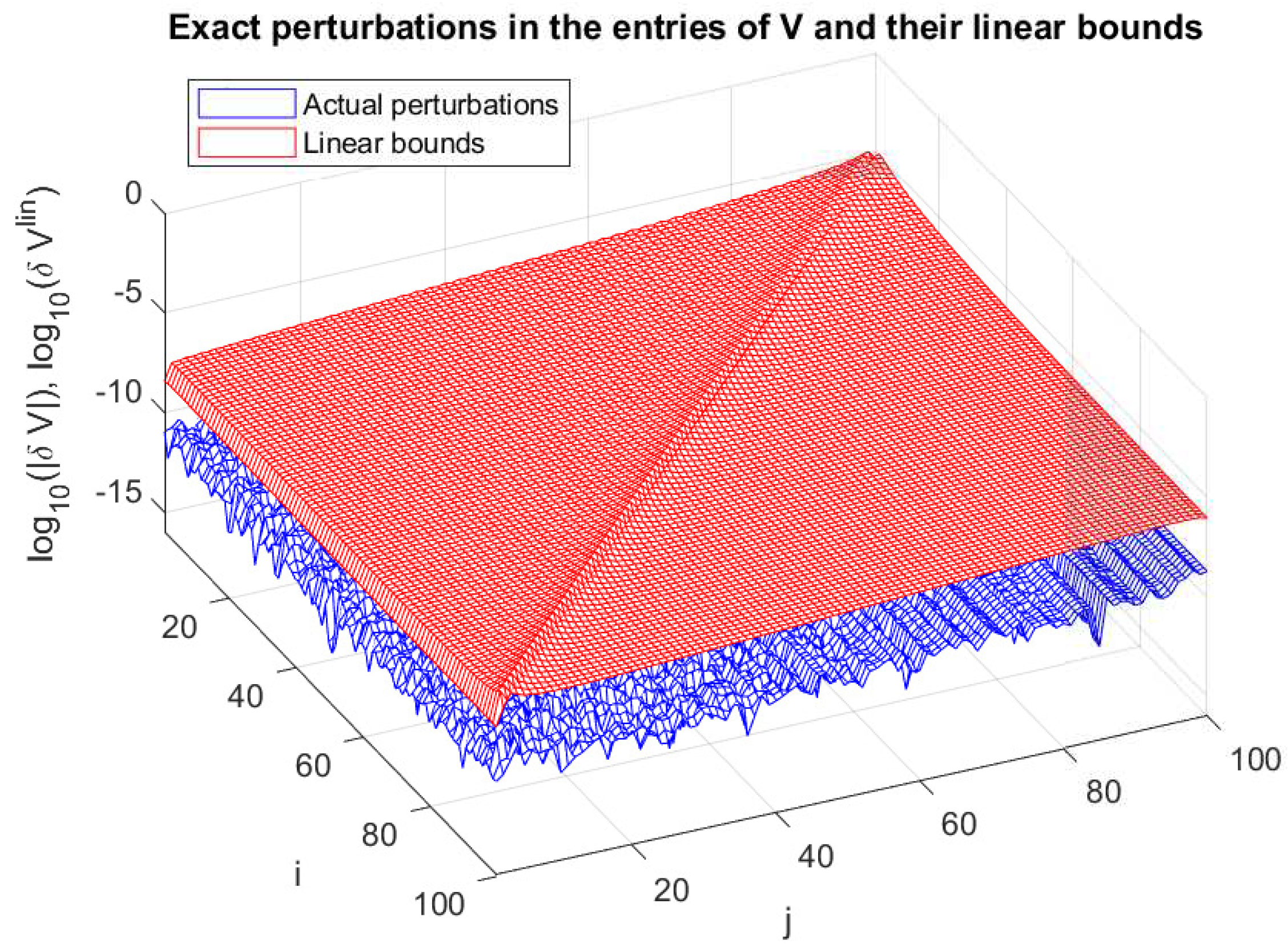
Figure 13.
Perturbations and perturbation bounds of the singular values.
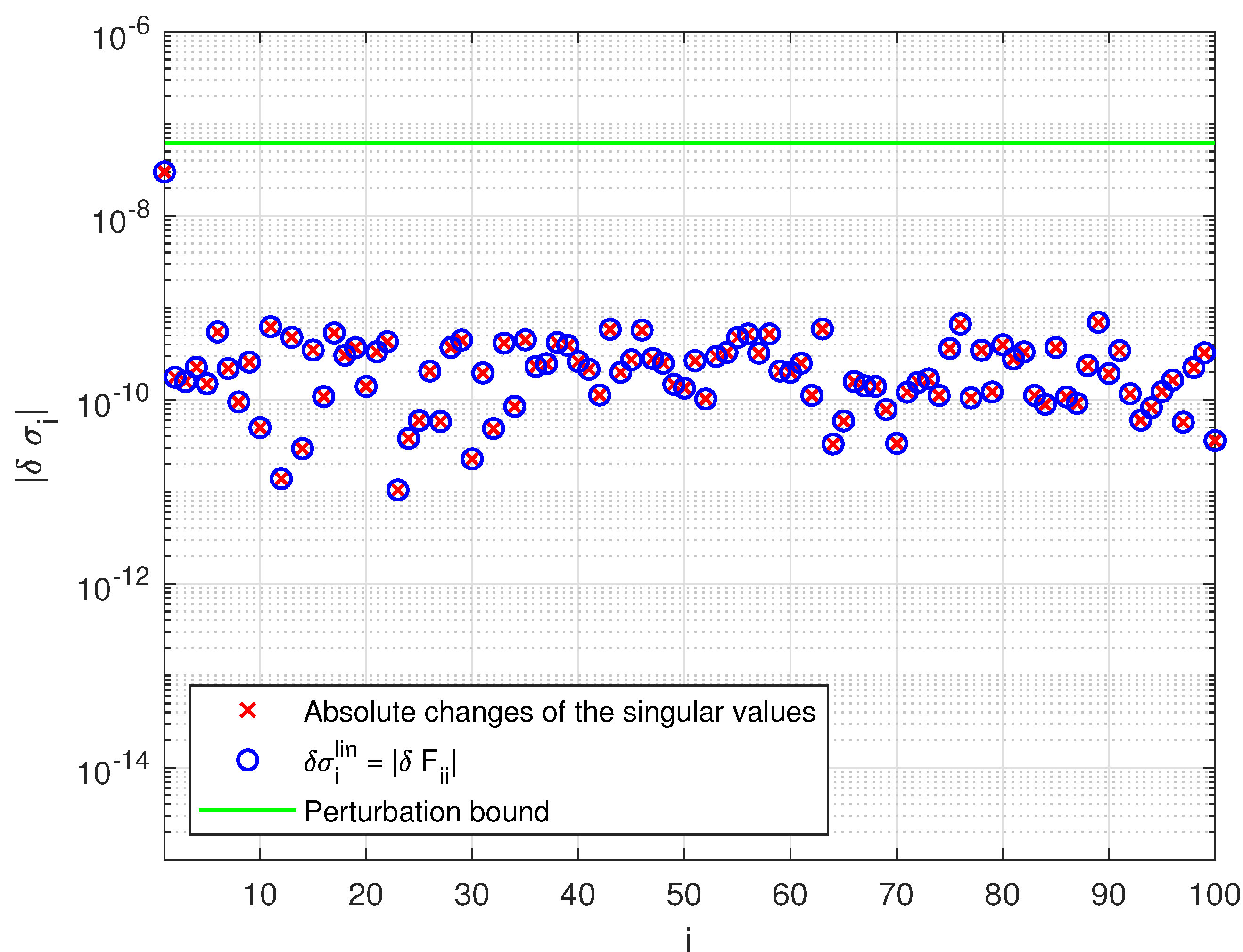

Table 1.
Exact perturbation parameters related to the matrix and their linear estimates.
| c | ||||
|---|---|---|---|---|
Table 2.
Exact perturbation parameters related to the matrix and their linear estimates.
| c | ||||
|---|---|---|---|---|
Table 3.
Perturbations of the singular values and their linear estimates.
| c | |||
|---|---|---|---|
Table 4.
Sensitivity of the singular subspaces.
| c | |||
|---|---|---|---|
| c | |||
Table 5.
Convergence of the global bounds and higher order terms.
| c | Number of iterations | |||
|---|---|---|---|---|
| 4 | ||||
| 4 | ||||
| 5 | ||||
| 5 | ||||
| 7 | ||||
| 10 | ||||
| 29 | ||||
| No convergence | - | - |
Table 6.
Global bounds of x and y.
| c | ||||
|---|---|---|---|---|
Table 7.
Perturbations of the singular values and their nonlinear estimates.
| c | |||
|---|---|---|---|
Table 8.
Nonlinear sensitivity estimates of the singular subspaces.
| c | |||
|---|---|---|---|
| c | |||
Disclaimer/Publisher’s Note: The statements, opinions and data contained in all publications are solely those of the individual author(s) and contributor(s) and not of MDPI and/or the editor(s). MDPI and/or the editor(s) disclaim responsibility for any injury to people or property resulting from any ideas, methods, instructions or products referred to in the content. |
© 2023 by the authors. Licensee MDPI, Basel, Switzerland. This article is an open access article distributed under the terms and conditions of the Creative Commons Attribution (CC BY) license (http://creativecommons.org/licenses/by/4.0/).
Copyright: This open access article is published under a Creative Commons CC BY 4.0 license, which permit the free download, distribution, and reuse, provided that the author and preprint are cited in any reuse.


