Submitted:
10 September 2025
Posted:
11 September 2025
You are already at the latest version
Abstract
A condition-based maintenance modeling approach for a multi-state system under competing failures and imperfect repairs is proposed. The multi-state system will experience three states (normal, defective and failed) through its lifecycle caused by two competing failure processes, i.e., natural degradation and external shocks. If the system becomes defective, an imperfect repair is adopted to restore the system to a normal state. Firstly, imperfect repairs aimed at addressing defects are mathematically characterized, based on which two kinds of system renewal scenarios and corresponding occurrence probabilities are simulated and derived, respectively. Subsequently, the cost of downtime caused by hidden failures are deduced. Then, a maintenance model of the expected cost rate is constructed and the optimal inspection period that minimizes the expected cost rate is determined. Finally, the correctness and effectiveness of the constructed maintenance model are verified by a numerical example.
Keywords:
multi-state system
; maintenance model
; competing failures
; imperfect repair
; inspection strategy
1. Introduction
In classical reliability theory, systems are typically modeled as having two distinct states: perfect functioning and complete failure. However, this binary representation is often too simplistic to capture the behavior of complex real-world systems. Many industrial systems, such as those in electrical power generation, aerospace, production, and manufacturing, exhibit multiple performance levels between full functionality and total failure. These systems are known as multi-state systems (MSSs) [1,2,3,4].
The evolution of the system state is influenced both internal degradation and external shocks. Internal degradation generally results from the operational workload of the system. For instance, in a battery, power is supplied through chemical reactions between internal chemicals, and degradation occurs over time as these chemicals are gradually consumed. External shocks, on the other hand, stem from random environmental damages, including both natural and human-induced factors. Examples include overheating or over-voltage conditions that can abruptly worsen the system’s state. Both internal degradation and external shocks can lead to system failure, though they manifest differently. Failures due to internal degradation are often termed soft failures, characterized by a gradual decline in performance until the system can no longer meet operational requirements. This includes phenomena such as mechanical wear and tear or the aging of insulating materials. In contrast, hard failures result from external shocks and involve a sudden loss of function, such as device breakdowns or short circuits. The system is considered failed when either of these competing failure modes occurs first. Moreover, multi-state degradation is commonly observed in systems subject to competing failure processes prior to the final failure [5].
Maintenance is crucial for enhancing the reliability and safety of engineered systems. Both academic research and engineering practice have demonstrated that condition-based maintenance (CBM) offers distinct advantages in reducing or preventing failures compared to other preventive maintenance strategies [6]. With the rapid advancement of sensor technology and signal processing methods, the benefits of CBM in supporting maintenance decisions have become even more pronounced. The first step in CBM involves assessing the system state, followed by appropriate maintenance actions based on the assessment.
Numerous studies have explored CBM for MSSs subject to two competing failure modes, with a primary focus on developing and optimizing inspection and maintenance models. A key contribution of these works lies in their modeling approaches, where the formulated models are largely influenced by inspection and maintenance policies. In practice, however, inspection quality is often compromised by factors such as measurement errors, sensor degradation, and other uncertainties, meaning inspections are typically imperfect. The issue of imperfect inspection in MSSs with competing failure modes has been addressed by several researchers [7,8]. In these studies, maintenance actions based on inspection outcomes predominantly involved replacement.
Nevertheless, replacement is often more costly than repair. Especially in addressing partial system defects, imperfect repair strategies may be more suitable, as they allow maintenance personnel to control the extent of reliability improvement, making repair levels a decision variable [9,10]. Despite its potential, imperfect repair has not received sufficient attention within CBM frameworks for MSSs subject to competing failure modes.
Motivated by both theoretical foundations and industrial practice, this study develops CBM models for MSSs with two competing failure modes, with the aim of deriving an optimal inspection policy. The system undergoes gradual degradation, leading to a decline in performance from a normal state to a defective state, and eventually to failure. Additionally, the system is exposed to random shocks from the external environment. A sudden failure occurs if the load of any shock exceeds a certain threshold.
Periodical inspections are conducted to monitor the system state. Based on the inspection results, the operator decides whether to perform maintenance. When a defect is identified, the system undergoes an imperfect repair, modeled by a proportional age reduction approach. This repair restores the system from a defective state to a normal state but does not return it to an “good as new” condition. If a failure whether due to gradual degradation or a fatal shock is detected, a failure-based replacement is performed. Furthermore, if the system remains in a normal state after a predetermined number of inspections, an age-based preventive replacement is conducted. Both types of replacement restore the system to an as-good-as-new state.
The probabilities associated with these two system renewal scenarios under imperfect repair are first derived. Based on these, a CBM model for the expected cost rate is formulated. To evaluate the performance of the proposed model, optimization and sensitivity analysis are carried out. The results demonstrate that the optimal inspection policy can be determined by minimizing the expected cost rate. Moreover, improving the repair effectiveness can significantly reduce inspection frequency and lower maintenance costs.
In summary, the main contributions of this study are as follows:
- A novel CBM model is developed for MSSs subject to two competing failure modes, incorporating imperfect repairs. The proposed methodology captures multiple system states, diverse failure modes, and imperfect maintenance actions, offering enhanced realism and addressing greater practical complexity.
- The model explicitly incorporates imperfect repair to better represent the actual impact of maintenance on system condition. Results underscore the importance of considering imperfect repair, as it significantly affects both the optimal inspection policy and the minimal expected cost rate.
- A comprehensive sensitivity analysis is conducted to examine how the optimal inspection policy responds to changes in key parameters. The findings provide valuable managerial insights that can support effective maintenance decision-making for real-world MSSs exposed to competing failure mechanisms.
The structure of the paper is organized as follows. Section 2 provides a review of the related literature. In Section 3, we present a detailed description of the system and the underlying assumptions. Section 4 develops the CBM model for the expected cost rate, incorporating the derived probabilities of imperfect repair, failure-based corrective replacement, and age-based preventive replacement, along with the computed costs associated with downtime. The solution approach for determining the optimal inspection interval and the minimum expected cost rate is introduced in Section 5. Section 6 offers a numerical example to demonstrate the application of the proposed model and presents a sensitivity analysis. Finally, Section 7 summarizes the main conclusions and suggests potential directions for future research.
2. Literature Review
In this section, we first focus on studies about MSSs. Then, we discuss studies about maintenance policies for MSSs. Finally, we introduce papers on imperfect repair for MSSs.
2.1. Research Topics on MSSs
A substantial body of research has been dedicated to MSSs, with major efforts concentrated in areas such as reliability analysis [11,12,13], resilience analysis [14,15,16], and maintenance policies [17,18,19]. For example, Janada et al. [20] developed a new design of Angular Control Chart to monitor the reliability of MSSs, whose failure data can be modeled by any continuous probability distribution. Lz transformations have been widely used in the reliability modeling of MSSs. To solve the problem of complex calculations due to the dense random combination of multi-state performance parameters in the Lz transformation, Zheng et al. [21] defined a screening function before the Lz transformation and combined with the performance threshold to screening the state performance parameters in advance. Mi et al. [22] introduced a reliability analysis method for complex MSSs with epistemic uncertainty, which was quantified by adding an uncertain state of root nodes in the multi-state evidential network. Tan et al. [23] focused on a MSS which is exposed to disruptive events and developed a comprehensive resilience modeling and quantifying framework based on Markov processes. To have a more comprehensive understanding of the characteristics of the system, Dui et al. [24] investigated the transient resilience evaluation for systems subjected to competing failures. The overall resilience of the system was introduced based on the multi-state division of the system, the resistibility index, absorbability index and recoverability index, and then a reliability and a cost-based resilience model was proposed.
2.2. Maintenance of MSSs
In the study of MSSs, maintenance strategies represent a prominent research focus. Timely and effective maintenance planning can restore aging systems to improved conditions, thereby preventing unexpected failures and mitigating undesirable consequences during operation [25]. Chen et al. [26] proposed a joint optimization model of fleet-level sequential selective maintenance and repairpersons assignment under flow dependency and uncertain maintenance duration. In the proposed optimization model, the reliability of multi-state manufacturing systems was incorporated. Ma et al. [27] developed a new selective maintenance model by integrating maintenance decision and task assignment planning for multi-unit systems executing multiple missions and a cooperative co-evolutionary genetic algorithm was tailored to solve the joint optimization problem. Results through a numerical example and an air defense system showed that the proposed method can efficiently improve the success probability of future missions by integrating selective maintenance and task assignment.
In recent years, advancements in sensing technologies have significantly enhanced the application of condition monitoring data in maintenance practices, leading to increased effectiveness and adoption of CBM strategies. As a result, research on CBM for multi-state systems has attracted growing interest [28,29,30,31]. For example, Cao et al. [32] designed a condition-based inspection policy to capture the states of a multi-state deterioration system timely, based on which a new CBM policy for systems subject to multi-state deterioration and random shock were proposed. Zhao et al. [33] focused on the effect of environmental factors on system failure behavior and maintenance decisions and investigated the optimal joint inspection interval, CBM, and loading policies for systems operating in a random shock environment. Zhang et al. [8] constructed a CBM model for a three-state system subject to competing and hidden failures, where periodical inspection was utilized to identify all states of the system. Wang and Zhu [34] considered the joint optimization of periodic condition-based replacement of components and inventory control for a k-out-of-n: F system, whose degrading components have multiple statuses and are non-repairable. Tang et al. [35] considered a multistate deteriorating system whose states are hidden but partially observable and determined the optimal maintenance and spare parts inventory ordering policy. In this study, a partially observable Markov decision process and a heuristic search value iteration algorithm were respectively adopted to model the problem and solve the optimization problem.
2.3. Imperfect Repair in Maintenance Policies of MSSs
Over the past few decades, significant attention has been devoted to the concept of imperfect repair. It refers to a maintenance intervention that falls between perfect repair and minimal repair. A perfect repair restores an item to an “as good as new” condition, while a minimal repair returns it to an “as bad as old” state. Researchers have increasingly incorporated imperfect repair into maintenance models for MSSs. Dong et al. [36] scheduled an imperfect maintenance policy for a single unit MSS. A CBM action and a corrective maintenance (CM) activity were incorporated in each operation stage, and the CBM was assumed to be a minimal repair and the effectiveness of CM was assumed to be imperfect. Finkelstein and Cha [37] investigated a new approach to modelling the imperfect repair and described the corresponding imperfect repair processes for items with observable degradation process. The random virtual age was introduced to define the state of an item after an imperfect repair, which reduced degradation of an item on failure to some intermediate level. In the research by Liang et al. [38], the states of the system before repair were categorized into three classes based on its internal degradation level: failure, major defect and minor defect with three corresponding thresholds. The corresponding repairs were carried out to reduce the system’s degradation to different levels. If the internal degradation level of the system was recognized as minor defect, an imperfect repair was implemented to scale down the degradation level below the minor defect threshold. If the degradation level was identified as major defect, an upgraded imperfect repair was executed. Otherwise, if the degradation was beyond the failure threshold, replacement would be carried out. Ultimately, a novel hierarchical imperfect maintenance structure was introduced, and a multi-variable repair cost model was constructed. Tang et al. [39] considered imperfect inspection and imperfect repair for a system subject to a three-stage degradation process. The concepts of virtual age and the improvement factor were adopted to characterize the imperfect repair effect. The case of a steel converter plant was applied to verify the effectiveness of the proposed model. Chen and Zhao [40] proposed a maintenance optimization method that is applicable to dependent two-component systems subject to degradation and imperfect repair. A random-effect imperfect repair model was established to model the degradation process and maintainability of components. The study discovered that the characteristics of imperfect repair can considerably influence the optimal policies. Hu et al. [41] proposed a CBM model for multi-state systems that operate under time-varying environmental condition, whose evolution was described by a Markov process. Both imperfect maintenance and replacement actions were considered in the constructed CBM model. The inspection interval, preventive maintenance threshold and number of imperfect maintenance actions in a replacement cycle were jointly determined to minimize the long-run average cost.
Existing research has primarily focused on MSSs influenced by a single failure mode, whereas the imperfect repair of MSSs subject to two competing failure modes has received comparatively little attention.
3. System Description and Basic Assumptions
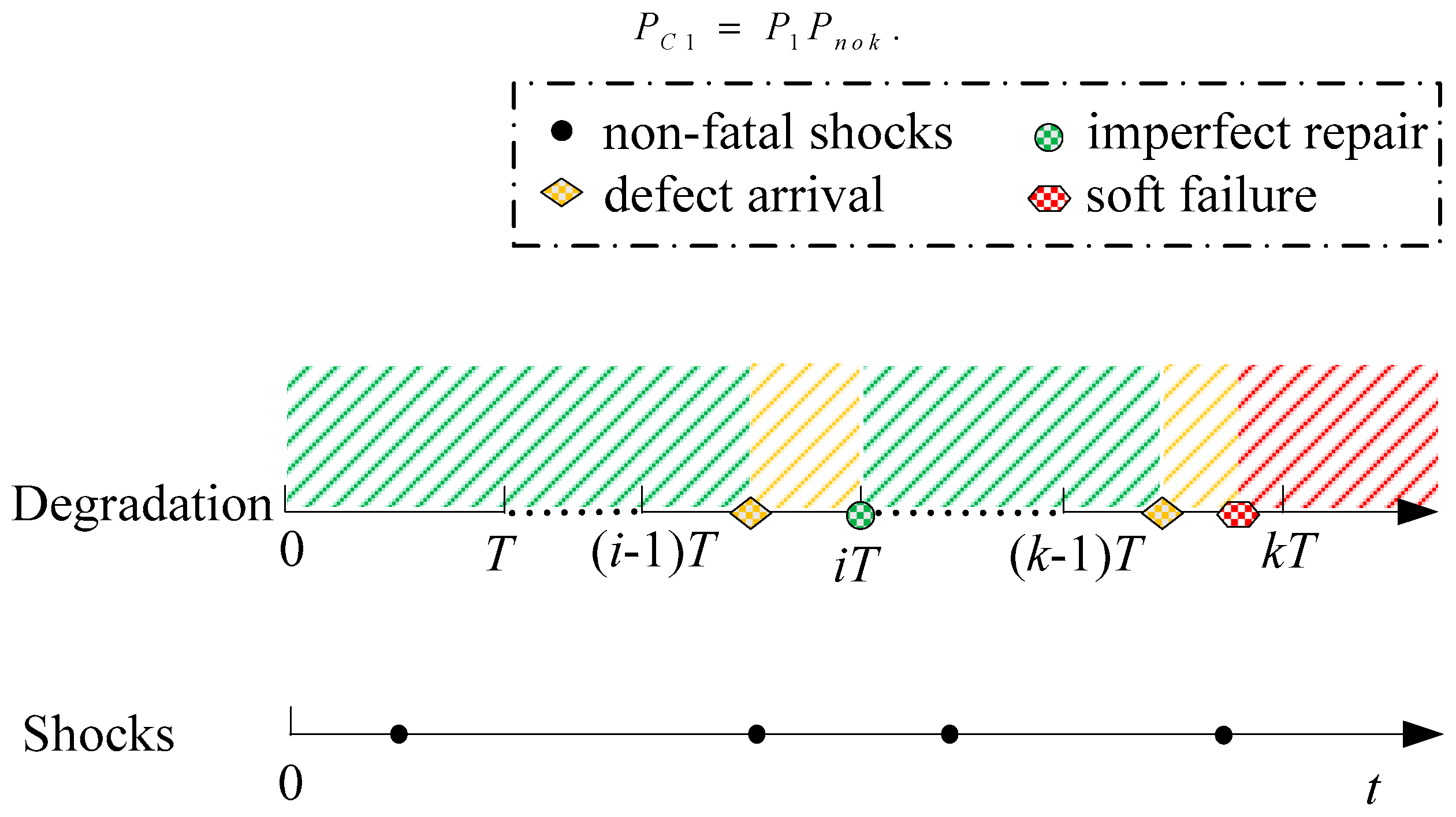
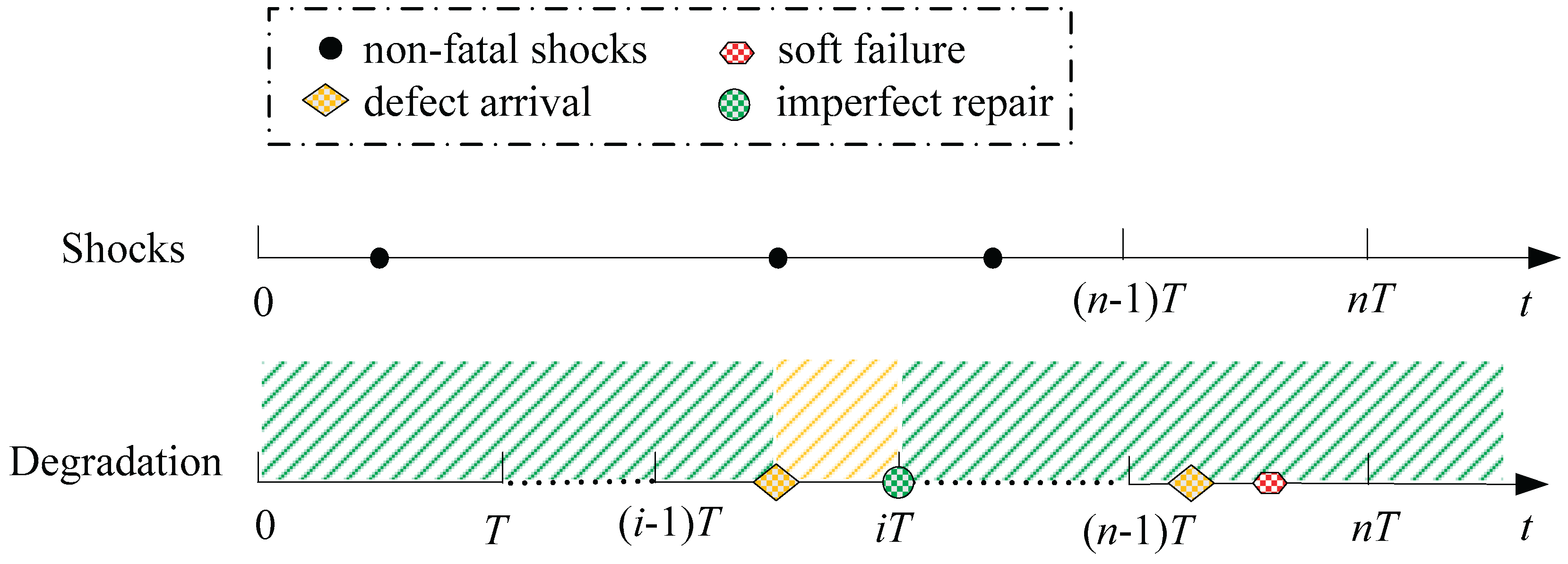
In this paper, a MSS subject to two competing failure modes with hidden failures is taken as a research object to explore its maintenance modeling methodology. When there are no external shocks, it is assumed that the system goes through three states during the degradation process: normal, defective, and failed. As shown in Figure 1, initially, the system is in a normal state. As the system’s operational time increases, its performance gradually degrades, entering a defective state. Eventually, the core functions are lost, resulting in system failure.
However, the system will inevitably be affected by external shocks. As shown in Figure 2, suppose that shocks reach the system at and their loads are W1, W2, W3, ..., Wj. If the magnitude Wj of the jth shock (where j =1, 2, …, ∞) exceeds the sudden failure threshold D, the system is deemed to have experienced a sudden failure. The degradation failure and sudden failure compete with each other, and the failure mode that occurs first ultimately leads to system failure.
In this paper, the maintenance model of the MMS under competing failures is constructed based on the CBM strategy, which is based on the state of the system to formulate the appropriate maintenance action. The state of the MSS needs to be identified through inspection. Among various inspection technologies, periodic inspection is widely used due to its ease of implementation and effectiveness in improving system performance. Therefore, this article adopts a periodic inspection strategy to identify the state of the system and then arranges corresponding maintenance activities for the MSS based on the detected states. Maintenance behavior based on the system state consists of the following 3 main types: (1) If the system is identified as a defective state at the kth (k =1, 2, ..., n) inspection, an imperfect repair is performed on the system. (2) At the kth (k = 1, 2, ..., n) inspection, if the system is detected to have entered a failed state, a corrective replacement is implemented to restore the system as new. (3) If the system is still normal at the nth inspection, a preventive replacement is performed to restore the system as new to enhance the system’s ability to withstand external shocks.
The following research hypotheses are proposed to better construct a maintenance model for the MSS subject to competing failures and imperfect repairs.
Assumption 1. The MSS is susceptible to hidden failures, which result in downtime and consequent economic loss.
Assumption 2. Repairs for system defects are considered imperfect repairs. The effect of repair in engineering practice is usually imperfect. A system can seldom be restored to an “as-new” state but is instead returned to a condition intermediate between “as new” and “as old”.
Assumption 3. Degradation failure and sudden failure are independent, with system failure resulting from the competition between these two modes. The degradation process is modeled using a delay-time approach, while the sudden failure process is described by a homogeneous Poisson process.
Assumption 4. The system’s duration in the normal and defective states are random variables, denoted by X and Y, respectively, with probability density functions fX(x) and fY(y). Shocks arrive at the system with intensity λ, and their magnitudes are independent and identically distributed normal random variables, .
Assumption 5. The time for inspection, repair, preventive replacement, and corrective replacement is assumed to be negligible.
4. Maintenance Modeling for MSSs Subject to Competing Failure Processes and Imperfect Repairs
There is a critical trade-off in maintenance scheduling: overly frequent inspections waste resources, but excessively long intervals may cause missed opportunities for timely repairs. The objective of this study is to establish the optimal inspection interval for the MSS through the development and optimization of a maintenance model, with the goal of minimizing the total maintenance cost over the long term.
Two of the three maintenance behaviors mentioned in Section 3 will renew the system. The first system renewal scenario is triggered upon detecting a system failure at the kth (k=1, 2, …, n) inspection, leading to a corrective replacement. The second type of system renewal scenario is a preventive replacement when the system is inspected as normal until the nth inspection. Let the period inspection interval be T. If the time interval between two consecutive replacements is defined as a renewal cycle, the system renewal cycle length for the first system renewal scenario is kT (k = 1, 2, …, n), while it equals nT for the second system renewal scenario.
Let the occurrence probabilities of a corrective replacement and a preventive replacement be Pcor(L=kT) (k=1, 2, …, n) and Ppre(L=nT) respectively. Then, the expected length of the system renewal cycle can be expressed by the following equation.
Different system renewal scenarios correspond to different renewal cycle lengths and are associated with distinct maintenance costs. For the first renewal scenario, the total cost from system startup to failure comprises the expenses for k (k = 1, 2, ..., n) inspections, any imperfect repairs conducted prior to failure, one corrective replacement and the downtime costs attributable to hidden failures. Similarly, the costs incurred during a renewal cycle initiated by a preventive replacement primarily include the expenses for n inspections, those for any imperfect repairs performed before the nth inspection, and the cost of one preventive replacement.
Denote the unit inspection cost, imperfect repair cost, preventive replacement cost, and corrective replacement cost as CI, CR, CP, and CC, respectively. The cost of downtime due to hidden failures is denoted by CD. Assume that the probability of identifying a system defect at the ith inspection (where i = 0, 1, ..., k-1) and subsequently addressing it with an imperfect repair is P(T, i). Based on these cost parameters, the probability of an imperfect repair, and the probabilities associated with the two system renewal scenarios, the expected total cost per renewal cycle can be derived as follows.
where represents the aggregate cost of imperfect repairs undertaken for defects prior to a corrective replacement, and represents the total cost of all imperfect repairs performed prior to a preventive replacement.
Based on Equations (1) and (2), the expected cost rate model for the condition-based maintenance of the MSS is constructed as follows.
The primary objective of this study is to determine the optimal inspection interval T* that minimizes the expected cost rate function ECR(T). As shown in Equations (1) and (2), the maintenance model involves four key unknown terms: the probability of imperfect repair P(T, i), the probability of corrective replacement Pcor(L=kT), the probability of preventive replacement Ppre(L=nT), and the cost of downtime due to hidden failures CD.
By examining system renewal scenarios, it is evident that the system may degrade into defective states and undergo imperfect repairs before either corrective or preventive replacement occurs. Consequently, the derivation of the corrective replacement probability Pcor(L=kT) and the preventive replacement probability Ppre(L=nT) depends on the probability P(T, i) of imperfect repairs. Thus, the subsequent analysis proceeds as follow. First, the probability P(T, i) of imperfect repairs for system defects is derived. Next, the probabilities Pcor(L=kT) and Ppre(L=nT) are computed based on P(T, i). Subsequently, the downtime costs CD due to hidden failures are analyzed and evaluated. Finally, the maintenance model of the system is formulated by integrating the explicit expressions of these four key terms with the relevant cost parameters.
4.1. Mathematical Modeling of Imperfect Repair for System Defects
In this study, repair activities are scheduled to address system defects. However, these repairs can only restore the system from a defective state to a normal operating state, rather than making it “good as new”. Such interventions are therefore considered imperfect. To model this imperfection, the proportional age reduction model is employed. This model is based on the premise that the (k+1)th repair only influences the system’s operating time between the (k+1)th and the kth repair.
Let be the time at which the kth repair is performed and the improvement factor of the repair. Then the (k+1)th repair reduces the virtual age of the system by . Therefore, the virtual age of the system at time t is given by
The virtual age defined in Equation (4) corresponds to the “normal age”, representing the actual duration during which the system remains in a normal state. This quantity exclusively influences the intensity function associated with the initiation of defects. Although an imperfect repair cannot restore the system to an “as good as new” condition, it entirely eliminates existing defects. As a result, the defective age of the system is reset to zero following each repair.
As illustrated in Figure 3, if a defect first occurs at time x1 and is identified at , the normal operating age of the system at that moment is x1, and its defective age is . Since inspections in this study are assumed to be perfect, the defect will be detected and repaired during the subsequent inspection, i.e., at time . The imperfect repair completely eliminates the defect and converts the accumulated defective age into normal operating age. Consequently, after the repair, the normal operating age of the system becomes , while the defective age is reset to zero.
If a system defect is detected at the ith inspection and is subsequently subjected to an imperfect repair, the density function of the defect initiation time X following this imperfect repair can be expressed as follows:
where .
Additionally, the probability of an imperfect repair following the ith inspection can be derived using the following expression.
where denotes the probability that the last imperfect repair was performed at time mT and .
4.2. Probability of Implementing a Corrective Replacement
The system renewal process can be categorized into two scenarios. They are respectively corrective replacement following system failure after the kth inspection (where k = 1, 2, ..., n) and preventive replacement performed if the system remains in a normal state up to the nth inspection. This section first derives the probability of a corrective replacement. A corrective replacement is triggered when the system fails at the kth inspection (k = 1, 2, ..., n). System failure may arise from one of three causes: (i) degradation failure, (ii) sudden failure, or (iii) a combination of both degradation and sudden failure.
- ⟡
- Case 1. System failure caused exclusively by degradation
In Case 1, the system degradation evolves such that the most recent defect occurs within the interval ((k-1)T, kT) for k = 1, 2, ..., n), and the system failure is detected during the kth inspection. Furthermore, the shock process affecting the system is characterized by the absence of any fatal shocks throughout the period (0, kT). Denoting the probability of this event by , it can be calculated as follows.
where λ represents the arrival rate of shocks, and D is the failure threshold of the shock process.
The probability of a corrective replacement, considering degradation only, is denoted by and can be expressed as follows.
Therefore, the probability of a corrective replacement triggered solely by degradation failure can be expressed as
Figure 4.
Evolution pattern of system state in Case 1.
- ⟡
- Case 2. System failure due solely to a sudden failure
Next, calculate the probability of a system failure attributable to a sudden failure. As illustrated in Figure 5 (Case 2), a sudden failure is identified at an inspection time kT (k = 1, 2, ..., n). Critically, at these same inspection intervals, the system’s degradation process may either be in a normal state (see degradation path (a) in Figure 5) or in a defective state (see degradation path (b) in Figure 5).
The shock process in Case 2 is characterized by the first fatal shock arriving between (k−1)T and kT, k = 1, 2, ..., n. This necessitates that no fatal shock occurs from time 0 to (k−1)T (event with probability PM, and at least one fatal shock occurs in the subsequent interval ((k−1)T, kT) (event with probability PN). Consequently, the overall probability for this shock scenario is
Define j1 as the total number of shocks reaching the system within the time period (0, (k−1)T). Then, PM can be computed as
The complement of the event of “at least one fatal shock reaches the system during ((k−1)T, kT)” is that “all shocks arriving at the system during ((k−1)T, kT) are non-fatal shocks”. Let j2 be the number of shocks during ((k − 1)T, kT). The probability PN can then be calculated as
The occurrence probabilities for the two evolutionary patterns of the degradation process can be calculated using the following two equations, respectively.
where .
Therefore, the overall probability of system failure attributable only to a sudden failure is given by the following expression.
- ⟡
- Case 3. System failure resulting from the combined effects of degradation failure and sudden failure
Finally, the probability of system failure resulting from the combined effects of degradation and sudden failure is computed. As illustrated in Figure 6, the shock process follows the same evolutionary pattern as in Case 2; its probability, denoted as Ph, is therefore given by Equation (10). In Case 3, the degradation process evolves such that the system transitions to a defective state within the interval ((k−1)T, kT), and a degradation failure is identified at the kth inspection. The probability of this degradation evolutionary pattern can be calculated using the following equation.
Consequently, the probability of system failure due to the concurrent occurrence of degradation failure and a sudden shock is given by
Following the preceding analysis, the probability for a corrective replacement action is therefore given by the sum of the three cases, which is equal to
4.3. Probability of Performing a Preventive Replacement
If the system remains in a normal state by the nth inspection, a preventive replacement should be performed. This is because, as service time increases, the system can function normally for progressively shorter durations, and its ability to withstand external shocks is significantly diminished. Consequently, there is a high likelihood of failure occurring in the near term, which could lead to substantial economic losses. A preventive replacement requires the satisfaction of two conditions. First, no fatal shock must have reached the system before time nT. Second, the degradation process must remain in a normal state at time nT.
Figure 7.
System state evolution under preventive replacement.
The probability of the event that no fatal shock arrives at the system before time nT is expressed as follows.
The probability of the evolutionary pattern of the degradation process can be calculated by
where .
Therefore, the probability of preventive replacement is equal to
4.4. Costs Associated with Operational Downtime
The expected cost of downtime resulting from hidden failures is the product of the cost per unit downtime and the expected downtime duration. Based on the Mean Past Life (MPL) method [42], it is assumed that the system fails at time Tf, . The resulting downtime length at the kth (k = 1, 2, ..., n) inspection is . Let Cd represent the cost of downtime per unit. The total cost of downtime due to hidden failures is then given by
The expected system downtime is calculated using the following procedure.
- Step 1. Manipulate the downtime length kT-Tf .
Let , then .
- Step 2. Derive based on the conditional expectation formula.
Let the cumulative distribution function and probability density function of Z be G(z) and g(z), respectively. Employing the conditional expectation formula from Equation (23), is expressed by Equation (24).
- Step 3. Derive the numerator and denominator of the right-hand term in Equation (24) separately.
First, the molecular is derived. Denote the cumulative distribution function and probability density function of the failure time as F(x) and f(x), respectively. Given that , it follows that and . Therefore,
Then, we derive the denominator .
Substituting Equations (25) and (26) into Equation (24) yields the following result.
Consequently, the costs associated with downtime losses attributable to hidden failures are calculated as follows.
where F(x) is the failure distribution function of the multi-state system, which depends on the distributions of the random variables X, Y and Wj.
5. Optimization of Inspection Scheduling to Minimize Expected Cost Rate
The primary objective of this paper is to determine the optimal inspection interval that minimizes the expected cost rate. This is achieved by developing and optimizing a maintenance model formulated as the expected cost rate, denoted ECR(T), where T represents the inspection interval and serves as the decision variable in the optimization framework.
Based on the probability of imperfect repair given in Equation (6), the probabilities of corrective and preventive replacements provided in Equations (18) and (21), and the cost contributions due to hidden failures derived in Equation (28), a comprehensive maintenance model of the multi-state system subject to competing failures and imperfect repair is constructed. The explicit expression of this model is presented in Equation (29).
Although ECR(T) is a univariate function of the decision variable T and has an explicit analytical expression, the diversity and complexity of its constituent terms make it impractical to derive a closed-form solution for T analytically. Therefore, this study employs a numerical approach to solve the maintenance model, thereby identifying the optimal inspection interval and its corresponding minimum expected cost rate. The simulation procedure is illustrated in Figure 8.
6. Numerical Example
Distribution system capacitor banks undergo continuous degradation from the start of their service life. In the initial stages, electrolyte consumption is minimal, and the system can be considered to be in a normal operating state. As the electrolyte depletes beyond a certain point, the capacitor bank enters a defective state. Once the electrolyte level falls below a critical threshold, the capacitor bank can no longer perform its intended function and eventually fails due to degradation.
In addition to inherent degradation, capacitor banks are also susceptible to external shocks, such as overvoltage or reverse voltage, which may cause sudden failure if the magnitude of any shock exceeds the sudden failure threshold. The condition of the capacitor bank can be assessed through periodic inspection, allowing for timely maintenance based on its identified state. This proactive approach helps ensure reliable performance and optimizes maintenance costs.
6.1. Maintenance Model Optimization and Analysis
Regularly inspect the capacitor bank at intervals of length T. If defects are identified, repair the capacitor bank to restore it to normal working condition. However, the repairs are imperfect, meaning they cannot restore the capacitor bank to an as-new state. Assume that before the first imperfect repair, the normal lifespan X and the delay time Y of the system follow Weibull distributions with shape parameters a1 and a2, and scale parameters b1 and b2, respectively. The probability density function and survival function of X are given by and , respectively. Similarly, the probability density function and survival function of Y are given by and , respectively.
Since imperfect repairs only affect the normal lifetime, it can be inferred from Equation (5) that after an imperfect repair is implemented at time iT, the probability density function of X becomes
Accordingly, the corresponding reliability function and lifetime distribution function are given by and , respectively. The parameters of the two Weibull distributions are respectively a1 = 1, a2 = 0.8, b1 = 2, b2 = 1.
The shock arrival intensity parameter (λ) for the system is 1. The mean () and variance () of the shock magnitudes are 5 and 4, respectively, and the sudden failure threshold (D) is 8. The minimum inspection interval is set to 1 month [43]. If defects are detected, the system undergoes imperfect repair with an improvement factor of ω = 0.8.
The failure time of the capacitor bank is assumed to follow a uniform distribution over the interval ((k-1)T, kT). The downtime cost per unit time, denoted as Cd, is 100 (in units of $100) [43,44]. The remaining cost parameters in the maintenance model are as follows.
- cost of a single inspection, CI = 10
- cost of an imperfect repair, CR = 40
- cost of a preventive replacement, CP = 60
- cost of a corrective replacement, CC = 800
Let n = 8. The expected cost rates under different inspection intervals can be calculated using Equation (29). As shown in Figure 9, the horizontal axis represents the inspection interval T, and the vertical axis represents the corresponding expected cost rates. As shown in Figure 9, when the repair improvement factor is set to ω = 0.8, the optimal inspection interval is 0.23 months. At this interval, the maintenance cost of the system is minimized, with a minimal expected cost rate of $384.5311. Figure 9 also reveals that under perfect repair conditions (ω = 1), the optimal inspection interval increases to 0.33 months (approximately 10 days), resulting in a further reduced minimized expected cost rate of $348.7024.
A comparison between the imperfect and perfect repair scenarios reveals that the system requires more frequent inspections under imperfect repair conditions—specifically, every 0.23 months compared to 0.33 months under perfect repair. This indicates that when repairs are imperfect, a higher inspection frequency is necessary to mitigate the risks of defects and failures, thereby helping to control the overall maintenance costs. Furthermore, the minimum expected cost rate is higher in the imperfect repair case ($384.5311) than in the perfect repair case ($348.7024), demonstrating that maintenance costs increase when repair effects are imperfect.
Indeed, accounting for imperfect repairs more closely aligns with real-world engineering contexts. Neglecting the imperfection of repairs during the design of inspection and maintenance strategies may lead to underestimation of the total maintenance cost, thereby hindering rational resource allocation decisions by maintenance engineers. Thus, it is essential to incorporate the effect of imperfect repair when formulating maintenance models for MSSs susceptible to competing failure modes.
6.2. Sensitivity Analysis of the Repair Improvement Factor
This subsection analyzes the influence of the repair improvement factor ω on the maintenance model. The analysis is confined to the range of 0.6 ≤ ω ≤ 1, as it better reflects realistic engineering conditions. The optimal inspection interval T* and the corresponding minimum expected cost rate ECR(T*) for different values of ω are computed and presented in Figure 10.
As shown in Figure 10, the ECR-T curve shifts downward as ω increases, indicating an inverse relationship between repair quality and maintenance costs. Specifically, when ω rises from 0.6 to 1, the optimal inspection interval T* increases from 0.19 to 0.23, while the minimum expected cost rate ECR(T*) decreases from 409.771 to 348.7024. These results suggest that improved repair effectiveness allows for less frequent inspections and effectively lowers overall maintenance expenses. The findings highlight that enhancing repair quality can significantly reduce both the inspection frequency and the total maintenance cost of capacitor banks. Therefore, in practical applications, maintenance engineers should focus on improving repair effectiveness to achieve substantial cost savings.
6.3. Sensitivity Analysis of Cost Parameters
This section conducts a sensitivity analysis of the five cost parameters in the maintenance model.
6.3.1. Sensitivity Analysis of a Single Cost Parameter
To perform sensitivity analysis for a given cost parameter, ω is first set to its default value of 0.8. The value of the target cost parameter is then varied across a defined range while keeping other parameters constant. These values are substituted into the maintenance model to determine the optimal inspection interval T* and the corresponding minimum expected cost rate ECR(T*) through model optimization. As summarized in Table 1, the sensitivities of five cost parameters, i.e., CI, CR, CP, CC, and Cd, to both T* and ECR(T*) are analyzed individually.
The analysis begins with CI by holding all other parameters fixed. T* and ECR(T*) are computed for varying values of CI. The same procedure is repeated for the remaining four parameters, with all results compiled in Table 1. To facilitate visual interpretation of how each cost parameter influences T* and ECR(T*), the data from Table 1 are plotted in Figure 11 and Figure 12. Figure 11 illustrates the sensitivity of ECR(T*) (in units of $100) and T* to CI, CR, and CP, while Figure 12 shows the sensitivity to CC and Cd.
As shown in Figure 11, the optimal inspection interval T* and the minimum expected cost rate ECR(T*) exhibit consistent trends in response to changes in CI, imperfect repair cost CR, and preventive replacement cost CP. Specifically, as these three parameters increase, both T* and ECR(T*) show an upward trend. In particular, ECR(T*) increases strictly monotonically with CI, while T also tends to lengthen as CI rises. This indicates that inspection cost significantly influences the total maintenance cost. To control expenses, maintenance managers should reduce inspection frequency when CI is high. Similarly, both CR and CP contribute to increased ECR(T*) and longer optimal inspection intervals, as also depicted in Figure 11. This result shows that CR and CP have a large impact on maintenance costs. It is therefore recommended that maintenance personnel implement effective measures to reduce these costs, thereby lowering the total cost of maintenance.
In addition, Figure 12 reveals that the CC and Cd exhibit broadly similar influences on both ECR(T*) and T*. Specifically, as CC increases, ECR(T*) rises from 334.0888 to 433.6087, while T* decreases from 0.26 to 0.21. This suggests that higher corrective replacement costs lead to an increase in the expected cost rate, and that more frequent inspections become necessary to mitigate overall maintenance expenses when CC is high.
6.3.2. Sensitivity Analysis of Multiple Cost Parameters
Further, the five cost parameters were varied synchronously across percentage changes of -60%, -30%, 0%, +30% and +60% to observe their combined effect on the optimal inspection interval T* and the corresponding minimum expected cost rate ECR(T*). The adjusted parameter values for each variation level are presented in Table 2. Using a simulation algorithm, the values of T* and ECR(T*) under each percentages change were computed, and the results are shown in the last two columns of Table 2.
The data from Table 2 are plotted in Figure 13 to facilitate further analysis. As shown in the figure, the optimal inspection interval T* for the capacitor bank remains constant at 0.23 months, forming a straight line, even as all five cost parameters vary synchronously by the same proportion. This indicates that the optimal inspection interval remains unchanged when the relative proportions among the cost parameters are maintained, regardless of absolute changes in their values.
In contrast, the minimum expected cost rate ECR(T*) increases from 153.8124 to 615.2497 as the percentage change in cost parameters rises from -60% to 60%, demonstrating that ECR(T*) grows with increasing cost levels. Furthermore, the analysis reveals that for every 10% synchronized increase in the cost parameters, the maintenance cost increases by approximately 38.4531. The results indicate that the total maintenance cost of the capacitor bank is sensitive to the absolute values of the five cost parameters, whereas the optimal inspection interval is primarily determined by their relative ratios.
7. Conclusion
In this paper, a condition-based maintenance model is developed for a multi-state system subject to competing and hidden failures, taking into account imperfect repairs of identified defects. A simulation algorithm is proposed to minimize the ECR, thereby determining the optimal inspection interval and the minimal maintenance cost rate. The study yields several meaningful conclusions:
(1) The developed maintenance model for MSSs with two competing failure modes is validated as correct and effective in identifying the optimal inspection strategy.
(2) The imperfect repair of defects significantly influences both the optimal inspection policy and the maintenance cost. Specifically, a higher repair improvement factor leads to a longer optimal inspection interval and a lower ECR.
(3) All cost parameters have a noticeable impact on the optimal inspection interval and the minimal ECR.
These findings provide valuable insights to assist maintenance engineers in making informed inspection and maintenance decisions. Future work may extend the proposed methodology to more complex applications, such as transitioning from single-unit systems to multi-component systems, considering MSSs with more than three states, and incorporating imperfect inspection of system states within the maintenance model.
Author Contributions
Conceptualization, Xiaohua Meng; Methodology, Yanjing Zhang; Software, Yanjing Zhang; Validation, Yanjing Zhang; Writing – Original Draft Preparation, Yanjing Zhang; Writing – Review & Editing, Xiaohua Meng; Funding Acquisition, Yanjing Zhang.
Acknowledgements
This work was supported in part by the National Natural Science Foundation of China [grant number 72502167, 72174136], the Humanities and Social Sciences Youth Foundation, Ministry of Education of the People’s Republic of China [grant number 22YJC630209], Natural Science Foundation of Jiangsu Province [grant number BK20230468], Social Science Foundation of Jiangsu Province [grant number 22GLC010], Philosophy and Social Science Research in Colleges and Universities of Jiangsu Province [2022SJYB1455], Humanities and Social Sciences Research Team of Soochow University [22XM0024].
Declaration of Competing Interest
The authors declare that they have no known competing financial interests or personal relationships that could have appeared to influence the work reported in this paper.
References
- Massim, Y.; Zeblah, A.; Benguediab, M.; Ghouraf, A.; Meziane, R. Reliability evaluation of electrical power systems including multi-state considerations. Electrical Engineering 2006, 88, 109–116. [Google Scholar] [CrossRef]
- Li, J.K.; Tang, Y.Q.; Wang, H.Z.; Li, Z.D.; Jiang, X.H. Reliability evaluation of multi-state system with common bus performance and reserve multi-state subsystem. Applied Mathematical Modelling 2025, 146, 116179. [Google Scholar] [CrossRef]
- Chen, Z.X.; Chen, Z.; Zhou, D.; Xia, T.B.; Pan, E.S. Reliability evaluation for multi-state manufacturing systems with quality-reliability dependency. Computers & Industrial Engineering 2021, 154, 107166. [Google Scholar]
- Zhang, N.; Zhang, Q. Reliability analysis of multi-state systems with lag-dependent components. Computers & Industrial Engineering 2022, 165, 107917. [Google Scholar]
- Dong, W.J.; Liu, S.F.; Cao, Y.S.; Bae, S.J. Time-based replacement policies for a fault tolerant system subject to degradation and two types of shocks. Quality and Reliability Engineering 2020, 36, 2338–2350. [Google Scholar] [CrossRef]
- Jonge, B.D.; Scarf, P.A. A review on maintenance optimization. European Journal of Operational Research 2020, 285, 805–824. [Google Scholar] [CrossRef]
- Briš, R; Jahoda, P. Really Ageing Systems Undergoing a Discrete Maintenance Optimization. Mathematics 2022, 10, 2865.
- Zhang, Y.J.; Ouyang, L.H.; Meng, X.H.; Zhu, X.Y. Condition-based maintenance considering imperfect inspection for a multi-state system subject to competing and hidden failures. Computers & Industrial Engineering 2024, 188, 109856. [Google Scholar]
- Yun, W.Y.; Murthy, D.N.P.; Jack, N. Warranty servicing with imperfect repair. International Journal of Production Economics 2008, 111, 59–169. [Google Scholar] [CrossRef]
- Sun, M.; Dong, Q.; Gao, Z. An imperfect repair model with delayed repair under replacement and repair thresholds. Mathematics 2022, 10, 2263. [Google Scholar] [CrossRef]
- Wang, Z. Current status and prospects of reliability systems engineering in China. Front Engineering Management 2021, 8, 492–502. [Google Scholar] [CrossRef]
- Li, Y.Y.; Chen, Y.; Zhang, Q.Y.; Kang, R. Belief reliability analysis of multi-state deteriorating systems under epistemic uncertainty. Information Sciences 2022, 604, 249–266. [Google Scholar] [CrossRef]
- Li, X.Y.; Huang, H.Z.; Li, Y.F.; Enrico, Z. Reliability assessment of multi-state phased mission system with non-repairable multi-state components. Applied Mathematical Modelling 2018, 61, 181–199. [Google Scholar] [CrossRef]
- Levitin, G. Reliability of multi-state systems with common bus performance sharing. IIE Transactions 2011, 43, 518–524. [Google Scholar] [CrossRef]
- Zeng, Z.G.; Du, S.J.; Ding, Y. Resilience analysis of multi-state systems with time-dependent behaviors. Applied Mathematical Modelling 2021, 90, 889–911. [Google Scholar] [CrossRef]
- Liu, T.; Bai, G.H.; Tao, J.Y.; Zhang, Y.A.; Fang, Y.N.; Xu, B. Modeling and evaluation method for resilience analysis of multi-state networks. Reliability Engineering & System Safety 2022, 226, 108663. [Google Scholar] [CrossRef]
- Liu, L.J.; Xiao, Y.Y.; Yang, J.; Ding, Y.N. Selective maintenance of multi-state systems with the repairperson fatigue effect and stochastic break duration. Quality and Reliability Engineering International 2023, 39, 3350–3368. [Google Scholar] [CrossRef]
- Cao, W.B. Selective Maintenance Optimization for Fuzzy Multi-state Systems. Journal of Intelligent & Fuzzy Systems 2018, 34, 105–121. [Google Scholar] [CrossRef]
- Chen, Y.M.; Liu, Y.; Xiahou, T.F. Dynamic inspection and maintenance scheduling for multi-state systems under time-varying demand: Proximal policy optimization. IISE Transactions 2023, 56, 1245–1262. [Google Scholar] [CrossRef]
- Janada, K.; Soltan, H.; Hussein, M.S.; Abdel-Shafi, A. Angular control charts A new perspective for monitoring reliability of multi-state systems. Computers & Industrial Engineering 2022, 172, 108621. [Google Scholar] [CrossRef]
- Zheng, Y.B.; Song, J.; Zhang, Y.Z.; Hou, S.D.; Zheng, J. Performance reliability analysis of multi-state degraded system with improved Lz transform. Proceedings of the Institution of Mechanical Engineers Part O-Journal of Risk and Reliability 2023, 237, 228–241. [Google Scholar]
- Mi, J.H.; Li, Y.F.; Peng, W.W.; Huang, H.Z. Reliability analysis of complex multi-state system with common cause failure based on evidential networks. Reliability Engineering & System Safety 2018, 174, 71–81. [Google Scholar] [CrossRef]
- Tan, Z.Z.; Wu, B.; Che, A. Resilience modeling for multi-state systems based on Markov processes. Reliability engineering & system safety 2023, 235, 109207. [Google Scholar]
- Dui, H.Y.; Lu, Y.H.; Wu, S.M. Competing risks-based resilience approach for multi-state systems under multiple shocks. Reliability Engineering & System Safety 2024, 242, 109773. [Google Scholar]
- Olde Keizer, M.C.A.; Flapper, S.D.P.; Teunter, R.H. Condition-based maintenance policies for systems with multiple dependent components: a review. European Journal of Operational Research 2017, 261, 405–420. [Google Scholar] [CrossRef]
- Chen, Z.X.; Chen, Z.; Zhou, D.; Pan, E.R. Joint optimization of fleet-level sequential selective maintenance and repairpersons assignment for multi-state manufacturing systems. Computers & Industrial Engineering 2023, 182, 109411. [Google Scholar]
- Ma, W.N.; Zhang, Q.; Xiahou, T.F.; Liu, Y.; Jia, X.S. Integrated selective maintenance and task assignment optimization for multi-state systems executing multiple missions. Reliability Engineering & System Safety 2023, 237, 109330. [Google Scholar] [CrossRef]
- Wang, J.; Wang, Y.Y.; Fu, Y.Q. Joint optimization of condition-based maintenance and performance control for linear multi-state consecutively connected systems. Mathematics 2023, 11, 2724. [Google Scholar] [CrossRef]
- Huang, D.H.; Huang, C.H.; Lin, Y.K. Deep learning-driven reliability modeling for preventive maintenance in a multi-state hybrid flow shop. Advanced Engineering Informatics 2025, 68, 103707. [Google Scholar] [CrossRef]
- Hu, J.W.; Xu, A.C.; Li, B.; Liao, H.T. Condition-based maintenance planning for multi-state systems under time-varying environmental conditions. Computers & Industrial Engineering 2021, 158, 107380. [Google Scholar]
- Shoorkand, H.D.; Nourelfath, M.; Hajji, A. A hybrid deep learning approach to integrate predictive maintenance and production planning for multi-state systems. Journal of Manufacturing Systems 2024, 74, 397–410. [Google Scholar] [CrossRef]
- Cao, Y.S.; Luo, J.Q.; Dong, W.J. Optimization of condition-based maintenance for multi-state deterioration systems under random shock. Applied Mathematical Modelling 2023, 115, 80–99. [Google Scholar] [CrossRef]
- Zhao, X.; Chai, X.F.; Cao, S.; Qiu, Q.A. Dynamic loading and condition-based maintenance policies for multi-state systems with periodic inspection. Reliability Engineering & System Safety 2023, 240, 109586. [Google Scholar]
- Wang, J.; Zhu, X.Y. Joint optimization of condition-based maintenance and inventory control for a k-out-of-n: F system of multi-state degrading components. European Journal of Operational Research 2021, 290, 514–529. [Google Scholar] [CrossRef]
- Tang, X.; Xiao, H.; Kou, G.; Xiang, Y.S. Joint optimization of condition-based maintenance and spare parts ordering for a hidden multi-state deteriorating system. IEEE Transactions on Reliability 2024. [CrossRef]
- Dong, W.J.; Liu, S.F.; Bae, S.J.; Liu, Y. A multi-stage imperfect maintenance strategy for multi-state systems with variable user demands. Computers & Industrial Engineering 2020, 145, 106508. [Google Scholar]
- Finkelstein, M.; Cha, J.H. On degradation-based imperfect repair and induced generalized renewal processes. TEST 2021, 30, 1026–1045. [Google Scholar] [CrossRef]
- Liang, X.J.; Cui, L.R.; Wang, R.T.; Jiang, W.X. Cost-based performance optimization of a single system under a hierarchical imperfect maintenance policy. IMA Journal of Management Mathematics 2024. [Google Scholar] [CrossRef]
- Tang, X.; Xiao, H.; Kou, G.; Peng, R. Optimal inspection policy for a three-stage system with imperfect inspection and repair. IEEE Transactions on Reliability 2024, 73, 1669–1683. [Google Scholar] [CrossRef]
- Cheng, W.Q.; Zhao, X.J. Maintenance optimization for dependent two-component degrading systems subject to imperfect repair. Reliability Engineering & System Safety 2023, 240, 109581. [Google Scholar] [CrossRef]
- Hu, J.W.; Xu, A.C.; Li, B.; Liao, H.T. Condition-based maintenance planning for multi-state systems under time-varying environmental conditions. Computers & Industrial Engineering 2021, 158, 107380. [Google Scholar]
- Tavangar, M.; Asadi, M. A study on the mean past lifetime of the components of (n−k+1)-out-of-n system at the system level. Metrika 2010, 72, 59–73. [Google Scholar] [CrossRef]
- Seyedhosseini, S.M.; Moakedi, H.; Shahanaghi, K. Imperfect inspection optimization for a two-component system subject to hidden and two-stage revealed failures over a finite time horizon. Reliability Engineering & System Safety 2018, 174, 141–156. [Google Scholar]
- Golmakani, H.R.; Moakedi, H. Periodic inspection optimization model for a two-component repairable system with failure interaction. Computers and Industrial Engineering 2012, 63, 540–545. [Google Scholar] [CrossRef]
Figure 1.
State transition diagram of the system without external shocks.
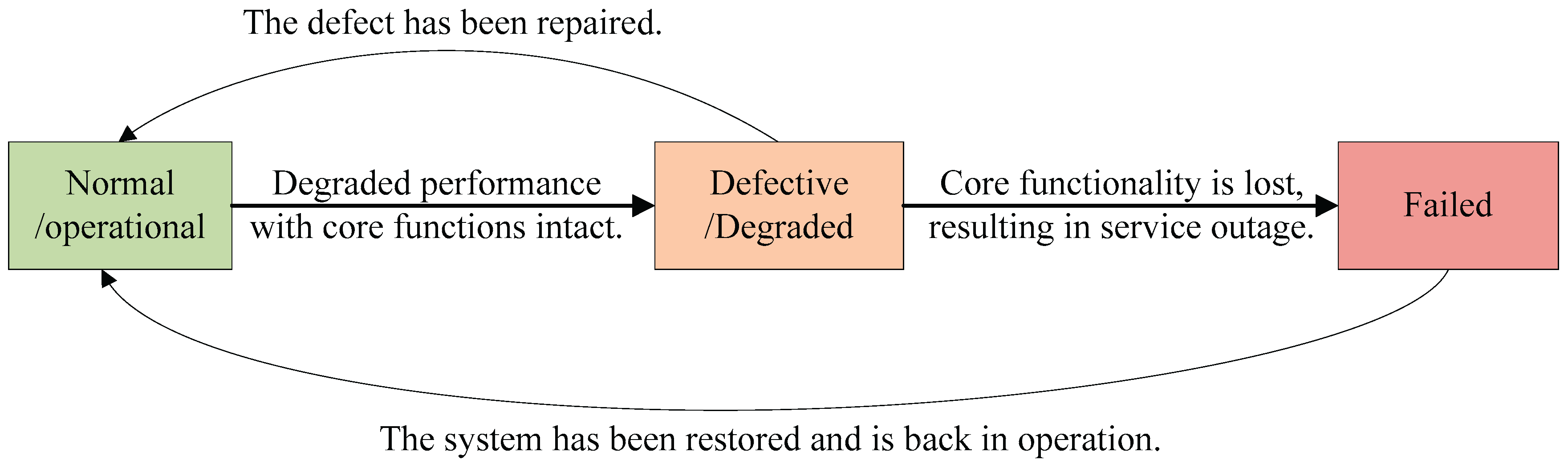
Figure 2.
Schematic diagram of external shocks.
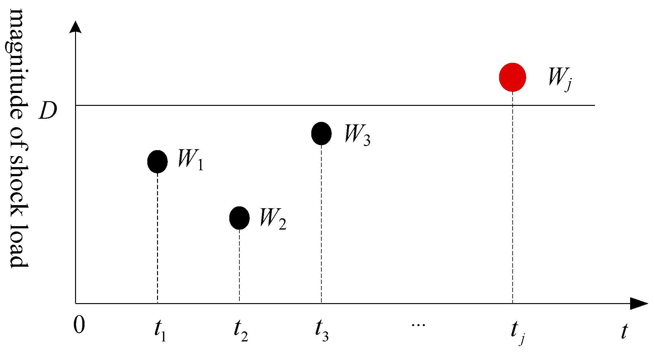
Figure 3.
Impact of imperfect repairs on the intensity function .
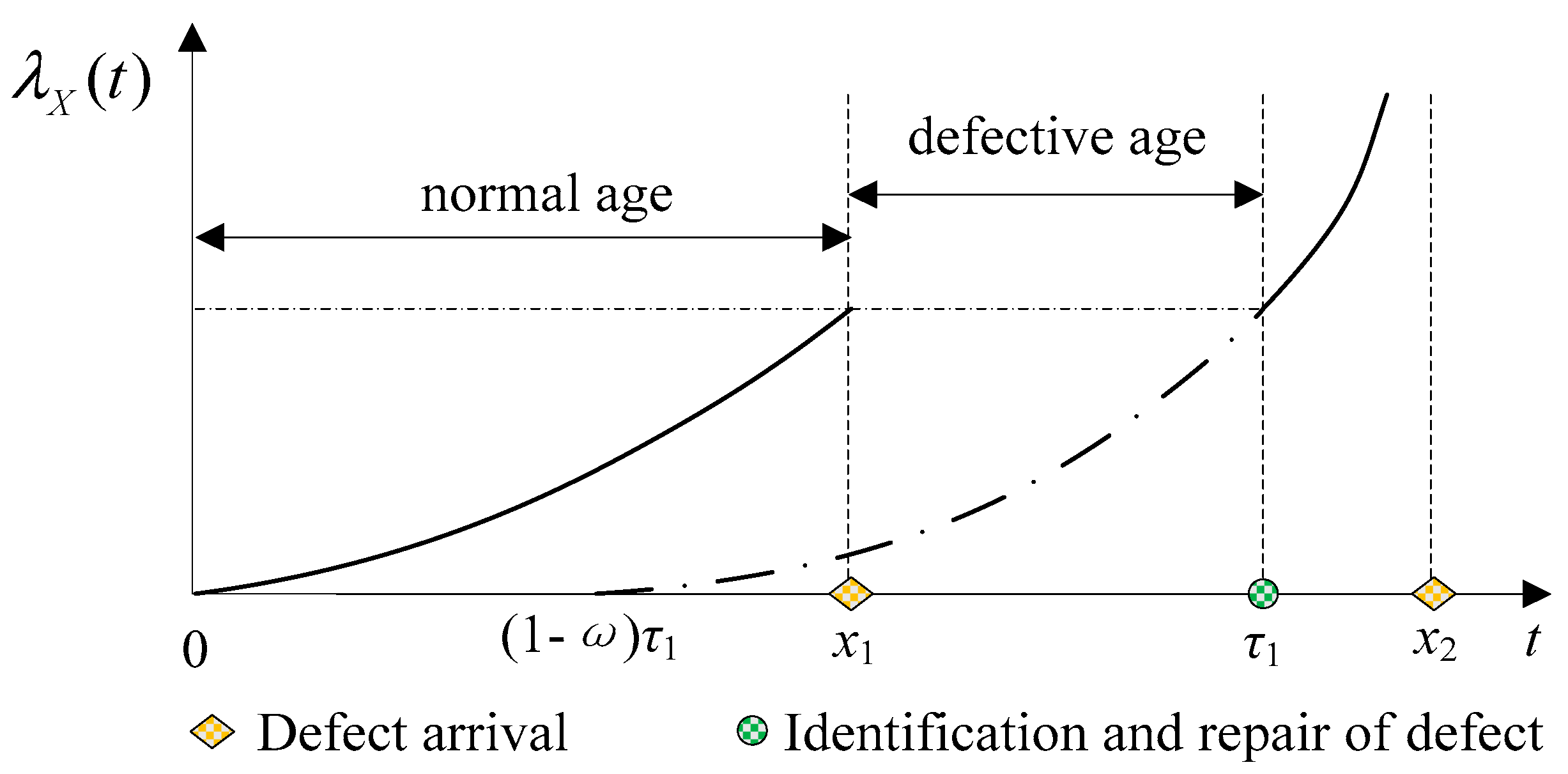
Figure 5.
Evolution pattern of system state in Case 2.
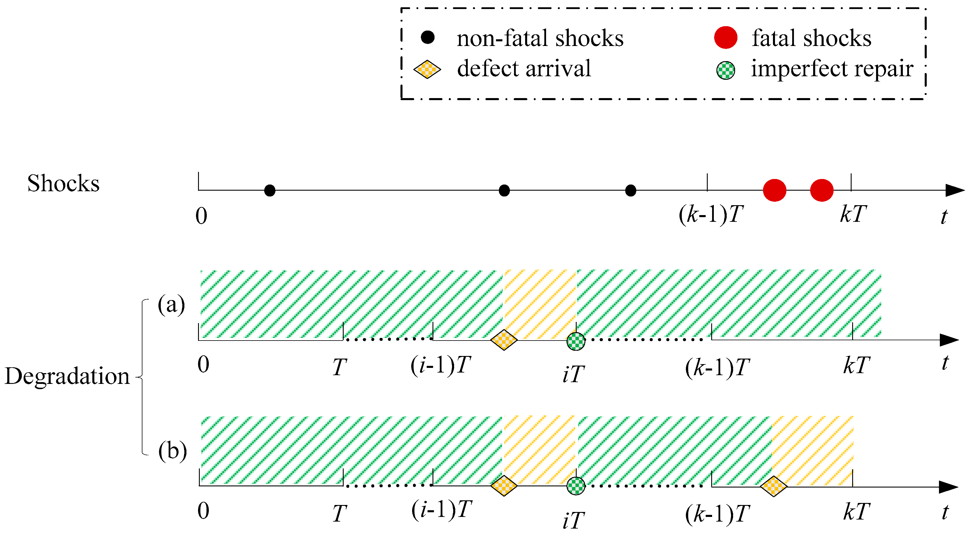
Figure 6.
Evolution pattern of system state in Case 3.
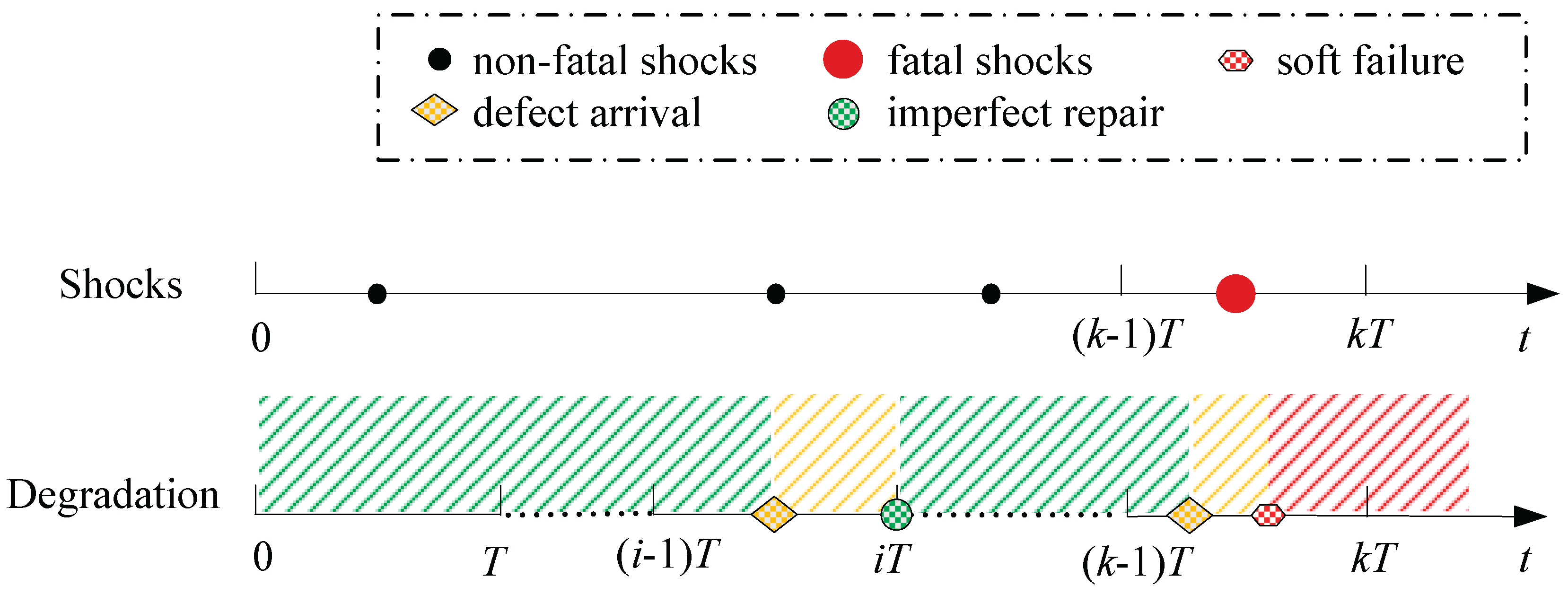
Figure 8.
Simulation flow chart.
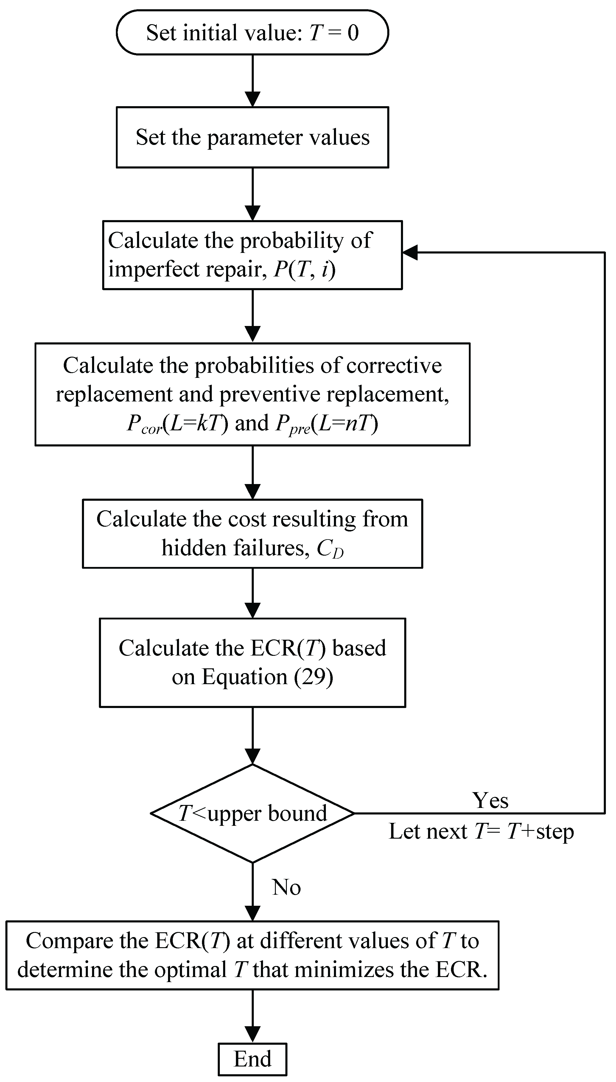
Figure 9.
Expected cost rate at different inspection intervals.
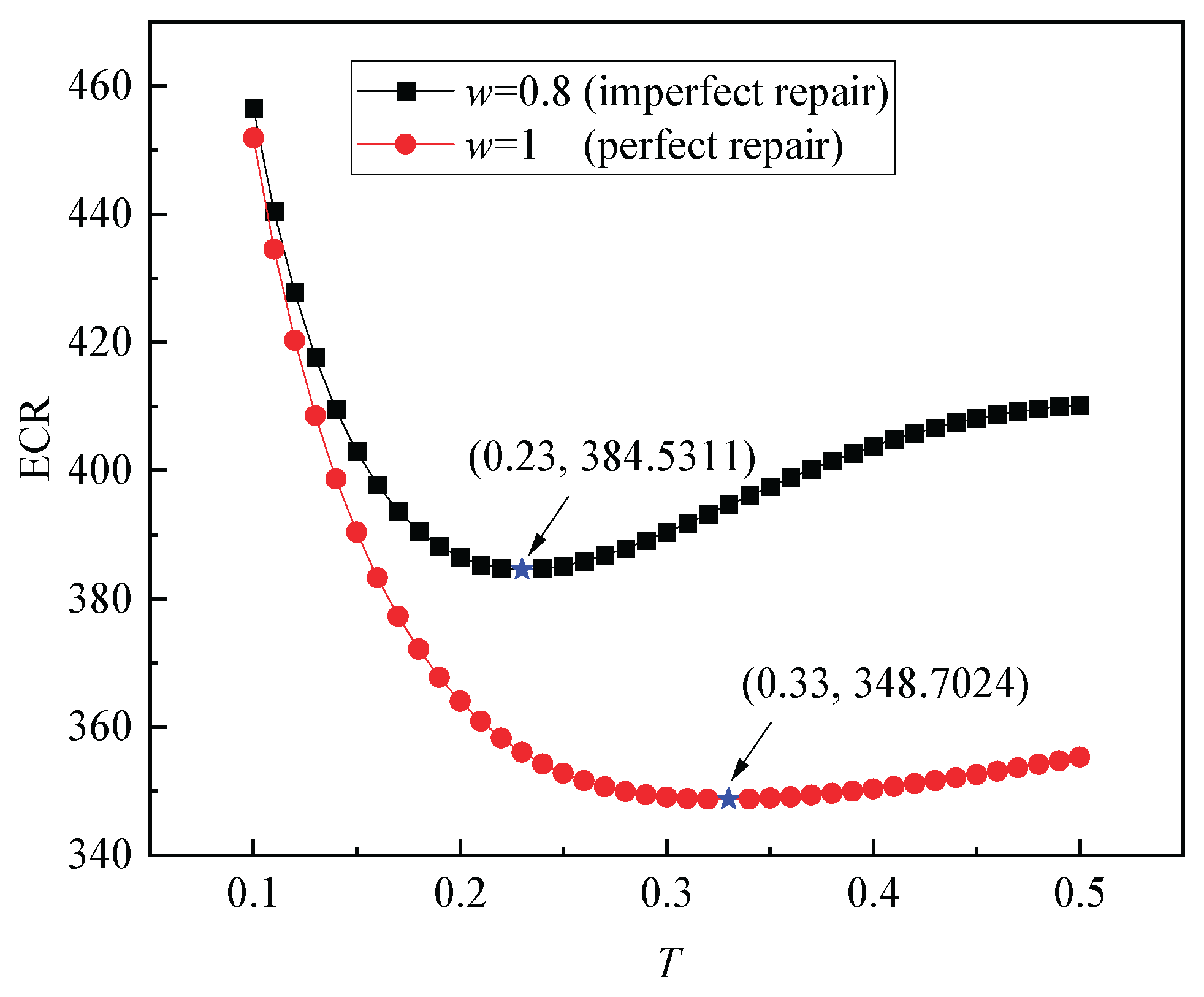
Figure 10.
Sensitivity analysis of the improvement factor ω.
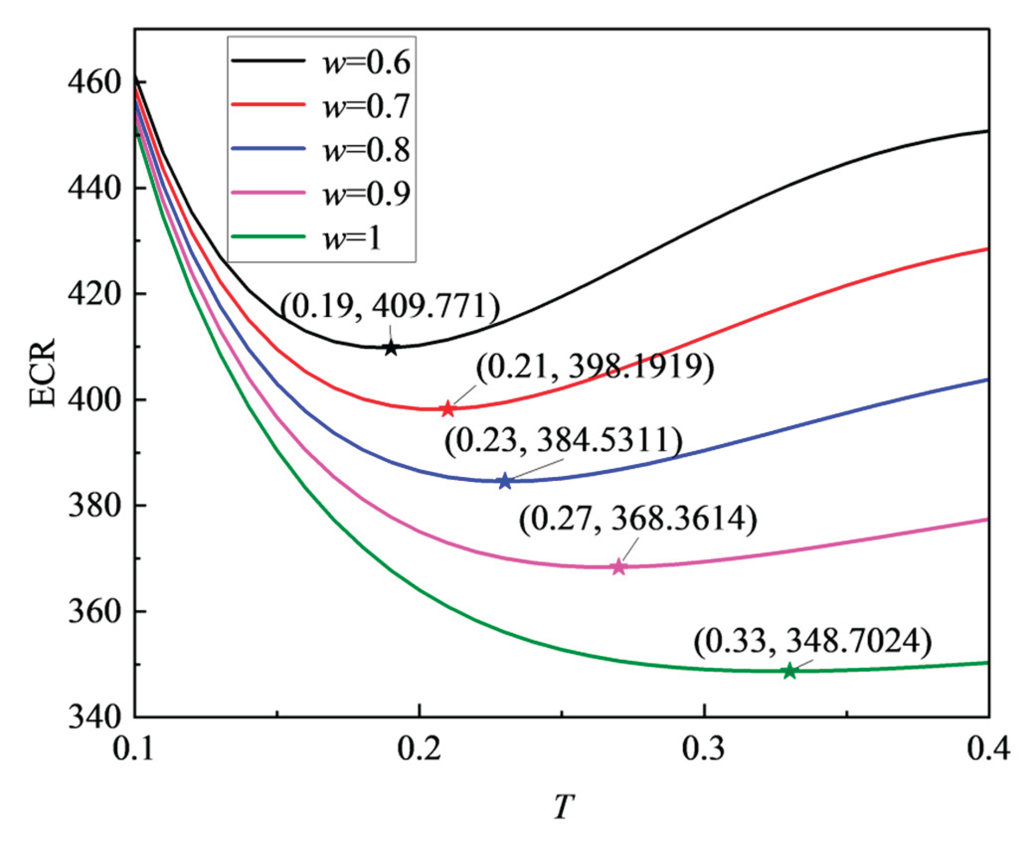
Figure 11.
Sensitivities of ECR(T*) (×$100) and T* to CI, CR, and CP.
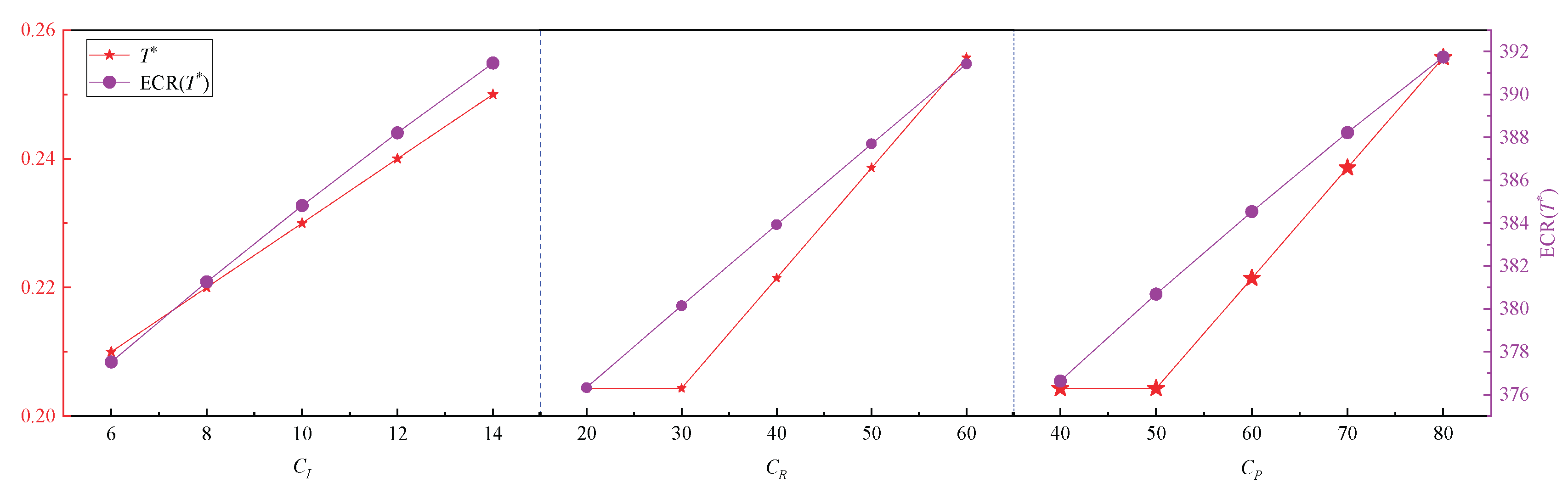
Figure 12.
Sensitivities of ECR(T*) (×$100) and T* to CC and Cd.
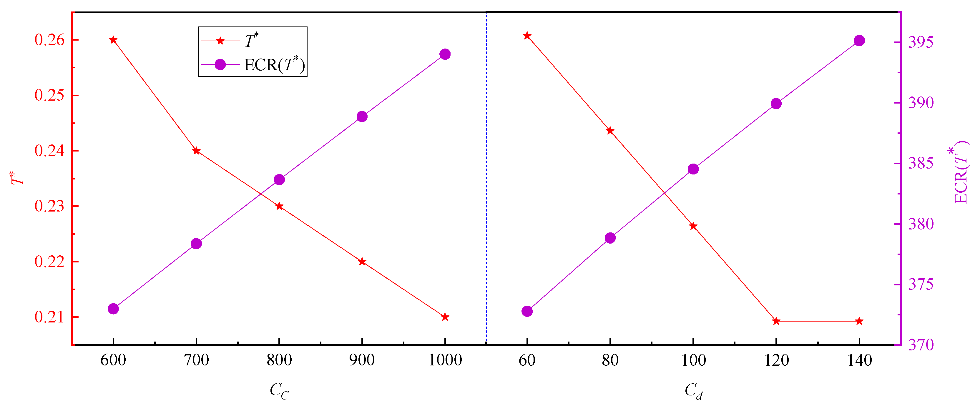
Figure 13.
Sensitivity of ECR(T*) (×$100) and T* to a uniform percentage change in cost parameters.
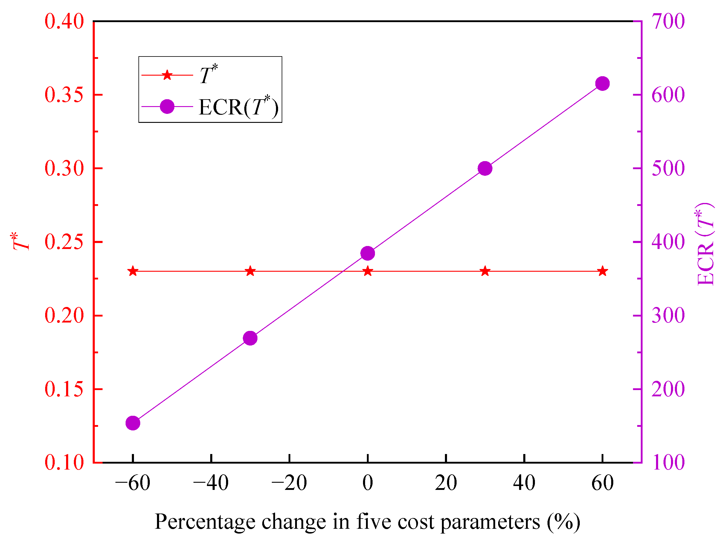

Table 1.
Optimal solutions under different cost parameters.
| Cost parameter | T* | ECR(T*) | ||||
| CI | CR | CP | CC | Cd | ||
| 6 | 40 | 60 | 800 | 100 | 0.21 | 366.3166 |
| 8 | 40 | 60 | 800 | 100 | 0.22 | 375.6450 |
| 10 | 40 | 60 | 800 | 100 | 0.23 | 384.5311 |
| 12 | 40 | 60 | 800 | 100 | 0.24 | 393.0203 |
| 14 | 40 | 60 | 800 | 100 | 0.25 | 401.1472 |
| 10 | 20 | 60 | 800 | 100 | 0.22 | 338.0560 |
| 10 | 30 | 60 | 800 | 100 | 0.22 | 361.3959 |
| 10 | 40 | 60 | 800 | 100 | 0.23 | 384.5311 |
| 10 | 50 | 60 | 800 | 100 | 0.24 | 407.5389 |
| 10 | 60 | 60 | 800 | 100 | 0.25 | 430.3200 |
| 10 | 40 | 40 | 800 | 100 | 0.22 | 376.6323 |
| 10 | 40 | 50 | 800 | 100 | 0.22 | 380.6841 |
| 10 | 40 | 60 | 800 | 100 | 0.23 | 384.5311 |
| 10 | 40 | 70 | 800 | 100 | 0.24 | 388.2153 |
| 10 | 40 | 80 | 800 | 100 | 0.25 | 391.7374 |
| 10 | 40 | 60 | 600 | 100 | 0.26 | 334.0888 |
| 10 | 40 | 60 | 700 | 100 | 0.24 | 359.5363 |
| 10 | 40 | 60 | 800 | 100 | 0.23 | 384.5311 |
| 10 | 40 | 60 | 900 | 100 | 0.22 | 409.1874 |
| 10 | 40 | 60 | 1000 | 100 | 0.21 | 433.6087 |
| 10 | 40 | 60 | 800 | 60 | 0.25 | 372.7835 |
| 10 | 40 | 60 | 800 | 80 | 0.24 | 378.8396 |
| 10 | 40 | 60 | 800 | 100 | 0.23 | 384.5311 |
| 10 | 40 | 60 | 800 | 120 | 0.22 | 389.9357 |
| 10 | 40 | 60 | 800 | 140 | 0.22 | 395.1355 |
Table 2.
Adjusted value of each cost parameter (in $100 units) after a uniform change of .
| Number | Percentage change | CI | CR | CP | CC | Cd | T* | ECR(T*) |
| 1 | -60% | 4 | 16 | 24 | 320 | 40 | 0.23 | 153.8124 |
| 2 | -30% | 7 | 28 | 42 | 560 | 70 | 0.23 | 269.1717 |
| 3 | 0% | 10 | 40 | 60 | 800 | 100 | 0.23 | 384.5311 |
| 4 | +30% | 13 | 52 | 78 | 1040 | 130 | 0.23 | 499.8904 |
| 5 | +60% | 16 | 64 | 96 | 1280 | 160 | 0.23 | 615.2497 |
Disclaimer/Publisher’s Note: The statements, opinions and data contained in all publications are solely those of the individual author(s) and contributor(s) and not of MDPI and/or the editor(s). MDPI and/or the editor(s) disclaim responsibility for any injury to people or property resulting from any ideas, methods, instructions or products referred to in the content. |
© 2025 by the authors. Licensee MDPI, Basel, Switzerland. This article is an open access article distributed under the terms and conditions of the Creative Commons Attribution (CC BY) license (http://creativecommons.org/licenses/by/4.0/).
Copyright: This open access article is published under a Creative Commons CC BY 4.0 license, which permit the free download, distribution, and reuse, provided that the author and preprint are cited in any reuse.


