Submitted:
10 September 2025
Posted:
11 September 2025
You are already at the latest version
Abstract
Radiative transfer models (RTMs) are foundational to optical remote sensing for simulating vegetation and atmospheric properties. However, their significant computational cost, especially for 3D RTMs and large-scale applications, severely limits their utility. Emulation, or surrogate modeling, has emerged as a highly effective strategy, accurately and efficiently replicating RTM outputs. This review comprehensively surveys recent developments in emulating vegetation and atmospheric RTMs. We discuss the methodological underpinnings, including suitable machine learning regression algorithms, effective training sampling strategies (e.g., Latin Hypercube Sampling, active learning), and spectral dimensionality reduction methods (e.g., PCA, autoencoders). We then synthesize key emulation applications such as global sensitivity analysis, synthetic scene generation, scene-to-scene translation (e.g., multispectral-to-hyperspectral), and retrieval of geophysical variables using remote sensing data. The paper concludes by outlining persistent challenges in generalizability, interpretability, and scalability, while also proposing future research avenues: investigating advanced deep learning algorithms (e.g., physics-informed and explainable architectures), developing multimodal/multitemporal frameworks, and establishing community benchmarks, tools and libraries. Emulation ultimately empowers remote sensing workflows with unparalleled scalability, transforming previously unmanageable tasks into viable solutions for operational Earth observation applications.
Keywords:
emulation
; radiative transfer models
; machine learning
; vegetation
; atmosphere
; surrogate modeling
; global sensitivity analysis
; scene generation
1. Introduction
In optical remote sensing, radiative transfer models (RTMs) are fundamental physical tools. They describe the complex interactions of electromagnetic radiation with Earth’s surface and atmosphere, providing a theoretical framework for understanding observed signals [e.g., [1,2,3]]. Specifically, vegetation RTMs simulate light interactions within plant canopies to characterize biophysical properties [4], while atmospheric RTMs describe how radiation is modified by atmospheric constituents, enabling atmospheric correction and sensor signal interpretation [5]. These models collectively serve as the theoretical backbone for understanding and interpreting the complex interactions between radiation and the Earth’s surface and atmosphere, and are essential for generating synthetic observations and designing robust retrieval algorithms [6]. The most commonly used RTM for vegetation is PROSAIL [7,8], which simulates leaf and canopy reflectance as a function of biophysical variables such as leaf area index (LAI) and chlorophyll content [9,10]. Based on the principles of PROSAIL, the energy balance model SCOPE (Soil Canopy Observation, Photosynthesis and Energy balance) [11] extends this approach by additionally modeling energy fluxes and solar-induced chlorophyll fluorescence (SIF) [12]. Both RTMs represent vegetation as a turbid medium, i.e., a one-dimensional (1D) representation of a canopy, which simplifies canopy architecture. In recent years, more structurally explicit 3D RTMs have gained traction, such as DART (Discrete Anisotropic Radiative Transfer) [13] and LESS (LargE-Scale remote sensing data and image Simulation framework) [14], which account for detailed canopy structure and enable more realistic scene simulations. These models have likewise evolved in simulating multiple types of radiation, such as SIF and laser scanning [15,16]. This increase in realism, however, comes at the cost of significantly higher computational demands, often resulting in long rendering times for a single simulation. RTMs also play a key role in accounting for atmospheric effects on solar radiation in remote sensing applications. The 6S model (Second Simulation of a Satellite Signal in the Solar Spectrum) [17] and MODTRAN (MODerate resolution atmospheric TRANsmission) [18] are two of the most frequently employed RTMs for simulating atmospheric transmittance, path radiance, and surface-atmosphere interactions. Similar to MODTRAN, libRadtran (library for radiative transfer.) [19] offers a flexible and high-accuracy radiative transfer framework that supports spectral calculations in both the solar and thermal domains, allowing for detailed simulation of various atmospheric scenarios, including aerosols, clouds, and surface reflectance anisotropy. These models are essential for atmospheric correction of satellite observations and retrieval of surface reflectance [20].
Despite their inherent strengths, RTMs—particularly structurally explicit 3D canopy models—incur substantial computational demands. This limitation becomes especially pronounced when applied in large-scale or iterative frameworks such as global mapping, operational biophysical retrieval, uncertainty quantification, or data assimilation. Depending on the model’s complexity, a single RTM simulation can range from milliseconds (e.g., PROSAIL) to several minutes or even hours (e.g., 3D DART or LESS simulations). Atmospheric RTMs (e.g., 6S, MODTRAN, libRadtran) exhibit similar challenges: their high dimensionality and detailed parameterizations make them computationally intensive, particularly in applications involving inversion, time-series reconstruction, or coupled canopy-atmosphere modeling [20]. While individually relatively fast, the necessity to execute these RTMs hundreds of thousands or even millions of times across vast parameter spaces, entire satellite images (e.g., millions of pixels), or long time series renders them impractical for real-time or near-real-time scenarios. These computational demands often stem from the complex physical equations and iterative numerical solutions required to simulate light interactions, especially across high-dimensional input spaces and spectral ranges [21].
To address these limitations, over the past two decades emulation has emerged as a promising strategy [22]. Emulation, also known as surrogate modeling, involves constructing a simplified, computationally inexpensive statistical model (an emulator or surrogate model) that accurately approximates the input-output relationship of a more complex, computationally demanding model or data transformation [23]. This is typically achieved by capitalizing on statistical learning techniques to train the emulator on a limited, yet carefully selected, set of simulations (i.e., from a physical model) or empirical observations (i.e., from data) [24,25]. Once trained, these emulators provide predictions orders of magnitude faster, frequently completing computations in microseconds, while preserving high accuracy. This drastic speed-up transforms previously intractable problems into feasible ones, opening new avenues for research and operational applications, such as in optical remote sensing science [e.g., [26,27]].
Since their introduction in remote sensing science and driven by advancements in statistical learning, we are witnessing the rapid emergence of emulators, with applications expanding across multiple domains in Earth observation (EO). In an attempt to grasp recent developments and anticipate future directions, this review examines how emulation contributes to the growing effectiveness of RTMs and remote sensing workflows, especially in vegetation and atmospheric EO studies. By reviewing and synthesizing recent scientific literature, we highlight key methodological advances in emulation, such as the selection of suitable machine learning regression algorithms (MLRAs) and efficient sampling strategies, alongside emerging image processing applications, including sensitivity analysis, synthetic scene generation, image-to-image transformations, and retrieval applications. We close with outlining promising directions for future research in this rapidly evolving field.
2. The Challenge of Computationally Expensive RTMs in EO Applications
Vegetation RTMs are essential for interpreting remote sensing data by simulating light interaction with plant canopies, with complexity varying across models [3]. PROSAIL, a combination of PROSPECT and SAIL, serves as a benchmark RTM due to its moderate complexity and widespread use [9,10]. PROSAIL couples leaf-level optical properties with a turbid medium representation of the canopy. Building upon this model, SCOPE represents a significant upgrade, integrating radiative transfer with detailed biophysical processes, e.g., photosynthesis and the full energy budget, while still relying on turbid medium principles [11,12]. At the highest level of complexity, we find RTMs that use discrete ordinate methods or ray tracing to explicitly simulate photon paths through detailed, heterogeneous 3D scenes. These models, such as DART, precisely account for all orders of scattering, clumping, and shadowing, offering a physically rigorous representation of radiative transfer [13,15,16]. Similarly, to seek a physical and realistic radiative transfer over heterogeneous scenes, LESS uses Monte Carlo (MC) ray tracing to simulate photon interactions within highly detailed 3D vegetation canopies [14], often reconstructed from LiDAR data [28]. Designed for scalability, LESS emphasizes computational efficiency while retaining realism in canopy architecture and light transport by using a lightweight boundary-based leaf cluster description approach [29] or semi-empirical-based radiative transfer acceleration technique [30], making it especially suited for simulating remote sensing signals, including images, LiDAR point clouds, and SIF, over large forested or agricultural landscapes.
While powerful, on the downside, these advanced RTMs impose significant computational bottlenecks in high-throughput tasks such as pixel-wise inversion over satellite scenes or global sensitivity analyses. For instance, a typical 10-meter resolution Sentinel-2 (S2) image covering 100x100 km contains pixels. Performing a full RTM inversion for each pixel, which might involve iterative optimization or look-up table (LUT) searches, would be computationally burdensome for operational product generation, potentially taking days or even weeks. This challenge is further compounded when considering time series analysis, where the same pixels need to be processed across many dates.

Table 1.
Overview of representative RTMs in vegetation and atmosphere domains. refs: references.
| Canopy RTMs | |||
|---|---|---|---|
| Model | Key Features | Outputs | Key refs. |
| PROSAIL | Leaf and canopy optics | Reflectance | [7,8,9,10] |
| SCOPE | Energy balance, photochemistry | Reflectance, SIF, fluxes | [11,12,31,32] |
| FLIGHT | 3D canopy architecture, detailed scattering | Reflectance, SIF | [33,34] |
| DART | 3D voxel, facet and ray tracing, heterogeneous scenes | Reflectance, radiance, LiDAR, SIF | [13,15,16,35] |
| LESS | 3D voxel, facet and ray tracing, heterogeneous scenes | Reflectance, SIF, LiDAR, fluxes | [14,29,36] |
| Atmosphere RTMs | |||
| 6S | Atmospheric correction, TOA reflectance | TOA radiance, transmittance | [17,37] |
| MODTRAN | Spectral transmission, path radiance | Radiative transfer profiles | [18,38] |
| libRadtran | Line-by-line, multiple scattering, trace gases | High spectral resolution radiance | [19,39] |
Introducing atmospheric RTMs (e.g., 6S, MODTRAN, libRadtran), adds yet another layer of complexity. Atmospheric RTMs simulate how radiation is modified by atmospheric gases (e.g., water vapor, ozone), aerosols (e.g., type, optical depth), and viewing geometry (solar and observation angles). These models are essential for atmospheric correction, converting top-of-atmosphere (TOA) radiance to surface reflectance. When subsequently coupling these atmospheric RTMs with vegetation RTMs, e.g., to simulate TOA reflectance from surface properties and atmospheric conditions for sensor design or retrieval algorithm training at the TOA scale, the resulting simulation chains become even slower and higher-dimensional. The interaction of numerous input parameters, such as varying aerosol loads, water vapor content, and viewing geometries, can easily result in parameter spaces spanning tens of dimensions [20].
Consequently, traditional inversion methods based on brute-force iterative optimization methods (e.g., downhill simplex, Levenberg-Marquardt) become impractical at scale [e.g., [40,41]], while limiting the size of LUTs to enhance processing speed typically leads to a decline in retrieval accuracy [42]. Even advanced MC sampling methods, commonly used for uncertainty quantification (UQ), normally demand thousands to millions of model runs, rendering them unfeasible for large-scale applications without substantial computational resources [43]. These inherent challenges underscore the critical need for fast emulators that can accurately and efficiently approximate RTM outputs across these vast and complex domains.
3. Emulation as a Surrogate Modeling Strategy
3.1. General Principles and Core Emulation Approaches
The principle of emulation entails constructing a computationally efficient surrogate model that approximates the behavior of a complex RTM or other deterministic, physically-based models [22]. For several decades, statistical learning techniques have been employed in climate and environmental sciences to emulate complex system dynamics [e.g., [24,44,45,46,47,48,49,50,51]]. In remote sensing, emulation functions as an inverse regression model. While a typical regression model uses spectral data to predict vegetation or atmospheric properties, emulation instead takes atmospheric or biophysical RTM parameters as an input to generate synthetic spectral data. In the context of RTMs, these emulators aim to replicate RTM outputs with high accuracy while drastically reducing computation time—often achieving speed-ups of several orders of magnitude [6,27]. See also Figure 1 for a visual illustration of the RTM emulation concept. This efficiency gain is especially advantageous in computationally intensive workflows, such as replicating outputs from advanced RTMs, model inversion, sensitivity analysis, data assimilation, and operational near-real-time applications.
A common characteristic of these emulators is their foundation in adaptive and flexible MLRAs [22,52]. MLRAs enable the modeling of non-linear relationships between input and output parameters. Owing to their relatively low computational cost, these algorithms allow emulators to generate spectral outputs far more rapidly than running full RTMs. Emulators are typically trained on a representative set of RTM simulations, which span the range of relevant input parameters. Once trained, they can rapidly predict outputs for unseen input combinations with negligible computational overhead. This enables the efficient exploration of high-dimensional parameter spaces that would be prohibitively slow using the original RTMs [6,27]. Importantly, emulators are usually validated against the original RTM to ensure fidelity to physical laws, which enhances generalizability, especially when extrapolating slightly beyond the training domain [e.g., [26,27]].
Emulators are thus fundamentally built upon statistically learned models. Recent advances in MLRAs—and more recently in deep learning—have significantly enhanced the predictive capabilities and broadened the applications of emulators [53]. A wide range of emulation approaches has been employed to approximate RTMs efficiently, spanning from classical data-driven regression algorithms to the latest advanced MLRAs. MLRAs such as Neural Networks (NN) and, upcoming, deep learning NNs (DLNNs), Gaussian Process Regression (GPR), Random Forests (RF), Support Vector Regression (SVR), Kernel Ridge Regression (KRR), and Polynomial Chaos Expansion (PCE) have been successfully used to emulate various types of physically based models (see Table 2 and Table 3 for details). Although PCE has seen little use in RTM emulation, it is worth highlighting due to its established role in emulation studies in other fields [e.g., [54,55,56,57,58]]. The suitability of each method depends on factors including the RTM’s complexity and non-linearity, the dimensionality of the input space, interpretability needs, and whether uncertainty quantification (UQ) is required [52].
Table 2 summarizes the key characteristics, advantages, and limitations of established MLRAs used for RTM emulation. GPR remains a strong choice for its inherent UQ and effectiveness with small datasets, though its high computational cost hampers scalability. NNs and Deep Learning NNs (DLNNs) are well-suited for capturing complex, nonlinear relationships and scale efficiently to large datasets. DLNNs offer state-of-the-art performance in high-dimensional and data-rich scenarios, yet they require significant training data, are more opaque in their interpretability, and only provide approximate uncertainty estimates unless explicitly designed to do so. RFs are valued for their robustness, fast training, and interpretability via feature importance measures. Although RFs can approximate predictive uncertainty through ensemble variance, they lack a principled probabilistic UQ framework and may underperform on fine-grained, highly continuous outputs. SVR achieves high accuracy and robustness in medium-sized datasets, though it is sensitive to kernel and hyperparameter settings and struggles with large-scale datasets. KRR offers competitive accuracy with fewer tuning demands than GPR and SVR—and therefore trains faster and is more efficient in application—but lacks native uncertainty estimates. Finally, PCE excels in analytical UQ and global sensitivity analysis, but is constrained by the curse of dimensionality (yet, see also Section 4.2) and has limited flexibility in capturing strong nonlinearities. Overall, the selection of an emulation method depends on trade-offs between accuracy, scalability, interpretability, and the need for UQ, with different approaches better suited to different RTMs and application settings.
Two examples of GPR emulators are presented in Figure 2. GPR was selected as the emulator since it achieved the highest accuracy among the evaluated MLRAs when trained and validated on the original spectra (results not shown; illustrative purpose only). In comparison to the computational demands of the original simulations—requiring about half an hour to nearly a full day on a single CPU to generate (1) top-of-canopy (TOC) reflectance with LESS or (2) TOA radiance spectra with the coupled PROSAIL–libRadtran models—the GPR emulators reproduced, respectively, one thousand TOC reflectance and TOA radiance spectra within seconds. Training of each emulator was completed in under 20 seconds, underscoring the orders-of-magnitude computational savings.
3.2. Proof-of-Concept Studies Demonstrating the Potential of Emulation in Approximating RTMs
Initial proof-of-concept studies effectively illustrated the capability of emulators to replicate RTM outputs with high precision and notable computational efficiency. While emulation has a longer history in other scientific fields, its application to RTMs began around a decade ago with two pioneering works. First, Rivera et al. [26] introduced a statistical learning-based emulator toolbox for approximating SCOPE outputs—specifically reflectance and SIF. Among the evaluated MLRAs, KRR and NNs achieved high reconstruction accuracy, with relative errors below 0.5% when trained on a small set of 500 simulations. Using principal component analysis (PCA) for dimensionality reduction, NN and KRR emulators ran approximately 50× and 800× faster, respectively, than the original SCOPE model. In parallel, Gómez-Dans et al. [27] demonstrated emulation use cases for both vegetation (PROSAIL) and atmospheric (6S) RTMs. Their GPR emulators reproduced model outputs and finite-difference-based gradients accurately, achieving speed-ups between 10,000 and 50,000 times compared to the original models. These foundational studies spurred broader research in exploring distinct RTMs, MLRAs, and output variables. For instance, Verrelst et al. [61] systematically evaluated the impact of machine learning type, integration with dimensionality reduction, and LUT size. Their results showed that well-configured GPR and NN emulators could reconstruct SCOPE outputs with relative errors below 2% for reflectance and 4% for SIF, and about 250 times faster than SCOPE. Vicent et al. [42] subsequently benchmarked emulation against classical interpolation techniques using PROSAIL and MODTRAN using MLRA and dimensionality reduction combinations. Emulation consistently outperformed interpolation techniques in spectral reconstruction, with GPR achieving up to tenfold higher accuracy while maintaining competitive speed. Additionally, GPR, formulated within a Bayesian framework, inherently provides associated uncertainty estimates (UQ).
3.3. Recent Progress in Emulation in Vegetation and Atmospheric RTMs
In the meantime, MLRA-based emulation of vegetation RTMs matured as an effective strategy to accelerate inversion workflows and enable large-scale applications. For example, Shi et al. [63] applied multiple regression algorithms—RF, ANN, and SVR—to emulate a coupled soil–canopy–atmosphere RTM ACRM (Atmospheric Correction Reflectance Model) [81] and 6S, enabling accurate and efficient retrievals of vegetation biophysical variables from satellite data. Extending to 3D canopy structures, Makhloufi and Kallel [82] developed an ANN-based emulator of the DART model, integrated with a continuous MC inversion framework. Applied to S2 imagery, this approach significantly reduced computational burden while supporting uncertainty-aware retrievals. Alternatively, [30] proposed a semi-empirically accelerated approach to accurately simulate reflectance from 400 nm to 2500 nm using a few predefined soil, branch, and leaf optical properties based on the four-stream theory, which provides the potential to emulate only a few bands to replicate the full spectral range of LESS-like simulations between 400 and 2500 nm with an acceleration of more than 320 times. These three studies demonstrate the potential of emulators to support accurate, scalable, and efficient RTM applications in vegetation remote sensing. However, despite the growing importance of 3D and coupled RTMs, applications of surrogate modeling remain scarce. The niche use of dedicated emulators for 3D RTMs highlights an important research gap and a promising opportunity to advance robust emulation frameworks for complex vegetation RTMs. Yet, emulation efforts have advanced more substantially in atmospheric applications.
Recent advances in atmospheric RTM emulation have capitalized on MLRAs to significantly improve computational efficiency and flexibility. Fundamental work by Brodrick et al. [64] introduced a generalized NN emulator for radiative transfer in imaging spectroscopy, enabling flexible reflectance retrievals from complex scenes. Veerman et al. [83] developed an NN surrogate for the gas optics component of RRTMGP (Rapid Radiative Transfer Model for General circulation - Parallel), achieving near-original accuracy with a fourfold speed-up. In the Earth system modeling context, Belochitski and Krasnopolsky [84] demonstrated that emulated RT components could be integrated into hybrid general circulation models (GCMs) while maintaining stable long-term behavior. Ukkonen [67] systematically explored design choices for neural RTM emulators, showing that architecture, input representation, and training strategies have a strong impact on emulation accuracy. Vicent Servera et al. [85] proposed a multifidelity GPR framework for emulating atmospheric RTMs, which integrates information from different fidelity levels to improve predictive performance and reduce training costs. Zhong et al. [86] applied an emulated RRTMG within the WRF (Weather Research and Forecasting) model, demonstrating notable runtime reductions without degrading forecast performance. Jasso-Garduño et al. [70] presented a DLNN emulator for the 6S RTM, enabling fast approximations of atmospheric corrections. Emulation of MODTRAN-based TOA reflectance for MODIS channels using RF and NNs was conducted by Gonzalez et al. [87], yielding accurate and efficient surrogates. Similarly, Lamminpää et al. [88] employed GPR to replicate NASA’s OCO-2 forward model with instrument-level accuracy and orders-of-magnitude speed-ups. The use of physics-informed NNs (PINNs) (see also Section 4.3) to directly solve the radiative transfer equation was demonstrated by Zucker et al. [89], offering physically consistent and accurate approximations. Additionally, emulation has been applied to aerosol optics in E3SM (Energy Exascale Earth System Model) using randomly wired NNs [90], and probabilistic surrogates have been proposed for CRTM (Community Radiative Transfer Model) in support of satellite data assimilation [91]. Finally, Sgattoni et al. [92] presented an emulation approach for the FORUM (Far-infrared Outgoing Radiation Understanding and Monitoring) satellite mission, selected as ESA’s 9th Earth Explore mission, aiming to approximate the inverse retrieval of atmospheric properties from far-infrared spectra using simulated data and NNs. Altogether, these studies underscore the increasing maturity and breadth of atmospheric RTM emulation, establishing it as a powerful approach across remote sensing, forecasting, and climate modeling domains.
3.4. Trends in MLRAs for RTM Emulation Applications
In light of the above studies, we can now evaluate the suitability of established MLRAs for emulation. Table 3 qualitatively compares commonly used MLRAs for RTM emulation based on four key characteristics: (1) accuracy—how well the emulator replicates RTM outputs; (2) uncertainty quantification (UQ)—the ability to estimate prediction confidence; (3) scalability—how efficiently the method handles increasing data size or complexity; and (4) interpretability—how transparently model behavior and predictions can be understood. Both standard NNs and DLNNs offer high accuracy and scalability, with DLNNs particularly suited for learning complex input–output mappings; yet, they are limited in interpretability and only provide approximate UQ. GPR excels in terms of UQ and accuracy, although scalability is limited. RF is robust and scalable, offers moderate-to-high accuracy, with empirical rather than intrinsic UQ. KRR and SVR offer balanced accuracy and interpretability, differing in scalability and UQ capabilities. KRR typically achieves superior emulation performance compared to SVR and offers better scalability with larger training datasets, thanks to the need to tune only a single regularization hyperparameter. PCE stands out for its analytical UQ and interpretability, making it ideal for sensitivity studies, albeit less suited to complex, high-dimensional problems. This likely explains why PCE is less suited for emulating RTM outputs, which often span hundreds of spectral bands. However, integrating PCE with dimensionality reduction techniques could help overcome this limitation (see Section 4.2). Selecting an appropriate MLRA requires balancing trade-offs among accuracy, UQ, scalability, and interpretability according to the application’s needs. In most emulator designs, accuracy is the primary driver, which often makes (DL)NNs the preferred choice. Conversely, when robust UQ is essential, GPR is often favored for its combination of high accuracy and intrinsic probabilistic framework, though its limited scalability constrains the feasible size of training datasets.
Emulation Applications Beyond RTMs: LSMs, ESMs, and DGVMs
While this review primarily addresses the emulation of RTMs in the optical domain, it is worth noting that emulation techniques have a long-standing history in other areas of Earth observation and environmental modeling. In fact, they have been widely used to accelerate computationally demanding environmental models for over a decade [e.g., [24,44,45,46,47,48,49,50,51]]. Recent emulation applications reflect the versatility of surrogate modeling in reducing computational costs, improving modeling and retrieval performance, and enabling large-scale analysis. Surrogate modeling has become instrumental in accelerating simulations and enabling uncertainty quantification in complex Earth system components, including Earth system models (ESMs), land surface models (LSMs), and dynamic global vegetation models (DGVMs). These large models often involve highly nonlinear, computationally intensive processes that simulate biogeophysical, hydrological, and biogeochemical dynamics across spatiotemporal scales.
Following this approach, Lu and Ricciuto [93] employed MLRA-based surrogates, including NNs and gradient boosted-decision trees (GBDTs), to emulate components of ESMs. In this context, dimensionality reduction techniques such as singular value decomposition (SVD) (see also Section 4.2) were applied to compress high-dimensional outputs before training the surrogate. Duffy et al. [94], Duffy et al. [95] proposed a general deep learning emulation framework for numerical models, demonstrating its applicability in satellite remote sensing and suggesting broader potential for Earth system and land surface model emulation. Regarding the domain of LSMs, Baker et al. [96] used sparse GPR (see also Section 4.3) to emulate outputs of the high-resolution JULES (Joint UK Land Environment Simulator) model. Their approach demonstrated that GPR can offer accurate surrogate representations even for fine-scale simulations at high speed, while enabling uncertainty estimation. Similarly, Xu et al. [97] used a GPR-based surrogate to support a Bayesian calibration framework for runoff-generation in E3SM, and Watson-Parris et al. [98] introduced ESEm (Earth System Emulator), an open and scalable emulator platform combining ensemble learning and dimensionality reduction for ESM calibration. Recent advancements extend emulation to complex processes like wildfire modeling and plant functional type dynamics. For example, Zhu et al. [99] developed a DLNN emulator for wildfire activities in ESMs using a fully connected NN, whereas Li et al. [100] applied XGBoost (see also Section 4.3) to emulate plant coexistence dynamics in the ELM-FATES model (a demographic vegetation model that operates within the E3SM land model framework (ELM)). At the climate system level, Beusch et al. [101], Beusch et al. [102] introduced MESMER (Modular Earth System Model Emulator with spatially Resolved output), a statistical framework to emulate temperature responses across spatial scales using a combination of pattern scaling and autoregressive modeling. Further, Bouabid et al. [103] proposed FaIRGP, a GP emulator for global surface temperature projections with uncertainty quantification. [104] also presented Graph Convolutional NNs (see also Section 4.3) as surrogate models for spatially explicit climate simulations with uncertainty quantification.
Overall, these examples highlight how MLRAs can serve as efficient, flexible surrogates for high-dimensional Earth system processes. When outputs are spectrally or spatially structured, dimensionality reduction using SVD or PCA is often employed to enhance learning efficiency and reduce emulator complexity.
4. Trends and Advances in Emulation Methodologies
4.1. Empirical vs RTM-Based Emulation: The Role of Training Data Sampling
One key distinction among emulators lies in the nature of their training inputs. Some emulators are trained on purely empirical relationships between inputs and observed spectral data, essentially learning directly from real-world data, e.g., for scene-to-scene translation (see also Section 5.3). However, the most robust approaches train emulators on simulated outputs from RTMs. This latter approach offers several critical advantages: it ensures consistency with known physical principles, allows for generalization across sensors and vegetation and atmosphere variability (as the underlying physics remains constant), and can even permit extrapolation to conditions not yet observed in real data. The capability to accurately replicate RTM’s output is crucial for broad applicability and predictive power in novel environments. To reach high output accuracy, the quality and representativeness of an emulator’s training data are paramount.
To train RTM emulators effectively, it is crucial to use efficient sampling strategies that comprehensively explore the high-dimensional input space and provide the model with a diverse set of training data. Ideally, the entire parameter space is sampled, including boundaries and rare combinations. To achieve so, space-filling sampling designs such as (1) Latin Hypercube Sampling (LHS) [105], (2) Sobol sequences [106], or (3) Halton sequences [107] are commonly employed. See Table 4 for a qualitative comparison of their key properties. These methods ensure that samples are uniformly spread across the entire input domain, thereby avoiding clustering and guaranteeing adequate coverage of all dimensions, which ultimately leads to better model generalization. For instance, LHS ensures that each dimension of the input space is sampled exactly once for each stratum, providing more uniform coverage than simple random sampling. Given its simplicity, flexibility, and ability to ensure well-distributed samples across high-dimensional input spaces, LHS has become the most widely adopted sampling strategy in RTM emulation studies [e.g., [26,42,61]]. LHS ensures that each parameter range is sampled evenly, making it markedly effective for generating training datasets from high-dimensional RTMs.
Alternatively, active learning and adaptive sampling techniques have emerged to further optimize the training process. Instead of pre-generating all training samples, these methods iteratively select new samples based on the current emulator’s uncertainty. For example, measures of Euclidean-based diversity (see review for regression applications: [108]) or regions of high predictive variance can guide the sampling process. This allows focusing sampling efforts on areas where the model is least confident or where the RTM response exhibits high nonlinearity. For instance, Ma et al. [72] explored the active subspace method [109] finds a low-dimensional linear subspace (spanned by combinations of input variables) that captures most of the important variation in the output. Another notable implementation of this principle is the AMOGAPE (Active Multi-Output Gaussian Process Emulator) framework, introduced by Svendsen et al. [110], which combines GPR-based emulation with an active sampling strategy tailored for RTM’s spectral outputs. The acquisition function balances exploration and exploitation by targeting inputs that yield high predictive uncertainty or rapid output variation. Their results demonstrated that this strategy can substantially reduce the number of RTM evaluations needed to construct accurate emulators, especially in complex or high-dimensional settings. Although AMOGAPE is built upon GPR, overall, active learning and adaptive sampling techniques can offer a promising direction for building efficient surrogate models.
4.2. The Role of Spectral Dimensionality Reduction in Emulation of RTMs
Spectral dimensionality reduction techniques are frequently applied in emulating the RTM spectral output space (e.g., reflectance, radiance, SIF) that can comprise hundreds of bands. Spectral data often exhibit high collinearity [111], which allows effective compression using dimensionality reduction methods such as: (1) PCA [112], (2) SVD [113], or (3) autoencoders [114]. These are the most common dimensionality reduction approaches in RTM emulation, particularly for compressing spectral data and large LUTs. See Table 5 for a qualitative comparison of these three methods on their key properties. PCA remains the most general dimensionality reduction method in RTM emulation studies, as autoencoders are integral to NN designs. SVD is sometimes used in emulation studies of environmental models (see Section 3.4). Although when applied to mean-centered data, both SVD and PCA yield identical principal component directions and projections [112,115]. The compression of spectral data reduces the computational burden for the emulator, as it learns to predict fewer dimensions, and can improve generalization by filtering out noise and focusing on the most dominant spectral features. Importantly, both PCA and autoencoders enable reconstruction of the full spectral domain using back-projection, i.e., the inverse transformation (for PCA) or the decoder network (for autoencoders), thereby allowing for emulation of the complete reflectance or radiance spectrum from the reduced representation. It is likewise possible for the input data to comprise spectral information, as opposed to the traditional RTM input parameters. In such cases, dimensionality reduction techniques can be likewise applied to both input and output spaces, accompanied by a reconstruction step (see also Section 4.2). Likewise, although less commonly encountered in emulation studies, another potentially promising dimensionality reduction technique would be functional PCA (FPCA) [109], which is a variant of PCA. FPCA is specifically designed for functional data. Functional data are observations that are themselves functions or curves, rather than discrete, fixed-dimensional vectors. These functions are typically observed over a continuous domain (e.g., wavelength) [116]. Also note that other common dimensionality reduction methods such as t-SNE [117], Isomap [118], UMAP [119], and Kernel PCA [120] do not enable back-projection, which makes spectral reconstruction difficult; back-projection typically would require training a separate inverse model.
example
4.3. Advanced Machine Learning for Emulation
Whereas the above sections demonstrated that established MLRAs are already used in the emulation of vegetation and atmosphere RTMs, several more novel algorithms—though not yet widely adopted in RTM applications—hold promise for developing more scalable, accurate, and uncertainty-aware surrogate models. These include scalable variants of GPR, deep learning architectures (e.g., CNNs, transformers, GANs), and advanced gradient decision-tree ensembles (e.g., XGBoost, LightGBM, CatBoost). Bayesian methods such as BART and Bayesian NNs (BNNs) offer native uncertainty quantification. Table 6 summarizes the most relevant methods, their main strengths, and associated references. These emerging approaches could serve as a foundation for future developments in RTM emulation workflows. Recent studies outside the strict RTM domain already illustrate the potential of these advanced methods. Sparse GPR has been used to emulate high-resolution outputs of the JULES land surface model [96]. XGBoost has been applied to emulate plant coexistence dynamics in the ELM-FATES demographic vegetation model within the E3SM framework [100]. Graph Convolutional NNs (GCNNs) have been proposed as surrogate models for spatially explicit climate simulations with integrated uncertainty quantification [104]. More recently, physics-informed NNs (PINNs) have been employed to directly solve the radiative transfer equation, enabling physically consistent and accurate approximations [89]. In the context of RTM emulation, choosing a suitable advanced MLRA would depend on factors such as the size and dimensionality of RTM outputs (although the methods could be combined with dimensionality reduction), the availability of training data, the need for interpretability or uncertainty estimates, and computational constraints.
5. Applications of Emulation
Having introduced the principles of emulators in optical remote sensing, we now turn to their practical applications. In RTM emulation, an MLRA is trained on RTM simulations, with RTM input variables serving as predictors and RTM spectra as the outputs. Because spectral outputs are inherently high-dimensional, dimensionality reduction is typically applied; training the emulator on compressed spectral components, which are later reconstructed back into full spectra. This approach enables efficient, accurate surrogates for complex RTMs. In the following sections, we discuss four key application domains: (1) global sensitivity analysis, (2) synthetic scene generation, (3) scene-to-scene emulation, and (4) retrieval.
5.1. Emulation for Global Sensitivity Analysis of RTMs
Global Sensitivity Analysis (GSA) quantifies how much variation in an RTM’s output is attributable to each input parameter, including their interactions. Variance-based methods such as Sobol’s sensitivity indices (i.e., first-order and total Sobol indices) provide a comprehensive decomposition of output variance but traditionally require thousands to millions of costly RTM runs, making GSA practically infeasible for complex models [135]. Emulators can substantially alleviate this computational bottleneck by replacing the full RTM with a fast surrogate, enabling variance-based GSA to be performed in minutes or hours instead of weeks. This acceleration allows researchers to: (1) identify influential RTM input parameters such as LAI, chlorophyll content, soil brightness, or atmospheric variables like aerosol optical depth and water vapor; (2) reveal complex nonlinear interactions between parameters—e.g., the synergistic effect of chlorophyll and LAI on reflectance; and (3) optimize input parameter ranges to ensure efficient and representative simulation campaigns.
As a first demonstration of using emulators for GSA, Verrelst et al. [60] applied GPR, NN, and KRR emulators to the PROSAIL and MODTRAN5 models (see also Figure 3). Their work demonstrated the high accuracy of the emulators, and then successfully identified the key drivers of spectral variability. Extending this work, Verrelst et al. [136] performed a detailed emulator-based GSA on a coupled leaf-canopy-atmosphere RTM system (PROSAIL + MODTRAN5). Their GPR emulator achieved high fidelity (<2.5% relative error), allowing the identification of dominant contributors to TOA radiance. Results revealed that vegetation parameters (e.g., leaf chlorophyll, water thickness, LAI) dominated over atmospheric ones, demonstrating the feasibility of direct biophysical retrieval from TOA data without prior atmospheric correction. Similarly, in the atmospheric domain, Vicent Servera et al. [85] proposed a multifidelity GPR emulator framework for MODTRAN to support GSA while balancing computational cost and accuracy. Progressing along this line, Vicent Servera et al. [137] subsequently introduced a physics-aware feature selection framework for RTM emulation. By aligning GPR feature selection with variance-based GSA, the method pinpointed key atmospheric variables such as solar zenith angle, water vapor, and aerosol properties, contributing to more interpretable emulation pipelines. In the context of operational atmospheric correction, Zhou et al. [138] used MODTRAN and libRadtran to build LUTs, which were then emulated using an RF model to enable rapid GSA and subsequent surface reflectance estimation. Their GSA highlighted visibility and water vapor as dominant parameters affecting surface reflectance. It was concluded that emulator integration not only improved computational efficiency but also enhanced understanding of parameter sensitivity, supporting practical implementation in large-scale processing workflows. Overall, these works confirm that emulator-enabled GSA uplifts sensitivity analysis from a theoretical possibility into a practical and fast tool for RTM understanding, inversion optimization, and operational remote sensing retrieval model development.
5.2. RTM Emulation for Synthetic Scene Generation
RTM emulators also offer a fast alternative to generate synthetic reflectance or radiance scenes over simulated vegetated landscapes, vastly outperforming full RTM execution in speed. Importantly, emulated scenes can be tailored to specific sensor characteristics—such as spectral band configurations, signal-to-noise ratio, and spatial resolution—making them notably valuable within the context of satellite mission design. Those emulators can be subsequently integrated into end-to-end simulation frameworks [e.g., [139,140]] to assess system capabilities and optimize payload specifications. By emulating responses across large parameter spaces, emulators can form the core to enable fast exploration of "what-if" scenarios and foster a deeper understanding of how biophysical or environmental factors over a surface influence observed signals from space. This includes identifying sensitive spectral regions, investigating parameter interactions, or predicting sensor responses under unobserved conditions. In this context, a notable example is provided by Verrelst et al. [61], who developed GPR- and NN-based emulators of the SCOPE model to reproduce canopy reflectance and SIF spectra. Integrated into a so-called GUI Automated Scene Generator Module, the emulators produced synthetic sensor-specific reflectance and SIF images with <2% error for reflectance and <4% for SIF, thereby reducing processing time from days to minutes (see also Figure 4). These emulators support the simulation of realistic reflectance and SIF scenes over mapped landscapes and have been used in the context of ESA’s upcoming hyperspectral missions FLEX (FLuorescence EXplorer) [141] and CHIME (Copernicus Hyperspectral Imaging Mission) [142].
RTM-based emulators can also serve in spectral retrieval schemes that rely on physical principles. Pursuing this approach, Pato et al. [143] introduced a MODTRAN-based ML emulator that directly predicts at-sensor radiances in the O2-A absorption band, optimized for SIF retrieval. This emulator integrates physical radiative transfer principles embedded in MODTRAN with advanced learning using fourth-degree polynomial regression model to provide accurate and efficient estimates of radiance, facilitating improved SIF inversion from airborne or satellite hyperspectral sensor data. In summary, RTM-based emulators enable fast, scalable, and sensor-specific scene generation for EO application development, satellite mission design, and the processing of satellite imagery. Yet, aside from the studies mentioned above, their use for producing spatially explicit synthetic scenes remains largely unexplored, marking a clear opportunity for further research in end-to-end simulation frameworks and satellite image processing, e.g., in the context of developing atmospheric correction and retrieval pipelines [e.g., [85,138]].
5.3. Scene-to-Scene Emulation
Scene-to-scene emulation involves transforming spatially-explicit remote sensing products from one domain to another—for example, converting multispectral to hyperspectral reflectance, or airborne to satellite-scale SIF. This application is a higher-level form of emulation, distinct from traditional RTM emulators. Unlike RTM-based emulators, it leverages emulators trained on high-quality reference data to directly and efficiently map between image domains, enabling rapid generation of realistic, sensor-specific radiometric products. This process typically integrates dimensionality reduction at both input and output stages, with back-projection applied to reconstruct full-spectrum outputs.
Regarding the emulation of reflectance imagery, Verrelst et al. [136] presented a prototype of reflectance scene emulation in which S2 multispectral imagery was transformed into hyperspectral imagery using GPR models trained on empirical HyPlant hyperspectral reflectance observations. The resulting maps maintained physical consistency and spectral fidelity, enabling a first demonstration of hyperspectral scene reconstruction from operational satellite data. Building upon this, Morata et al. [144] employed NNs to emulate hyperspectral reflectance (402–2356 nm) from S2 imagery (see also Figure 5). The models achieved high accuracy (R2 = 0.75–0.90, low NRMSE) and could process full S2-like hyperspectral tiles (e.g., 5490 × 5490 pixels) in seconds. Model uncertainty was quantified using NN dropout, allowing spatial predictive confidence. In another application, Barrou Dumont et al. [145] developed an emulator for historical SPOT satellite imagery by emulating S2 data into SPOT spectral and radiometric characteristics. This enabled the training of deep learning classifiers for snow and cloud classification on SPOT images, thus without requiring reference data for SPOT, thereby overcoming limitations of historical archives and supporting long-term ecosystem monitoring.
Scene-to-scene emulation has also proven to be a promising approach for reconstructing and upscaling full-spectrum SIF. Morata et al. [76] developed an emulator trained on HyPlant airborne radiance data to estimate SIF, enabling fast and accurate reconstruction of SIF maps from radiance measurements. Building upon this, Morata et al. [121] subsequently presented a PCA-based approach to reconstruct full-spectrum SIF from HyPlant O2A and O2B band signals simulated with the SCOPE model. A KRR emulator was subsequently trained to upscale full-spectrum SIF through satellite PRISMA reflectance spectra to satellite-scale full-spectrum SIF at 30 m and 300 m resolution, producing FLEX-compatible synthetic full-spectrum SIF products. Importantly, their method incorporated uncertainty propagation throughout the reconstruction and upscaling steps, providing quantified confidence bounds on the emulated full-spectrum SIF estimates. These advances illustrate the potential of scene-to-scene emulation for generating realistic, high-resolution SIF products across platforms. The developed workflow supports mission calibration and validation, enabling the flexible generation of satellite-like SIF datasets from airborne or ground-based measurements, thereby supporting preparatory activities in upcoming missions, such as FLEX.
Together, these studies demonstrate the emerging potential of scene-to-scene emulation as a powerful and computationally efficient approach for transforming remote sensing data across scales, sensors, and spectral domains. This supports a wide range of applications, from algorithm training and data fusion to satellite mission design and validation.
5.4. Emulation-Based Retrieval of Vegetation and Atmospheric Products
Finally, emulators have been applied to accelerate and enhance retrieval workflows for EO products, i.e., in mapping applications of vegetation and atmospheric variables using remote sensing data. By replacing computationally intensive RTMs with fast, accurate surrogate models, emulation enables large-scale, high-resolution inversion of multi/hyperspectral imagery. The traditional approach to inverting RTMs in image processing employs iterative optimization [e.g., [146]], minimizing a cost function that measures the mismatch between observed and simulated variables (e.g., reflectance). Direct application to images is often infeasible due to the high computational cost of per-pixel iterations. Substituting the RTM with an accurate emulator can greatly accelerate inversion, restoring its practicality for large-scale retrievals. When the emulator preserves the realism of the original model, inversions can not only run faster but also deliver improved estimates of vegetation properties. This principle was demonstrated by Verrelst et al. [78] using a KRR emulator of the DART model to numerically invert key vegetation variables such as LAI, leaf chlorophyll content (LCC), and fractional vegetation (FVC) over a forest as observed by the airborne hyperspectral sensor HyPlant (see also Figure 6). Likewise, Shi et al. [63] employed soil–canopy–atmosphere RTM emulators based on RF and NNs to retrieve multiple vegetation variables from S2 TOA satellite observations with enhanced computational efficiency. Similarly, Makhloufi and Kallel [82] coupled an ANN-based emulator of the DART model with MC inversion, enabling uncertainty-aware crop monitoring from S2 data.
Atmospheric product retrievals also benefit from emulation. Vicent Servera et al. [85] developed multifidelity GPR emulators for atmospheric RTMs, enabling efficient inversion for aerosol optical depth and water vapor with uncertainty quantification. Likewise, Zhou et al. [138] combined atmospheric correction with machine learning emulators to accelerate surface reflectance retrieval from hyperspectral data, demonstrating improved processing throughput without sacrificing accuracy. Overall, emulation-based retrieval approaches represent a transformative avenue for rapid, scalable, and potentially uncertainty-aware mapping of EO vegetation and atmospheric products, making emulators highly relevant for current and future satellite missions.
6. Ongoing Challenges and Future Outlook
To end this review, we offer some suggestions on ongoing trends and the future outlook. Recent developments in machine learning are pushing the boundaries of what is possible for emulation in remote sensing, pointing to several promising directions:
- Robust emulators: A persistent challenge in RTM emulation is maintaining high predictive accuracy when applied to conditions outside the training domain. Strategies to address this include: (1) Physically informed sampling or adaptive sampling [e.g., [147]], ensuring training LUTs span the relevant parameter space; (2) Domain adaptation and transfer learning [e.g., [148,149,150]] to adjust emulators for new sensors, locations, or observation conditions; (3) Physics-informed constraints that embed RTM equations or invariants into learning architectures [e.g., [132,151]]; (4) Regularization and uncertainty quantification to reduce overfitting and detect when predictions are extrapolations [e.g., [152,153,154]]; and (5) Cross-domain validation, testing on independent datasets with different distributions to evaluate robustness. Combining these strategies improves resilience to domain shifts and enhances emulator applicability in operational settings.
- Community Resources and Benchmarking: The growth of open-source libraries, pre-trained emulators, user-friendly toolboxes, and collaborative benchmarks is a critical enabler for the field. Already since 2015, ARTMO’s (automated radiative transfer models operator) Emulator Toolbox has been released, which continues to be expanded with MLRAs and application tools (e.g., emulation of RTMs, GSA, scene generation [26,61,76,121,136,144]. Emulator tools have also been prepared specifically for atmospheric RTMs within the ALG (Automated Lookup table Generator) toolbox [20,85,137,155]. Both GUI toolboxes are downloadable at https://artmotoolbox.com/. At the same time, initiatives such as the development of standardized Python packages (e.g., Surrogate Modeling Toolbox: SMT https://github.com/SMTorg/SMT [156,157]) or specific modules within larger machine learning libraries (e.g., PySMO: Python-based Surrogate Modeling Objects, as part of IDAES (https://idaes-pse.readthedocs.io/) lower the barrier to entry for researchers. Further, collaborative challenges (e.g., specific emulation challenges such as emulation hackathon (https://huggingface.co/datasets/isp-uv-es/rtm_emulation) foster innovation, promote fair comparisons, and accelerate the development of robust and generalizable emulators, ultimately leading to faster operational adoption. These shared resources are key in scaling up applications and expanding impact across the remote sensing community.
- Physics-Informed Neural Networks (PINNs): As discussed, PINNs are gaining traction as a paradigm shift [e.g., [158,159]]. By embedding known physical relationships (e.g., spectral absorption features, conservation laws) directly into the neural network’s loss function, PINNs can achieve higher accuracy with less training data, extrapolate more reliably, and offer greater physical consistency than purely data-driven NNs. This blend of machine learning with physical constraints or knowledge represents a powerful direction for creating more robust and scientifically grounded emulators.
- Explainable AI (XAI) for RTM Emulators: As emulators become more complex, especially deep learning-based ones, there is an increasing demand for explainable AI (XAI) techniques [e.g., [160,161]]. It can be expected that future work will focus on developing explainable methods to interpret how emulators make predictions, identify which input parameters are most influential for specific outputs, and understand the internal logic of the models. This will build trust in emulator-derived products and facilitate scientific discovery by elucidating complex RTM behaviors.
- Multimodal and Multitemporal Emulation: Future emulators may move beyond single TMs or single output types. Multimodal emulation involves models that jointly emulate multiple outputs or modalities (e.g., simultaneous prediction of reflectance, SIF, and thermal emissions from a single set of inputs), or fuse information across different sensor types (e.g., optical and thermal RTMs). This holistic approach supports integrated ecosystem monitoring and can help bridge gaps between diverse observations and process-based understanding. Progressing along, so far the temporal aspect has been ignored in RTM emulation. In this respect, multitemporal emulation can become promising and crucial for dynamic vegetation models, learning the evolution of parameters and signals over time, which is essential for understanding phenology, crop growth, or ecological succession.
7. Conclusions
Emulation, or surrogate modeling, has emerged as a transformative approach in optical remote sensing, offering fast, scalable, and potentially uncertainty-aware alternatives to traditional RTMs. Established MLRAs such as GPR, KRR, RF, and (DL)NNs have demonstrated high-fidelity RTM approximations with speed-ups of –. GPR provides probabilistic uncertainty quantification, while (DL)NNs excel in accelerating high-dimensional outputs. Integrating an MLRA with dimensionality reduction and back-projection greatly simplifies the reconstruction of output contiguous spectral data. On the application side, emulators have proven particularly valuable in enabling global sensitivity analysis, synthetic scene generation, uncertainty-aware scene-to-scene spectral translation (e.g., multispectral to hyperspectral), and retrieval of vegetation and atmospheric products from remote sensing data. Such applications are vital for optimizing satellite mission design, streamlining retrieval workflows, and fostering novel data-driven EO solutions. Planning for the future, challenges remain in ensuring generalization beyond training domains, improving interpretability, and establishing standardized benchmarking protocols. Continued development of community tools and integration of explainable MLRAs will be key to mainstream adoption. As both machine learning and intricate physical models continue to advance, emulators are destined to become indispensable in operational remote sensing pipelines.
References
- Goody, R.M.; Yung, Y.L. Atmospheric radiation: theoretical basis; Oxford university press, 1995.
- Liou, K.N. An introduction to atmospheric radiation; Vol. 84, Elsevier, 2002.
- Myneni, R.B.; Ross, J. Photon-vegetation interactions: applications in optical remote sensing and plant ecology; Springer Science & Business Media, 2012.
- Myneni, R.; Maggion, S.; Iaquinta, J.; Privette, J.; Gobron, N.; Pinty, B.; Kimes, D.; Verstraete, M.; Williams, D. Optical remote sensing of vegetation: modeling, caveats, and algorithms. Remote sensing of environment 1995, 51, 169–188.
- Lenoble, J.; et al. Radiative transfer in scattering and absorbing atmospheres: standard computational procedures; Vol. 300, A. Deepak Hampton, Va., 1985.
- Verrelst, J.; Camps-Valls, G.; Muñoz-Marí, J.; Rivera, J.P.; Veroustraete, F.; Clevers, J.G.; Moreno, J. Optical remote sensing and the retrieval of terrestrial vegetation bio-geophysical properties – A review. ISPRS Journal of Photogrammetry and Remote Sensing 2015, 108, 273–290. [CrossRef]
- Verhoef, W. Light scattering by leaf layers with application to canopy reflectance modeling: The SAIL model. Remote sensing of environment 1984, 16, 125–141.
- Jacquemoud, S.; Baret, F. PROSPECT: A model of leaf optical properties spectra. Remote sensing of environment 1990, 34, 75–91.
- Jacquemoud, S.; Verhoef, W.; Baret, F.; Bacour, C.; Zarco-Tejada, P.J.; Asner, G.P.; François, C.; Ustin, S.L. PROSPECT+ SAIL models: A review of use for vegetation characterization. Remote sensing of environment 2009, 113, S56–S66.
- Berger, K.; Atzberger, C.; Danner, M.; D’Urso, G.; Mauser, W.; Vuolo, F.; Hank, T. Evaluation of the PROSAIL model capabilities for future hyperspectral model environments: A review study. Remote Sensing 2018, 10, 85.
- van der Tol, C.; Verhoef, W.; Timmermans, J.; Verhoef, A.; Su, Z. An integrated model of soil-canopy spectral radiances, photosynthesis, fluorescence, temperature and energy balance. Biogeosciences 2009, 6, 3109–3129. [CrossRef]
- van der Tol, C.; Vilfan, N.; Dauwe, D.; Cendrero-Mateo, M.P.; Yang, P. The scattering and re-absorption of red and near-infrared chlorophyll fluorescence in the models Fluspect and SCOPE. Remote sensing of environment 2019, 232, 111292.
- Gastellu-Etchegorry, J.; Martin, E.; Gascon, F. DART: a 3D model for simulating satellite images and studying surface radiation budget. International journal of remote sensing 2004, 25, 73–96.
- Qi, J.; Xie, D.; Yin, T.; Yan, G.; Gastellu-Etchegorry, J.P.; Li, L.; Zhang, W.; Mu, X.; Norford, L.K. LESS: LargE-Scale remote sensing data and image simulation framework over heterogeneous 3D scenes. Remote Sensing of Environment 2019, 221, 695–706.
- Gastellu-Etchegorry, J.P.; Yin, T.; Lauret, N.; Cajgfinger, T.; Gregoire, T.; Grau, E.; Feret, J.B.; Lopes, M.; Guilleux, J.; Dedieu, G.; et al. Discrete anisotropic radiative transfer (DART 5) for modeling airborne and satellite spectroradiometer and LIDAR acquisitions of natural and urban landscapes. Remote Sensing 2015, 7, 1667–1701.
- Gastellu-Etchegorry, J.P.; Lauret, N.; Yin, T.; Landier, L.; Kallel, A.; Malenovskỳ, Z.; Al Bitar, A.; Aval, J.; Benhmida, S.; Qi, J.; et al. DART: recent advances in remote sensing data modeling with atmosphere, polarization, and chlorophyll fluorescence. IEEE Journal of Selected Topics in Applied Earth Observations and Remote Sensing 2017, 10, 2640–2649.
- Vermote, E.F.; Tanré, D.; Deuze, J.L.; Herman, M.; Morcette, J.J. Second simulation of the satellite signal in the solar spectrum, 6S: An overview. IEEE transactions on geoscience and remote sensing 1997, 35, 675–686.
- Berk, A.; Bernstein, L.; Anderson, G.; Acharya, P.; Robertson, D.; Chetwynd, J.; Adler-Golden, S. MODTRAN cloud and multiple scattering upgrades with application to AVIRIS. Remote sensing of Environment 1998, 65, 367–375.
- Mayer, B.; Kylling, A. The libRadtran software package for radiative transfer calculations-description and examples of use. Atmospheric Chemistry and Physics 2005, 5, 1855–1877.
- Vicent, J.; Verrelst, J.; Sabater, N.; Alonso, L.; Rivera-Caicedo, J.P.; Martino, L.; Muñoz Marí, J.; Moreno, J. Comparative analysis of atmospheric radiative transfer models using the Atmospheric Look-up table Generator (ALG) toolbox (version 2.0). Geoscientific Model Development 2020, 13, 1945–1957. [CrossRef]
- Verrelst, J.; Malenovskỳ, Z.; Van der Tol, C.; Camps-Valls, G.; Gastellu-Etchegorry, J.P.; Lewis, P.; North, P.; Moreno, J. Quantifying vegetation biophysical variables from imaging spectroscopy data: A review on retrieval methods. Surveys in Geophysics 2019, 40, 589–629.
- Kennedy, M.C.; O’Hagan, A. Bayesian calibration of computer models. Journal of the Royal Statistical Society: Series B (Statistical Methodology) 2001, 63, 425–464.
- Forrester, A.; Sobester, A.; Keane, A. Engineering design via surrogate modelling: a practical guide; John Wiley & Sons, 2008.
- Castelletti, A.; Galelli, S.; Ratto, M.; Soncini-Sessa, R.; Young, P. A general framework for dynamic emulation modelling in environmental problems. Environmental Modelling & Software 2012, 34, 5–18.
- Castelletti, A.; Galelli, S.; Restelli, M.; Soncini-Sessa, R. Data-driven dynamic emulation modelling for the optimal management of environmental systems. Environmental Modelling & Software 2012, 34, 30–43.
- Rivera, J.P.; Verrelst, J.; Gómez-Dans, J.; Muñoz-Marí, J.; Moreno, J.; Camps-Valls, G. An Emulator Toolbox to Approximate Radiative Transfer Models with Statistical Learning. Remote Sensing 2015, 7, 9347–9370. [CrossRef]
- Gómez-Dans, J.L.; Lewis, P.E.; Disney, M. Efficient Emulation of Radiative Transfer Codes Using Gaussian Processes and Application to Land Surface Parameter Inferences. Remote Sensing 2016, 8. [CrossRef]
- Zhao, X.; Qi, J.; Yu, Z.; Yuan, L.; Huang, H. Fine-scale quantification of absorbed photosynthetically active radiation (APAR) in plantation forests with 3D radiative transfer modeling and LiDAR data. Plant Phenomics 2024, 6, 0166.
- Qi, J.; Xie, D.; Jiang, J.; Huang, H. 3D radiative transfer modeling of structurally complex forest canopies through a lightweight boundary-based description of leaf clusters. Remote Sensing of Environment 2022, 283, 113301.
- Qi, J.; Jiang, J.; Zhou, K.; Xie, D.; Huang, H. Fast and accurate simulation of canopy reflectance under wavelength-dependent optical properties using a semi-empirical 3D radiative transfer model. Journal of Remote Sensing 2023, 3, 0017.
- Yang, P.; Van der Tol, C.; Campbell, P.K.E.; Middleton, E.M. Unraveling the physical and physiological basis for the solar-induced chlorophyll fluorescence and photosynthesis relationship using continuous leaf and canopy measurements of a corn crop. Biogeosciences 2021, 18, 441–465. [CrossRef]
- Pacheco-Labrador, J.; El-Madany, T.S.; van der Tol, C.; Martin, M.P.; Gonzalez-Cascon, R.; Perez-Priego, O.; Guan, J.; Moreno, G.; Carrara, A.; Reichstein, M.; et al. senSCOPE: Modeling mixed canopies combining green and brown senesced leaves. Evaluation in a Mediterranean Grassland. Remote Sensing of Environment 2021, 257, 112352. [CrossRef]
- North, P. Three-dimensional forest light interaction model using a Monte Carlo method. IEEE Transactions on Geoscience and Remote Sensing 1996, 34, 946–956.
- Hernández-Clemente, R.; North, P.; Hornero, A.; Zarco-Tejada, P. Assessing the effects of forest health on sun-induced chlorophyll fluorescence using the FluorFLIGHT 3-D radiative transfer model to account for forest structure. Remote Sensing of Environment 2017, 193, 165 – 179. [CrossRef]
- Yang, X.; Wang, Y.; Yin, T.; Wang, C.; Lauret, N.; Regaieg, O.; Xi, X.; Gastellu-Etchegorry, J.P. Comprehensive LiDAR simulation with efficient physically-based DART-Lux model (I): Theory, novelty, and consistency validation. Remote Sensing of Environment 2022, 272, 112952.
- Zhou, K.; Xie, D.; Qi, J.; Zhang, Z.; Bo, X.; Yan, G.; Mu, X. Explicitly reconstructing RAMI-V scenes for accurate 3-dimensional radiative transfer simulation using the LESS model. Journal of Remote Sensing 2023, 3, 0033.
- Kotchenova, S.Y.; Vermote, E.F. Validation of a vector version of the 6S radiative transfer code for atmospheric correction of satellite data. Part II. Homogeneous Lambertian and anisotropic surfaces. Applied optics 2007, 46, 4455–4464.
- Berk, A.; Anderson, G.; Acharya, P.; Bernstein, L.; Muratov, L.; Lee, J.; Fox, M.; Adler-Golden, S.; Chetwynd, J.; Hoke, M.; et al. MODTRANTM5: 2006 update. 2006, Vol. 6233 II. [CrossRef]
- Emde, C.; Buras-Schnell, R.; Kylling, A.; Mayer, B.; Gasteiger, J.; Hamann, U.; Kylling, J.; Richter, B.; Pause, C.; Dowling, T.; et al. The libRadtran software package for radiative transfer calculations (version 2.0. 1). Geoscientific Model Development 2016, 9, 1647–1672.
- Lin, Y.; O’Malley, D.; Vesselinov, V.V. A computationally efficient parallel L evenberg-M arquardt algorithm for highly parameterized inverse model analyses. Water Resources Research 2016, 52, 6948–6977.
- Kennedy, B.E.; King, D.J.; Duffe, J. Comparison of empirical and physical modelling for estimation of biochemical and biophysical vegetation properties: field scale analysis across an Arctic bioclimatic gradient. Remote Sensing 2020, 12, 3073.
- Vicent, J.; Verrelst, J.; Rivera-Caicedo, J.P.; Sabater, N.; Muñoz-Marí, J.; Camps-Valls, G.; Moreno, J. Emulation as an Accurate Alternative to Interpolation in Sampling Radiative Transfer Codes. IEEE Journal of Selected Topics in Applied Earth Observations and Remote Sensing 2018, 11, 4918–4931. [CrossRef]
- Shapiro, A. Monte Carlo sampling methods. Handbooks in operations research and management science 2003, 10, 353–425.
- Petropoulos, G.; Wooster, M.; Carlson, T.; Kennedy, M.; Scholze, M. A global Bayesian sensitivity analysis of the 1D SimSphere soil vegetation atmospheric transfer (SVAT) model using Gaussian model emulation. Ecological Modelling 2009, 220, 2427 – 2440.
- Rohmer, J.; Foerster, E. Global sensitivity analysis of large-scale numerical landslide models based on Gaussian-Process meta-modeling. Computers & Geosciences 2011, 37, 917 – 927.
- Carnevale, C.; Finzi, G.; Guariso, G.; Pisoni, E.; Volta, M. Surrogate models to compute optimal air quality planning policies at a regional scale. Environmental Modelling & Software 2012, 34, 44–50.
- Razavi, S.; Tolson, B.A.; Burn, D.H. Numerical assessment of metamodelling strategies in computationally intensive optimization. Environmental Modelling & Software 2012, 34, 67–86.
- Villa-Vialaneix, N.; Follador, M.; Ratto, M.; Leip, A. A comparison of eight metamodeling techniques for the simulation of N 2 O fluxes and N leaching from corn crops. Environmental Modelling & Software 2012, 34, 51–66.
- Lee, L.; Pringle, K.; Reddington, C.; Mann, G.; Stier, P.; Spracklen, D.; Pierce, J.; Carslaw, K. The magnitude and causes of uncertainty in global model simulations of cloud condensation nuclei. Atmos. Chem. Phys 2013, 13, 8879–8914.
- Bounceur, N.; Crucifix, M.; Wilkinson, R.; et al. Global sensitivity analysis of the climate–vegetation system to astronomical forcing: an emulator-based approach. Earth System Dynamics Discussions 2014, 5, 901–943.
- Ireland, G.; Petropoulos, G.; Carlson, T.; Purdy, S. Addressing the ability of a land biosphere model to predict key biophysical vegetation characterisation parameters with Global Sensitivity Analysis. Environmental Modelling and Software 2015, 65, 94–107.
- Oakley, J.; O’hagan, A. Bayesian inference for the uncertainty distribution of computer model outputs. Biometrika 2002, 89, 769–784.
- Bocquet, M. Surrogate modeling for the climate sciences dynamics with machine learning and data assimilation. Frontiers in Applied Mathematics and Statistics 2023, 9, 1133226.
- Bazargan, H.; Christie, M.; Elsheikh, A.H.; Ahmadi, M. Surrogate accelerated sampling of reservoir models with complex structures using sparse polynomial chaos expansion. Advances in Water Resources 2015, 86, 385–399.
- Kim, Y.J. Comparative study of surrogate models for uncertainty quantification of building energy model: Gaussian Process Emulator vs. Polynomial Chaos Expansion. Energy and Buildings 2016, 133, 46–58.
- Laloy, E.; Jacques, D. Emulation of CPU-demanding reactive transport models: a comparison of Gaussian processes, polynomial chaos expansion, and deep neural networks. Computational Geosciences 2019, 23, 1193–1215.
- Massoud, E.C. Emulation of environmental models using polynomial chaos expansion. Environmental Modelling & Software 2019, 111, 421–431.
- Rajabi, M.M. Review and comparison of two meta-model-based uncertainty propagation analysis methods in groundwater applications: polynomial chaos expansion and Gaussian process emulation. Stochastic environmental research and risk assessment 2019, 33, 607–631.
- Haykin, S. Neural Networks – A Comprehensive Foundation, 2nd ed.; Prentice Hall, 1999.
- Verrelst, J.; Sabater, N.; Rivera, J.; Muñoz-Marí, J.; Vicent, J.; Camps-Valls, G.; Moreno, J. Emulation of Leaf, Canopy and Atmosphere Radiative Transfer Models for Fast Global Sensitivity Analysis. Remote Sensing 2016, 8. [CrossRef]
- Verrelst, J.; Rivera Caicedo, J.P.; Muñoz-Marí, J.; Camps-Valls, G.; Moreno, J. SCOPE-Based Emulators for Fast Generation of Synthetic Canopy Reflectance and Sun-Induced Fluorescence Spectra. Remote Sensing 2017, 9. [CrossRef]
- Bue, B.D.; Thompson, D.R.; Deshpande, S.; Eastwood, M.; Green, R.O.; Natraj, V.; Mullen, T.; Parente, M. Neural network radiative transfer for imaging spectroscopy. Atmospheric Measurement Techniques 2019, 12, 2567–2578.
- Shi, H.; Xiao, Z.; Tian, X. Exploration of Machine Learning Techniques in Emulating a Coupled Soil-Canopy-Atmosphere Radiative Transfer Model for Multi-Parameter Estimation from Satellite Observations. IEEE Transactions on Geoscience and Remote Sensing 2019, 57, 8522 – 8533. [CrossRef]
- Brodrick, P.G.; Thompson, D.R.; Fahlen, J.E.; Eastwood, M.L.; Sarture, C.M.; Lundeen, S.R.; Olson-Duvall, W.; Carmon, N.; Green, R.O. Generalized radiative transfer emulation for imaging spectroscopy reflectance retrievals. Remote Sensing of Environment 2021, 261. [CrossRef]
- Lecun, Y.; Bengio, Y.; Hinton, G. Deep learning. Nature 2015, 521, 436 – 444. Cited by: 40085, https://. [CrossRef]
- Basener, A.A.; Basener, B.B. Deep learning of radiative atmospheric transfer with an autoencoder. In Proceedings of the 2022 12th Workshop on Hyperspectral Imaging and Signal Processing: Evolution in Remote Sensing (WHISPERS). IEEE, 2022, pp. 1–7.
- Ukkonen, P. Exploring Pathways to More Accurate Machine Learning Emulation of Atmospheric Radiative Transfer. Journal of Advances in Modeling Earth Systems 2022, 14. [CrossRef]
- Ojaghi, S.; Bouroubi, Y.; Foucher, S.; Bergeron, M.; Seynat, C. Deep Learning-Based Emulation of Radiative Transfer Models for Top-of-Atmosphere BRDF Modelling Using Sentinel-3 OLCI. Remote Sensing 2023, 15. [CrossRef]
- Aghdami-Nia, M.; Shah-Hosseini, R.; Homayouni, S.; Rostami, A.; Ahmadian, N. Surrogate Modeling of MODTRAN Physical Radiative Transfer Code Using Deep-Learning Regression. Environmental Sciences Proceedings 2023, 29, 16.
- Jasso-Garduño, A.E.; Muñoz-Máximo, I.; Pinto, D.; Ramírez-Cortés, J.M. Deep Learning Based Emulation of Radiative Transfer Code for Atmospheric Correction of Satellite Images. Computacion y Sistemas 2024, 28, 2327 – 2341. [CrossRef]
- Rasmussen, C.E.; Williams, C.K.I. Gaussian Processes for Machine Learning; The MIT Press, 2005. [CrossRef]
- Ma, P.; Mondal, A.; Konomi, B.A.; Hobbs, J.; Song, J.J.; Kang, E.L. Computer Model Emulation with High-Dimensional Functional Output in Large-Scale Observing System Uncertainty Experiments. Technometrics 2022, 64, 65 – 79. [CrossRef]
- Vicent Servera, J.; Martino, L.; Verrelst, J.; Camps-Valls, G. Multifidelity Gaussian Process Emulation for Atmospheric Radiative Transfer Models. IEEE Transactions on Geoscience and Remote Sensing 2023, 61. [CrossRef]
- Vicent Servera, J.; Martino, L.; Verrelst, J.; Rivera-Caicedo, J.P.; Camps-Valls, G. Multioutput Feature Selection for Emulation and Sensitivity Analysis. IEEE Transactions on Geoscience and Remote Sensing 2024, 62, 1 – 11. [CrossRef]
- Breiman, L. Random forests. Machine Learning 2001, 45, 5–32. [CrossRef]
- Morata, M.; Siegmann, B.; Morcillo-Pallarés, P.; Rivera-Caicedo, J.; Verrelst, J. Emulation of Sun-Induced Fluorescence from Radiance Data Recorded by the HyPlant Airborne Imaging Spectrometer. Remote Sensing 2021, 13. [CrossRef]
- Suykens, J.; Vandewalle, J. Least squares support vector machine classifiers. Neural Processing Letters 1999, 9, 293–300.
- Verrelst, J.; Rivera-Caicedo, J.; Moreno, J. Progress in Emulation for Radiative Transfer Modeling and Mapping. In Proceedings of the IGARSS 2018-2018 IEEE International Geoscience and Remote Sensing Symposium. IEEE, 2018, pp. 1688–1691.
- Vapnik, V.; Golowich, S.; Smola, A. Support vector method for function approximation, regression estimation, and signal processing. Advances in Neural Information Processing Systems 1997, 9, 281–287.
- Xiu, D.; Karniadakis, G.E. The Wiener–Askey polynomial chaos for stochastic differential equations. SIAM journal on scientific computing 2002, 24, 619–644.
- Kuusk, A. A two-layer canopy reflectance model. Journal of Quantitative Spectroscopy and Radiative Transfer 2001, 71, 1–9.
- Makhloufi, A.; Kallel, A. Inversion of a new designed ANN-based 3-D-RTM emulator by continuous MCMC technique to monitor crop biophysical properties using sentinel-2 images. IEEE Transactions on Geoscience and Remote Sensing 2023, 61, 1–14.
- Veerman, M.A.; Pincus, R.; Stoffer, R.; Van Leeuwen, C.M.; Podareanu, D.; Van Heerwaarden, C.C. Predicting atmospheric optical properties for radiative transfer computations using neural networks. Philosophical Transactions of the Royal Society A 2021, 379, 20200095.
- Belochitski, A.; Krasnopolsky, V. Stable emulation of an entire suite of model physics in a state-of-the-art gcm using a neural network. arXiv preprint arXiv:2103.07028 2021.
- Vicent Servera, J.; Martino, L.; Verrelst, J.; Camps-Valls, G. Multifidelity Gaussian Process Emulation for Atmospheric Radiative Transfer Models. IEEE Transactions on Geoscience and Remote Sensing 2023, 61.
- Zhong, X.; Ma, Z.; Yao, Y.; Xu, L.; Wu, Y.; Wang, Z. WRF–ML v1. 0: a bridge between WRF v4. 3 and machine learning parameterizations and its application to atmospheric radiative transfer. Geoscientific Model Development 2023, 16, 199–209.
- Gonzalez, J.; Dipu, S.; Sourdeval, O.; Simeon, A.; Camps-Valls, G.; Quaas, J. Emulation of Forward Modeled Top-of-Atmosphere MODIS-Based Spectral Channels Using Machine Learning. IEEE Journal of Selected Topics in Applied Earth Observations and Remote Sensing 2025, 18, 1896–1911.
- Lamminpää, O.; Susiluoto, J.; Hobbs, J.; McDuffie, J.; Braverman, A.; Owhadi, H. Forward model emulator for atmospheric radiative transfer using Gaussian processes and cross validation. Atmospheric Measurement Techniques 2025, 18, 673–694.
- Zucker, S.; Batenkov, D.; Rozenhaimer, M.S. Physics-informed neural networks for modeling atmospheric radiative transfer. Journal of Quantitative Spectroscopy and Radiative Transfer 2025, 331, 109253.
- Geiss, A.; Ma, P.L.; Singh, B.; Hardin, J.C. Emulating aerosol optics with randomly generated neural networks. Geoscientific Model Development 2023, 16, 2355–2370.
- Howard, L.; Subramanian, A.C.; Thompson, G.; Johnson, B.; Auligne, T. Probabilistic Emulation of the Community Radiative Transfer Model Using Machine Learning. arXiv preprint arXiv:2504.16192 2025.
- Sgattoni, C.; Sgheri, L.; Chung, M. A data-driven approach for fast atmospheric radiative transfer inversion. Inverse Problems 2025.
- Lu, D.; Ricciuto, D. Efficient surrogate modeling methods for large-scale Earth system models based on machine-learning techniques. Geoscientific Model Development 2019, 12, 1791–1807.
- Duffy, K.; Vandal, T.; Wang, W.; Nemani, R.; Ganguly, A.R. Deep Learning Emulation of Multi-Angle Implementation of Atmospheric Correction (MAIAC). arXiv preprint arXiv:1910.13408 2019.
- Duffy, K.; Vandal, T.; Wang, W.; Nemani, R.; Ganguly, A. A Framework for Deep Learning Emulation of Numerical Models With a Case Study in Satellite Remote Sensing. IEEE Transactions on Neural Networks and Learning Systems 2023, 34, 3345–3356.
- Baker, E.; Harper, A.B.; Williamson, D.; Challenor, P. Emulation of high-resolution land surface models using sparse Gaussian processes with application to JULES. Geoscientific Model Development 2022, 15, 1913–1929.
- Xu, D.; Bisht, G.; Sargsyan, K.; Liao, C.; Leung, L.R. Using a surrogate-assisted Bayesian framework to calibrate the runoff-generation scheme in the Energy Exascale Earth System Model (E3SM) v1. Geoscientific Model Development 2022, 15, 5021–5043.
- Watson-Parris, D.; Williams, A.; Deaconu, L.; Stier, P. Model calibration using ESEm v1. 1.0–an open, scalable Earth system emulator. Geoscientific Model Development 2021, 14, 7659–7672.
- Zhu, Q.; Li, F.; Riley, W.J.; Xu, L.; Zhao, L.; Yuan, K.; Wu, H.; Gong, J.; Randerson, J. Building a machine learning surrogate model for wildfire activities within a global Earth system model. Geoscientific Model Development 2022, 15, 1899–1911.
- Li, L.; Fang, Y.; Zheng, Z.; Shi, M.; Longo, M.; Koven, C.D.; Holm, J.A.; Fisher, R.A.; McDowell, N.G.; Chambers, J.; et al. A machine learning approach targeting parameter estimation for plant functional type coexistence modeling using ELM-FATES (v2. 0). Geoscientific Model Development 2023, 16, 4017–4040.
- Beusch, L.; Gudmundsson, L.; Seneviratne, S.I. Emulating Earth system model temperatures with MESMER: from global mean temperature trajectories to grid-point-level realizations on land. Earth System Dynamics 2020, 11, 139–159.
- Beusch, L.; Gudmundsson, L.; Seneviratne, S.I. Crossbreeding CMIP6 earth system models with an emulator for regionally optimized land temperature projections. Geophysical Research Letters 2020, 47, e2019GL086812.
- Bouabid, S.; Sejdinovic, D.; Watson-Parris, D. FaIRGP: A Bayesian energy balance model for surface temperatures emulation. Journal of Advances in Modeling Earth Systems 2024, 16, e2023MS003926.
- Potter, K.; Martinez, C.; Pradhan, R.; Brozak, S.; Sleder, S.; Wheeler, L. Graph Convolutional Neural Networks as Surrogate Models for Climate Simulation. arXiv preprint arXiv:2409.12815 2024.
- Mckay, M.; Beckman, R.; Conover, W. A Comparison of Three Methods for Selecting Vales of Input Variables in the Analysis of Output From a Computer Code. Technometrics 1979, 21, 239–245. [CrossRef]
- Sobol’, I. On the distribution of points in a cube and the approximate evaluation of integrals. USSR Computational Mathematics and Mathematical Physics 1967, 7, 86 – 112.
- Halton, J.H. On the efficiency of certain quasi-random sequences of points in evaluating multi-dimensional integrals. Numerische Mathematik 1960, 2, 84–90.
- Berger, K.; Hank, T.; Halabuk, A.; Rivera-Caicedo, J.P.; Wocher, M.; Mojses, M.; Gerhátová, K.; Tagliabue, G.; Dolz, M.M.; Venteo, A.B.P.; et al. Assessing Non-Photosynthetic Cropland Biomass from Spaceborne Hyperspectral Imagery. Remote Sensing 2021, 13. [CrossRef]
- Wang, J.L.; Chiou, J.M.; Müller, H.G. Functional data analysis. Annual Review of Statistics and its application 2016, 3, 257–295.
- Svendsen, D.H.; Martino, L.; Camps-Valls, G. Active emulation of computer codes with Gaussian processes–Application to remote sensing. Pattern Recognition 2020, 100, 107103.
- Hughes, G. On the mean accuracy of statistical pattern recognizers. IEEE Transactions on Information Theory 1968, 14, 55–63. [CrossRef]
- Jolliffe, I.T. Principal Component Analysis, 2nd ed.; Springer Series in Statistics, Springer, 2002. [CrossRef]
- Golub, G.H.; Van Loan, C.F. Matrix computations; JHU press, 2013.
- Hinton, G.E.; Salakhutdinov, R.R. Reducing the dimensionality of data with neural networks. science 2006, 313, 504–507.
- Shlens, J. A tutorial on principal component analysis. arXiv preprint arXiv:1404.1100 2014.
- Ramsay, J.O.; Silverman, B.W. Functional data analysis; Springer, 2005.
- Maaten, L.v.d.; Hinton, G. Visualizing data using t-SNE. Journal of machine learning research 2008, 9, 2579–2605.
- Tenenbaum, J.B.; Silva, V.d.; Langford, J.C. A global geometric framework for nonlinear dimensionality reduction. science 2000, 290, 2319–2323.
- McInnes, L.; Healy, J.; Melville, J. Umap: Uniform manifold approximation and projection for dimension reduction. arXiv preprint arXiv:1802.03426 2018.
- Schölkopf, B.; Smola, A.; Müller, K.R. Nonlinear component analysis as a kernel eigenvalue problem. Neural computation 1998, 10, 1299–1319.
- Morata, M.; Siegmann, B.; García-Soria, J.L.; Rivera-Caicedo, J.P.; Verrelst, J. On the potential of principal component analysis for the reconstruction of full-spectrum SIF emission and emulated airborne-to-satellite upscaling. Remote Sensing of Environment 2025, 328, 114865.
- Datta, A.; Banerjee, S.; Finley, A.O.; Gelfand, A.E. Hierarchical nearest-neighbor Gaussian process models for large geostatistical datasets. Journal of the American Statistical Association 2016, 111, 800–812.
- Quinonero-Candela, J.; Rasmussen, C.E. A unifying view of sparse approximate Gaussian process regression. Journal of Machine Learning Research 2005, 6, 1939–1959.
- Hensman, J.; Fusi, N.; Lawrence, N.D. Gaussian processes for big data. In Proceedings of the Proceedings of the Twenty-Ninth Conference on Uncertainty in Artificial Intelligence (UAI), 2013, pp. 282–290.
- Damianou, A.; Lawrence, N.D. Deep gaussian processes. In Proceedings of the Artificial intelligence and statistics. PMLR, 2013, pp. 207–215.
- Chipman, H.A.; George, E.I.; McCulloch, R.E. BART: Bayesian additive regression trees 2010.
- Chen, T.; Guestrin, C. XGBoost: A Scalable Tree Boosting System. In Proceedings of the Proceedings of the 22nd ACM SIGKDD International Conference on Knowledge Discovery and Data Mining, New York, NY, USA, 2016; KDD ’16, p. 785–794. [CrossRef]
- Ke, G.; Meng, Q.; Finley, T.; Wang, T.; Chen, W.; Ma, W.; Ye, Q.; Liu, T.Y. Lightgbm: A highly efficient gradient boosting decision tree. Advances in neural information processing systems 2017, 30.
- Prokhorenkova, L.; Gusev, G.; Vorobev, A.; Dorogush, A.V.; Gulin, A. CatBoost: unbiased boosting with categorical features. Advances in neural information processing systems 2018, 31.
- LeCun, Y.; Bottou, L.; Bengio, Y.; Haffner, P. Gradient-based learning applied to document recognition. Proceedings of the IEEE 1998, 86, 2278–2324.
- Vaswani, A.; Shazeer, N.; Parmar, N.; Uszkoreit, J.; Jones, L.; Gomez, A.N.; Kaiser, .; Polosukhin, I. Attention is all you need. In Proceedings of the Advances in Neural Information Processing Systems (NeurIPS). Curran Associates, Inc., 2017, Vol. 30.
- Raissi, M.; Perdikaris, P.; Karniadakis, G.E. Physics-informed neural networks: A deep learning framework for solving forward and inverse problems involving nonlinear partial differential equations. Journal of Computational physics 2019, 378, 686–707.
- Blundell, C.; Cornebise, J.; Kavukcuoglu, K.; Wierstra, D. Weight uncertainty in neural networks. In Proceedings of the Proceedings of the 32nd International Conference on Machine Learning (ICML). PMLR, 2015, pp. 1613–1622.
- Goodfellow, I.; Pouget-Abadie, J.; Mirza, M.; Xu, B.; Warde-Farley, D.; Ozair, S.; Courville, A.; Bengio, Y. Generative adversarial nets. In Proceedings of the Advances in Neural Information Processing Systems (NeurIPS), 2014, Vol. 27, pp. 2672–2680.
- Saltelli, A.; Ratto, M.; Andres, T.; Campolongo, F.; Cariboni, J.; Gatelli, D.; Saisana, M.; Tarantola, S. Global sensitivity analysis: the primer; John Wiley & Sons, 2008.
- Verrelst, J.; Rivera Caicedo, J.; Vicent, J.; Morcillo Pallarés, P.; Moreno, J. Approximating Empirical Surface Reflectance Data through Emulation: Opportunities for Synthetic Scene Generation. Remote Sensing 2019, 11. [CrossRef]
- Vicent Servera, J.; Martino, L.; Verrelst, J.; Rivera-Caicedo, J.; Camps-Valls, G. Multioutput Feature Selection for Emulation and Sensitivity Analysis. IEEE Transactions on Geoscience and Remote Sensing 2024, 62, 1–11.
- Zhou, Q.; Wang, S.; Liu, N.; Townsend, P.; Jiang, C.; Peng, B.; Verhoef, W.; Guan, K. Towards operational atmospheric correction of airborne hyperspectral imaging spectroscopy: Algorithm evaluation, key parameter analysis, and machine learning emulators. ISPRS Journal of Photogrammetry and Remote Sensing 2023, 196, 386–401.
- Vicent, J.; Sabater, N.; et al.. FLEX End-to-End Mission Performance Simulator. IEEE Transactions on Geoscience and Remote Sensing 2016, 54, 4215–4223. [CrossRef]
- Tenjo, C.; Rivera-Caicedo, J.P.; Sabater, N.; Vicent Servera, J.; Alonso, L.; Verrelst, J.; Moreno, J. Design of a Generic 3-D Scene Generator for Passive Optical Missions and Its Implementation for the ESA’s FLEX/Sentinel-3 Tandem Mission. IEEE Transactions on Geoscience and Remote Sensing 2018, 56, 1290–1307. [CrossRef]
- Coppo, P.; Taiti, A.; Pettinato, L.; Francois, M.; Taccola, M.; Drusch, M. Fluorescence imaging spectrometer (FLORIS) for ESA FLEX mission. Remote Sensing 2017, 9, 649.
- Celesti, M.; Rast, M.; Adams, J.; Boccia, V.; Gascon, F.; Isola, C.; Nieke, J. The Copernicus Hyperspectral Imaging Mission for the Environment (CHIME): Status and Planning. In Proceedings of the IGARSS 2022 - 2022 IEEE International Geoscience and Remote Sensing Symposium, 2022, pp. 5011–5014. [CrossRef]
- Pato, M.; Buffat, J.; Alonso, K.; Auer, S.; Carmona, E.; Maier, S.; Müller, R.; Rademske, P.; Rascher, U.; Scharr, H. Physics-based Machine Learning Emulator of At-sensor Radiances for Solar-induced Fluorescence Retrieval in the O2-A Absorption Band. IEEE Journal of Selected Topics in Applied Earth Observations and Remote Sensing 2024, pp. 1–10. [CrossRef]
- Morata, M.; Siegmann, B.; Pérez-Suay, A.; García-Soria, J.L.; Rivera-Caicedo, J.P.; Verrelst, J. Neural Network Emulation of Synthetic Hyperspectral Sentinel-2-Like Imagery With Uncertainty. IEEE Journal of Selected Topics in Applied Earth Observations and Remote Sensing 2023, 16, 762–772. [CrossRef]
- Barrou Dumont, Z.; Gascoin, S.; Inglada, J. Snow and Cloud Classification in Historical SPOT Images: An Image Emulation Approach for Training a Deep Learning Model Without Reference Data. IEEE Journal of Selected Topics in Applied Earth Observations and Remote Sensing 2024, 17, 5541 – 5552. [CrossRef]
- Jacquemoud, S.; Baret, F.; Andrieu, B.; Danson, F.; Jaggard, K. Extraction of vegetation biophysical parameters by inversion of the PROSPECT + SAIL models on sugar beet canopy reflectance data. Application to TM and AVIRIS sensors. Remote Sensing of Environment 1995, 52, 163–172.
- Karniadakis, G.E.; Kevrekidis, I.G.; Lu, L.; Perdikaris, P.; Wang, S.; Yang, L. Physics-informed machine learning. Nature Reviews Physics 2021, 3, 422–440.
- Pan, S.J.; Yang, Q. A survey on transfer learning. IEEE Transactions on knowledge and data engineering 2009, 22, 1345–1359.
- Fernández, A.; García, S.; Galar, M.; Prati, R.C.; Krawczyk, B.; Herrera, F. Learning from imbalanced data sets; Vol. 10, Springer, 2018.
- Elshamli, A.; Taylor, G.W.; Areibi, S. Multisource domain adaptation for remote sensing using deep neural networks. IEEE Transactions on Geoscience and Remote Sensing 2019, 58, 3328–3340.
- Willard, J.; Jia, X.; Xu, S.; Steinbach, M.; Kumar, V. Integrating physics-based modeling with machine learning: A survey. arXiv preprint arXiv:2003.04919 2020, 1, 1–34.
- Higdon, D.; Gattiker, J.; Williams, B.; Rightley, M. Computer model calibration using high-dimensional output. Journal of the American Statistical Association 2008, 103, 570–583.
- Murphy, K.P. Probabilistic machine learning: Advanced topics; MIT press, 2023.
- García-Soria, J.L.; Morata, M.; Berger, K.; Pascual-Venteo, A.B.; Rivera-Caicedo, J.P.; Verrelst, J. Evaluating epistemic uncertainty estimation strategies in vegetation trait retrieval using hybrid models and imaging spectroscopy data. Remote Sensing of Environment 2024, 310, 114228.
- Servera, J.; Rivera-Caicedo, J.; Verrelst, J.; Munoz-Mari, J.; Sabater, N.; Berthelot, B.; Camps-Valls, G.; Moreno, J. Systematic Assessment of MODTRAN Emulators for Atmospheric Correction. IEEE Transactions on Geoscience and Remote Sensing 2022, 60, 1–17. [CrossRef]
- Bouhlel, M.A.; Hwang, J.T.; Bartoli, N.; Lafage, R.; Morlier, J.; Martins, J.R.R.A. A Python surrogate modeling framework with derivatives. Advances in Engineering Software 2019, p. 102662. [CrossRef]
- Saves, P.; Lafage, R.; Bartoli, N.; Diouane, Y.; Bussemaker, J.; Lefebvre, T.; Hwang, J.T.; Morlier, J.; Martins, J.R.R.A. SMT 2.0: A Surrogate Modeling Toolbox with a focus on Hierarchical and Mixed Variables Gaussian Processes. Advances in Engineering Sofware 2024, 188, 103571. [CrossRef]
- Pang, G.; Lu, L.; Karniadakis, G.E. fPINNs: Fractional physics-informed neural networks. SIAM Journal on Scientific Computing 2019, 41, A2603–A2626.
- Cuomo, S.; Di Cola, V.S.; Giampaolo, F.; Rozza, G.; Raissi, M.; Piccialli, F. Scientific machine learning through physics–informed neural networks: Where we are and what’s next. Journal of Scientific Computing 2022, 92, 88.
- Arrieta, A.B.; Díaz-Rodríguez, N.; Del Ser, J.; Bennetot, A.; Tabik, S.; Barbado, A.; García, S.; Gil-López, S.; Molina, D.; Benjamins, R.; et al. Explainable Artificial Intelligence (XAI): Concepts, taxonomies, opportunities and challenges toward responsible AI. Information fusion 2020, 58, 82–115.
- Dwivedi, R.; Dave, D.; Naik, H.; Singhal, S.; Omer, R.; Patel, P.; Qian, B.; Wen, Z.; Shah, T.; Morgan, G.; et al. Explainable AI (XAI): Core ideas, techniques, and solutions. ACM computing surveys 2023, 55, 1–33.
Figure 1.
Workflow Comparison Between Direct Regression and Emulation of RTM Simulations with PCA Compression.
Figure 1.
Workflow Comparison Between Direct Regression and Emulation of RTM Simulations with PCA Compression.
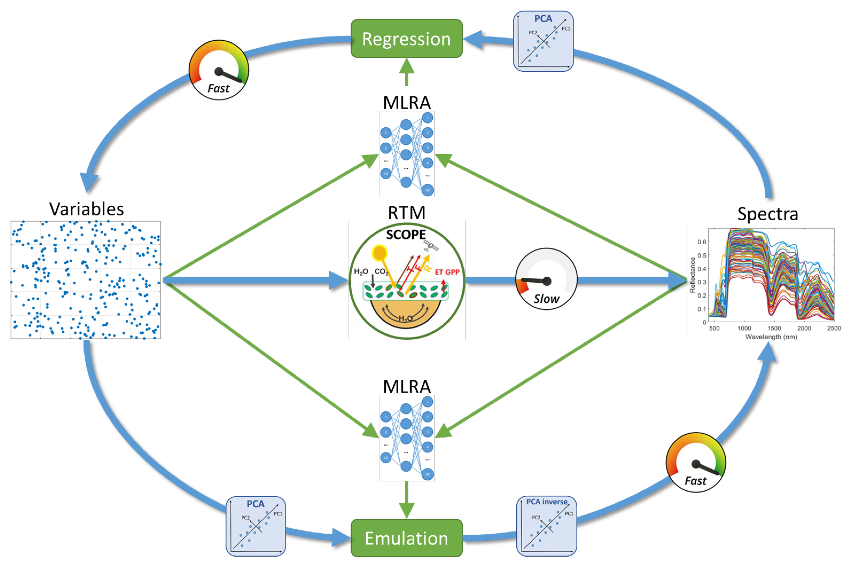
Figure 2.
Example of original simulations of (a) LESS TOC reflectance and (c) PROSAIL coupled with libRadtran TOA radiance, alongside 1000 randomly generated spectral outputs from their corresponding GPR emulators (b, d).
Figure 2.
Example of original simulations of (a) LESS TOC reflectance and (c) PROSAIL coupled with libRadtran TOA radiance, alongside 1000 randomly generated spectral outputs from their corresponding GPR emulators (b, d).
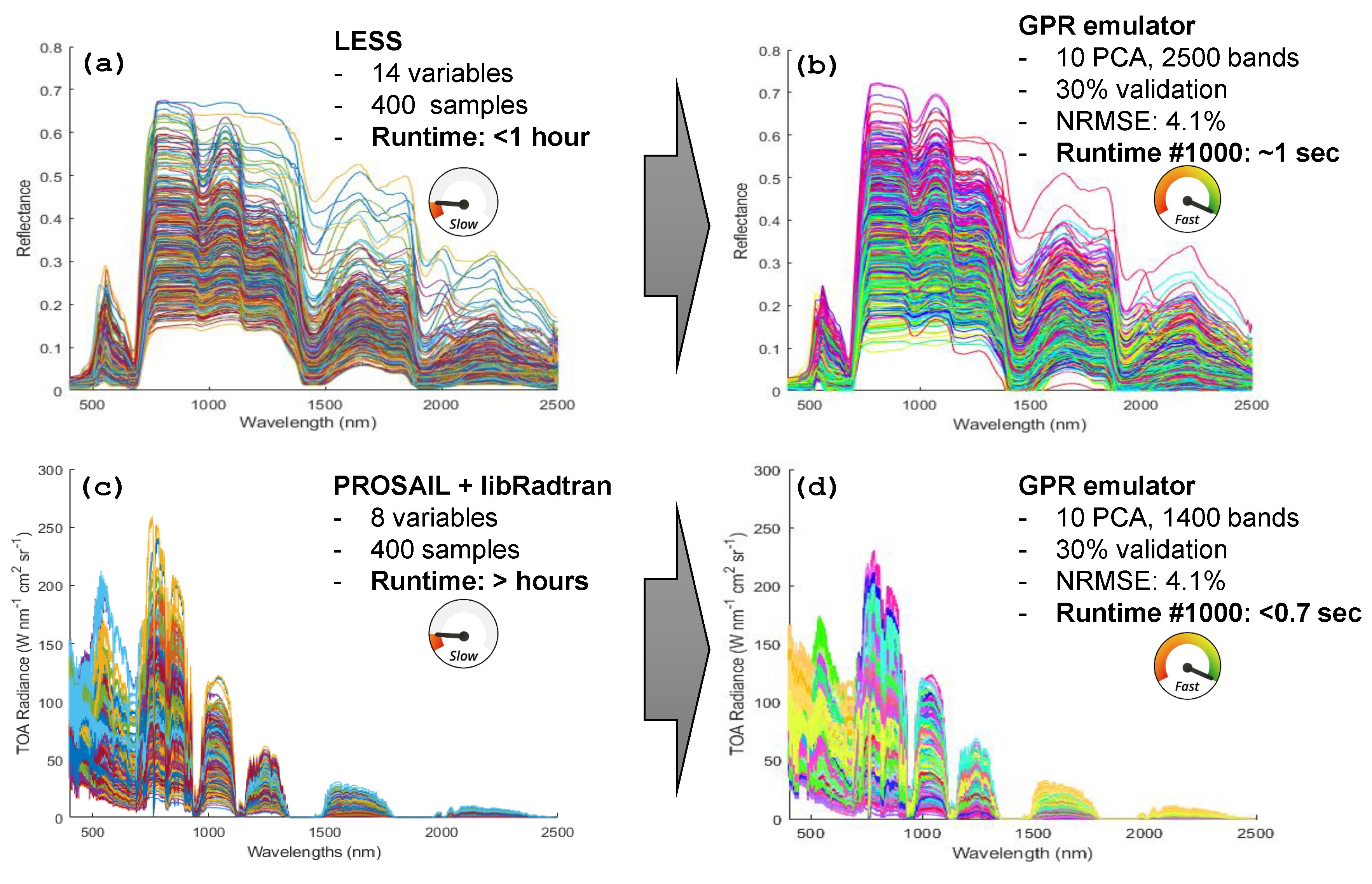
Figure 3.
Total sensitivity results of TOA radiance using a GPR emulator of a 12-variable PROSAIL-MODTRAN RTM. Figure is adapted from [136]: A GPR emulator was run in ARTMO’s GSA tool with 1000 samples per variable. The processing took less than 40 seconds. Figure is adapted from [136]; see [136] for details and interpretation.
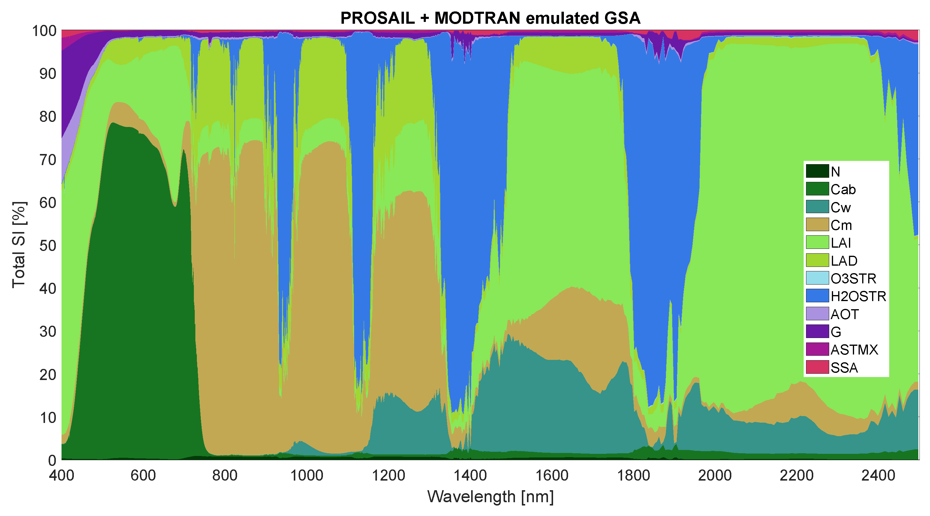
Figure 4.
Illustration of A-SGM scene generation by using emulators. First, a land cover map is arbitrarily created. Then, these classes are filled with the input variables as described in [61]. Following the emulators are run to generate the spectral datacubes. For illustration, output images of a few wavelengths are shown. General statistics (mean, SD, min-max) per class are derived. Figure is adapted from [61]; see [61] for details.

Figure 5.
Workflow showing the procedure of emulating hyper- from S2 multispectral data using an MLRA in combination with PCA dimensionality reduction and back-projection. Figure is adapted from [144]; see [144] for details.
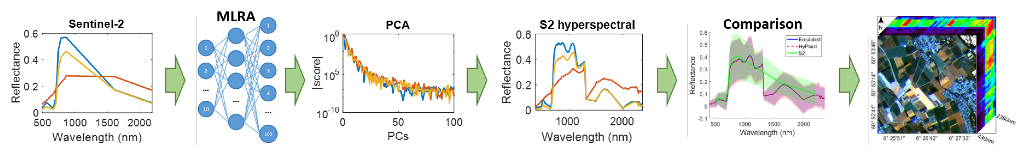
Figure 6.
Illustration of emulator-based numerical inversion over a forested terrain. A KRR emulator was trained based on DART simulations. The function ’lsqnonlin’ of Matlab’s optimization toolbox was used for the inversion. The traits FVC, LCC, and LAI were successfully retrieved, while the RMSE gives insight into retrieval quality. See [78] for details.
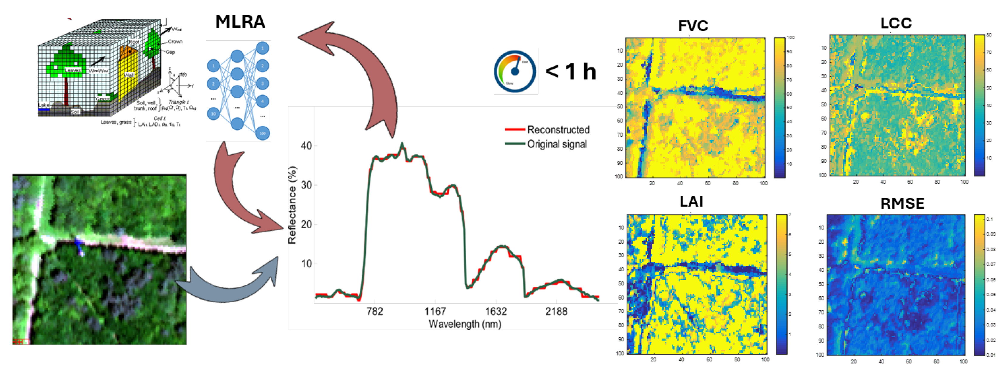
Table 2.
Comparison of MLRAs used for emulating RTMs, ordered from the most applied to the least.
| Method | Description | Pros | Cons | Example Emulation Use |
|---|---|---|---|---|
| Neural Networks (NNs) [59] | Flexible models that learn non-linear mappings through interconnected layers. | High scalability, captures complex patterns, optimized inference speed. | Requires large datasets, limited interpretability, approximate UQ, sensitive to hyperparameters. | Emulating complex RTMs (e.g., coupled vegetation-atmosphere models), scene-to-scene inversion [e.g., [26,42,60,61,62,63,64]]. |
| Deep Learning NNs (DLNNs) [65] | Advanced NN architectures including Convolutional NNs, Recurrent NNs, autoencoders, transformers, and physics-informed NNs. Designed for high-dimensional, spatiotemporal, or structured data emulation. | Extremely flexible, handles high-dimensional inputs, learns spatial/temporal structure, enables end-to-end inversion, supports uncertainty via dropout or ensembles. | Computationally demanding to train, it requires large annotated datasets, has reduced interpretability, and carries an overfitting risk. | Scene-level RTM emulation, spatiotemporal flux retrievals, hybrid physical–DL models (e.g., MODTRAN emulation with CNNs) [e.g., [66,67,68,69,70]]. |
| Gaussian Process Regression (GPR) [71] | Kernel-based probabilistic model providing both mean and variance predictions; ideal for small datasets and inherent UQ. | High accuracy, strong UQ, robust with small data, interpretable. | Scales as , memory-intensive, less suited for large datasets. | Emulating PROSAIL, SCOPE, MODTRAN in applications where accuracy and UQ is critical [e.g.,[26,27,42,60,61,63,72,73,74]]. |
| Random Forests (RF) [75] | Ensemble of decision trees that aggregate outputs for robust prediction. Well-suited for tabular and structured data. | Robust, fast training, interpretable via feature importance, handles noise. | No inherent UQ but empirical variance. Slower prediction at scale due to multiple decision trees, and tends to reduce the impact of outliers due to its averaging nature. | Used as alternative RTM emulators in some benchmarking studies [e.g., [61,76]]. |
| Kernel Ridge Regression (KRR) [77] | Ridge regression in a kernel-transformed space; similar to GPR but deterministic. | Competitive accuracy, captures non-linearity, less sensitive to hyperparameters. | Scales as , no native UQ, less popular than GPR. | Alternative to GPR for mid-sized RTMs where UQ is not essential [e.g., [60,61,69,78]]. |
| Support Vector Regression (SVR) [79] | Finds a hyperplane with -insensitive loss; effective in high-dimensional spaces with kernel trick. | Accurate, robust to outliers, generalizes well with good kernel choice. | Scales as , sensitive to kernel and hyperparameters, lacks native UQ. | Used for spectral emulation tasks with moderate-sized datasets [e.g., [61,76]]. |
| Polynomial Chaos Expansion (PCE) [80] | Expands model output in orthogonal polynomials based on input distributions, allowing for analytical UQ and sensitivity analysis. | Provides analytical UQ, Sobol indices, interpretable, and efficient for low dimensions. | Suffers from curse of dimensionality, basis tied to distribution, struggles with strong non-linearity. | Used in global sensitivity and UQ analysis of deterministic models. Not applied to RTMs. |
Table 3.
Comparison of common MLRAs for emulating RTMs: accuracy, uncertainty quantification (UQ), scalability, interpretability, and key references. UQ refers to whether the method natively provides principled predictive uncertainty or only empirical approximations.
Table 3.
Comparison of common MLRAs for emulating RTMs: accuracy, uncertainty quantification (UQ), scalability, interpretability, and key references. UQ refers to whether the method natively provides principled predictive uncertainty or only empirical approximations.
| Method | Accuracy | UQ | Scalability | Interpretability | RTM studies |
|---|---|---|---|---|---|
| NNs | High | Approx. (MC dropout, ensembles) | High | Low | [26,42,60,61,62,63,64] |
| DLNNs | Very High | Approx. (MC dropout, deep ensembles) | Very High | Very Low | [66,67,68,69,70] |
| GPR | High | Yes (Bayesian predictive distribution) | Limited | Medium | [26,27,42,60,61,63,72,73,74] |
| RF | Moderate–High | Empirical (ensemble variance) | High | Medium | [61,63,69] |
| KRR | High | No | High | Medium | [26,42,60,61,78] |
| SVR | Moderate–High | No | Medium | Medium | [61,76] |
| PCE | Moderate | Yes (analytical) | Moderate | High | No RTM studies |
Table 4.
Comparison of common space-filling sampling designs for emulator training in RTM applications.
Table 4.
Comparison of common space-filling sampling designs for emulator training in RTM applications.
| Property | Latin Hypercube Sampling (LHS) [105] | Sobol Sequence [106] | Halton Sequence [107] |
|---|---|---|---|
| Type | Stratified random sampling | Quasi-random (low-discrepancy) sequence | Quasi-random (low-discrepancy) sequence |
| Space-filling Quality | Good in all dimensions (by construction) | Excellent for moderate to high dimensions | Good in low dimensions; deteriorates with higher dimensions |
| Uniformity | Random, but forced stratification ensures uniform marginal distributions | Highly uniform; minimizes gaps and clusters | Uniform in low dimensions; suffers from correlation in higher dimensions |
| Determinism | Stochastic (can vary by seed) | Deterministic | Deterministic |
| Scalability | Easily scalable to high dimensions and sample sizes | Efficient in high-dimensional settings; extensible | Less scalable; performance degrades beyond 10–20 dimensions |
| Implementation Simplicity | Simple and widely implemented | Slightly more complex; supported in numerical libraries | Relatively simple but less widely used |
| Suitability for Emulator Training | Common choice due to flexibility and randomness | Preferred for high-dimensional RTMs due to uniformity and extensibility | Suitable for low-dimensional problems, less ideal for complex RTMs |
| Reproducibility | Depends on random seed | Fully reproducible | Fully reproducible |
| Use | Widely used for training | Used for running emulators in global sensitivity analysis (see also Section 4.2) | No RTM emulation studies |
Table 5.
Comparison of common dimensionality reduction techniques used in RTM emulation workflows.
| Property | PCA [112] | SVD [113] | Autoencoder [114] |
|---|---|---|---|
| Type | Linear projection | Linear matrix factorization | Nonlinear encoder-decoder |
| Learning | Unsupervised (closed-form) | Unsupervised (closed-form) | Unsupervised (trained with backpropagation) |
| Nonlinearity | No | No | Yes |
| Interpretability | High (ordered by variance) | Moderate (singular vectors) | Low (latent variables) |
| Scalability | Fast, memory-limited at scale | Efficient, scalable SVD libs. exist | Scales well; training cost higher |
| Compression | Effective for linear variance | Good for general matrices | Strong for nonlinear manifolds |
| Reconstruction | Inverse projection from PCs | Matrix product of truncated SVD | Decoder reconstructs from latent space |
| Accuracy | Good for linear data | Similar to PCA | Better for nonlinear data |
| Complexity | Simple, widely used | Simple, widely available | Requires architecture and tuning |
| RTM Use | Common for LUT/input reduction | Rare, yet applicable (similar to PCA) | Increasing use for LUT compression |
| References | [e.g., [60,121]] | – | [e.g., [66,69]] |
Table 6.
Overview of promising machine learning methods for RTM emulation. While not yet widely applied in RTM studies, these approaches offer potential due to scalability, uncertainty quantification, or structural flexibility. Refs: references.
Table 6.
Overview of promising machine learning methods for RTM emulation. While not yet widely applied in RTM studies, these approaches offer potential due to scalability, uncertainty quantification, or structural flexibility. Refs: references.
| ML Method | Type | Strengths for Emulation | Refs |
|---|---|---|---|
| Scalable GPR; e.g., Sparse GPR, nearest neighbor GPR (NNGPR), stochastic variational (SVGP) | Probabilistic kernel regression | Uncertainty quantification; scalable to large datasets via approximation | [122,123,124] |
| Deep GPR | Deep kernel-based regression | Captures hierarchical structure; better handles complex non-stationarity | [125] |
| Bayesian Additive Regression Trees (BART) | Bayesian ensemble trees | Probabilistic output; interpretable; handles nonlinear relationships well | [126] |
| XGBoost | Gradient-boosted decision trees (GBDTs) | Fast and accurate; robust to overfitting; interpretable | [127] |
| LightGBM | GBDTs with histogram splits | Very fast; handles large-scale input efficiently | [128] |
| CatBoost | GBDTs with ordered boosting | Effective with categorical inputs; competitive accuracy | [129] |
| CNNs | Deep learning (spatial) | Strong at extracting local spectral/spatial patterns; good for hyperspectral data | [130] |
| Transformers | Deep learning (attention) | Captures long-range interactions; suited to structured inputs (e.g., spectra) | [131] |
| PINNs | Physics-informed NNs | Incorporates RTM physics in training (e.g., spectral absorption features, conservation laws); enables physically consistent emulation | [132] |
| Bayesian Neural Networks (BNNs) | Probabilistic deep learning | Uncertainty-aware emulation; flexible for complex nonlinearities | [133] |
| Generative Adversarial Networks (GANs) | Generative deep learning | Capable of high-fidelity synthetic spectral generation; potential for inversion/data augmentation | [134] |
Disclaimer/Publisher’s Note: The statements, opinions and data contained in all publications are solely those of the individual author(s) and contributor(s) and not of MDPI and/or the editor(s). MDPI and/or the editor(s) disclaim responsibility for any injury to people or property resulting from any ideas, methods, instructions or products referred to in the content. |
© 2025 by the authors. Licensee MDPI, Basel, Switzerland. This article is an open access article distributed under the terms and conditions of the Creative Commons Attribution (CC BY) license (https://creativecommons.org/licenses/by/4.0/).
Copyright: This open access article is published under a Creative Commons CC BY 4.0 license, which permit the free download, distribution, and reuse, provided that the author and preprint are cited in any reuse.


