
Submitted:
09 September 2025
Posted:
10 September 2025
You are already at the latest version
Abstract
Adhesive wear leads to substantial material loss, presenting a significant challenge across various industries. To address this issue, it is crucial to conduct studies aimed at mitigating this degradation. This particular study focuses on achieving a high-quality product with minimal mass loss during adhesive wear by utilizing gas nitriding treatment to optimize the wear parameters of 42CrMo4 steel. The study employed the Taguchi methodology and response surface methodology (RSM) to design the experiments. Key wear parameters, including wear speed (V), normal load (FN), and the microhardness of nitrided parts (HV), were thoroughly investigated. Additionally, an artificial neural network (ANN) prediction model was developed to forecast the wear performance of 4140 Steel. The ANN model demonstrated an accuracy of approximately 99% when compared to the experimental data. To further enhance the precision of wear estimation, prediction optimization was conducted using Bayesian and genetic algorithms. The results showed that the predicted R² values aligned reasonably well with the adjusted R² values, with a difference of less than 0.2. The analysis revealed that the normal load is the most critical factor influencing wear, followed by hardness, while wear speed has the least significant impact.
Keywords:
gaseous nitriding
; adhesive wear
; 4140 steel
; optimization
; prediction
; artificial neural network
1. Introduction
Wear remains a significant challenge in various industrial sectors, including automotive, biomedical, aeronautics, and aerospace, as it jeopardizes the performance and lifespan of mechanical steels [1-3]. Adhesive wear, which occurs when hard and sharp particles come into contact with a softer surface, causing its detachment, is one of the primary modes of wear. This phenomenon results in material, shape, and functional losses of parts, which can have detrimental consequences on the safety, reliability, and efficiency of the mechanical systems in which they are integrated. Therefore, it is essential to conduct studies aimed at minimizing this degradation. To reduce adhesive wear, the surface of parts can be modified through thermochemical treatments, such as enriching the surface layer with elements like nitrogen, carbon, or boron.
The thermochemical treatment used in this context is gas nitriding. This process, which enriches the steel surface with nitrogen at relatively low temperatures, reduces the risk of part deformation. It allows the formation of iron nitrides or other alloy elements, creating two layers on the steel surface: a combination layer (white layer) and a thicker diffusion layer [6, 7]. These layers enhance hardness, providing betterresistance to wear, corrosion, and fatigue [6-8]. This treatment offers advantages in terms of cost, simplicity, and efficiency. Particular attention has been given to 4140 steel, a construction steel alloyed with chrome and molybdenum, known for its good hardenability and resistance to fatigue and wear [9-11]. This makes it ideal for applications such as gears and crankshafts. Wear tests were conducted to measure the mass loss during adhesive wear of samples over time, evaluating the effectiveness of gas nitriding treatment in reducing wear.
Optimization has become a crucial component in various industries, highlighting the usefulness of dynamic modeling tools over static ones. Predictive modeling, which uses statistical algorithms to predict outcomes, is increasingly integrated into these optimizationtools. This integration enables industries to anticipate future trends, make proactive decisions, and improve operational efficiency [12-16].Several statistical techniques have been introduced for parameter optimization. For instance, response surface methodology (RSM) was applied to determine the optimal temperature and hydrogen deposition rate for producing diamond-like carbon (DLC) coatings with low friction coefficients and high wear resistance. Taguchi statistical techniques were used to study the wear and friction properties of MoS2 coatings on laser-textured surfaces.
The effectiveness of RSMoptimization was compared to recognized machine learning techniques, including artificial neural networks (ANN) and genetic algorithms (GA), with ANN providing more accurate predictions. This study examines the impact of various parameters on the wear of AISI 4140 steel parts treated with gas nitriding, including hardness, normal load, and wear speed. Taguchi statistical analysis tools were used to identify the dominant factors affecting mass loss during adhesive wear. An ANN neural network was developed using Matlab to predict mass loss, with different network configurations tested for accuracy. The genetic algorithm and Bayesian algorithm were employed to optimize the prediction of wear, enhancing the accuracy of wear estimation.
This research offers an innovative approach to minimizing wear, which could have significant implications for the industry by extending the lifespan of components and improving system reliability. It also paves the way for new research on the optimization of surface treatments for other types of materials.
2. Materials and Methods
2.1. Material and treatments
4140 steel, a low-alloy steel that complies with the European standard, was chosen as the study material for this research. The detailed chemical composition of this material is presented in Table 1.
The main parameters of the gaseous nitriding treatments applied to a series of 42CrMo4 steel wear specimens are summarized in Table 2. The filiations of Vickers micro-hardness using a SHIMADZU-HMV-2000 under a 50gf (HV0.05), on cross-section, allow to control the efficiency of each treatment through the determination of the surface hardness (HV max) and the hardened depth. The results corresponding to each nitriding treatment are gathered in Table 2.
Wear tests were performed by the double weighing method, on a wear bench, the specimens rubbing on a wheel animated by a constant speed rotation under the action of a load. The sample is fixed on the sample holder, the latter is free in translation, and the load is transmitted to it under the effect of a calibrated spring. The test bench, crafted from X160CrMoV12 material, is distinguished by its hardness of 58 HRC and a roughness Ra of 0.4 µm. As for the test specimens used for the tests, they have an identical diameter and length of 15 mm. It should be noted that the wear test is carried out under dry friction conditions at room temperature, thus ensuring an accurate evaluation of the material’s resistance.
2.2. Methodology:
The influence of wear parameters on mass loss during adhesive wear is examined in the study. Three main factors are taken into account: the microhardness of the nitrided parts (HV), the Normal load (F) and the wear speed (V). Each of these factors is studied at different levels. Table 3 presents these factors, as well as their type and level.
To optimize the responses more efficiently, the Taguchi plan and the RSM method, both methods of experiment planning, were used. This method allows to find the best result with the minimum possible tests [11]. A series of 24 tests was carried out, each identified by a distinct number from 1 to 24. The experiment plan that best matched the input parameters was selected, built and completed with the corresponding response mass loss (∆M/M (%)), which represents the mass loss following the wear test.
2.3. Prediction by neural network
Artificial neural networks (ANNs) function in a manner similar to the human brain, utilizing weights and biases to perform highly nonlinear functions [12]. Currently, ANNs are employed to solve a wide range of complex engineering problems. They are capable of learning by example, making them highly useful for simulating correlations that are challenging to describe with physical models or other mathematical approaches. Although perfect prediction is rarely achievable, neural networks can provide reasonably good predictions in many cases [13]. ANN methods are commonly utilized in various fields such as modeling, simulation, learning, definition, and prediction [14]. For instance, ANNs have been used to predict the wear behavior of materials, with a significant body of literature already published in this area of research [20]. The neural network, noted for itscompactness and simplicity, is recognized as an effective tool for predicting mass loss. To achieve the most accurate predictions possible, variations in the parameters of the neural network were implemented, including changes to the activation function, algorithms, and the number of hidden layers and neurons.
Based on the analysis of the experimental results, it is clear that the normal load (F), the sliding speed (V), and the maximum surface microhardness (HV) are the most critical factors for studying the wear resistance of nitrided layers. These factors thus constitute the inputs of the neural network. The experimental data collected for this study are divided into three sets: a training dataset (70%), a test dataset (15%), and a validation dataset (15%) [20]. The experimental design includes 135 tests: 95 are used for training the network and 20 are arbitrarily chosen to validate and test the network. Regarding the architecture of the artificial neural network (ANN), different structures have been proposed for process modeling, such as the multilayer perceptron (MLP) and the radial basis function (RBF). In this study, an ANN using the feed for ward back-propagation algorithm was adopted for modeling and testing using MATLAB software. We will subsequently examine architectures with different numbers of hidden layers and different numbers of neurons in each hidden layer for the three chosen activation functions.
Hyperbolic: an S-shaped mathematical function, takes real values as input and returns values between -1 and 1.
Sigmoid: also S-shaped, takes real values as input and returns values between 0 and 1.
Linear: returns the same value that it receives as input and is often used in the last layer of a neural network for regression tasks.
After choosing the activation function, we determine the variables measuring performance for each combination for the different learning algorithms [11]: TRAINLM: learning by the Levenberg-Marquardt algorithm (quasi-Newton method),TRAINSCG: learning by scaled conjugate gradient (SCG) and TRAINBR: version of trainlm but with automatic weight moderation. The architecture and details of the neural network are illustrated in Table 4. The internal architecture of the three layers is illustrated in Figure 1.
The performance of the algorithms will be measured for each combination of hidden layers and the number of neurons for each activation function. The results obtained from these combinations will be collected and compared, and the best possible result from each algorithm for the three hidden layers will be extracted. These data will be summarized in Table 4.
In Table 4, the correlation coefficient R and the mean squared error (MSE) will be indicated. The MSE, used as a cost function, will help determine which combination best fits the problem of predicting mass loss. The expression for MSE is as follows:
Thus, we calculated the square root RMSE (Root Mean Squared Error) to compare them and choose the best possible result. Its expression is indicated below :
3. Results
3.1. Surfaces responses
The examination of the response table for raw signal ratios (Table 5) allows us to deduce that normal load is the most significant factor affecting material loss, followed by hardness and then wear speed. This suggests that it would be wise to first focus on normal load, then on hardness, and finally on speed to optimize experimental conditions and minimize mass loss. Indeed, the graphical analysis of the main effects for raw signal ratios (Figure 2.a) shows that the maximum mass loss is reached for a maximum normal load level of 175N. Similarly, the minimum mass loss is reached for a minimum hardness of 895 HV.
These two factors therefore have a significant impact on mass loss. Similarly, it was observed that the hardness of the steel, measured at 1090HV and obtained by gas nitriding over a period of 24 hours, allowed to minimize the mass of the steel while obtaining a satisfactory result in terms of resistance and durability. On the other hand, when a part was nitrided to a hardness of 930HV for a longer period of 36 hours, the result was less satisfactory.
This can be attributed to a phenomenon known as nitrogen saturation. During nitriding, nitrogen is incorporated into the surface layer of the steel. However, there is a limit to the amount of nitrogen that the steel can absorb. These results indicate that the increase in hardness obtained by gas nitriding is very significant and can positively influence the results by significantly reducing mass loss during adhesive wear. To do this, it is important to choose the nitriding conditions well, taking into account time constraints.
In the Pareto diagram (Figure 2.b), a significance limit of 2.131 is established. The effects of factors considered statistically significant are represented by bars that exceed this limit. The most important factors, ranked in descending order of importance, are normal load, hardness, and speed. The square of hardness is also considered statistically significant. The effects of factors that are not considered statistically significant are represented by bars that do not exceed the significance limit. These factors, having a lesser effect on the studied response, can be ignored from the analysis, it is important to note that the interactions between these factors are not statistically significant. This means that the combined effect of these factors on the studied response is not significant enough to be considered significant.
3.2. Regression equation
An alternative approach was explored using the genetic algorithm to optimize the variables of the adjustment equation proposed by Minitab. This algorithm, which draws its inspiration from the biological principles of evolution, notably natural selection, has proven to be a very effective optimization technique. The genetic algorithm works by systematically modifying the variables of the adjustment equation, following a specific program. This process is similar to how genes are modified over generations in the process of natural evolution. The goal of this systematic modification is to achieve the greatest possible accuracy between the experimental and optimal models, taking into account several factors simultaneously, such as normal load, hardness, and speed, the algorithm was able to further optimize the response. Here is the obtained regression equation:
∆M/M(%) = 14.5 - 0.0276 × HV - 0.00005 × FN - 0.088 × V + 0.000013 × HV2 + 0.000008 × FN2- 0.0000009 × HV × FN + 0.000092 × HV × V + 0.000129 × FN × V.
3.3. RSM method
3.3.1. Regression Models
Table 6 display the multiple regression coefficients (R²) derived from the least squares technique to predict the model based on the second-order polynomial. The P values (<0.05) indicate that the effects resulting from hardness and normal load are significant. The R² values show that the regressed models are acceptable and adequately correspond to the experimental data. Additionally, values greater than 0.1 indicate that the model terms are not significant. The experimental and predicted results are found to be approximately the same.
The F value of the model, 6.84, implies that the model is significant. There is only a 0.24% chance that such a large F value could occur due to noise (Table 6). The predicted R² of 0.3119 is in reasonable agreement with the adjusted R² of 0.4323, with the difference being less than 0.2. The Adeq Precision, which measures the signal to noise ratio, is 8.999, indicating an adequate signal. A ratio greater than 4 is desirable, and this model can be used to navigate the design space.
The hardness, normal load, and wear speed are dependent on the effects obtained from the linear quadratic and the interaction of the studied variables. Consequently, after taking into account the determined coefficients, the one provided in equation (6) is expressed by:
∆M/M(%) = 0.1379 — 0.0462 × HV + 0.0787 × F + 0.0250 × V
3.3.2. Effect of independent variables on mass loss
Figure 3 displays the normal probability plots of mass loss, generated from the CCD matrix. These plots reveal a pronounced linear trend with minimal deviations from the regression line, indicating a strong linear correlation. Even extreme values adhere to this trend, reinforcing the notion of a robust linear relationship. Additionally, no significant outliers were observed compared to the normal distribution, confirming the validity of the CCD matrix for parameter interaction (P > 0.05).
Figure 4 presents a three-dimensional (3D) model and plot surfaces, As shown in Figure 5a, increasing the hardness of the parts at a fixed wear speed of 6.24 m/s and a fixed normal load of 137.5 N reduces mass loss to -0.1, due to the textural and morphological modification of the white layer and the nitriding diffusion layer, as confirmed by several authors [22]. Increasing the normal load for a fixed hardness of 798 HV up to 122.5 results in a mass loss of 0.2%, and a further increase to 182.5 leads to dangerous wear above 0.3%. Similarly, increasing the wear speed to 4.78826 m/s for a constant hardness of 572.746 HV also results in dangerous wear above 0.3%.
However, For a hardness greater than 964 HV, the wear speed does not have a notable influence. Figure 5c illustrates both the normal load and wear speed at a fixed hardness of 994 HV. A wear force varying from 170 to 212.5 and a wear speed varying from 5 to 10 m/s result in catastrophic wear and a mass loss reaching 0.4%. The interaction between these two variables led to a weak layer.
The response optimizer, illustrated in Figure 5, is an effective tool for determining the optimal values of several parameters, including hardness (H), normal load (F), and speed (V). In order to validate the predictions of this tool, confirmation experiments were conducted using the optimal parameters predicted by the response surface method (RSM). The optimal values obtained were 1075.85 HV for hardness, 101.532 N for normal load, and 4.24848 for speed, producing a response of 0.00036. These results confirm the effectiveness of the response optimizer in predicting optimal conditions.
3.4. Artificial Neural Network models
3.4.1. Prediction
Table 7 provides a detailed overview of the most reliable predictions, which are those that display correlation coefficients approaching a maximum of 1 for each algorithm and each number of hidden layers for the three activation functions. These predictions are based on the training, validation, and test phases. To prevent over fitting (where the prediction model adapts too well to the training data, losing its ability to generalize correctly to new data), the mean square error (MSE) and its square root (RMSE) are calculated subsequently. This approach ensures that the model's performance is evaluated comprehensively to avoid over fitting.
After evaluating these results by comparing the parameters measuring the robustness, reliability, and performance of the neural network, it was found that the sigmoid function with the Bayesian regularization algorithm that uses the ‘trainbr’ function for learning with the following network structure: 12 neurons at the input, 2 hidden layers (12 trainbr 2), allows obtaining a correlation coefficient close to 1, as well as the minimum of the mean square error value which is 0.000321.
Figure 6 presents the plots of the experimental values as a function of their corresponding predicted values. By analyzing this figure, it is observed that the intersection points between the experimental values and the estimated values are very close to the median line for the training and validation sets, which proves the effectiveness of the ANN model. After verifying the best result obtained by the neural network, the value obtained by the prediction was compared to that obtained experimentally.
This comparison made it possible to verify the accuracy of the prediction model compared to the experimental data and to analyze the differences between the two. The quality of the prediction model was thus able to be evaluated and adjustments were made if necessary to improve its accuracy. To perform this comparison, a curve was plotted representing the values obtained by the prediction and the values obtained experimentally. This curve made it possible to visualize the differences between the two data sets and to evaluate the quality of the prediction model.
The prediction curve presented in Figure 7 is well adjusted to the experimental curve. This observation allows concluding that the prediction model is very accurate and reliable. Similarly, the curves representing the evolution of mass loss as a function of the test conditions of the experimental and predicted values are almost perfectly superimposed. This observation indicates that the prediction model is both accurate and reliable.
In what follows, Figure 8 presents the appearance of the variation of mass loss obtained by the experimental study and predicted by the retained neural system as a function of the test parameters that have a notable influence, namely: normal load F, wear speed Vg, and test duration for the different states of gas nitriding treatment studied (NG12, NG24, NG36).
3.4.2. Optimization of the prediction by neural network
We will work with a plan of 27 trials, numbered from 1 to 27. After choosing the experimental plan corresponding to the input parameters and constructing this plan, we will fill it with the response correlation coefficient R, These factors, as well as their type and level, are presented in Table 8.
In this study, initial predictions were generated using MATLAB software. The main objective was the optimization of these predictions by identifying the best combination of parameters - the activation function, the algorithm, the number of hidden layers, and the number of neurons - that maximizes the correlation coefficient R. Two distinct optimization algorithms were implemented to achieve this objective: the Bayesian algorithm and the genetic algorithm. the Bayesian algorithm and the genetic algorithm. Bayesian networks (BN) stand out as robust probabilistic graphical models for modeling and reasoning [22].
On the other hand, the genetic algorithm, an optimization method inspired by Darwin’s theory of evolution, was used to maximize the correlation coefficient R. This algorithm uses techniques such as selection, mutation, and crossover to generate a population of possible solutions. After 400 iterations, a correlation coefficient of 0.9962 was obtained (Figure 9.) The optimal parameters were a hyperbolic activation function, the Trainbr algorithm, eleven hidden layers, and two neurons.
Figure 10 is a graph that shows the evolution of the mean square error over generations. There are error peaks at certain points, indicating a sudden increase in error at these specific generations.
The same optimal solution was found by these two algorithms, despite their different approaches. This highlights not only the efficiency of each individual algorithm, but also the power of their combined use. When comparing these two algorithms, it was observed that the Bayesian algorithm is more focused on exploiting existing information to make precise adjustments, while the genetic algorithm is more focused on exploring possible new solutions. The use of these two algorithms in parallel allows for both exploitation and exploration, leading to more robust and precise solutions.
3.4.3. Comparison of predicted and experimental values
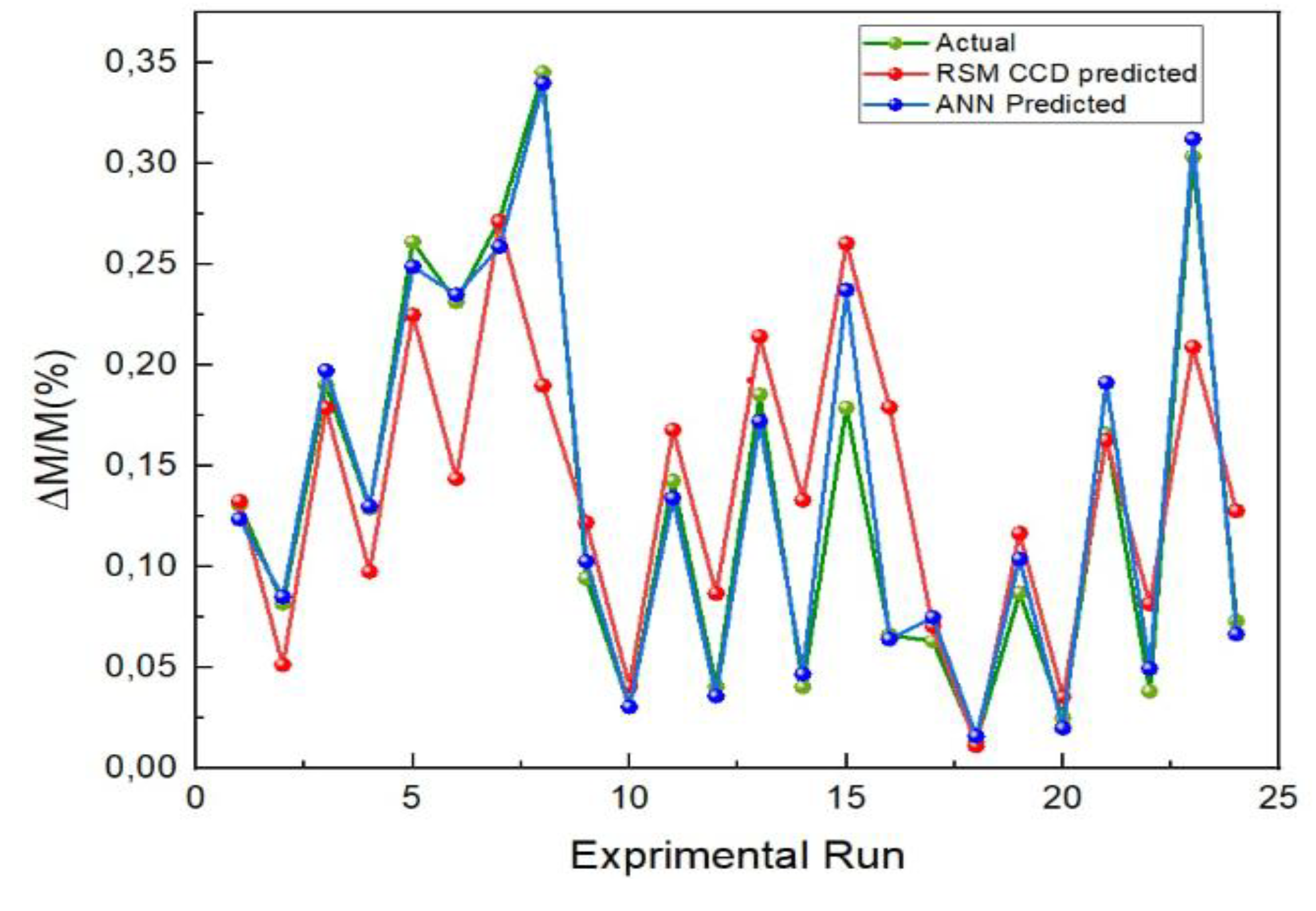
The ANN prediction curve shows a good fit with the experimental curve, which allows us to conclude that the accuracy of the prediction model is remarkably similar to the experimental data and very satisfactory. It is observed that the ANN method predicted the result more accurately than the RMS CCD method, which is also remarkable as can be seen from the error in Figure 11. On the other hand, a very large margin of error is observed for the linear regression method.
Figure 11.
Comparison of predicted and actual values.
4. Conclusions
The objective of this study was to have the effect of normal load, hardness, and speed on mass loss during adhesive wear of steel analyzed. An experimental method based on a design of experiments, as well as a numerical method based on an artificial neural network, was utilized. Data analysis revealed that normal load, hardness, and speed are significant factors. The most influential factor was identified as the normal load, followed by hardness and speed. The maximum mass loss was found to be obtained at a maximum force of 175 N, while the minimum mass loss was obtained at a minimum hardness of 895 HV.
The importance of hardness was highlighted by the observation that the hardness of the steel, achieved through gas nitriding for 24 hours, allowed for the minimization of mass loss while satisfactory results in terms of resistance and durability were obtained. However, nitriding at a hardness of 930 HV for a longer period of 36 hours was found to be less satisfactory, resulting in a loss of time and money due to nitrogen saturation. It was found that the increase in hardness obtained by gas nitriding can significantly reduce mass loss during adhesive wear. Therefore, it is important to choose the nitriding conditions well, taking into account time constraints.
The optimization of the variables of the regression equation, characterized by its quadratic structure, was carried out using a genetic algorithm. The optimization of the prediction showed that the optimal result by the neural network was obtained with a hyperbolic activation function, the trainbr algorithm, three hidden layers, and 11 neurons at epoch 27. Satisfactory and very accurate results were provided by the ANN method, which aligned well with the experimental results. In contrast, the prediction by the genetic algorithm was found to be the least accurate, suggesting thatalthough the genetic algorithm may be useful for certain types of problems, it is not the most appropriate for this particular case of studying the wear of steel.
Declaration of Competing Interest
The authors declare that they have no known competing financial interests or personal relationships that could have appeared to influence the work reported in this paper.
Funding
This work was supported and funded by the Deanship of Scientific Research at Imam Mohammad Ibn Saud Islamic University (IMSIU)(grant number IMSIU-DDRSP2503).
Acknowledgments
This work was supported and funded by the Deanship of Scientific Research at Imam Mohammad Ibn Saud Islamic University (IMSIU)(grant number IMSIU-DDRSP2503).
References
- B.Wang, X.Zhao, W.Li, M.Qin, and J.Gu "Effect of nitrided-layer microstructure control on wear behavior of AISI H13 hot work die steel" Applied Surface Science, 2017, pp.2-6.
- L.I. Kuksenova and M.S. Michugina "Effect of heating conditions in nitriding on the structure and wear resistance of surface layers of steel 38Kh2MyuA". Metal Science and Heat treatment, 2008, Vol.50, pp.68-72.
- O.A. Zambrano, Y. Aguilar, J. Valdés,, S.A. Rodríguez, and J.J. Coronado "Effect of Normal Load on Adhesive Wear Resistance and Wear Micro-mechanisms in FeMnAlC" Alloy and Other Austenitic Steels. Wear, 2016, Vol. 348-349, pp.61-68.
- M. A. Terres, H. Sidhom, A. Ben Cheikh Larbi and H. P. Lieurade "Tenue en fatigue flexion d’un acier nitruré". 2003, Vol.28(1), pp.25–41.
- G. Straffelini, G. Avi and M. Pellizzari "Effect of three nitriding treatments on tribological performance of 42CrAlMo7 steel in boundary lubrication". Wear, 2002, Vol.252, pp.870-879.
- A.E. Zeghni and M.S.J Hashmi. "The Effect of Coating and Nitriding on the Wear Behaviour of Tool Steels". Journal of Materiels Processing Technology, 2005, Vol.155-156, pp.1918-1922.
- M.A. Terres, R. Bechouel and S. Ben Mohamed «Low Cycle Fatigue Behavior of Nitrided Layer of 42CrMo4 Steel" International Journal of Materials Science, 2014, Vol.6(1) (2017), pp.18-27.
- M.A. Terres, H. Sidhom, A.B.C. Larbi, S. Ouali and H.P. Lieurade "Influence de la résistance à la fissuration de la couche de combinaison sur la tenue en fatigue des composants nitrurés" Matériaux & Techniques; 2001, Vol.89 (9-10), pp.23-36.
- X. Lu, Z. Jia, H. Wangand S.Y. Liang "The Effect of Cutting Parameters on Microhardness and the Prediction of Vickers Hardness Based on a Response Surface Methodology for Micro-milling Inconel 718". Measurement, 2019, pp.57-62.
- S. Vikram and S.K.Pradhan "Optimisation des paramètres WEDM à l’aide de la technique Taguchi et de la méthodologie de surface de réponse dans l’usinage de l'acier AISI D2". Procedia Engineering, 2014, Vol. 97, pp.1597-1608.
- V. Singh and S. K. Pradhan, "Optimization of WEDM parameters using Taguchi technique and Response Surface Methodology in machining of AISI D2 Steel". Procedia Engineering, 2017, Vol.97, pp.1597-1608.
- N. Mondal,, G. Nishant, M. C. Mandal,, S. Pati and S. Banik. "ANN and RSM based predictive model development and EDM process parameters optimization on AISI 304 stainless steel". Materials Today: Proceedings. Jalpaiguri Government Engineering College, Birla Institute of Technology, 2023.
- Shebani and, S. Iwnicki, (2018). "Prediction of wheel and rail wear under different contact conditions using artificial neural networks". Wear, 2018, Vol.406-407, pp.173-184. [CrossRef]
- Palavar, D. Özyürek and A. Kalyon, (2018). "Artificial neural network prediction of aging effects on the wear behavior of IN706 superalloy". Journal of Materials Research and Technology,2018, Vol. 7(4), pp.456-467. [CrossRef]
- M. Ebrahimi, F. Mahboubi and M.R. Naimi-jamal, "RSM base study of the effect of deposition temperature and Hydrogen flow on the wear behavior of DLC films", Elsevier 2015. [CrossRef]
- Dawit Zenebe Segu, Jong-Hyoung Kim, Si Geun Choi, Yong-Sub Jung and Seock Sam Kim, "Application of Taguchi Techniques to Study Friction and Wear Properties of MoS2 Coatings Deposited on Laser Textured Surface", Surf. Coat. Technol. 2013. [CrossRef]
- K. S.Ravikumar,, Y. D. Chethan, C. Likith and S. P. Chethan, (2023). Prediction of wear characteristics for Al-MnO2 nanocomposites using artificial neural network (ANN)." Journal of Materials Research and Technology, 2023, Vol.12(3), pp.456-467. [CrossRef]
- Laouissi, M. Nouioua, M.A. Yallese, H. Abderazek, H. Maouche and M.L. Bouhalais, "Machinability study and ANN-MOALO-based multi-response optimization during Eco-Friendly machining of EN-GJL-250 cast iron", Int J. Advan Man. Techn, 2021, Vol.117 (3- 4), pp.1179–1192.
- Laouissi, M.A. Yallese, A. Belbah, S. Belhadi, A. Haddad, "Investigation, modeling, and optimization of cutting parameters in turning of gray cast iron using coated and uncoated silicon nitride ceramic tools. Based on ANN, RSM, and GA optimization", Int J. Advan Man. Tech. 2019, Vol.101 (1-4), pp.523–548.
- S.O. Sada, "Improving the predictive accuracy of artificial neural network (ANN) approach in a mild steel turning operation", Int J. Advan Man. Tech. 2021, Vol.112 pp.2389–2398.
- Souid, W. Jomaa and M.A. Terres. Artificial neural network-based modeling and prediction of white layer formation during hard turning of steels. Matériaux & Techniques, 2024, Vol 112, 304.
- Ravikumar K., S. Chethan, Y. D., Likith, C., &Chethan, S. P. (2023). Prediction of wear characteristics for Al-MnO2 nanocomposites using artificial neural network (ANN). Journal of Materials Research and Technology, 2023, Vol.12(3), pp.456-467. [CrossRef]
Figure 1.
Internal architecture of the neural network : (a) one layer, (b) two layers and (c) three layers.
Figure 1.
Internal architecture of the neural network : (a) one layer, (b) two layers and (c) three layers.

Figure 2.
Main effects : (a) plot for signal-to-noise ratios and (b) Pareto diagram.
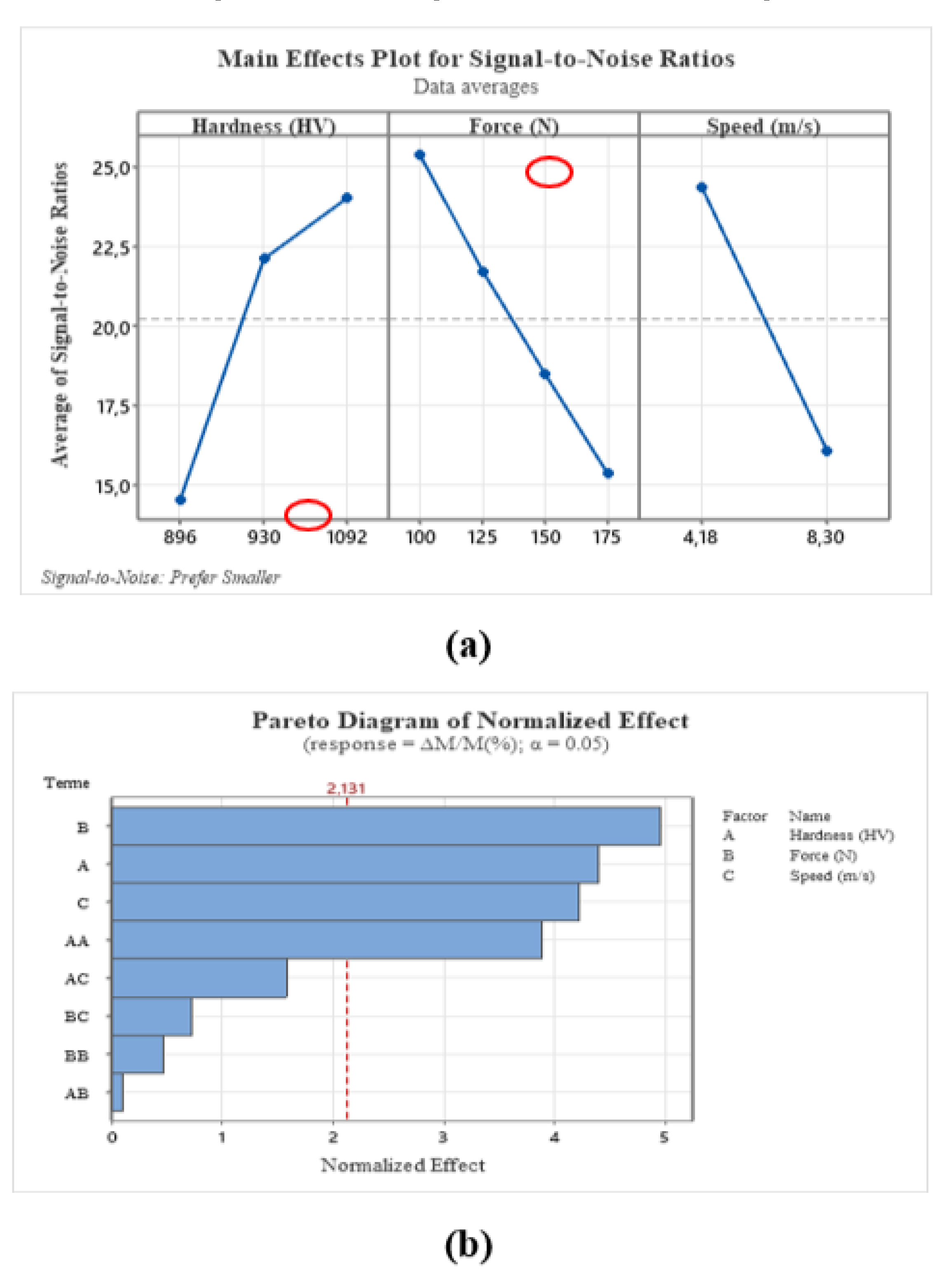
Figure 3.
Normal probability versus residual.
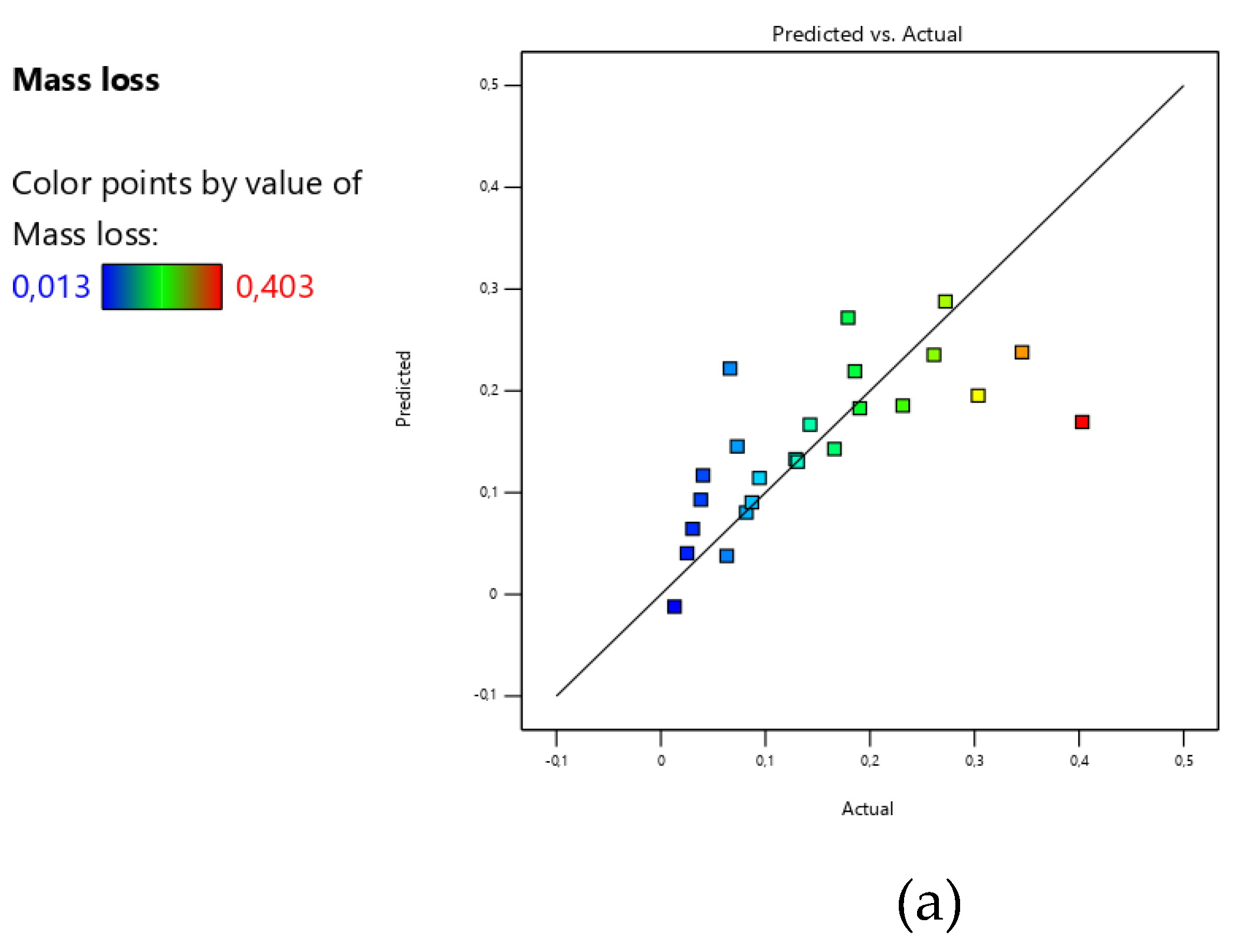
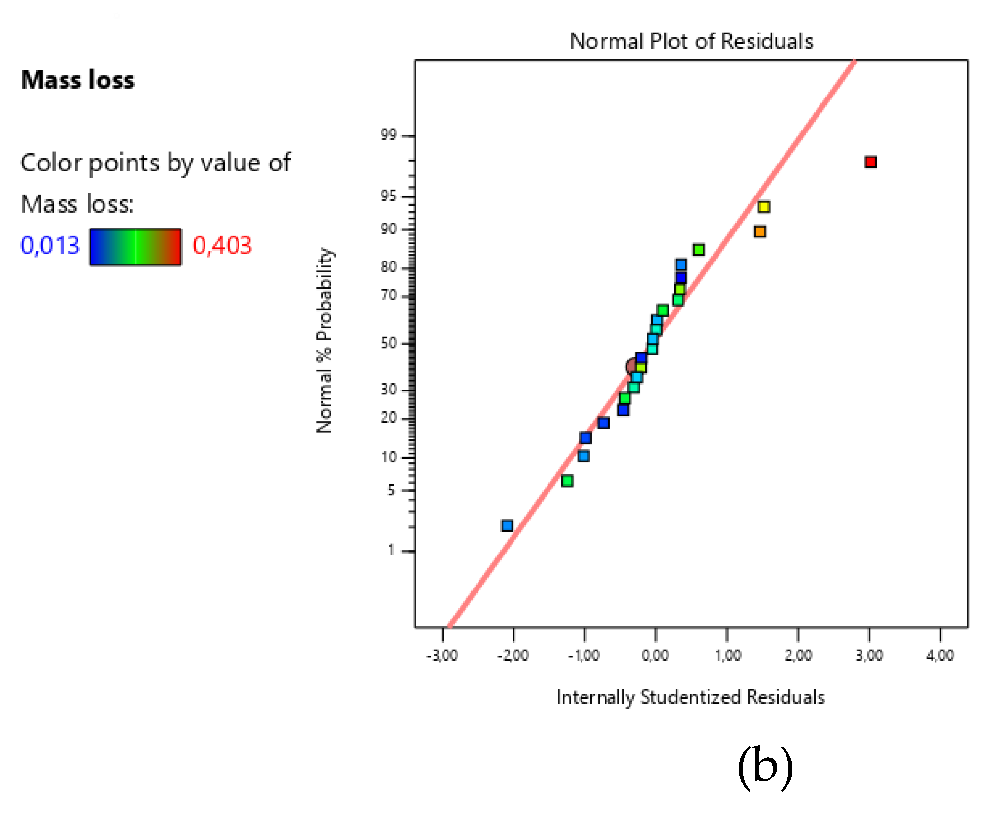
Figure 4.
Surface plot and its corresponding contour plot showing the interactions between the variables affecting Mass loss: (a) interaction H-F, (b) interaction H-V and (c) interaction F-V.
Figure 4.
Surface plot and its corresponding contour plot showing the interactions between the variables affecting Mass loss: (a) interaction H-F, (b) interaction H-V and (c) interaction F-V.
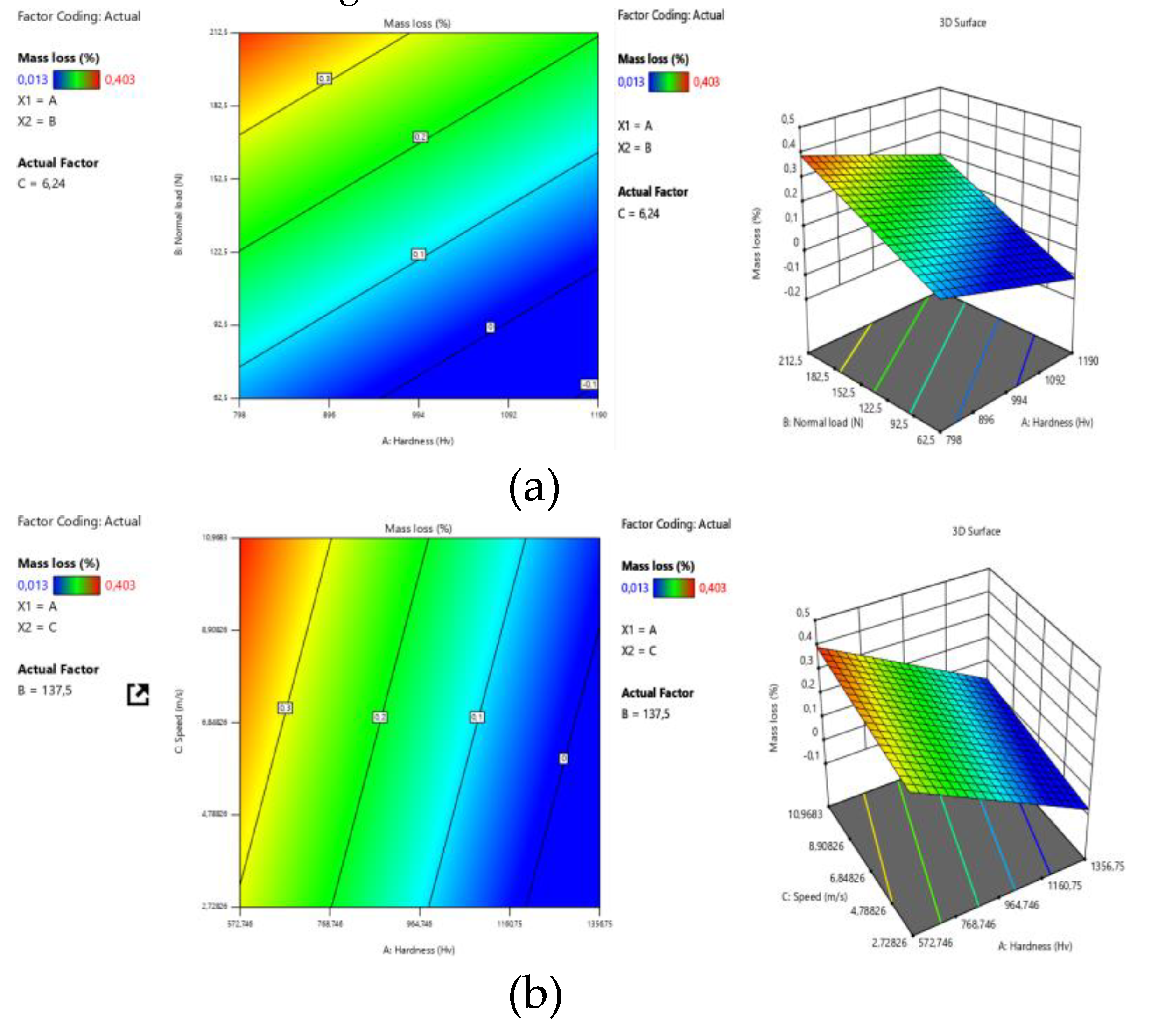
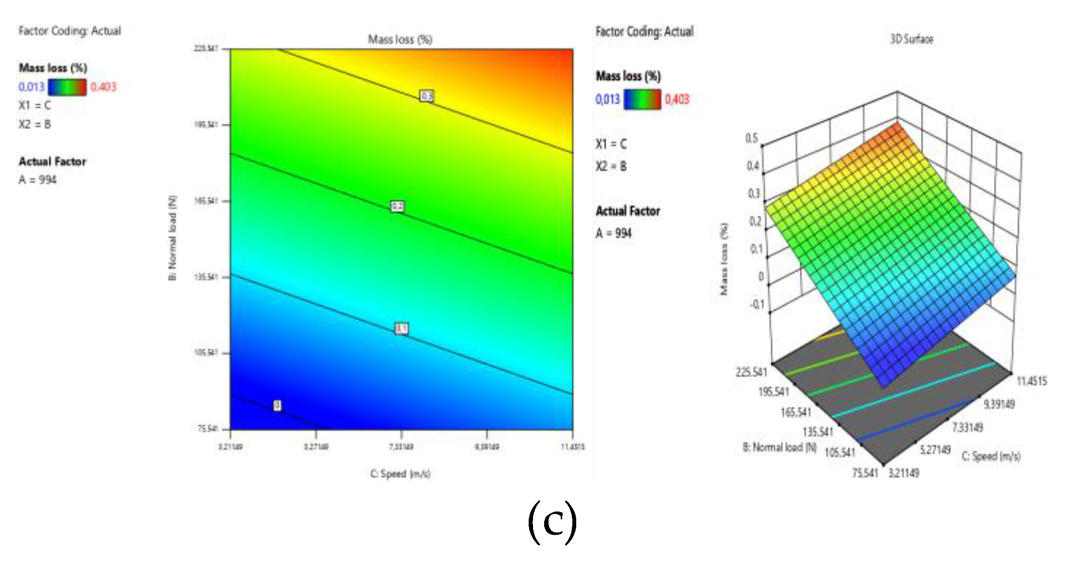
Figure 5.
Specific value for all responses under the optimized conditions.
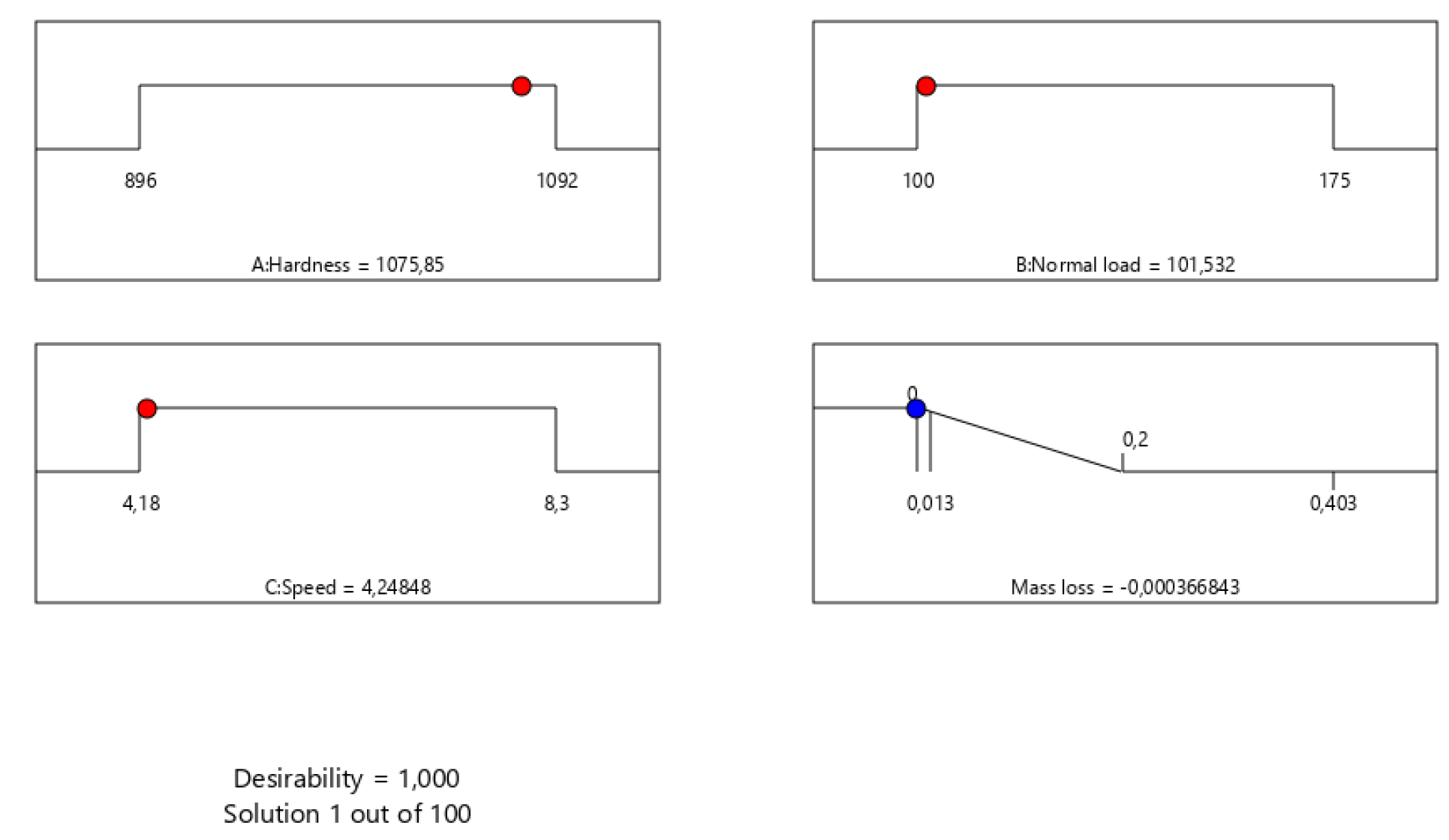
Figure 6.
Experimental values as a function of their predicted values.
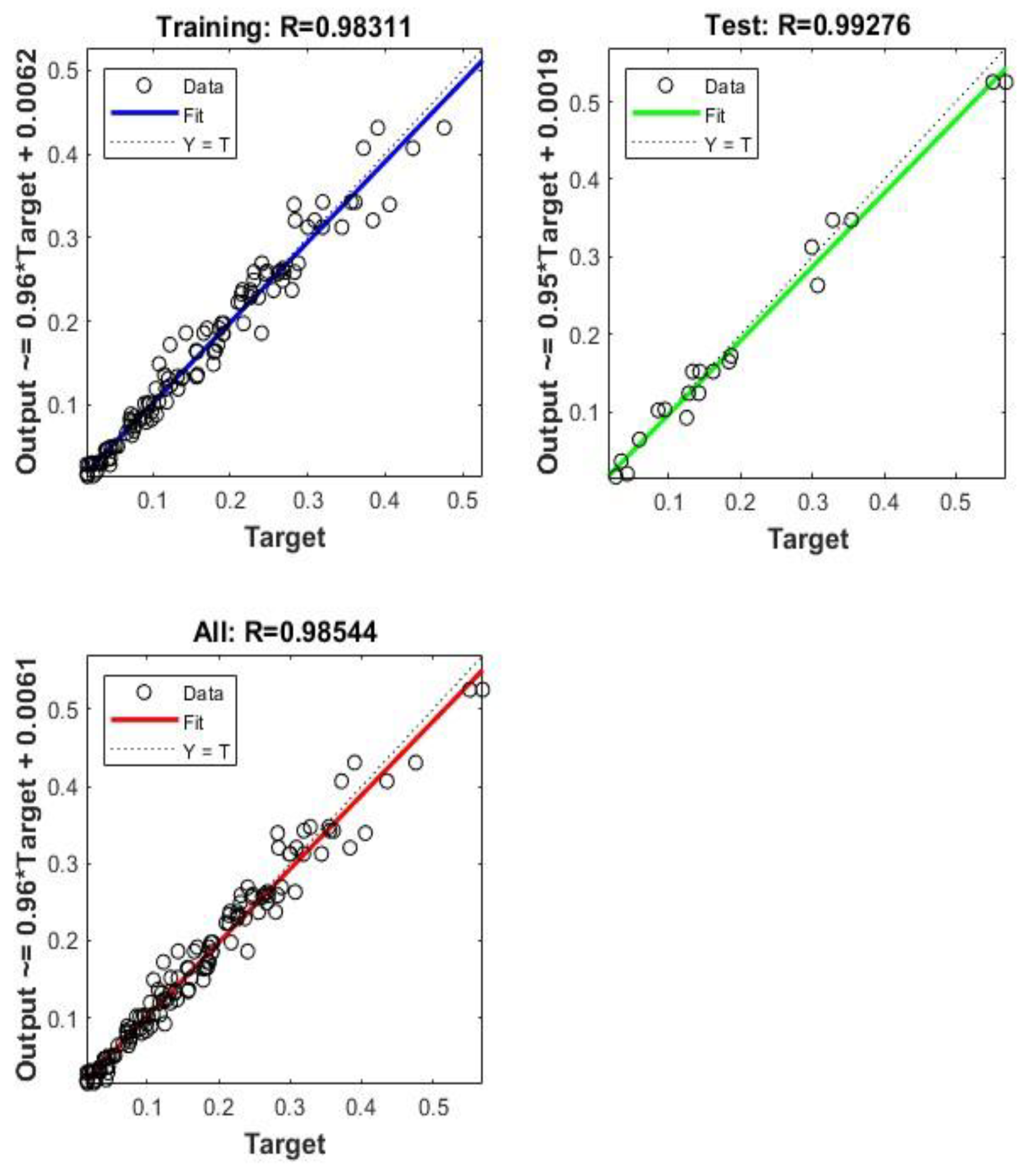
Figure 7.
Evolution of mass loss as a function of experimental and predicted values.
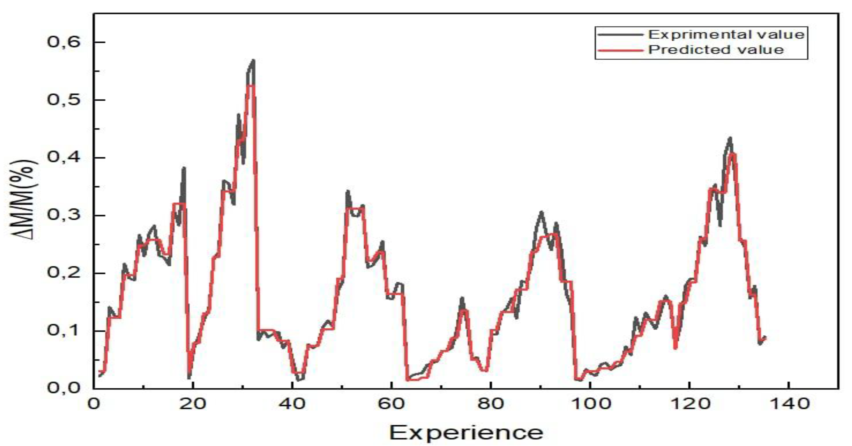
Figure 8.
Evolution of mass loss as a function of test conditions, experimental and predicted values : (a) NG24 : V = 8.3m/s, (b) NG24 : V = 4.18m/s and (c) NG12: F = 175N.
Figure 8.
Evolution of mass loss as a function of test conditions, experimental and predicted values : (a) NG24 : V = 8.3m/s, (b) NG24 : V = 4.18m/s and (c) NG12: F = 175N.
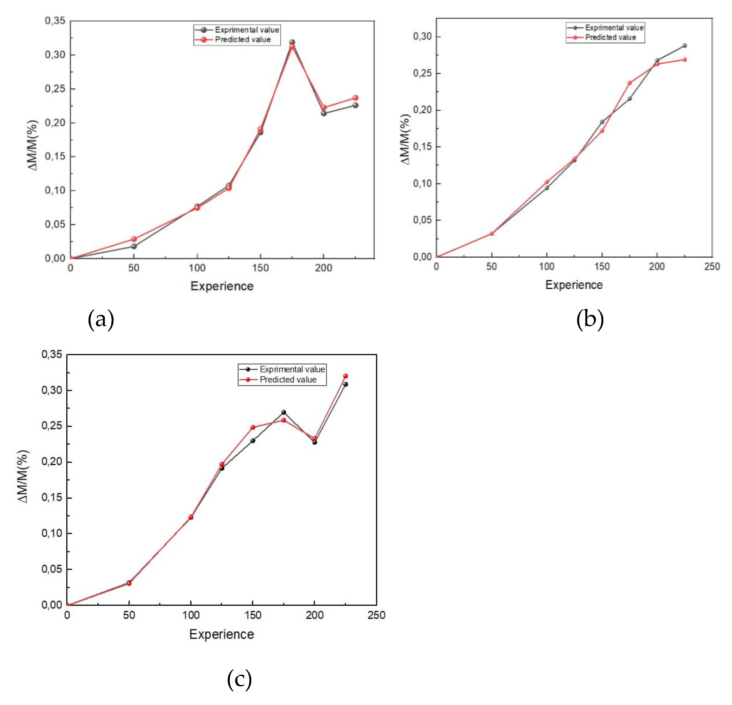
Figure 9.
Evolution of the mean square error over generations.
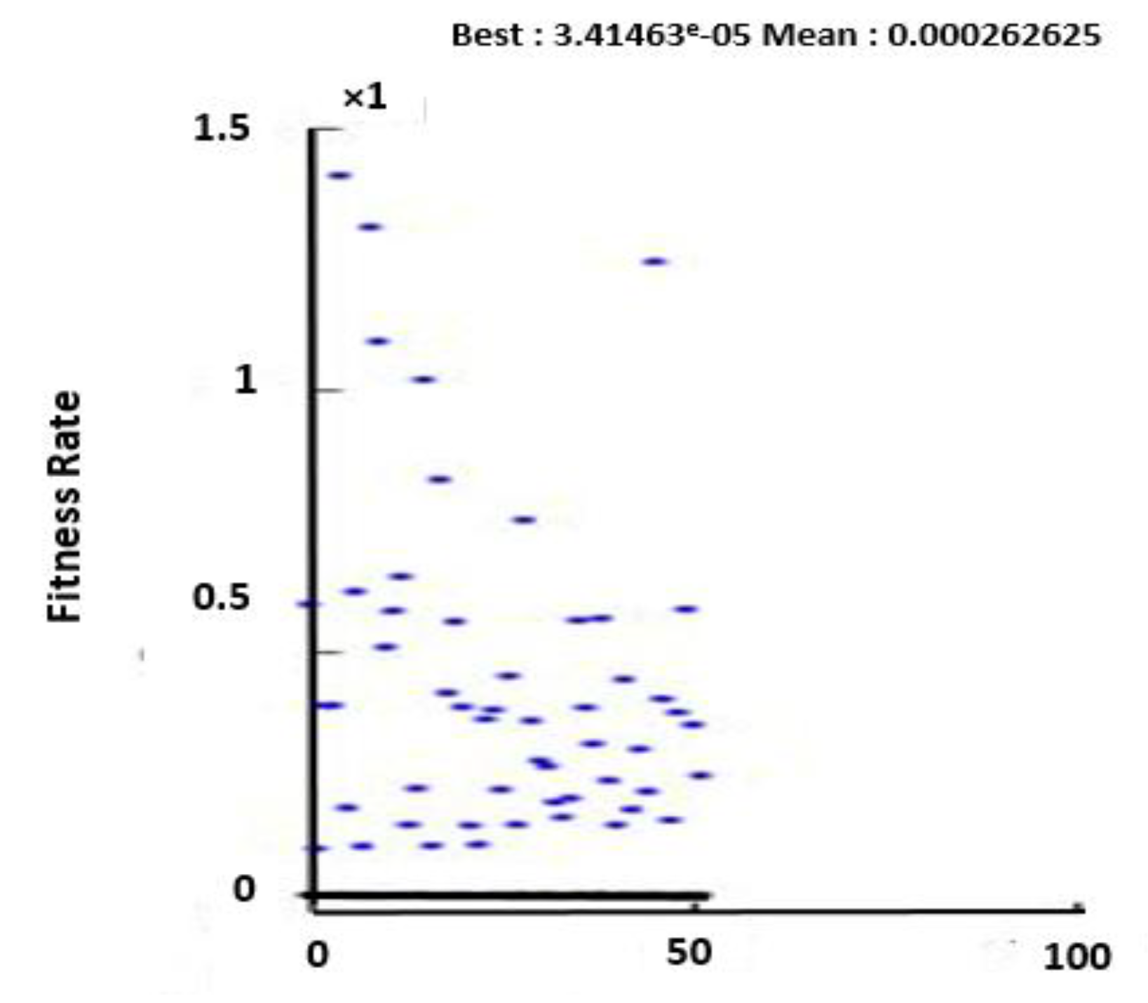
Figure 10.
Evolution of the mean square error.
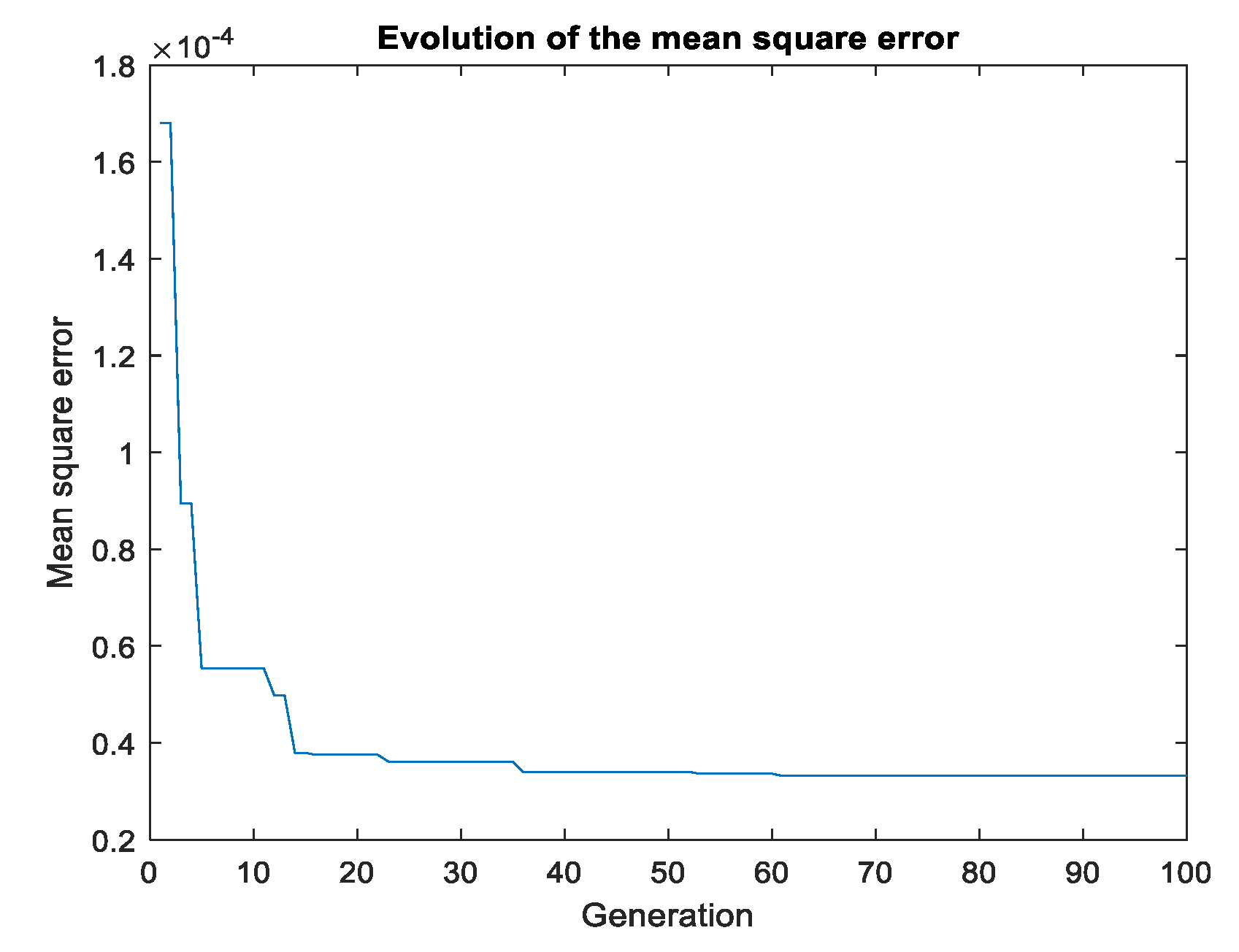

Table 1.
Chemical composition of 42CrMo4 steel.
| Elements | Cr | Mn | C | Si | Cu | Mo | Ni | S | P | Fe |
|---|---|---|---|---|---|---|---|---|---|---|
| (%) | 1.02 | 0.77 | 0.41 | 0.28 | 0.25 | 0.16 | 0.16 | 0.026 | 0.019 | Bal. |
Table 2.
Nitriding conditions and surface hardening of nitrided layers.
| State | Treatment conditions | Microhardness | ||
|---|---|---|---|---|
| θn (°C) | t (h) | τ (%) | HV | |
| NG12 |
525 |
12 |
35 |
895 |
| NG24 | 24 | 1090 | ||
| NG36 | 36 | 930 | ||
Table 3.
Information on the various Factors and levels of the wear parameter.
| Factors | Type | Levels | Values |
|---|---|---|---|
| Normal load (N) | Continuous | 4 | 100 - 125 - 150 - 175 |
| Hardness (HV) | Continuous | 3 | 895 - 930 - 1090 |
| Speed (m/s) | Continuous | 2 | 4.18 – 8.30 |
Table 4.
Neural network architecture.
| Factors | Hardness (HV) – Normal Load (N) – Speed (m/s) |
|---|---|
| Response | Mass mpss (%) |
| Activation function | Sigmoid – Hyperbolic – Linear |
| Learning algorithms | Trainlm – Trainbr – Trainscg |
| Number of layers | 1 – 2 – 3 |
| Number of neurons | 10 – 11 – 12 |
| Data report | 70 - 15 - 15 |
| Tool | Matlab 2019a |
Table 5.
Responses for raw signal ratios.
| Level | Hardness (HV) | Normal load (N) | Speed (m/s) |
|---|---|---|---|
| 1 | 14.57 | 25.34 | 24.34 |
| 2 | 22.10 | 21.71 | 16.10 |
| 3 | 24.01 | 18.48 | - |
| 4 | - | 15.36 | - |
| Delta | 9.44 | 9.98 | 8.24 |
| Rank | 2 | 1 | 3 |
Table 6.
Estimated regression coefficients, corresponding P values and variance analysis for the final regression model.
Table 6.
Estimated regression coefficients, corresponding P values and variance analysis for the final regression model.
| Source | Sum of square | df | Mean Square | F-value | P-value |
|---|---|---|---|---|---|
| Model | 0.1367 | 3 | 0.0456 | 6.84 | 0.0024 |
| A-Hardness | 0.0391 | 1 | 0.0391 | 5.87 | 0.0251 |
| B-Normal load | 0.0827 | 1 | 0.0827 | 12.40 | 0.0021 |
| C-Speed | 0.0149 | 1 | 0.0149 | 2.24 | 0.1498 |
| Residual | 0.1333 | 20 | |||
| Cor total | 0.2699 | 23 |
P < 0.01 highly significant; 0.01 <P < 0.05 significant; P > 0.05 not significant.
Table 7.
Summary of the best predictions of each activation function.
| Configuration | Results | ||||||||
|---|---|---|---|---|---|---|---|---|---|
| Activation function | Algorithms | Number of layers | Number of neurons | Training | Test | Validation | R | MSE | RMSE |
| Sigmoid | Trainlm | 1 | 12 | 0.9720 | 0.9805 | 0.9730 | 0.9721 | 0.0007 | 0.0275 |
| Trainlm | 2 | 12 | 0.9827 | 0.9816 | 0.9822 | 0.9814 | 0.0005 | 0.0022 | |
| Trainlm | 3 | 10 | 0.9854 | 0.9949 | 0.9835 | 0.9878 | 0.0004 | 0.02 | |
| Sigmoid | Trainscg | 1 | 11 | 0.9336 | 0.9795 | 0.9533 | 0,9419 | 0.0015 | 0.0398 |
| Trainscg | 2 | 10 | 0.9609 | 0.9870 | 0.9720 | 0.9649 | 0.0009 | 0.0308 | |
| Trainscg | 3 | 12 | 0.9540 | 0.9525 | 0.9818 | 0.9750 | 0.0015 | 0.0039 | |
| Sigmoid | Trainbr | 1 | 10 | 0.9836 | 0.9759 | - | 0.9843 | 0.0004 | 0.0213 |
| Trainbr | 2 | 12 | 0.9831 | 0.9927 | - | 0.9878 | 0.0003 | 0.0179 | |
| Trainbr | 3 | 10 | 0.9867 | 0.9845 | - | 0.9859 | 0.0003 | 0.0195 | |
| Hyperbolic | Trainlm | 1 | 10 | 0.9887 | 0.9810 | 0.9757 | 0.9842 | 0.0004 | 0.2147 |
| Trainlm | 2 | 12 | 0.9825 | 0.9938 | 0.9904 | 0.9839 | 0.0005 | 0.0229 | |
| Trainlm | 3 | 10 | 0.9810 | 0.9973 | 0.9947 | 0.9859 | 0.0004 | 0.0219 | |
| Hyperbolic | Trainscg | 1 | 10 | 0.9660 | 0.9573 | 0.9652 | 0.9616 | 0.0010 | 0.0318 |
| Trainscg | 2 | 12 | 0.9539 | 0.9869 | 0.9701 | 0.9596 | 0.0011 | 0.0336 | |
| Trainscg | 3 | 10 | 0.9547 | 0.9808 | 0.9815 | 0.9583 | 0.0010 | 0.0327 | |
| Hyperbolic | Trainbr | 1 | 12 | 0.9814 | 0.9731 | - | 0.9842 | 0.0004 | 0.0214 |
| Trainbr | 2 | 12 | 0.9877 | 0.9889 | - | 0.9854 | 0.0004 | 0.0200 | |
| Trainbr | 3 | 11 | 0.9852 | 0.9903 | - | 0,9859 | 0.0003 | 0.0196 | |
| Linear | Trainlm | 1 | 11 | 0.8033 | 0.8033 | 0.8033 | 0.8247 | 0.0044 | 0.02 |
| Trainlm | 2 | 11 | 0.9335 | 0.9335 | 0.9335 | 0.8433 | 0.0038 | 0.0620 | |
| Trainlm | 3 | 12 | 0.8811 | 0.8811 | 0.8811 | 0.8245 | 0.0044 | 0.0663 | |
| Linear | Trainscg | 1 | 12 | 0.8018 | 0.8018 | 0.8018 | 0.8245 | 0.0044 | 0.0039 |
| Trainscg | 2 | 12 | 0.9080 | 0.9080 | 0.9080 | 0.8345 | 0.0042 | 0.0653 | |
| Trainscg | 3 | 11 | 0.9483 | 0.9483 | 0.9483 | 0.8246 | 0.0044 | 0.0663 | |
| Linear | Trainbr | 1 | 12 | 0.8249 | 0.8249 | - | 0.8246 | 0.0044 | 0.0211 |
| Trainbr | 2 | 12 | 0.9334 | 0.9334 | - | 0.8521 | 0.0034 | 0.0529 | |
| Trainbr | 3 | 11 | 0.8249 | 0.8249 | - | 0.8501 | 0.0031 | 0.0559 | |
Table 8.
Order of trials.
| Order | Activation function | Algorithms | Number of layers | Number of neuron | R |
|---|---|---|---|---|---|
| 1 | Sigmoid | Trainlm | 1 | 10 | 0.9800 |
| 2 | Sigmoid | Trainlm | 1 | 10 | 0.9820 |
| 3 | Sigmoid | Trainlm | 1 | 10 | 0.9842 |
| 4 | Sigmoid | Trainbr | 2 | 11 | 0.9817 |
| 5 | Sigmoid | Trainbr | 2 | 11 | 0.9835 |
| 6 | Sigmoid | Trainbr | 2 | 11 | 0.9862 |
| 7 | Sigmoid | Trainscg | 3 | 12 | 0.9382 |
| 8 | Sigmoid | Trainscg | 3 | 12 | 0.9417 |
| 9 | Sigmoid | Trainscg | 3 | 12 | 0.9636 |
| 10 | Hyperbolic | Trainlm | 2 | 12 | 0.9788 |
| 11 | Hyperbolic | Trainlm | 2 | 12 | 0.9808 |
| 12 | Hyperbolic | Trainlm | 2 | 12 | 0.9814 |
| 13 | Hyperbolic | Trainbr | 3 | 10 | 0.9822 |
| 14 | Hyperbolic | Trainbr | 3 | 10 | 0.9842 |
| 15 | Hyperbolic | Trainbr | 3 | 10 | 0.9859 |
| 16 | Hyperbolic | Trainscg | 1 | 11 | 0.9215 |
| 17 | Hyperbolic | Trainscg | 1 | 11 | 0.9331 |
| 18 | Hyperbolic | Trainscg | 1 | 11 | 0.9419 |
| 19 | Linear | Trainlm | 3 | 11 | 0.8219 |
| 20 | Linear | Trainlm | 3 | 11 | 0.8232 |
| 21 | Linear | Trainlm | 3 | 11 | 0.8246 |
| 22 | Linear | Trainbr | 1 | 12 | 0.8411 |
| 23 | Linear | Trainbr | 1 | 12 | 0.8475 |
| 24 | Linear | Trainbr | 1 | 12 | 0.8495 |
| 25 | Linear | Trainscg | 2 | 10 | 0.8014 |
| 26 | Linear | Trainscg | 2 | 10 | 0.8183 |
| 27 | Linear | Trainscg | 2 | 10 | 0.8213 |
Disclaimer/Publisher’s Note: The statements, opinions and data contained in all publications are solely those of the individual author(s) and contributor(s) and not of MDPI and/or the editor(s). MDPI and/or the editor(s) disclaim responsibility for any injury to people or property resulting from any ideas, methods, instructions or products referred to in the content. |
© 2025 by the authors. Licensee MDPI, Basel, Switzerland. This article is an open access article distributed under the terms and conditions of the Creative Commons Attribution (CC BY) license (http://creativecommons.org/licenses/by/4.0/).
Copyright: This open access article is published under a Creative Commons CC BY 4.0 license, which permit the free download, distribution, and reuse, provided that the author and preprint are cited in any reuse.


