Integrated Petrophysical Evaluation and Reservoir Characterization of the Zarama Field, Offshore Niger Delta Using Multi-Well Geophysical Log Analysis

Mohammed Ali Garba; Mustafa Ali Garba

doi:10.20944/preprints202509.0568.v1

Submitted:

05 September 2025

Posted:

05 September 2025

You are already at the latest version

Abstract

In this paper, a multilateral petrophysical analysis of the Zarama field is undertaken, based on a complete set of well-wireline logs, the gamma ray, resistivity, density, and neutron logs of five wells (Wells 1-5). Emphasis is placed on important reservoir parameters, including porosity, permeability, shale volume, and fluid saturations as an effort to determine the quality of the reservoir, its heterogeneity, and producibility in the case of Agbada Formation in the Niger Delta basin. The results indicate that the reservoirs are of good and excellent porosity, with 20 to 32 percent of the reservoirs, which tends to decrease with depth due to the compaction occurrences that are dominant in offshore settings. Yet, the variation in permeability is high (7 to 781 mD), although it is more dependent on shale content (Vsh) rather than porosity as a single factor. Thicknesses of the reservoirs range between thin beds (approximately 6 m) and thick units more than 700 m, with lateral continuity being observed alongside some of the more numerous massive sands (e.g., S1, S3, S14, S16) with high hydrocarbon pore volumes and good production prospects. Interpretation of interfaces between hydrocarbon fluids, i.e., gas-water, gas-oil, and oil-water, between layers was done by integrated log analysis even in the absence of data and density log anomalies due to the presence of gas. The estimated reserves show recoverable volumes of around 2.85 million barrels of oil equivalent and 5.85 billion cubic feet of gas, which speaks to the field’s promising yield. The study highlights the fact that the gas reservoirs are dominant, with small accumulations of oil and condensate. The field is mainly gas bearing with inners of oil /condensate, as shown by the log response and neutron-density crossovers. Petrophysical ties between wells have highlighted a multi-reservoir system that is heterogeneous, but without well-defined stratigraphic trappings, and requires a multi-well exploration using integrated interpretation to allow proper characterization and reservoir development planning. The present work highlights the relevance of integrated log interpretation to address shortcomings of datasets in isolation and offers revised petrophysical parameters at a high level of confidence, as well as estimating appreciable recoverable reserves. The Zarama field shows complexities of lithological and fluid variations in the gas-dominated deltaic environment in which it is a potential offshore hydrocarbon province.

Keywords:

porosity

;

permeability

;

reservoirs

;

heterogeneity

;

gas

Subject:

Environmental and Earth Sciences - Geophysics and Geology

Introduction

Geophysical logging involves measuring a variety of subsurface physical properties—such as bulk density, porosity, water saturation, and hydrocarbon presence—by lowering a probe or sonde equipped with sensors on a wireline into a borehole (USACE, 2018). Data collected by these sensors is transmitted via a steel-armored electrical cable to surface equipment, where the information is processed and displayed as continuous well logs, showing variations of properties like spontaneous potential, resistivity, or density with depth. These measurements enable calculation and optimization of producible hydrocarbons (Ahmad et al., 20150). In addition to traditional wireline logging, (Darwin, 2008) highlighted that logging can be conducted while drilling through instruments embedded in drill collars near the drill bit—a practice known as Measurements While Drilling (MWD), Logging While Drilling (LWD), or Formation Evaluation While Drilling (FEWD). Data transmission in these cases utilizes mud pulse telemetry, where pressure pulses generated near the drill bit travel up the drilling mud and are decoded at the surface.

The Niger Delta’s modern depositional environment serves as a model for lithofacies subdivision of subsurface sequences using well logs and biofacies (Emoyan, 2008). For instance, the Upper Delta plain, a continental depositional zone, is characterized by high sand content (~80%), while transitional zones like the lower delta plain and coastal barriers have sand percentages ranging between 30-80%. Marine environments typically reflect lower sand percentages below 20-30%. Well logging technology is integral throughout exploration and production—from drilling a field’s initial wildcat well to the abandonment of its last producing zone—and has broad applications beyond hydrocarbon exploration, including groundwater and environmental investigations (Derek, 2006). Advances in logging now allow measurement of numerous physical properties in both open and cased holes, aiding in determining formation dip and the orientation of tilted strata (Benson and Kurt1998).

The significant advancements in petrophysical modeling of the Zagros region have integrated diverse datasets and employed probabilistic methods to better understand reservoir heterogeneity. However, a notable research gap remains in the limited availability and comprehensiveness of datasets, especially regarding shale content and geological complexity, which hampers the generalizability and accuracy of reservoir characterization. (Mehdi and Pooria, 2025). The comprehensive understanding of petrophysical properties in the Sapphire wells, particularly regarding the variability in porosity, permeability, and shale content derived from gamma-ray and neutron logs. Despite detailed lithological and reservoir classifications, limited data on the spatial heterogeneity of these properties and their influence on fluid flow and hydrocarbon potential hinder accurate reservoir characterization and development planning. (Naiem, et al., 2025). Hina (2024) demonstrates that integrating advanced well-log interpretation with geological and petrophysical data significantly improves the accuracy of reservoir characterization and hydrocarbon assessment. Despite extensive use of well-log interpretation for reservoir evaluation and petrophysical characterization, a significant research gap remains in developing integrated, advanced models that accurately incorporate geological, geophysical, and petrophysical data to address uncertainties in complex reservoirs. Current methodologies often struggle to fully account for heterogeneity, fluid effects, and data inconsistencies, which can lead to inaccuracies in estimating reservoir quality and hydrocarbon potential.

Geophysical well logging is the geophysical tool that is crucial during the exploration and assessment of hydrocarbon reservoirs. Well logs generate detailed and continuous data concerning lithology of rocks, porosity, fluid content, and quality of the reservoir by estimating a number of physical properties of subsurface formations, including resistivity, density, neutron porosity, and acoustic transit time. These results are very essential in identifying the presence or producibility of hydrocarbons within a field. Niger Delta is one of the most prolific hydrocarbon basins in Africa with complex stratigraphy that comprises sand to shale beds, mainly that of the Agbada Formation. Gathering the idea about the petrophysical properties of these rocks: Porosity, permeability, saturation levels of water, and the volume percentage of shale, is essential to characterize the reservoir effectively and extract the maximum amount of hydrocarbons. This is a paper about the field of Zarama of the Niger Delta, where they use 5 wells as a case to study well logs and develop important reservoir parameters. The investigation intends to differentiate the reservoir units, determine approximations of the fluid saturations, and evaluate the level of quality of the reservoir by incorporating various measurements of logging measurements. In addition, the paper assesses fluid contacts and estimates recoverable reserves, giving a really important idea of the production potential of the field and where the future development should be aimed at. Although the comprehensive petrophysical reviews of the Zarama field have been carried out, a number of challenges and limitations affected the data analysis and interpretation. Another problem was the existence of unreliable density logs, especially in Well-1, in which the density measurements in shallow intervals showed an unrealistic result (up to 100 g/cc) associated with an effect of the gas or an error in the calibration of the tool. Such anomalies required specific data employed, where in some cases only resistivity logs were used, and this could conceivably add ambiguity to estimates of porosity and fluid saturation. The other weakness was that some details on logs coverage were left uncovered in certain wells, like gamma situations or neutrons used in Wells 3, 4, with lithology and porosity adjustments having insufficient confidence in such areas.

Also, deep lithological stratigraphic heterogeneity and finely stratified sands and lateral discontinuity between wells, when found, hampered the correlation of reservoir units and mapping of fluid contacts that could affect volumetric calculation of reserves. The interpretation of the type of fluid using neutron-density crossovers and resistivity also gave rise to difficulty in the differentiation of gas and oil or water in zones where logs attested to be shifted as a result of borehole conditions or invasion results. In addition, there is an absence of core data that can be used to directly calibrate petrophysical parameters, therefore impeding the validation of logging datum, but the region analogs were used to give a point of calibration. Broadly adopted empirical equations that are employed to estimate the permeability inherently share this supposition based on average-grain size and sorting impacts, they may not be adequate to describe entire ranges of reservoir quality throughout the field. Future research and developments will have to cover areas of improving reservoir characterization by integrating solutions such as higher-resolution log acquisition, core analysis, and advanced petrophysical modeling together in order to minimize uncertainties and subsequently enhance the accuracy of reservoir characterization in the future. Petrophysical analysis of the Zarama field in the Niger delta was based on well logs of the five wells, and interpretation of gamma ray, resistivity, density, and neutron logs were factors considered in specifying the reservoir characteristics.

Method and Materials

To conduct a logging operation, a probe or sonde is lowered into the well on an insulated electrical cable, which supplies power and transmits sensor data back to the surface. Depth is measured via the cable. Data is processed and plotted both analog and digitally. While most logs are recorded during pull-out, some methods like MWD, LWD, and flow meter logging occur during descent. Logging tools include gamma ray, resistivity, density, neutron, and sonic, among others.

Resistivity Logging: Evaluation of fluid content in oil and water wells uses electrical resistivity to identify water or hydrocarbons by measuring ion flow through pore fluids. Higher resistivity suggests better water quality or more hydrocarbons, while lower values indicate saline water. Resistivity at different depths, obtained by varying electrode spacing, helps detect invasion zones and permeability, influenced by factors like salt concentration, temperature, and porosity.

F = \frac{R_{0}}{R_{w}}

(1)

where Ra is the resistivity of a 100 percent water-filled formation, and Rw is the resistivity of the water.

Formation Resistivity Factor: Formation Resistivity Factor (F), the ratio of resistivity in a fully water-saturated formation (Ra) to that of formation water (Rw), aids interpretation of measurements. Electric logging tools apply voltage between electrodes, causing current flow in formation fluids. The resulting voltage reflects formation resistivity, with electrode spacing determining investigation depth. Short and long spacings provide shallow and deep resistivity data vital for evaluating reservoir fluid type, characteristics, and permeability for exploration and production.

Acoustic Logging: An Acoustic Log, or sonic log, provides valuable information on the physical structure of rock matrices using tools such as the long-spacing sonic tool, a slender version for tubing installations, and the borehole-compensated tool. These instruments consist of transmitter and receiver transducers that convert electrical energy to mechanical energy and vice versa. The borehole-compensated tool measures two At values from multiple receivers, averaging them to eliminate errors from sonde tilt and borehole size variations (Crane, 1986). Since transit time includes borehole fluid and formation travel, Geoffrey and Stephen (2011) recommend subtracting borehole transit time. Acoustic logs reveal transit time (density) and amplitude (interconnections) and also demonstrate that At relates to porosity and is defined bulk velocity as the sum of fluid and matrix velocities, with the relation between bulk velocity (Vb) and fluid velocity (Vf) described by Willy’s equation.

\frac{1}{V_{b}} = \frac{f}{V_{r}} + \frac{1 - f}{V_{m a}}

(2)

The equation for porosity (Ɵ) obtained from transit time (Δt) (which is the reciprocal of velocity) is:

θ = \frac{Δ t_{l o g} - Δ t_{m a}}{Δ t_{f} - Δ t_{m a}}

(3)

where Δt_log = measured transit time, Δt_f = fluid time transit, and Δt_ma = assumed matrix transit time.

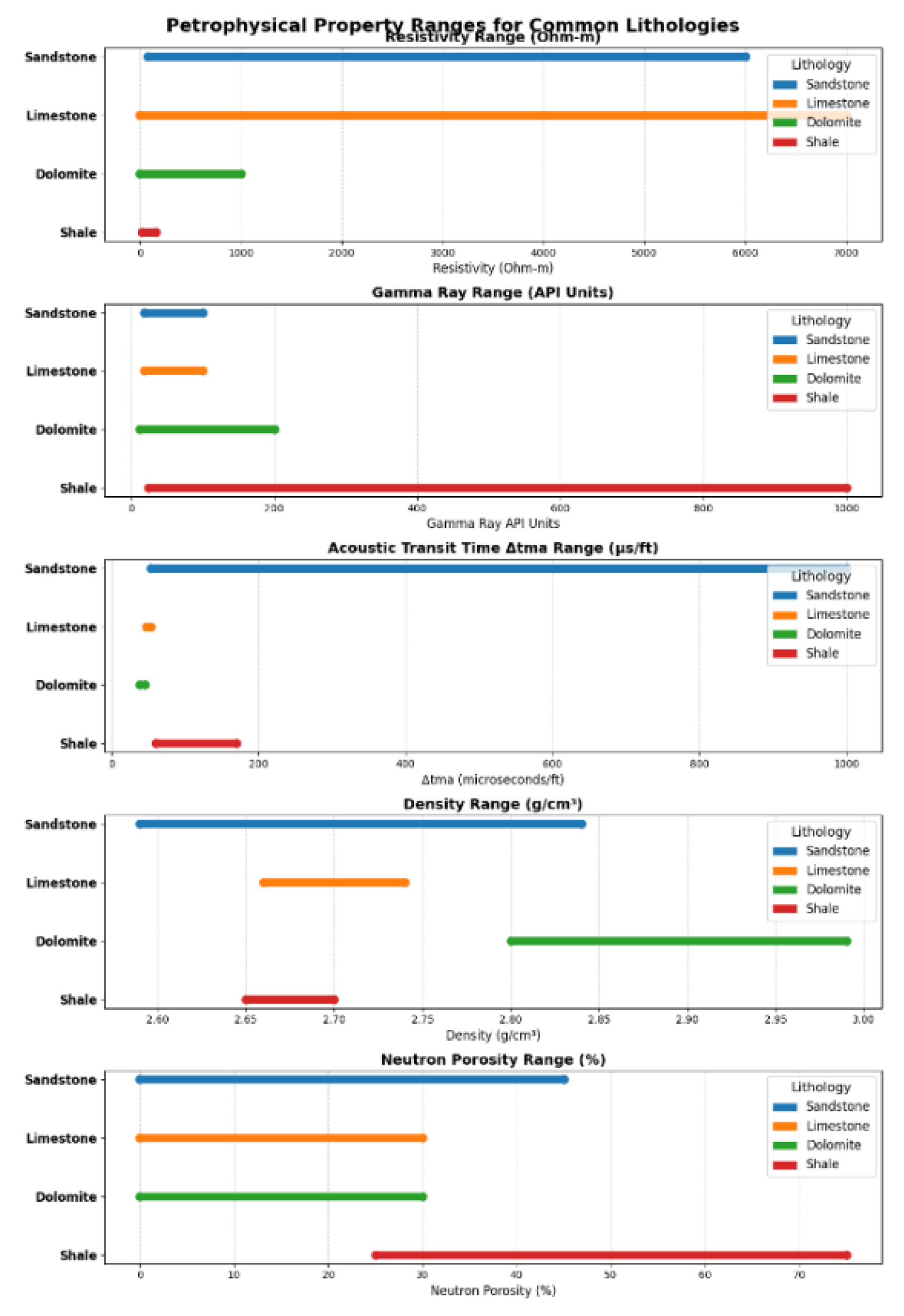
Figure 1. Petrophysical Property Ranges for Common Lithologies.

Neutron Logging: A neutron log measures formation porosity around a borehole by detecting hydrogen atoms through gamma rays emitted when high-energy neutrons, from sources like Plutonium or Beryllium, collide with hydrogen nuclei, losing energy. Thermalized neutrons are captured by nuclei, emitting detectable gamma rays. High hydrogen concentration near the borehole traps neutrons, resulting in lower gamma counts indicative of high porosity, while low hydrogen areas allow neutrons to travel further, generating higher counts and low porosity. Non-porous, dense rocks (e.g., limestone) show high counts, while shale, rich in bound water, has low counts despite low porosity, complicating lithology interpretation without supporting logs. Neutron logs function in various borehole fluids, aid correlation with gamma-ray or casing locator logs, and detect gas presence and movement due to hydrogen density changes, proving valuable for production logging and fluid dynamics analysis.

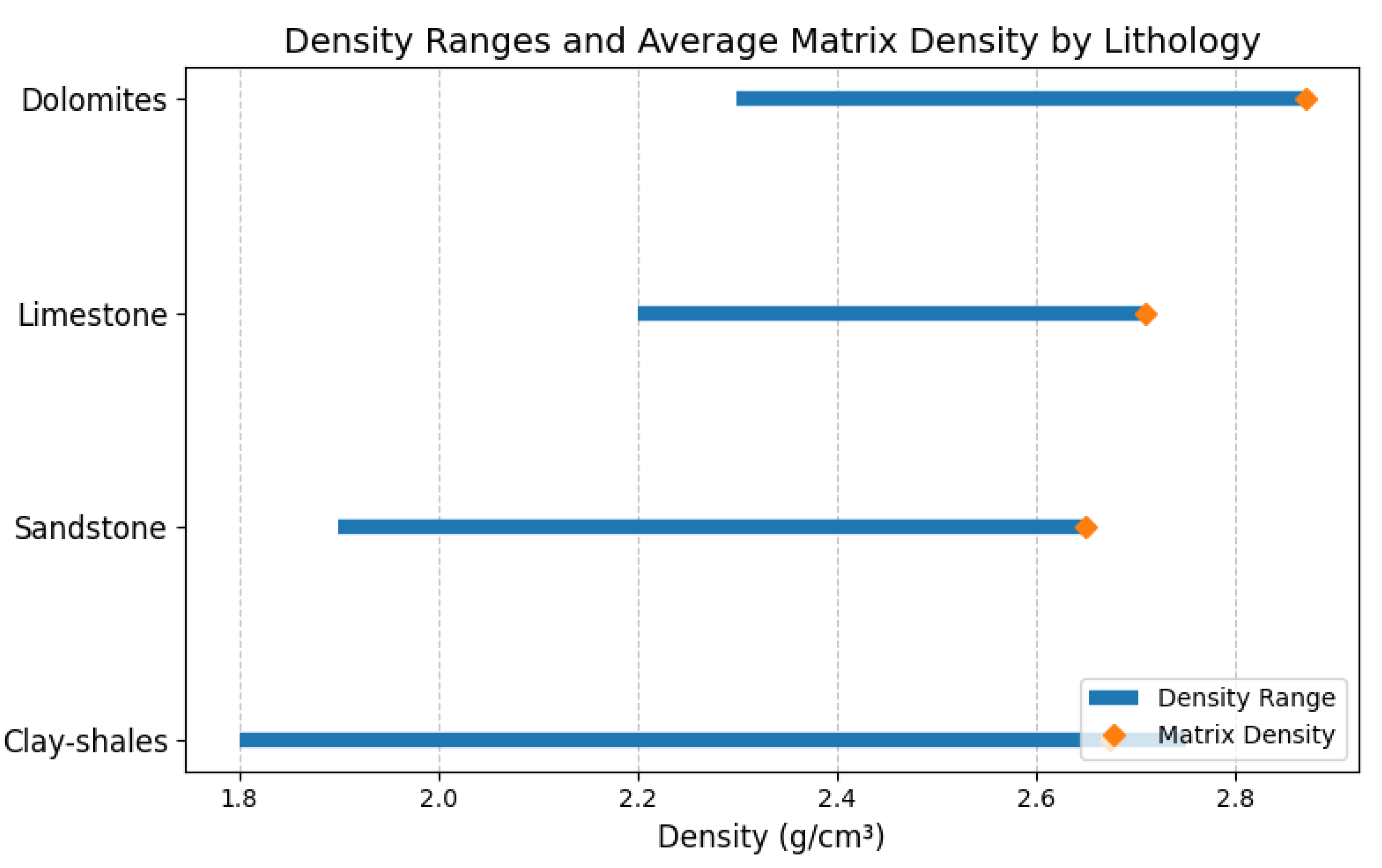
Density Logging: Density logging tools measure the bulk density of formations within a wellbore using a dense metal mandrel that collimates backscattered gamma rays. A caliper ensures proximity to the wellbore wall for accurate measurements. The instrument includes a scintillation detector, typically a sodium iodide crystal, which converts gamma rays into light photons, then into electrons within a photomultiplier tube. These electrons are amplified through dynodes, producing pulses proportional to the detected gamma rays. Analysis of these signals yields the formation bulk density essential for porosity and lithology determination. Merritt (2007) demonstrated that backscattered gamma counts correlate with electron density, closely linked to bulk density via the Z/A ratio (~0.5) for lightest elements.

δ_{e} = δ_{b} (2 \frac{Z}{A})

(4)

where σ = bulk density, o = electron density, Z-sum of the electrons, A total Atomic weight.

Crane (1986) and Kane and Lucia (2004) showed a direct relationship between formation bulk density and porosity (0), fluid density, and matrix density of the rock material, bulk density (a) being the sum of the fluid density (a) of the pore space and the density of the matrix (Gm) (Table 1 and Table 2).

δ_{b} = ϕ . δ_{f} + (1 - ϕ) . δ_{m n}

(5)

Rearranging the equation,

Φ = \frac{σ_{m a} - σ_{b}}{σ_{m a} - σ_{f}}

(6)

Porosity (0) can be calculated given bulk density (os), and if fluid density (or) and matrix density (...) are known. The densities of some lithologies are shown in Table 1. Typical fluid density (ρd) of water is 1.0 g/cc. Formation fluids containing oil and gas 0.7 g/cc. Formation fluids containing gas 0.3 g/cc.

Gamma Ray Logging: Natural gamma radiation varies in rock formations due to the presence of radioactive minerals such as Uranium, Thorium, and Potassium, which are associated with distinct depositional environments. Sedimentary sandstones and carbonates typically exhibit low gamma radiation, while clay and shale formations have higher gamma radiation levels (Crane, 1986). Gamma ray logs, recorded in counts or API units, help identify lithology based on count rates, with clean sands showing low counts and shaly formations exhibiting higher counts (Geauner et al., 2004). Higher gamma counts correlate with clay-rich, more compacted formations that possess reduced porosity and permeability (Crane, 2006; Merritt, 2007). Odom (2002) noted that formations with high gamma counts are generally less favorable for oil and water production, despite possibly low water saturation. The gamma ray tool uses a scintillation detector, usually a sodium iodide crystal, where gamma rays produce light flashes converted into electrical pulses proportional to retained gamma energy after collisions. Besides identifying shale intervals, gamma ray logs estimate shale volume, a crucial parameter to adjust other log measurements for clay effects during reservoir evaluation. Table 2 and Figure 2.

Data Analysis

The dataset for this study comprises geophysical logs—including gamma ray, resistivity, density, and neutron logs—collected from five wells within the Zarama field, supplied by Shell Petroleum Development Company of Nigeria Limited (SPDC) in Port Harcourt, Nigeria. These logs were obtained using standard wireline logging methods, with density-neutron and gamma-ray measurements recorded by a single tool, and resistivity acquired via a separate instrument. Reservoir petrophysics involves measuring well data, processing it, and integrating these results into physical models that describe the reservoir rock at both the well and field scales. This includes calculating and interpreting key reservoir properties and correlating them with data from core samples, tests, and production to characterize the reservoir accurately. According to Coates (1995), essential petrophysical properties for assessing hydrocarbon producibility are porosity, permeability, and water saturation (S_w), the fraction of pore space filled with formation water. Porosity fully saturated with water (S_w = 100%) is not viable for oil production, linking S_w to bulk-volume water (B), the percentage of total formation volume made up of water, by:

B_{v w = ϕ S_{w}}

(7)

Given the critical importance of the S, as discussed above, many techniques have been proposed for determining its value for a given formation (Berg, 1995). In log interpretation, the standard approach to water saturation is through the Archie formation factor process, defined by

F = \frac{R_{0}}{R_{w}} = \frac{C_{w}}{C_{0}}

(8)

The resistivity of a reservoir rock fully saturated with an aqueous electrolyte is related to the electrolyte’s resistivity, with their corresponding conductivities linked accordingly. Using porosity (φ) and resistivity (R), Archie’s formation factor analysis provides empirical relationships connecting porosity to formation factor and resistivity to water saturation (S). Petrophysical information on the Zarama field is limited, so this study uses well log data to evaluate reservoir producibility and estimate reserves. Wireline logs from five wells reveal the Agbada Formation’s alternating sand and shale sequences, with key reservoir properties like porosity (20–32%), permeability (7–781 mD), and shale volume derived from gamma-ray, resistivity, density, and neutron logs. Fluid contacts such as gas-water and oil-water were identified, with gas predominating. Despite challenges like inconsistent density logs in gas zones, integrated log analysis enabled reliable mapping of reservoir heterogeneity, thickness variations, fluid saturations, and promising recoverable reserves due to well-developed hydrocarbon traps Figure 3.

Petrophysical Data Analysis

The obtained raw data were plotted into well log signatures using an Excel spreadsheet on a linear scale (gamma ray, density, and neutron logs) and a logarithmic scale (resistivity log) for each of the five wells, with gamma-ray log on track 1 and resistivity, density or neutron logs on tracks 2 and 3 for the same depth. In wells 1 and 5, the resistivity log was placed on track 1 for the absence of gamma-ray log and density and/or neutron logs on tracks 2 and 3 as applicable.

Shale Volume: The gamma-ray index option was employed to determine shale volume and, implicitly, the dominant lithology. This was achieved by determining the clean sand line on gamma-ray logs. A correction was made to the gamma-ray index to compensate for the unconsolidated sand of the Niger Delta. The volume of shale was calculated using the equation below, following Crane (2006), Merritt (2007), and Ruhn (2007) relations. The

The parameter also served as input data in the porosity and saturation model for shaly sand.

V_{s h} = 0.33 (2^{2.1 G R)} - 1.0)

(9)

where

V_{s h}

= shale volume

and

I_{G R} = \frac{G - G_{c s}}{G_{s h} - G_{c s}}

(10)

G = gamma ray reading in the zone of interest

G_{c s}

= gamma ray reading in clean sand and

G_{s h}

= gamma ray reading in shale zones.

In wells 1 and 5, shale volumes, Vsh, were computed using Henderson (2007) expression:

V_{s h} = [\frac{R_{s h} (R_{c s} - R_{t})}{R_{t} (R_{m s h} - R_{s h})}]

(11)

where

R_{s h}

is the resistivity of 100% shale formation,

R_{c s}

is the resistivity of clean sand,

R_{t}

is true resistivity, and

R_{m s h}

is the maximum resistivity in the shale pay interval.

Porosity: Reservoir porosities were computed from density logs using the expression after Crane (1986), Comisky (2002), Merritt (2005), and Ruhn (2007).

ϕ_{d} = \frac{ρ_{m} - ρ_{b}}{ρ_{m} - ρ_{r}}

(12)

Neutron porosities (0) were read directly from neutron logs. The porosities were corrected for shale using the expression (Aigbedion and Iyayi, 2007).

ϕ_{d} = \frac{ρ_{m} - ρ_{b}}{ρ_{m} - ρ_{r}} - \frac{ρ_{m} - ρ_{b}}{ρ_{m} - ρ_{s h}} V_{s h}

(13)

where p is the density of adjacent shale

The porosities from density and neutron logs in well 5 were integrated to obtain equivalent porosities (0) using Gemini (2002) relations:

ϕ_{e} = \sqrt{\frac{ϕ_{n}^{2} + ϕ_{d}^{2}}{2}}

(14)

Formation resistivity factor, F, was determined using Archie’s (1942) equation.

F = \frac{1}{ϕ^{m}}

(15)

where a is the cementation constant, and m is the cementation factor. Cementation constant, a=1 was used in this study, and the cementation factor, m, in the Niger Delta was reported by Kofron et al. (1996) and Aigbedion (2006) to be 1.8. The value of m 1.8 was used in this study.

Water and hydrocarbon saturations: Water and hydrocarbon saturations are usually estimated from the well logs using. Archie (1942) saturation equation.

S_{w} = [\frac{R_{0}}{R_{t}}]

(16)

S_{h} = 1 - S_{w}

(17)

where

S_{w}

is water saturation

R_{0}

= resistivity of 100% water-filled formation

R_{t}

= true resistivity

n = saturation exponent

S_{h}

hydrocarbon saturation

Reformation water resistivity

Saturation exponent, n = 2, was used in this study. However, R could not be directly determined from the available deep resistivity logs, so Henderson’s (2007) relations for water saturation, S., were used as follows.

S_{w} = [\frac{R_{n s} . 10^{Y t}}{R_{t}}] 1 / n = [\frac{R_{n s} . 10^{Y t}}{R_{t}}] 1 / 2

(18)

where

. 10^{Y t} = R_{0} a n d R_{n s}

is the resistivity of non-source shale and

Y_{t}

is defined by

Y_{t} = l o g_{10 [\frac{R}{R_{n s}}]}

(19)

Permeability Permeability was estimated from porosity and Vsh using the formula (Comisky 2002):

K = 10^{[A + B l o g (ϕ) + C V}

(20)

where A, B, and C are constants defined as follows:

A = 7.432; B=8.060; and C = -5.508

This equation takes into account grain size and sorting through the Vsh (shale content) term, and the grain size and sorting have a significant effect on permeability (Timur, 1968; Vernik and Nur, 1992; Coates, 1995; Vernik, 2000; Comisky, 2002; Pelechaty et al.,2005). From the petrophysical properties and/or parameters evaluated from the well logs from each of the wells, reservoir components- water, oil, and gas were identified, and their contacts (gas-oil-contact- GOC; oil-water-contact-OWC; gas-water-contact-GWC; gas-down-to-shale-GDT; and oil-down-to-shale-ODT) were established and net pay computed.

Reserve Estimate: Hydrocarbon pore volume (HCPV) under reservoir conditions was estimated empirically as a function of the reservoir rock and fluid properties following Ojo’s (1996) standard volumetric equation.

H C P V = A H N G x θ x S_{h}

(21)

where A is the area enclosed by a trap, It is the gross reservoir thickness, N/G is the net-to-gross reservoir thickness relationship. O is the porosity, and S is the hydrocarbon saturation.

The recoverable reserve was estimated using the expression after Rondeel (2002)

R_{e} = (H C P V \times R_{i}) / F_{v}

(22)

Where Re is the recoverable reserve, Rr is the recovery factor, and Fvf is the formation volume factor. It has been generally reported (Opara, 1981), and accepted (Ojo, 1996), that only 45% of reserves are recoverable, and 1.4 has been used as formation volume factor in the Unam B field in the Niger Delta. In this work, the recovery factor (Rr) was taken as 45% and

F_{v i} = 1.4 .

Fluid detection

Gas-Bearing Formations: Gas-bearing zones were delineated where apparent density is decreased (since gas contains less dense fluids). The relationship between electron density (which is normally measured by the tool) and bulk density is somewhat different for gas than for a rock containing oil or water. The combined effect is an increase in density porosity, implying a decrease in bulk density reading. The neutron porosity in the zone should show a decreased value because the formation contains less hydrogen per unit volume, and the tool equates porosity with the amount of hydrogen in the formation. Hence, the combination of these two effects results in the density/neutron separation. The zone was detected with an increased resistivity response. A combination of two or more of these log behaviours was used to detect gas-bearing zones.

Oil-Bearing Formations: Oil-bearing zones were detected when the density/neutron curves tend to track together (come together), with evidence of moderate resistivity, and where the density log shows an average reading and the resistivity log shows a much lower reading than that of gas-bearing zones. Hydrogen ions in oil and water-bearing formations are almost the same, but the hydrogen ions in oil-bearing formations are far more resistant than in water-bearing formations. So resistivity in formations containing oil is far higher than resistivity in brine. Also, brine does not have much pronounced effect on the density reading, but in oil-bearing formations density reading is lower because brine/water is denser than oil.

Water-Bearing Formations: The neutron porosity is formulated by assuming a water-bearing limestone matrix. Since the reservoir lithology in the Niger Delta is predominantly sandstone, the sandstone-compatible scales were used for the density and/or neutron logs. In this regard, water-bearing zones were delineated where the density and neutron curves practically overlay each other (that is, an interplay) over the whole porosity range. The resistivity curve for the same zone should indicate a highly conductive zone (low resistivity). The density log records a high reading as water is denser than hydrocarbons. Observations from relevant logs in the field under study reveal responses as described above in water-bearing zones. Departures between these two curves (that is, density and neutron logs overlaying each other) were used to infer that the lithology or fluid content does not correspond to that of water-bearing sand.

Results

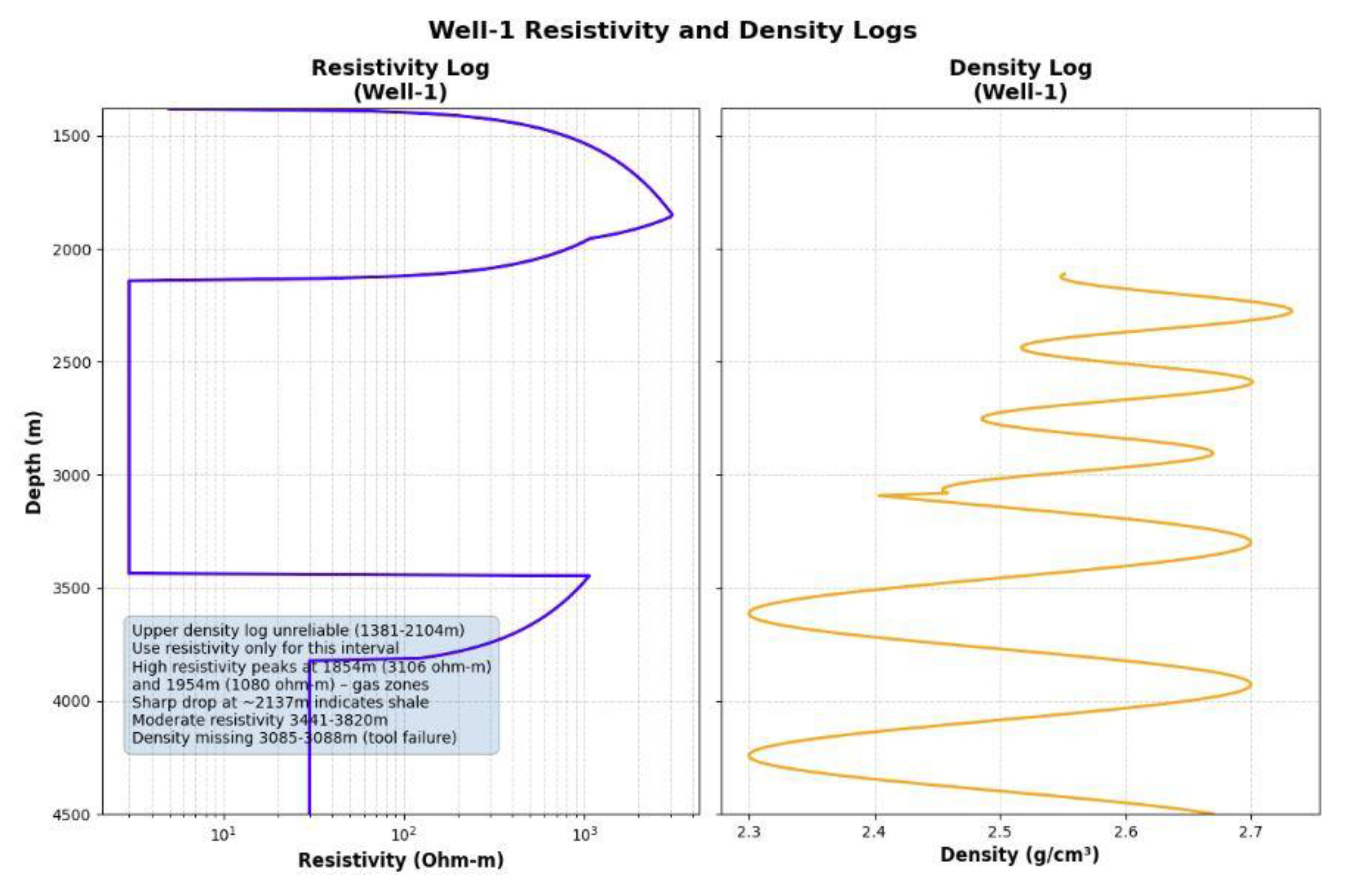
Well-1: Well-1 has a density log and a resistivity log. But the top part of the density log of the range 1381 to 2104 meters was omitted in interpreting since it had unclear scaling and the values ranged up to 100g/cc- making it unrealistic with respect to lateral sand and shale deposits of the underground. Therefore, the interpretation of petrophysical studies in this range was based on the resistivity log only. Under this depth, resistivity and density logs were also added to the assessment. The resistivity values are very high as recorded in the 1384 to 2095 meter reservoir, which is soaring at 3106 ohm-m at 1854 meter and 1080 ohm-m at 6410 meter. Such high resistivity measurements are arguably to be blamed on the presence of gas and not on under-compaction, as this is deemed unlikely at a depth of approximately 2000 meters. At around 2137 meters, resistivity is reduced to almost 1.52 ohm-m, indicating a shale layer. The formations demonstrated a strongly resistive nature between 3441-3820 m; still, the values are reduced when compared to the upper reservoir section. The density log above about 2104 meters was considered unreliable, and it was reported that the unreliability may have been because of calibration problems with the density reading being abnormally low, due to gas effects. Below 2104 m, the density is typical of the usual variations within sand and shale sequences as recorded in the density log. Remarkably, values of density are absent within 3085 and 3088 meters, and that could be caused by a malfunction of the instrument or at a time when logging runs were not combined (Figure 4).

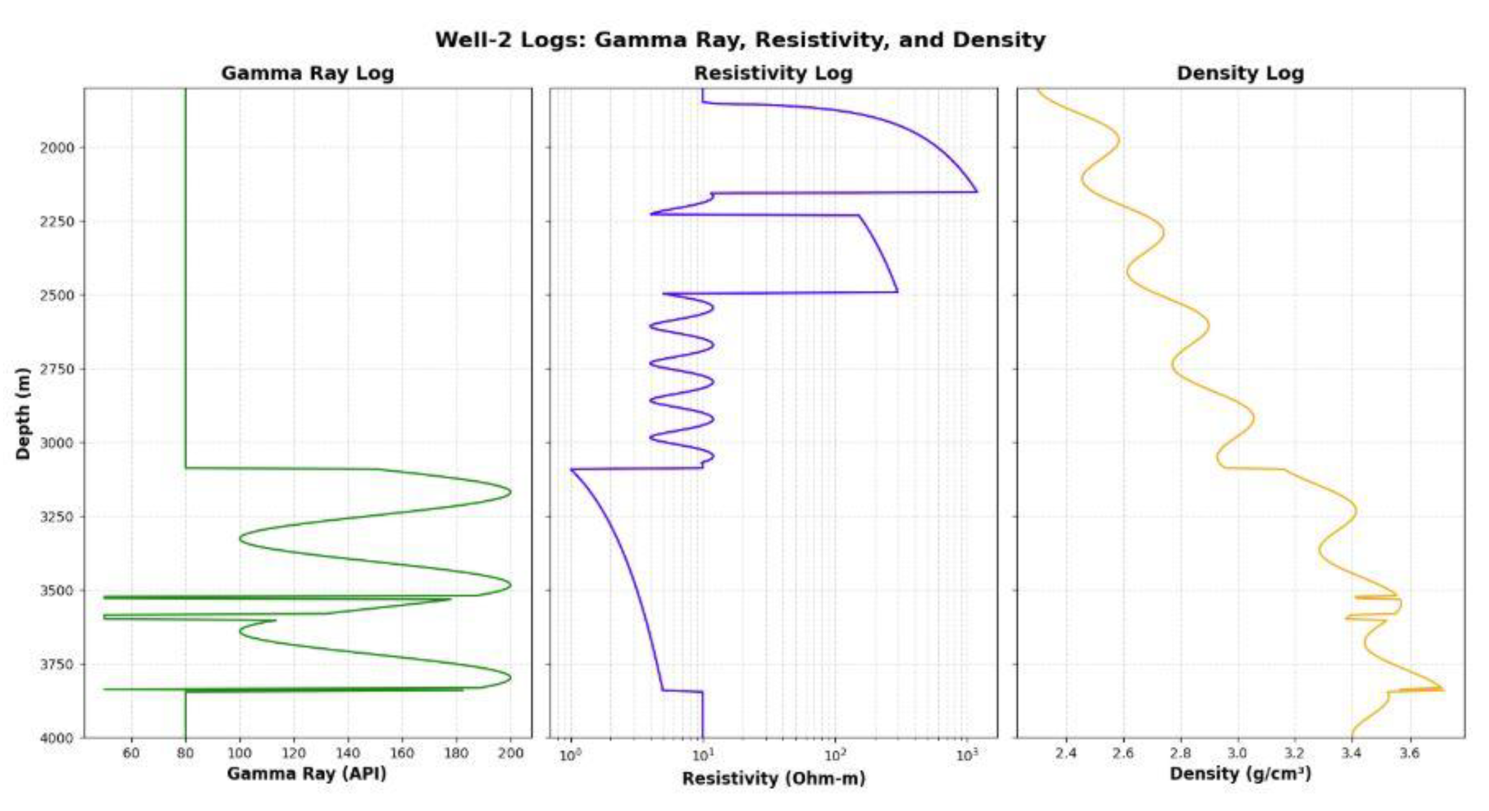
Well-2: Well-2 has gamma-ray, resistivity, and density logs. Figure 1 shows that at the logging interval, starting low at 3091 meters, a thick shale formation is seen to extend to 3845 meters with sand streaks at 3835-3838 m, 3585-3600 m, 3522-3529 m, and 3225-3227 m. The support given by the density log is by registering high values of the density, supporting the existence of the thick shale. In the range of 1851 to 3070 meters, there is alternation of sand and shale, and above them is thick sand which records very high resistivity values, especially right up to about 2155 meters. These high values of resistivity are a good indication that there is a possibility of having gas. Reservoirs within the range of 2229 to 2494 meters exhibit middle resistivity, which indicates the presence of liquid hydrocarbons, although the density log through this section shows low sand values as compared to an average seen throughout the logged area, indicating that the liquid hydrocarbons may be the condensate. The density log shows a compaction pattern, which is common throughout the whole range of depth; the density becomes stronger with depth (Figure 5).

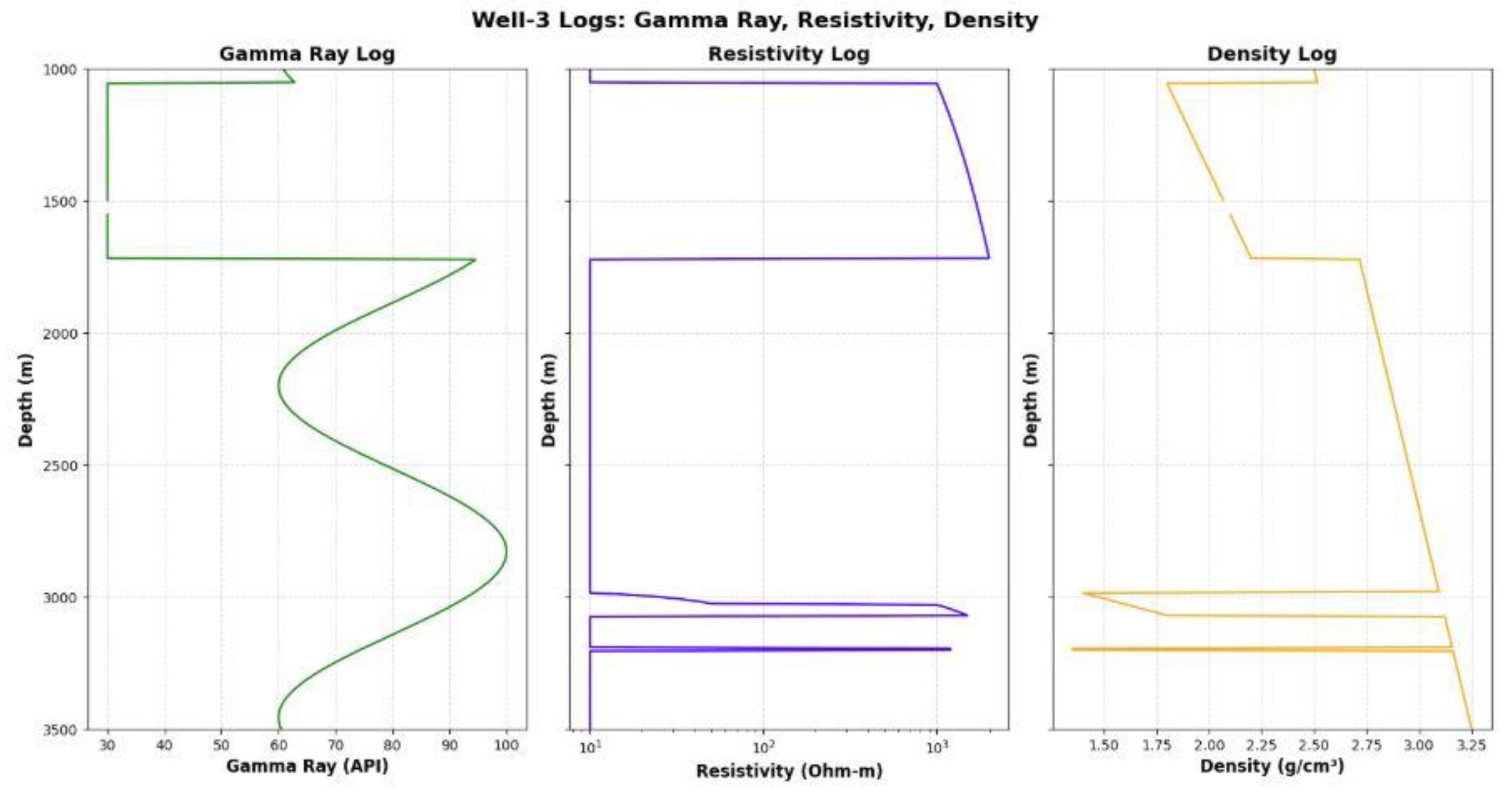
Well-3: Like Well-2, Well-3 has gamma ray, resistivity, and density logs. The upper one, 1052-1720m, is made of sand with extremely high values of resistivity and low values of density. At around 1524 meters, no data on gamma rays and density are present. The reservoirs lying between 2983-3073 meters and 3190-3204 meters show very high resistivity levels that are almost similar to the top sands reservoir level, which implies the presence of gas. The first tank (2983 3073 m) has a clear gas-water contact, most of the first half of the reservoir has very low resistivity, and at the top is a high resistivity zone. Moreover, the values of very low density are observed in this reservoir, and they are clipped because of the scale of plotting. In Well-3, these low-density zones in the two reservoirs are the only ones, with the density typically getting higher as the depth increases (Figure 6).

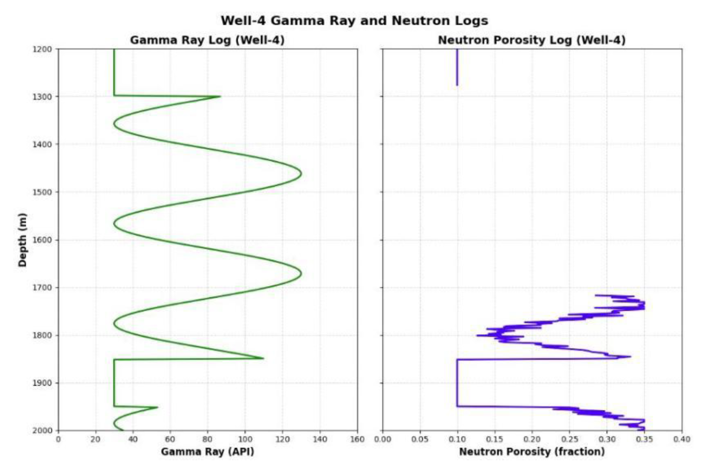
Well-4: Well-4 has gamma ray and neutron logs. Porosity for this well was read directly from the log and corrected for gas and shale effects. The top and bottom of the well have thick sand with little shale intercalations. Their neutron porosity tools reading were also low. In the upper part, 1277-1716 m, the neutron log has no data (Figure 7).

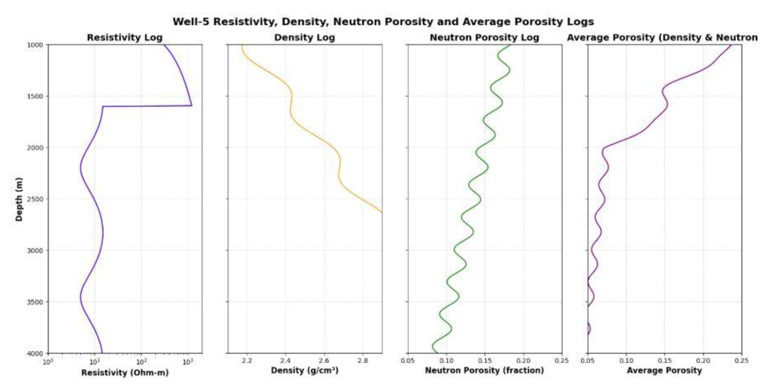
Well-5: Well-5 has resistivity, density, and neutron logs, and the upper part of the sand reservoir of this well shows high values of resistivity, just as in the other wells. The density logs show a normal compaction trend, which is, it increases with depth. An average of the porosity that was estimated using both the density log and the neutron log was used to give the porosity measurements on this well. Figure 11, Figure 12, Figure 13, Figure 14 and Figure 15 show the information about the well log data. On the basis of these logs, the lithologies interpreted are mostly the layering of sand and shales that dominate the Agbada Formation. Table 3 presents the reservoirs that are observed in all wells and referred to as sands 1 to 16 simply because it is convenient to do so, and the results of the petrophysical analysis. Both wells had relatively continuous and highly permeable sand formations of thick nature down to a depth of 7010 feet (2137 meters) in Well-2 and 6770 feet (2064 meters) in Well-5, as shown in Table 4 and Figure 8.

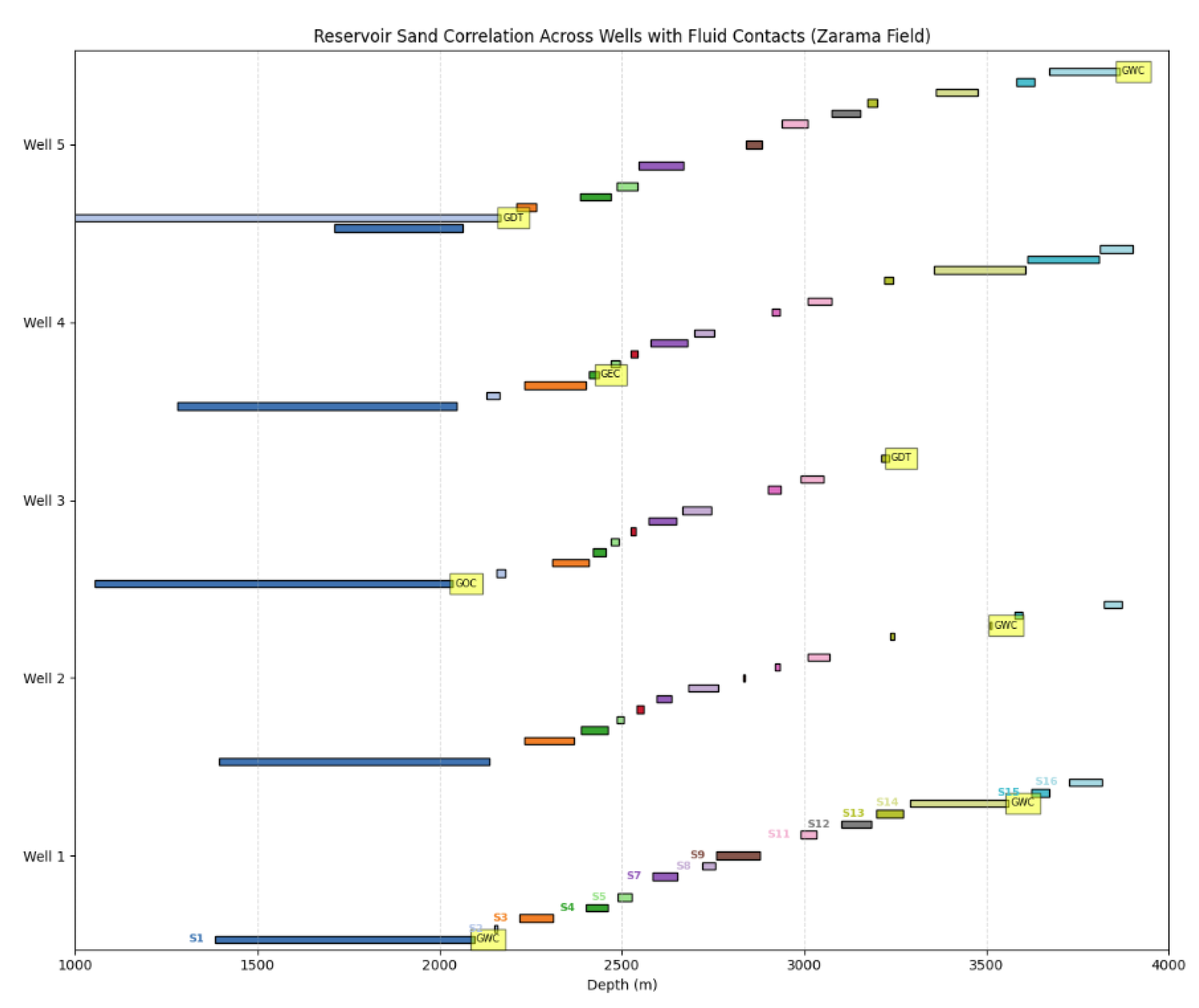
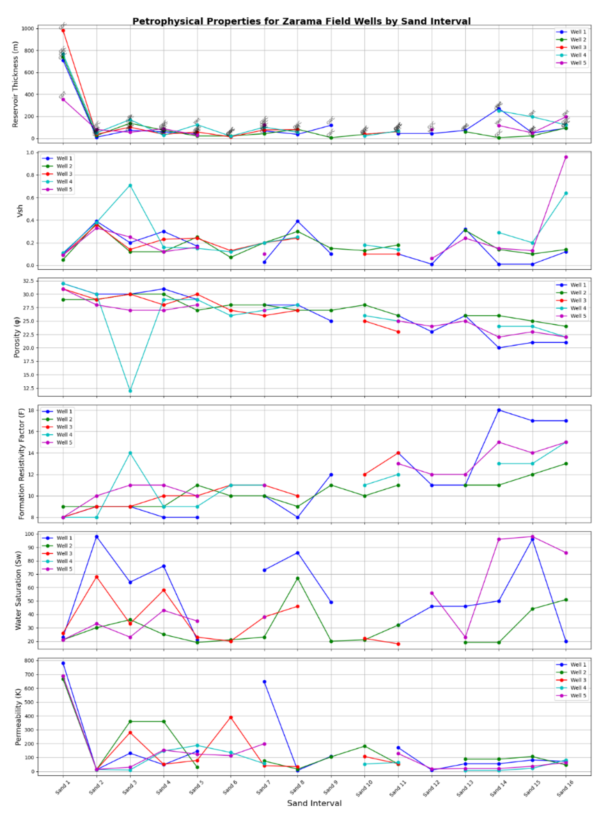
The field consists predominantly of numerous thin sand beds, displaying irregular and warped extents across wells, with significant thickness variation between wells. Sixteen reservoirs (S1–S16) are identified, distributed unevenly: fifteen in Well-2, fourteen each in Wells 1 and 4, thirteen in Well-5, and twelve in Well-3. Hydrocarbon column limits are defined by contacts such as gas-water (GWC), gas-oil (GOC), oil-water (OWC), gas-down-to-shale (GDT), and oil-down-to-shale (ODT). Porosity ranges from about 20% in S14 (Well-1) and S13 (Well-3) to 32% in upper sections of Wells 1 and 4, generally decreasing with depth. Permeability varies widely, from as low as 7 mD in S8 (Well-1) and S14 (Well-4) to as high as 781 mD in S1 (Well-1), strongly influenced by shale volume (Vsh) rather than depth. Some reservoirs, such as S12, S14, S15, and S16, are absent (pinched-out) in specific wells due to changes in sediment supply or transport energy. Water saturation varies between 13% and 98%, with net-to-gross ratios ranging from 1.0 to 0.36, underscoring reservoir heterogeneity(Figure 9).

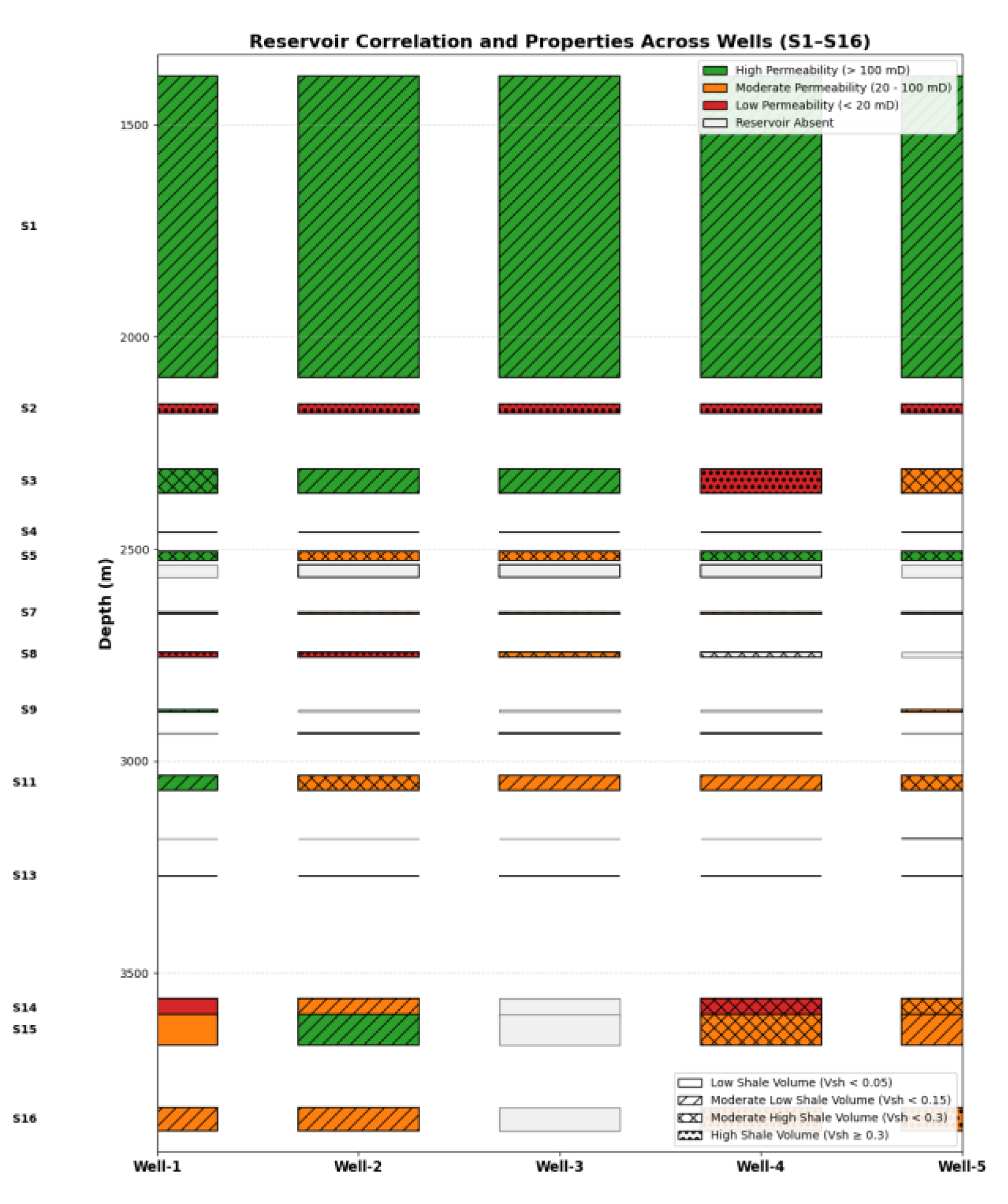
Reservoir thickness and net sand thickness positively influence hydrocarbon accumulation, while low shale volume (Vsh < 0.3) indicates good reservoir quality. Optimal porosity supports storage and flow, with water saturation (Sw) below 0.5 suggesting hydrocarbon presence. Permeability (K) enables hydrocarbon flow. Fluid contacts like GWC, GOC, GDT, and ODT mark hydrocarbon zones, whereas wet zones indicate water saturation or non-pay intervals. Hydrocarbon pore volume (HCPV) quantifies effective hydrocarbon volume. Sands with these markers and significant hydrocarbons are interpreted as pay zones. Thickness and fluid types assist in vertical and lateral reservoir delineation. For example, Sand 1 in Wells 1–5 shows large hydrocarbon volumes and contact markers, while zones labeled “Wet” typically signify non-pay intervals (Table 4).

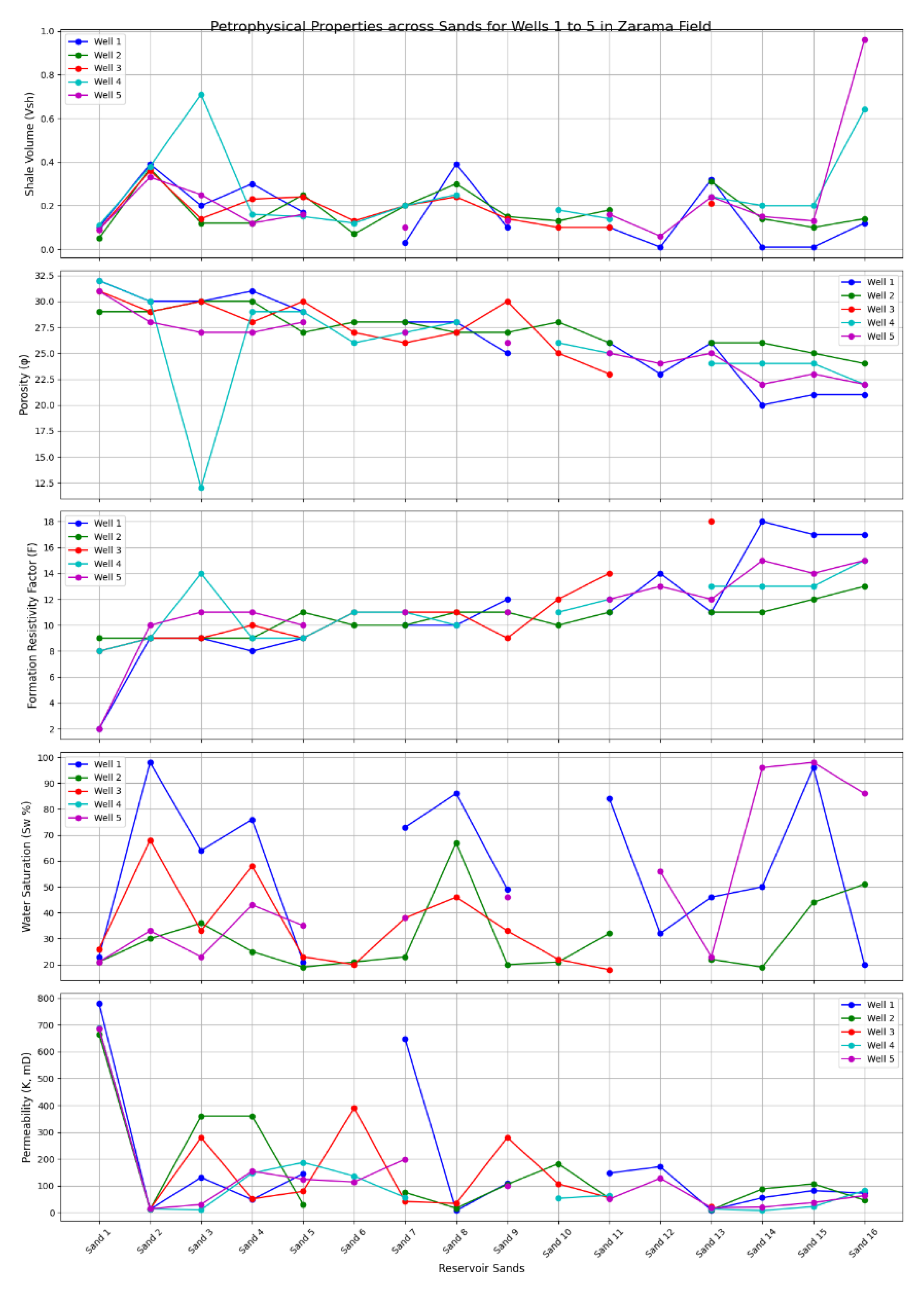
The thickness of the reservoir, as determined by detailed petrophysical analysis of sixteen sands in a number of wells, varies between thin beds (~6 m) and thick units (>700 m), with the volume of shale and porosity playing a dominant role in the quality of a reservoir. Zarama field consists mainly of gas-saturated sands having an oil/condensate gap both vertically and laterally. It should be noted that the thick laterally extensive sands, such as S1 and S3, are porous, highly permeable, and have large hydrocarbon pore volumes, which demonstrate their significance as reservoirs. The quality of thinner, shallower reservoirs that are more water-saturated is low. Shale-bearing strata have the effect of a fluid trap or barrier, thus affecting the distribution of hydrocarbons. The variations in the heterogeneous petrophysical properties depict typical Niger Delta deltaic variability that necessitates multi-well comprehensive evaluation in order to ensure proper reservoir characterization and development. In general, the data suggest that the reservoir system is gas-bearing with good production potential, which is moderated by variations in lithology and fluid distribution (Figure 10).

Table 5 presents a detailed petrophysical evaluation of five wells in the Zarama field, characterized by alternating sands and shales typical of the Agbada Formation, with reservoir thicknesses ranging from thin to very thick units. Shale volume (Vsh) varies significantly both within and between reservoirs, greatly affecting permeability more than porosity, which generally ranges between 20% and 32%. Permeability spans a wide range from 7 mD to 781 mD and is strongly influenced by shale content. Formation resistivity factors and water saturation data reveal fluid contacts such as gas-water, gas-oil, and oil-water. Key reservoir sands like S1 and S3 demonstrate high porosity, good permeability, and substantial hydrocarbon pore volume, indicating excellent production potential dominated by gas and some oil/condensate. Despite some log data gaps and gas-related density anomalies, integrated multi-well log analysis highlights vertical fluid presence and lateral heterogeneity, supported by shale seals. This assessment estimates recoverable hydrocarbons in millions of barrels of oil equivalent and large gas volumes, underscoring the importance of precise reservoir characterization for effective development planning.

Table 6 summarizes the depths of the identified reservoir sand units (S1 to S16) in six identified wells within the Zarama field. The majority of sand units (S1 to S5 and S7 to S11) exhibit good lateral continuity and are always similar across wells, with the depth of intervals juxtaposed closely across wells. Nevertheless, a few sands, e.g., S6, S8, S9, S12, S14, S15, and S16, are either missing or non-existent in a few wells, which means that there are vertical and lateral changes in the presence of the reservoirs, most probably because of the depositional heterogeneity or the truncation by erosion. The depth ranges also give minor differences between the wells, but are generally in the same trend in the Offshore Niger delta depositional Agbada Formation trend. This trend of correlation notes that although the reservoir sands tend to be more or less continuous vertically across the field, there are regions of local sand thinning, pinch-outs, or facies evolution that are of significance to get the reservoir mapped correctly and in planning the production (Figure 11).

Figure 11. Correlation of Reservoirs across the Wells in the Study Area.

Discussion and Conclusion

The reservoir of the study area, as shown by Wells 1-5, is of very good quality with the porosity value extending as high as 32 percent but generally hovering higher than 20 percent. Porosity is usually found to decrease with depth, which is probably due to the compaction effect that is stronger at depth in offshore environments. Results have shown that though porosity has a similar average at any well, permeability has great variations due to conflicting geology and reservoir variability. Well log analysis shows the possibility of compaction having begun earlier in older reservoirs, as there was a significant reduction of porosity in Wells 3 and 5 compared to Well 1. There is a moderate lateral consistency in the geologic and petrophysical properties, especially permeability, across the wells. Notably, though, there is quite a wide range of permeability very high ranging as high as 781 mD in Sand 1 (S1) of Well-1 to as low as 12 mD in Sand 2 (S2). Porosity is not the sole reason behind this variability, as the volume of shale (Vsh), or shale content, is also a key factor. The presence of a great volume of shale has a strong negative influence on permeability, and porosity acts as a positive influence, as it is expected that the presence of shale tends to destroy reservoir quality. The volumes of Shale in eastern wells (Wells 1 and 2) are larger than compared in the western wells (Wells 4 and 5), which shows that the sand development increases as one moves towards Well 5 (Figure 12).

Figure 12. Well-to-Well Reservoir Correlation in the Study area.

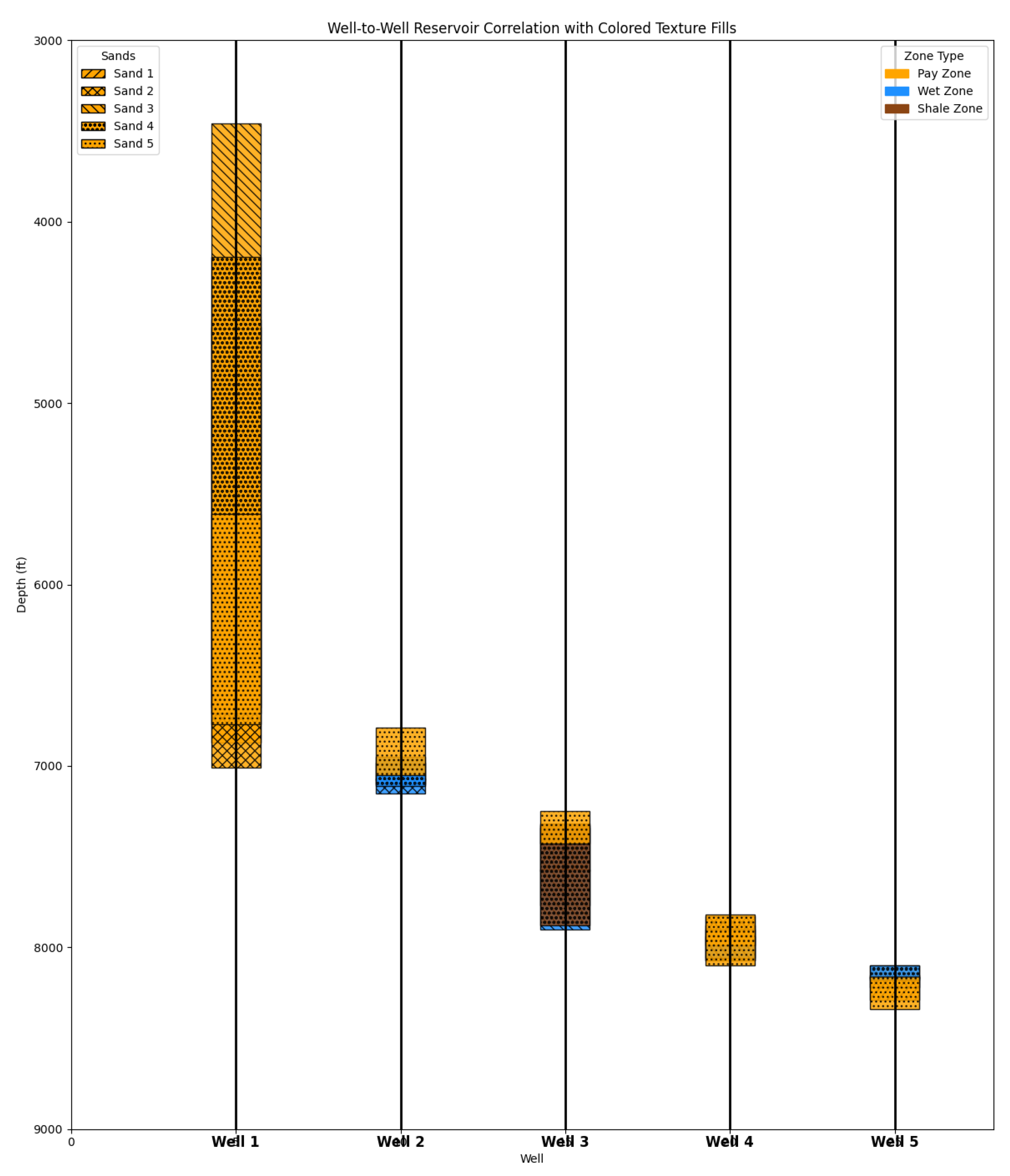
Petrophysical analysis shows that porosity, permeability, and thickness exhibit minor lateral variations, with reservoir thicknesses ranging from about 6 meters to over 700 meters. Unlike other Niger Delta reports, thickness does not increase with depth; instead, shale volume increases downward. Sands S1, S3, S14, and S16 are massive and likely continuous with good structural and stratigraphic traps in deeper offshore areas. Despite lacking core samples, wireline log-derived SE petrophysical parameters strongly correlate with nearby core data, yielding accurate estimates of water saturation (Sw) and cementation factors, supported by cross-plot RMS errors around 0.05. The Well-to-Well reservoir correlation visually replicates the similarities in sand zones across wells, providing a user-friendly representation of reservoir cross-sections and depth relationships. It uses color-coded zones (pay, wet, shale) and varied textures for sands to quickly identify lateral correlations and assess whether reservoir sands are continuous or heterogeneous in geometry. Well labels and depth scales allow clear visualization of stratigraphy, fluid trends, contacts, and potential pay zones. This correlation plot is crucial for reservoir characterization, enabling geoscientists and engineers to evaluate reservoir connectivity, continuity, and geological framework, aiding in volume estimation, development planning, and enhanced recovery decisions. Different textures improve strata distinction in complex stratigraphy, enhancing reservoir management through integrated geological and petrophysical data across multiple wells (Figure 13).

Figure 13. Well-to-Well Reservoir Correlation of the study Area.

The sand and shale regime makes an alternating sequence that was characteristic of the Agbada Formation, and it depicts sixteen reservoir sands with fluctuating thicknesses and lateral discontinuities. Other main parameters of the reservoirs that were calculated by using the known empirical models and log interpretation principles included shale volume, porosity, permeability, and fluid saturations. The porosity ranged between 20 to 32 % and in most cases exhibited a decreasing trend with depth, whereas permeability varied significantly between 7 mD and 781 mD, with the major factor affecting this being the content of shale. High resistivity and typical density-neutron log crossovers were used as an indication of gas-bearing zones, whereas oil and water zones were identified based on log responses and fluid saturation. Gas-water, gas-oil, and oil-water contacts were detected, and these helped in mapping hydrocarbon columns. The findings indicate that the Zarama field is heavily saturated with gas with oil/condensate fields, which are backed up by thick, wide sand sands, which are topped with thick, laterally continuous shale caps. Although there were difficulties to address such as poor quality of logs (density log anomalies caused by gas effects) and a few missing data gaps, the integrated log method was successful to give and characterized good estimates of hydrocarbon pore volumes and recoverable reserves say around 2.85 million barrels of oil equivalent and close to 5.85 billion cubic feet of gas. The existence of well variations in reservoir thickness and property is an indication of the lateral heterogeneity that is typical in the Niger Delta. The paper concludes that, in general, the research supports the good reservoir quality and high reserves potential and has a good petrophysical base to establish future development and production strategies of the Zarama field (Figure 13).

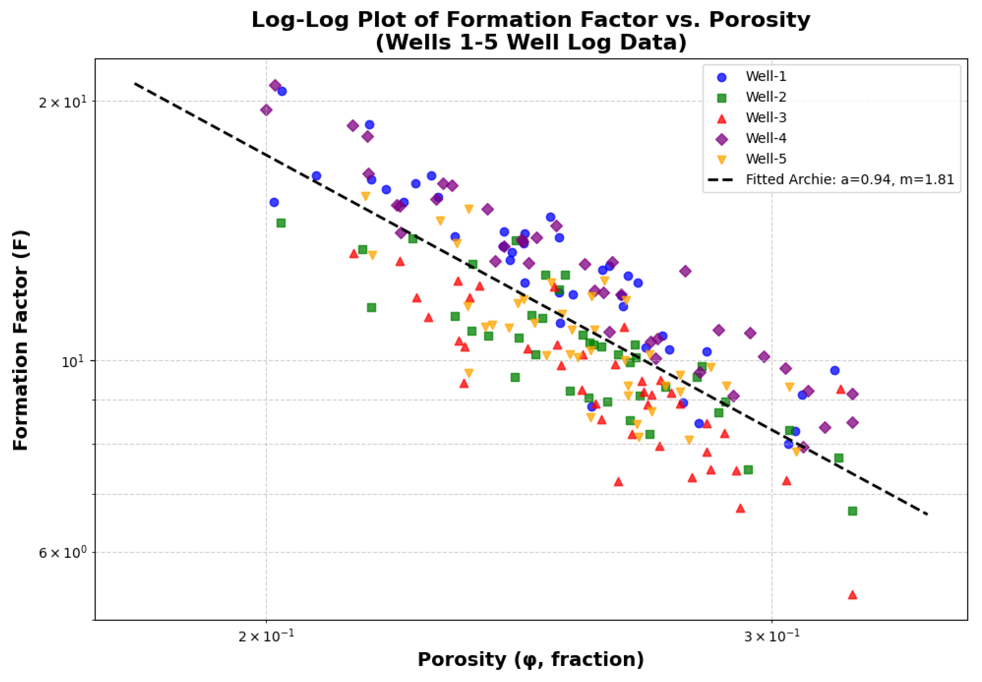
Figure 13. Log-log plot of Formation Factor as a function of Porosity for the Wells applying the equation log(F) = Log (a) – mlog (φ)derived from Archie’s Formation factor equation F=Ɵ^-m to the study area.

The study area predominantly features gas-bearing reservoirs, as indicated by high resistivity values—especially in the thick Sand 1 (S1)—and neutron log cross-overs observed in Wells 4 and 5. Notably, even at depths near 3872 m (S16, Well-2), porosity remains high, reaching up to 24%. Some oil-charged sands, mainly condensates, appear intermittently, such as at 2900 m depth in Well-3. Hydrocarbon accumulation is likely linked to pre-charge events during basin subsidence and structural deformation. Petrophysical indicators, including shale volume, porosity, permeability, and gamma ray logs, suggest generally homogeneous pay zones, mostly composed of thinly bedded sands consistent with Niger Delta patterns, where over 70% of oil columns are under 15 m thick. Resistivity variations reflect changes in porosity, clay content, and hydrogen index, with resistivity anomalies due to clay-bound water. Hydrocarbon column thickness varies widely—Well-2’s is about 6 m, whereas Well-3 may exceed 830 m, unusually thick for the Niger Delta. Thick reservoirs like S1 show gas accumulation suggested by resistivity and density logs, although confirming seals above is limited by data gaps. Core S13’s gas-filled zones, capped by ~165 m shale, exemplify lateral structural trapping. (Figure 12).

Hydrocarbon zones mainly occur within these depth ranges in the wells (Table 4):

Well 1: 1384–2095 m, 1396–2137 m, 1055–2037 m, 1279–2046 m, 1710–2064 m (all marked with GWC, GOC, GDT, GEC indicating hydrocarbon presence)

Well 2: The pay zone near 2070–2149 m (GWC), while upper intervals (2149–2159 m to 2119–2168 m) are wet zones.

Well 3: Mixed wet and shale zones, but pay zones around 2210–2265 m (GWC) and similar intervals.

Well 4: Hydrocarbon zones around 2387–2460 m, 2409–2436 m, 2384–2470 m with GWC, while some intervals are wet.

Well 5: Pay zones roughly 2488–2543 m, with GOC and ODT markings, generally hydrocarbon bearing.

The general findings on the reservoir quality, the variability, the petrophysical controls, reservoir architecture, the presence of hydrocarbons, and the implications of production in the study area Wells 1-5.

Conclusion

Characteristic description of the reservoir property of the study region consists of Wells 1 to 5, a very good quality reservoir with porosity level in the range of high up to 32 percent, with the overall average above 20 percent, showing a general pattern to decrease with depth, probably because of compactation effects in that offshore location. Although average porosity between wells is similar, permeability exhibits strong lateral and vertical gradients-ranging between very high (781 mD in Sand 1 of Well 1) to very low values-and it is largely influenced by the extent of shale volume, which is detrimental to permeability and reservoir quality. The structural and stratigraphic trapping of heterogeneous but predominantly gas-bearing reservoir sands is confirmed by petrophysical analysis, which is also supported by the lateral continuity in the level of well-to-well correlation, which visually represents correlated pay, wet and shale zones, aiding in defining the architecture of the reservoir and distribution of the fluids. Zone bearing hydrocarbons are mainly located in the ranges of depth between 1055m and 2543m across wells, which is strengthened by the use of the cross-plot analysis and fluid saturational factors highlighting contact points that are the GWC, GOC, and GDT. The reservoir contains a combination of thick and thin layers of sand with wide ranges of shale and loads of fluids that represent gas plus some oil condensates. The combined petrophysical statistics determine a non-homogeneous yet gas-bearing reservoir complex with a great prospect of production achievement. Deviation of petrophysical properties between wells supports the need for multi-well combined methodologies of evaluation to provide an optimal strategy in considering reservoir characterization and development mechanisms. Although petrophysical heterogeneity requires integrated multi-well assessment, the result indicates a high hydrocarbon prospect with a recovery volume as near as 2.85 million barrels of oil equivalent, and almost 5.85 billion cubic feet of gas. This multifaceted study in the background of strategic reservoir management and development planning provides the best production optimization of the offshore reservoir with a complex, highly structural, and stratigraphic setting.

References

Ahmad Afshar, Maysam Abedi, Gholam-Hossain Norouzi, Mohammad-Ali Riahi. (2015): Geophysical investigation of underground water content zones using electrical resistivity tomography and ground penetrating radar: A case study in Hesarak-Karaj, Iran. Engineering Geology. Volume 196, 28 September 2015, Pages 183-193.
Bension Sh. Singer and Kurt-M. Strackz. (1998): New aspects of through-casing resistivity theory. GEOPHYSICS, VOL. 63, NO. 1 (JANUARY-FEBRUARY 1998); P. 52–63, 8 FIGS.
Darwin V. Ellis Julian M. Singer. (2008): Well Logging for Earth Scientists Second Edition. Library of Congress Control Number: 2008921855. ISBN 978-1-4020-3738-2 (HB). ISBN 978-1-4020-4602-5 (e-book). Published by Springer, www.springer.com Printed on acid-free paper ISBN 978-1-4020-4602-5 (e-book). Pp 1-692.
DEPARTMENT OF THE ARMY EM 1110-2-1420 U.S. Army Corps of Engineers CECW-CE Washington, DC 20314-1000 (2018). Engineering and Design HYDROLOGIC ENGINEERING REQUIREMENTS FOR RESERVOIRS.
Derek Eamus, Ray Froend, Robyn Loomes, Grant C. Hose, and Brad Murray. (2006): A functional methodology for determining the groundwater regime needed to maintain the health of groundwater-dependent vegetation.Australian Journal of Botany 54(2):97-114. [CrossRef]
EMOYAN, O. O., AKPOBORIE I. A. and AKPORHONOR E. E. (2008): The Oil and Gas Industry and the Niger Delta: Implications for the Environment. J. Appl. Sci. Environ. Manage. September, 2008 Vol. 12(3) 29 – 37.
Geoffrey Page and Stephen Vickers. “The Petrophysics of Drilling Fluids and Their Effects on Log Data.” Petrophysics 52 (2011): 369–380.
Hina Ahmed and Manahil Sameer. (2024): Geological Analysis and Subsurface Characterization Through Well-Log Analysis: Insights into Reservoir Evaluation and Petrophysical Properties https://www.researchgate.net/publication/384920379. [CrossRef]
Mehdi Saffari, and Pooria Kianoush (2025): Integrated petrophysical evaluation of Sarvak, Gadvan, and Fahliyan formations in the Zagros Area: insights into reservoir characterization and hydrocarbon potential Journal of Petroleum Exploration and Production Technology (2025) 15:54. [CrossRef]
Naiem Souilam Sobih, Ahmed Ahmed El Nagar, Ali Elsayed Abbas1 and Samir Shehab (2025): Integrating petrophysical characterization and reservoir evaluation of the Kafr ELSheikh formation in Sapphire field, Nile Delta, Egypt. Scientific Reports | (2025) 15:4555 |. [CrossRef]

Figure 2. Densities of common lithologies (After, 1989).

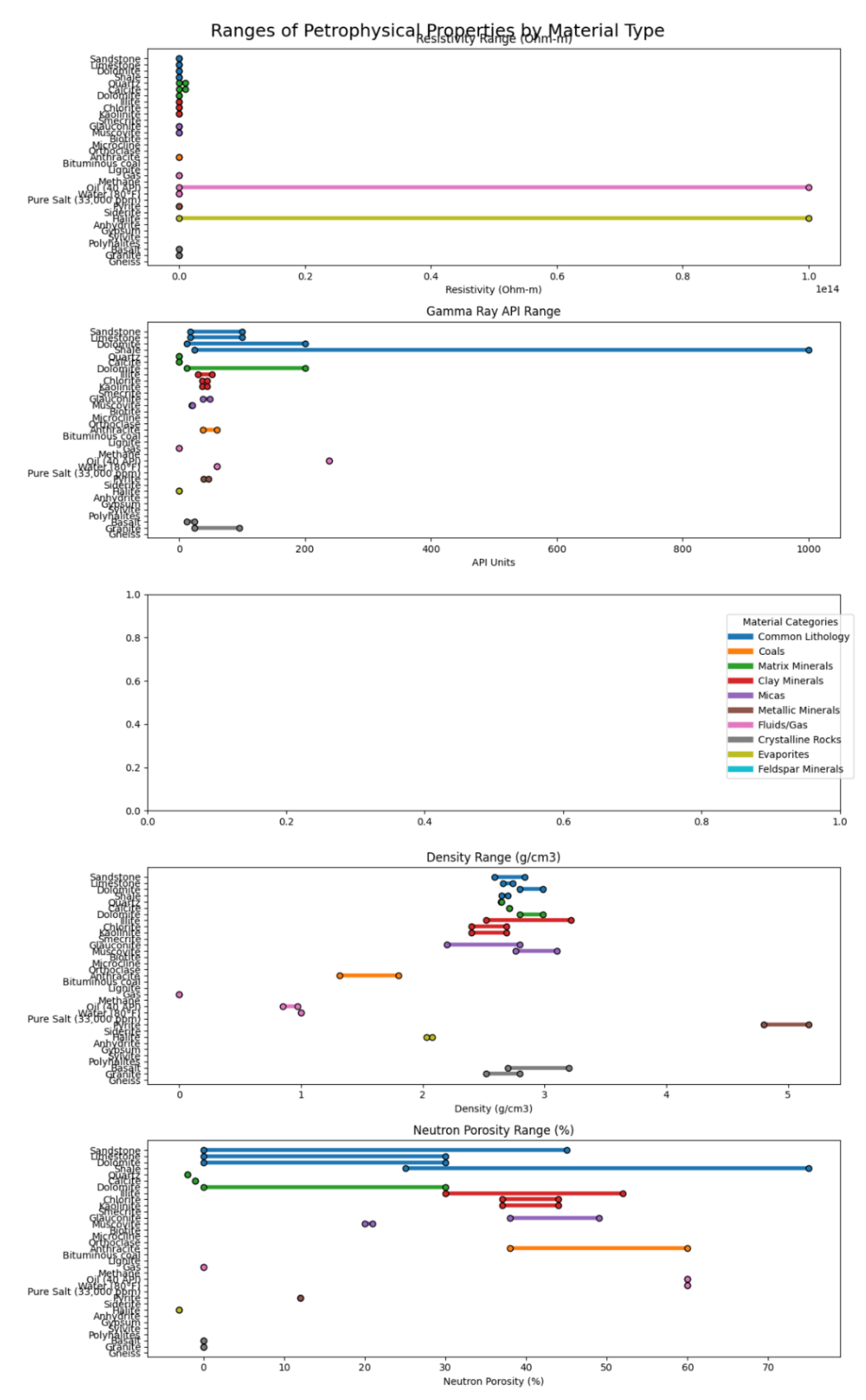
Figure 3. Resistivity, Gamma Ray, Transit time, Density, and Neutron value of different materials.

Figure 4. Resistivity and Density logs of Well 1.

Figure 5. Gamma Ray, Resistivity, and Density logs of Well 2.

Figure 6. Gamma Ray Resistivity and Density logs of Well 3.

Figure 7. Gamma Ray and Neutron logs of Well 4.

Figure 8. Resistivity, Neutron, Porosity, and Average Logs.

Figure 9. Results of Petrophysical Analysis of Sands S1 to S16 of the study Area.

Figure 10. Comparison of Petrophysical Analysis in the study area.

Table 1. The Z/A ratios for sandstone, limestone, and dolomite are:.

Rock type		Z/A Ratio
Sandstone: (SiO2)		Z/A=0.499
Limestone: (CaCO3)		Z/A=0.500
Dolomite: (CaMg(CO3)2)		Z/A-0.499

Table 2. Densities of common lithologies (from Schlumberger, 1989).

Lithology	Range (g/cm³)	Matrix (g/cm³)
Clay-shales	1.8 - 2.75	Varies (Ave. 2.65-2.7)
Sandstone	1.9 – 2.65	2.65
Limestone	2.2 – 2.71	2.71
Dolomites	2.3 – 2.87	2.87

Table 3. Resistivity, Gamma Ray, Transit time, Density, and Neutron value of different materials. Adopted after Schlumberger 1989.

	Material	Resistivity (Ohm-m)	Gamma Ray API API^(o)	Δtma	Density (g/cm³) (ma)	Neutron porosity
Common lithology	Sandstone Limestone Dolomite Shale	Top 1000 80-6 X 10³ 1-7 X 10³ 0.5 - 1000	18 – 160 18 – 100 12 - 200 24 - 1000	53 - 1000	2.59 -2.84	0 – 45
				47.6 - 53	2.66 – 2.74	0 – 30
				38.5 – 45	2.8 -2.99	00 -3-
				60 -170	2.65 – 2.7	25 - 75
Matrix minerals	Quartz Calcite Dolomite	10⁴ - 10¹² 10² - 10¹² 1-7 X 10³	000	51.2 – 56.0	2.64 – 2.65	-2
				45.5 -49.0	2.71	-1
				38.5 – 45.0	2.85 -2.88	1
Clay minerals	Illite Chlorite Kaolinite Smecrite	------- ------- ------- -------	250 - 300 180 – 250 50 – 130 150 -200	-----	2.52 – 3.00	30
				-----	2.60 -3.22	52
				-----	2.40 – 2.69	37
				-----	2.00 – 3.00	44
Micas	Glauconite Muscovite Biotite		75 - 90	-----	2.2 – 2.8	38
		10^-11 - 10¹²	140 -270	49	2.76 -3.1	20
		10¹⁸ - 10²³	90 -275	50.8 – 51	2.65 – 3.1	21
Feldspar Minerals	Microcline Orthoclase	-----	220 -280	45	2.53 – 2.57	30
Feldspar Minerals	Microcline Orthoclase	-----	220 - 280	69	2.52 -2.63	30
Coals	Anthracite Bituminous coal Lignite	10^-9 - 10²³	0	90 - 120	1.32 – 1.80	38
		10 - 10²	0 – 18	100 - 140	1.15 – 1.7	60
		4 - 10³	6 - 24	140 -180	0.5 – 1.5	52
Fluids/Gas	Gas Methane Oil (40⁴) API Pure water Salt water (33,00ppm)	ά	0	-----	0.000386	-----
		ά	0	626	0.00076	-----
		10⁷ - 10¹⁴	0.12 – 0.40	238	0.85 – 0.97	60
		ά	0	189 - 207	1.00	100
		0.031	0	180	1.19	60
Metallic Minerals	Pyrite Siderite	10-⁴ - 10^-2	-----	39.2 -39	4.8 – 5.17	-3
Metallic Minerals	Pyrite Siderite	10² - 1000	0	47	3.0 – 3.89	12
Evaporites	Halite Anhydrite Gypsum Sylvite Polyhalites	<10² - 101⁴	0	66.7 - 67	2.03 – 2.08	-3
		10² - 10¹⁴	0 – 12	50	2.89 – 3.05	-2
		1000	0	52 - 53	2.33 – 2.40	60
		10²⁰ - 10²⁴	500	74	1.86 – 1.99	-3
		-----	200	57.5 - 58	2.79	25
Crystalline rocks	Basalt Granite Gneiss	6 x 10² - 10⁴	12 - 24	45 – 57.5	2.7 – 3.2	-----
		10⁶	24 - 96	46.8 – 53.5	2.52 – 2.8	-----
		10² - 10⁶	24 - 48	48.8 – 51.6	2.6 -3.04	-----

Table 4. Results of Petrophysical Analysis of Sands S1 to S16 of the study Area.

Sand	Well	Sand interval	Sand interval	Reservoir thickness		V_sh	φ	F	S_w	K	Fluid	Remark	HCPV
1	1	4540-6870	1384-2095	711	698	0.10	32	8	23	781	1796	GWC	663824.7 barrel of oil + 1312227 Scf of gas
	2	4580-7010	1396-2137	741	670	0.05	29	9	21	666	1915	GDT
	3	3460-6680	1055-2037	982	830	0.09	31	8	26	687	1723	GOC
	4	4195-6710	1279-2046	767	665	0.11	32	8		688	1954	GEC
	5	5610-6770	1710-2064	354	311	0.09	31	8	21	687	2061	GDT
2	1	7050-7080	2149-2159	10	10	0.39	30	9	98	12	Wet	Wet	499149 Scf of gas
	2	7070-7150	2155-2180	25	22	0.37	29	9	30	12	Wet	Wet
	3	6980-7100	2128-2165	37	33	0.36	29	9	68	13	Wet	Wet
	4	6950-7110	2119-2168	49	39	0.38	30	9		13	Wet	Wet
	5	6790-7050	2070-2149	79	60	0.33	28	10	33	14	2085	GWC
3	1	7340-7580	2238-2311	73	53	0.20	30	9	64	131	Wet	Sh	106293.6 Scf of gas
	2	7329-7770	2232-2369	137	89	0.12	30	9	36	360	Wet	GWC
	3	7570-7900	2308-2409	101	76	0.14	30	9	33	280	2348	Wet
	4	7320-7880	2232-2402	170	51	0.71	12	14		10	Sh	GWC
	5	7250-7430	2210-2265	55	41	0.25	27	11	23	30	2244	GWC
4	1	7880-8070	2402-2460	58	46	0.30	31	8	76	48	Wet	Wet	612521.8.9 Scf of gas
	2	7830-8070	2387-2460	73	61	0.12	30	9	25	360	2430	GWC
	3	7940-8060	2421-2457	36	32	0.23	28	10	58	51	Wet	Wet
	4	7900-7990	2409-2436	27	12	0.16	29	9		147	2427	GWC
	5	7820-8100	2384-2470	86	49	0.12	27	11	43	154	2463	GWC
5	1	8160-8290	2488-2527	39	29	0.17	29	9	21	145	2500	GOC	1889930 barrel of oil + 4187172 Scf of gas
	2	8150-8220	2485-2506	21	29	0.25	27	11	19	30	2500	ODT
	3	8100-8170	2470-2492	21	16	0.24	30	9	23	79	2488	ODT
	4	8100-8180	2470-2494	24	21	0.15	29	9		187	Wet	Wet
	5	8160-8340	2486-2543	57	50	0.16	28	10	35	124	2521	GWC
6	1	---------	-------	------	------	------	----	----	----	----	-----	------	37490 Scf of gas
	2	8330-8400	2540-2561	21	21	0.07	28	10	21	390	2555	GWC
	3	8280-8320	2524-2537	13	11	0.13	27	11	20	136	2534	GWC
	4	8280-8340	2524-2543	19	19	0.12	26	11		114	2537	GWC
	5	----------	-----------	-----	-----	-----	-----	-----	----	-----	-----	-----
7	1	8480-8700	2585-2652	67	58	0.03	28	10	73	647	Wet	Wet	124846.3 of Scf gas
	2	8510-8650	2595-2637	42	38	0.20	28	10	23	75	2607	GWC
	3	8440-9690	2573-2649	76	40	0.20	26	11	38	41	2622	GWC
	4	8460-8790	2579-2680	101	45	0.20	27	11		56	2619	GWC
	5	8350-8750	2546-2668	122	72	0.10	27	11	38	199	2640	GWC
8	1	8920-9040	2720-2756	36	30	0.39	28	10	86	7	Sh	Sh	166377.8 barrel of oil + 59598 Scf of gas
	2	8800-9070	2683-2765	82	36	0.30	27	11	67	16	Sh	Sh
	3	8740-9000	2665-2744	79	38	0.24	27	11	46	34	2732	OWC
	4	8850-9030	2698-2753	55	20	0.25	28	10	40	----	WET	Wet
	5	--------	--------	----	------	-----	-----	-----	----	----	-----	------
9	1	9050-9440	2759-2878	119	90	0.10	25	12	49	109	2854	GWC	18802.7 barrel of oil+74114 Scf of gas
	2	9290-9310	2832-2838	6	6	0.15	27	11	20	105	2927	GDT
	3	9579-7900	2308-2409	101	76	0.14	30	9	33	280	2348	GWC
	4	-------	-------	------	-----	-----	-----	-----	----	-----	-----	-----
	5	9320-9460	2841-2884	43	36	0.13	26	11	46	100	2866	GOC
10	1	-------	---------	----	-----	-----	-----	-----	----	------	------	------	90135.4 barrel for oil + 44452.3 Scf of gas
	2	9570-9690	2918-2954	36	33	0.13	28	10	21	182	2939	GWC
	3	9510-9630	2899-2936	37	34	0.10	25	12	22	107	2933	ODT
	4	9550-9620	2912-2933	21	20	0.18	26	11		53	2927	GWC
	5	-------	--------	------	-----	-----	-----	-----	----	-----	------	-----
11	1	9810-9950	2991-3034	43	37	0.10	26	11	84	147	Wet	Wet	108232.3 Scf of gas
	2	9870-10070	3009-3024	61	40	0.18	26	11	32	53	3061	GWC
	3	9810-10010	2991-3052	61	39	0.10	23	14	18	55	3049	GDT
	4	9870-10090	3009-3076	67	55	0.16	25	12		64	3076	GWC
	5	9640-9870	2939-3009	70	43		25	12		50	Wet	Wet
12	1	10170-10440	3101-3183	82	74	0.01	23	14	32	171	3159	GOC	17631.8 barrel of oil + 65939.5 Scf of gas
	2	--------	-------	------	------	------	-----	------	----	------	------	------
	3	--------	-------	------	------	------	-----	------	----	------	------	------
	4	--------	-------	------	------	------	-----	-------	----	------	------	------
	5	10090-10350	3076-3155	79	38	0.06	24	13	56	128	3116	GOC
13	1	10490-10350	3198-3271	72	60	0.32	26	11	46		3259	GDT	59685.7 Scf of gas
	2	10610-10650	3235-3247	12	12	0.31	26	11	22	10	3244	GDT
	3	10530-10600	3210-3232	22	13	0.21	20	18	18	23	3231	GDT
	4	10560-10640	3220-3244	24	17	0.24	24	13		13	3241	GDT
	5	10410-10530	3174-3210	36	20	0.24	25	12	23	18	3201	GDT
14	1	10790-11680	3290-3561	271	215	0.01	20	18	80	55		Wet	313611.9 Scf of gas
	2	11510-11530	3509-3515	6	6	0.14	26	11	19	88	3515	GOC
	3	--------	--------	------	------	------	-----	------	----	------	------	-------
	4	11010-11830	3357-3607	250	240	0.29	24	13		7	3598	GWC
	5	11020-11400	3360-3476	116	89	0.15	22	14	96	20	Wet	Wet
15	1	11880-12040	3622-3671	49	40	0.01	21	17	96	82	Wet	Wet	5345.45 barrel of oil + 19600 Scf of gas
	2	11730-11800	3576-3598	22	10	0.10	25	12	44	107	3588	GOC
	3	--------	--------	-----	-----	-----	-----	------	----	------	------	------
	4	11850-12490	3613-3808	195	190	0.20	24	13		22	Wet	Wet
	5	11750-11910	3582-3631	49	38	0.13	23	14	98	37	Wet	Wet
16	1	12220-12520	3726-3817	91	86	0.02	21	17	20	72	3802	GWC	114849.7 Scf of gas
	2	12540-12700	3823-3872	94	30	0.14	24	13	51	46	3860	GWC
	3	-------	------	-----	-----	------	-----	-----	----	----	-----	------
	4	12500-12900	3811-3933	122	118	0.04	22	15	----	82	3887	GWC
	5	12040-12680	3671-1866	195	103	0.06	22	15	86	63	Wet	Wet

Table 5. Comparison of Petrophysical Analysis in the study area.

PROPERTY	Well	Sand
		1	2	3	4	5	6	7	8	9	10	11	12	13	14	15	16
V_sh	1	0.10	0.39	0.20	0.30	0.17	-----	0.03	0.39	0.10	-----	0.10	0.01	0.32	0.01	0.01	0.12
	2	0.05	0.37	0.12	0.12	0.25	0.07	0.20	0.30	0.15	0.13	0.18	----	0.31	0.14	0.10	0.14
	3	0.09	0.36	0.14	0.23	0.24	0.13	0.20	0.24	0.14	0.10	0.10	----	0.21	----	----	----
	4	0.11	0.38	0.71	0.16	0.15	0.12	0.20	0.25	-----	0.18	0.14	----	0.24	0.20	0.20	0.64
	5	0.09	0.33	0.25	0.12	0.16	----	0.10	----	0.13	----	0.16	0.06	0.24	0.15	0.13	0.96
Porosity (φ)	1	32	30	30	31	29	----	28	28	25	-----	26	23	26	20	21	21
	2	29	29	30	30	27	28	28	27	27	28	26	----	26	26	25	24
	3	31	29	30	28	30	27	26	27	30	25	23	----	-----	-----	----	----
	4	32	30	12	29	29	26	27	28	-----	26	25	----	24	24	24	22
	5	31	28	27	27	28	----	27	----	26	----	25	24	25	22	23	22
F	1	2	9	9	8	9	----	10	10	12	----	11	14	11	18	17	17
	2	9	9	9	9	11	10	10	11	11	10	11	----	11	11	12	13
	3	8	9	9	10	9	11	11	11	9	12	14	----	18	----	----	-----
	4	8	9	14	9	9	11	11	10	-----	11	12	----	13	13	13	15
	5	2	10	11	11	10	-----	11	----	11	-----	12	13	12	15	14	15
S_w	1	23	98	64	76	21	-----	73	86	49	-----	84	32	46	50	96	20
	2	21	30	36	25	19	21	23	67	20	21	32	----	22	19	44	51
	3	26	68	33	58	23	20	38	46	33	22	18	-----	-----	-----	-----	----
	4	-----	-----	----	----	----	----	-----	40	-----	-----	-----	-----	-----	-----	-----	-----
	5	21	33	23	43	35	-----	38	-----	46	-----	-----	56	23	96	98	86
K(mD)	1	781	12	131	48	145	-----	647	7	109	-----	147	171	9	55	82	72
	2	666	12	360	360	30	-----	75	16	105	182	53	-----	10	88	107	46
	3	687	13	280	51	79	390	41	34	280	107	55	-----	23	-----	-----	-----
	4	688	13	10	147	187	136	56	-----	-----	53	64	-----	13	7	22	82
	5	687	14	30	154	124	114	199	-----	100	----	50	128	18	20	37	63

Table 6. Correlation of Reservoirs across the Wells in the Study Area.

	Well 1	Well 2	Well 3	Well4	Well 5
	Reservoir interval (m)
S₁	1384-2095	1396-2137	1055-2037	1279-2046	1710-2064
S₂	2149-2159	2155-2180	2128-2165	219-2168	2070-2149
S₃	2218-2311	2232-2369	2308-2409	2232-2402	2210-2265
S₄	2402-2460	2387-2460	2421-2457	2409-2436	2384-2470
S₅	2488-2527	2485-2506	2470-2491	2470-2494	2486-2543
S₆	---------	2540-256	2524-2537	2524-2543	---------
S₇	2585-2652	2595-2637	2573-2649	2579-2680	2546-2668
S₈	2720-2756	2683-2765	2665-2744	2698-2753	-------
S₉	2759-2878	2832-2838	-------	--------	2841-2884
S₁₀		2918-2934	2899-2936	2912-2933	---------
S₁₁	2991-3034	3009-3070	2991-3052	3009-3076	2939-3009
S₁₂	3101-3183	-------	--------	--------	3076-3155
S₁₃	3198-3271	3235-3247	3210-3232	3220-3244	3174-32)0
S₁₄	32.90-3561	3509-3S15	------	3357-3607	3360-3476
S₁₅	3622-3671	3576-3598	--------	3613-3808	3582-3631
S₁₆	3726-3817	3823-3872	------	3811-3900	3671-3866

Disclaimer/Publisher’s Note: The statements, opinions and data contained in all publications are solely those of the individual author(s) and contributor(s) and not of MDPI and/or the editor(s). MDPI and/or the editor(s) disclaim responsibility for any injury to people or property resulting from any ideas, methods, instructions or products referred to in the content.

© 2025 by the authors. Licensee MDPI, Basel, Switzerland. This article is an open access article distributed under the terms and conditions of the Creative Commons Attribution (CC BY) license (http://creativecommons.org/licenses/by/4.0/).

Copyright: This open access article is published under a Creative Commons CC BY 4.0 license, which permit the free download, distribution, and reuse, provided that the author and preprint are cited in any reuse.

Integrated Petrophysical Evaluation and Reservoir Characterization of the Zarama Field, Offshore Niger Delta Using Multi-Well Geophysical Log Analysis

Abstract

Keywords:

Subject:

Introduction

Method and Materials

Data Analysis

Petrophysical Data Analysis

Fluid detection

Results

Discussion and Conclusion

Conclusion

References

MDPI Initiatives

Important Links

Subscribe