
Submitted:
01 July 2025
Posted:
03 July 2025
You are already at the latest version
Abstract
This study offers a comprehensive petrophysical evaluation and reservoir characterization of the Srikail Gas Field, situated on the Tripura Uplift in the east-central Bengal Basin. Utilizing well log data from four wells (Srikail-1 to Srikail-4), the analysis targets the Bhuban and Bokabil formations of the Surma Group. Standard log suites, including gamma ray, spontaneous potential, caliper, resistivity, neutron, density, and sonic logs, were interpreted using both manual techniques and digital analysis through Techlog software. Key petrophysical properties, including shale volume, effective porosity, fluid saturations, permeability, and bulk volume of water, were estimated using a combination of empirical modeling and automated interpretation workflows. Cross-plot methodologies were applied to assist in reservoir evaluation. The study integrated both qualitative and quantitative approaches to characterize each reservoir unit in detail.
Results demonstrate significant heterogeneities in reservoir quality across the field. While some intervals exhibit favorable properties suitable for commercial gas production, others are characterized by high carbonate content, poor porosity, and very low permeability, indicative of tight to semi-conventional reservoirs. The most productive zones, identified as the D sands, are cleaner sands with excellent permeability (102mD to 355mD). In contrast, deeper intervals generally exhibit tighter characteristics, with DST-derived permeability values ranging from 0.6 to 0.01 mD. The study recommends integrating core analysis and 3D seismic data with well log interpretation in future work to improve reservoir delineation and support more effective development strategies in the Srikail Gas Field.
Keywords:
petrophysics
; reservoir characterization
; shaly sands
; Bengal Basin
1. Introduction
Wireline logging data can provide valuable information for oil and gas exploration, such as reservoir characteristics, hydrocarbon potential, and formation evaluation. However, interpreting wireline logging data can be challenging, because economic and efficient oil and gas production is highly dependent on understanding key properties of reservoir rock, such as porosity, permeability, and wettability [1].
The determination of reservoir quality largely depends on quantitative and qualitative evaluation of petrophysical properties. Petrophysical parameters, i.e., Effective Porosity (Φeff), Effective Water Saturation (Sw), Formation Water Resistivity (Rw), Hydrocarbon Saturation (Shc-eff), and Permeability, all of them may be evaluated using well log data, thus performing a correct reservoir characterization.
This study addresses the formation evaluation and reservoir characterization of shaly sands at the Srikail Gas field (Bengal Basin), based on a detailed analysis of to all available mud log data and wire line log data. The analysis used the Symandox Method [2,3], with empirical mathematical equations appropriate for shaly sands. Numerous previous studies on the petrophysical analysis and reservoir characterization of Miocene sand [4,5,6,7,8] reservoirs across various gas fields within the Bengal Basin have contributed to the interpretation and analysis presented in this study.
2. Geological Framework
The study area lies in the east-central part of the Bengal Basin (Figure 1) [9,10]. The study was done in the Srikail gas field located about 60 km east of Dhaka city and approximately 100 km away from the Surma sub-basin.
The Bengal Basin formed during the continental extension of the eastern part of Gondwana, during the Late Mesozoic and is still ongoing [11]. During the Cenozoic, the Indian plate rifted northwest and then northwards from the combined Antarctica–Australia part of Gondwana, resulting in a major collision between India and Asia in the Miocene. As a result, the Himalayas in the north and the Indo-Burman range in the east were gradually uplifted as the Tethys Sea closed [12]. Tectonically, the Srikail anticline is located on the western part of the folded belt of Bengal Foredeep within the Tripura Uplift of the Bengal Basin (Figure 2) [13].
The existing stratigraphic system for the Bengal Basin was based exclusively on lithostratigraphic association with the type sections described by Evans [14] in Assam, northeastern India, along the fold belt in the basin's eastern portion. Evans' stratigraphic age estimates for the Assam sequences are questionable since they are based on long-distance correlations between brackish marine macrofauna and vertebrate findings. While some parts of Evans' scheme may be usable in the regional lithostratigraphic or seismic correlation (e.g., the boundary between the Surma and Tipam Groups), other parts of his classification (e.g., the contact between the Bhuban and Bokabil Formations or the internal units of these formations) are difficult to apply to the lithostratigraphic succession throughout the basin. For the Central Basin, which includes the Surma Basin and the Srikail Gas Field, the proposed lithostratigraphy is depicted in Figure 3 [13].
The focus of this study is the Miocene to Early Pliocene Surma Group, which does not outcrop in the study area. The Surma Group sediments were deposited in a large mud-rich prograding delta system, in response to the western encroachment of the Indo-Burma range and rising Himalaya, the [15]. Most authors have traditionally divided the Surma Group into two units based on Evan's stratigraphic scheme [14], with the younger Bokabil Formation covering the older Bhubhan Formation [16,17,18].
The Bhuban Formation has been interpreted by Johnson and Alam [19] as prodelta to delta front deposits of a mud-rich delta system, while te Bokabil sediments correspond to subaerial to brackish sandy deposits [16]. Sultana and Alam [20] interpreted the sediments of this group as shallow marine to tide-dominated coastal deposits within a transgressive - regressive regime based on extensive logging of core samples from the Sylhet Trough. The top of the Surma group is dominated by a shaley unit known as the "Upper Marine Shale" (UMS) [16].
The thickness of the Surma Group ranges from 2700 m to over 3900 m. Based on seismic data, mud logs, and wireline log responses, multiple prospective sand zones (named A to K,
3. Materials and Methods
3.1. Materials
This study involves the analysis of four wells (Figure 4), where distinct reservoir zones have been identified in each (Table 1 and Table 2).
Wireline log data have been analysed to calculate petrophysical parameters and characterize the reservoirs. Srikail wells have been covered by all suites of resistivity and porosity logs, along with GR and SP logs. The open hole composite logs which are used in this study were conducted in different stages are as follows (Table 3):
All the stages of logging were conducted by China Petroleum Logging Company Ltd. (CPL) and covered all sets of logs. Overall quality of logs was found to be satisfactory.
3.2. Methods
3.2.1. Petrophysical Workflow
Petrophysical analysis was conducted on all the identified reservoirs, based on mud log and wireline log data. The following methodological steps were undertaken:
- Geological and geophysical data were thoroughly reviewed.
- Wireline log data were compiled for both manual interpretation [23] and imported into petrophysical software (Techlog).
- Porosity data were corrected to ensure accuracy in subsequent calculations.
- An initial manual interpretation of the logs was performed.
- A second interpretation was carried out using Techlog software for comparative analysis.
- The results of the manual and software-based interpretations were compared and found to yield broadly consistent petrophysical parameters.
- Cross-plots of the petrophysical data were generated in Microsoft Excel to support reservoir characterization.
In Srikail wells 1, 2, 3, and 4, the calculation of True Vertical Depth (TVD) and True Vertical Depth Subsea (TVDSS) has been determined using measured depth (MD), borehole deviation, and azimuth data.
In this study, digital well-log data in Log ASCII Standard (LAS) format, free from the common limitations of analog records, have been utilized. The dataset includes Caliper, Self-Potential (SP), Gamma ray, Resistivity logs (shallow, medium, and deep), and Porosity logs (Neutron, Density, and Sonic), following the guidelines outlined in “Log Interpretation Principles” of Schlumberger [24,25,26,27].
Potential hydrocarbon zones were identified based on the interpretation of GammaRay logs, quick-look techniques using Resistivity logs, and the presence of significant negative separation between Neutron and Density porosity logs. Furthermore, well-to-well correlation was performed using the available wireline log data. The Gamma Ray log, often referred to as a facies indicator, served as the primary tool for lithological identification and correlation across the studied wells.
3.2.2. Petrophysical Parameters
Water Resitivity (Rw)
Two of the most common methods of determining Rw from logs are the Inverse-Archie method and the SP method. The inverse-Archie method of determining Rw works under the assumption that water saturation (Sw) is 100%. It is necessary, therefore, that the inverse-Archie method be employed in a zone that is obviously wet. Furthermore, it is desirable to calculate Rw from the Inverse-Archie method in a clean formation with relatively high porosity. The following equation (Inverse-Archie method) is used here to determine water resistivity.
where
m = Cementation exponent = 2
a = Tortusity facto r= 1
Shale Volume (Vsh)
Nawab and Islam [28] estimated shale volume in Miocene Bhuban sandstone for selected gas field of Bangladesh using gamma and porosity logs. In this study gamma is used for shale volume. Because shale is usually more radioactive than sand or carbonate, Gamma Ray logs can be used to calculate volume of shale in porous reservoirs.
The volume of shale expressed as a decimal fraction or percentage is called Vshale
Vshale from Gamma ray:
Vsh = Volume of shale
GR log= Gamma Ray Reading of Formation
Grmin=Minimum Gamma Ray (Clean Sand or Carbonate)
Grmax=Maximum Gamma ray (Shale)
Effective Porosity (ɸDN- eff)
Porosity is the fraction of a rock that is occupied by pores. Effective Porosity rtefers to the fraction of the total volume in which fluid flow is effectively taking place and includes catenaries and dead-end pores (as these pores cannot be flushed, but they can cause
fluid movement by release of pressure like gas expansion) and excludes closed pores (or non-connected cavities). Porosity is one of the most important rock properties to be determined in petroleum geology, and to determine it, three porosity tools and/or a resistivity tool are used [29].
Effective Porosity ɸe = Interconnected Pore space / Bulk Volume
Porosity determination from density and neutron logs.
Porosity from density log (ɸd)

φd = Porosity from density log, fraction
ρma = Density of formation matrix, g/cm3
ρb = Bulk density from log measurement, g/cm3
ρf = Density of fluid in rock pores, g/cm3
Effective Porosity from Neutron and Density Log:
These values of neutron and density porosity corrected for the presence of clays are then used in the equations below to determine the effective porosity (Φeffective) of the formation of interest.
Effective Water Saturation (Swe)
Water saturation is the ratio of water volume to pore volume. It can be expressed as
where
Sw = ( ɸw/ɸ) *100
Sw = water saturation of the uninvaded zone
ɸw =conductivity derived or water fill porosity
ɸ = True porosity from the porosity log
Effective water saturation (SWe): is the ratio of free water volume to effective porosity (PHIe). Since the Archie equation [30] is only applicable to clean sands, it has not been utilized in this study to determine the water saturation in the hydrocarbon-bearing zones. A significant advancement in the 1950s was the realization that shale introduces "excess conductivity," which leads to deviations from the assumptions in Archie's original equations [31]. Therefore, the saturation of water and hydrocarbon has been calculated here using well used formulae for shaly sands provided by Simandoux [2]:
where
Swe= Effective (clay-corrected) water saturatio
Φeff=Effective porosity (corrected for clay/shale content)
Rsh= Resistivity of adjacent shale
Rw=Formation water resistivity (resistivity of the water in the reservoir)
Rt=True resistivity of the uninvaded zone (actual formation resistivity)
Vsh=Volume of shale (fraction or percentage of shale in the rock)
C=Empirical constant: typically, 0.40 for sandstones, 0.45 for carbonates
Effective Hydrocarbon Saturations (Shc-eff)
Hydrocarbon saturation can be determined by the difference between unity and water saturation and effective hydrocarbon saturation can be determined by the difference between unity and effective water saturation.
Shc-eff =1- Swe
Bulk Water Volume (BWV) and Permeability (K)
Bulk volume water (BWV) is the percentage of the total rock volume that is occupied by water. It compares to the more commonly used water saturation term in that water saturation is the percent of the total pore space occupied by water. It is a critical input to estimating fluid mobility in the reservoir.
BWV= Swe x ɸ
Irreducible water saturation (SWirr) is the ratio of immobile or irreducible water volume to effective porosity.
Permeability is a measurement of fluid mobility, usually expressed in one thousandths of a Darcy or millidarcy. It is a key component of net pay, as well with low or no permeability will not produce economic quantities of hydrocarbons.
Timur method is used here to determine the permeability.
K= (93* ɸ2.2/ Swirr) 2
4. Data Analysis
In this study, data were analyzed in two different ways, for comparison. The first procedure has used Techlog software, whereas the second has been done manually, collected data at each depth and then calculating the petrophysical parameters using the above-mentioned equations. These calculated Parameters have also been cross/plotted, from a simple Excel spreadsheet, to analyze their eventual positive or negative correlation in different wells and reservoir zones.
4.1. Computed Analysis (Techlog Software)
Petrophysical analysis (Figure 5, Figure 6, Figure 7 and Figure 8) was initially conducted using the Techlog software The Gamm Ray (GR) log was first corrected for borehole size and subsequently normalized. Since GR readings tend to be elevated in wells with KCl-based mud systems, normalization was performed using data from Srikail-2, the only well drilled without KCl mud. Density log corrections were applied using the Gardner equation. Lithological components and Porosity were quantified using the Quanti.Elan module, which performs mineralogical and fluid inversion. Shale volume was estimated from both Neutron and Density logs.
To confirm the presence of gas, shallow (MSFL), medium (LLM), and deep (LLD) resistivity logs were analyzed. Hydrocarbon-bearing zones and gas-water contacts were identified using the quick-look interpretation technique, with particular emphasis on large negative separation between porosity logs, as described by Rider (2000). Gas-bearing zones were identified by observing Neutron-Density crossover behavior.
Total Porosity (PHIT_ND) and Effective Porosity (PHIE_ND) were computed based on Neutron-Density data. Effective water saturation (SWE_SIM) and Effective Bulk Volume of Water (EBV_SIM) were calculated by Techlog software, using the Symandoux equation and method, respectively, and plotted as part of the interpretation results. The parameters applied in this analysis were selected based on previous studies, well reports, and core analysis data.
4.2. Raw Data Analysis
Lithology, Shale Volume, Porosity, Water Saturation, Hydrocarbon Saturation, Permeability, and Hydrocarbon Movability were determined using relevant well log data available in both digital and hard copy formats. These parameters were calculated manually using empirical equations in Microsoft Excel to assist in the characterization of the reservoir rocks.
4.2.1. Petrophysical Characteristics
In this paper all the producing and non-producing sands are characterized by different petrophysical parameters. All the parameters are shown in the following tables.

Table 4.
Minimum and Maximum Gamma Ray values (GRmin, GRmax) and Average Shale Volume (Av. Vsh).
|
Sand |
Well_1 | Well_2 | Well_3 | Well_4 | ||||
| Grmin | Grmax | Grmin | Grmax | Grmin | Grmax | Grmin | Grmax | |
| Av. Vsh (%) | Av. Vsh (%) | Av. Vsh (%) | Av. Vsh (%) | |||||
|
A |
73 | 134 | 77 | 142 | 80 | 135 | 96 | 126 |
| 36% | 42% | 48% | 37% | |||||
|
B |
94 | 159 | 67 | 146 | 80 | 144 | 96 | 150 |
| 43% | 35% | 31% | 45% | |||||
|
C |
97 | 133 | 68 | 146 | 70 | 134 | 65 | 149 |
| 56% | 60% | 46% | 83% | |||||
|
Dupper |
- | 80 | 150 | 80 | 150 | 99 | 186 | |
| 48% | 49% | 34% | ||||||
|
Dlower |
- | 73 | 148 | 77 | 154 | 90 | 161 | |
| 51% | 44% | 60%) | ||||||
| E | - | 74 | 155 | 80 | 137 | 90 | 158 | |
| 35% | 43% | 45% | ||||||
| F | - | - | - | 100 | 171 | |||
| 39% | ||||||||
| G | 90 | 159 | - | - | 100 | 171 | ||
| 52% | 50%) | |||||||
| H | 74 | 113 | - | - | ||||
| 41% | ||||||||
| I | 80 | 124 | - | - | ||||
| 57% | ||||||||
| J | 90 | 134 | - | - | ||||
| 42% | ||||||||
| K | 85 | 134 | - | - | ||||
| 37% | ||||||||
Table 5.
Average Effective Porosity(ɸDN-eff) from Effitive Density ( ɸD_eff ) and Effective Neutron Porosity (ɸN_eff).
Table 5.
Average Effective Porosity(ɸDN-eff) from Effitive Density ( ɸD_eff ) and Effective Neutron Porosity (ɸN_eff).
|
Sand |
Well_1 | Well_2 | Well_3 | Well_4 | ||||
| ɸD_eff | ɸN_eff | ɸD_eff | ɸN_eff | ɸD_eff | ɸN_eff | ɸD_eff | ɸN_eff | |
| ɸDN-eff (%) | ɸDN-eff (%) | ɸDN-eff (%) | ɸDN-eff (%) | |||||
| A | 15 | 14 | 19 | 20 | 11 | 17 | 17 | 21 |
| 15% | 21% | 15% | 20% | |||||
| B | 13 | 17 | 15 | 21 | 12 | 24 | 14 | 19 |
| 13% | 18% | 19% | 17% | |||||
| C | 07 | 08 | 07 | 09 | 9 | 10 | 02 | 05 |
| 08% | 8% | 7% | 04% | |||||
| Dupper | 12 | 11 | 12 | 14 | 12 | 20 | ||
| 12% | 14% | 15% | ||||||
| Dlower | 10 | 14 | 11 | 15 | 12 | 11 | ||
| 12% | 14% | 12% | ||||||
| E | 11 | 18 | 12 | 14 | 13 | 17 | ||
| 15% | 15% | 16% | ||||||
| F | 08 | 19 | ||||||
| 14% | ||||||||
| G | 09 | 10 | 04 | 07 | ||||
| 10% | 7% | |||||||
| H | 11 | 09 | ||||||
| 11% | ||||||||
| I | 11 | 05 | ||||||
| 10% | ||||||||
| J | 14 | 09 | ||||||
| 11% | ||||||||
| K | 13 | 11 | ||||||
| 11% | ||||||||
Table 6.
Average Effective Water (Sw-eff ) and Hydrocarbon Saturation (Shc-eff).
|
Sand |
Well_1 | Well_2 | Well_3 | Well_4 | ||||
| Sw-eff (%) | Shc-eff (%) | Sw-eff (%) | Shc-eff (%) | Sw-eff (%) | Shc-eff (%) | Sw-eff (%) | Shc-eff (%) | |
| A | 35 | 65 | 4 | 96 | 40 | 60 | 33 | 67 |
| B | 40 | 60 | 25 | 75 | 31 | 69 | 23 | 77 |
| C | 42 | 58 | 45 | 55 | 40 | 60 | 45 | 55 |
| Dupper | - | 26 | 74 | 20 | 80 | 14 | 86 | |
| Dlower | - | 22 | 78 | 17 | 83 | 26 | 74 | |
| E | - | 40 | 60 | 22 | 78 | 34 | 66 | |
| F | - | - | - | 40 | 60 | |||
| G | 46 | 54 | - | - | 46 | 54 | ||
| H | 17 | 83 | - | - | - | |||
| I | 16 | 84 | - | - | - | |||
| J | 19 | 81 | - | - | - | |||
| K | 22 | 78 | - | - | - | |||
Table 7.
Average Permeability (Timur method).
|
Sand |
Well_1 | Well_2 | Well_3 | Well_4 |
| K (mD) | K (mD) | K (mD) | K (mD) | |
| A | 83 | 206 | 117 | 120 |
| B | 46 | 158 | 161 | 227 |
| C | .08 | 0.11 | 0.13 | .05 |
| Dupper | - | 111 | 102 | 129 |
| Dlower | - | 355 | 117 | 291 |
| E | - | 40 | 66 | 58 |
| F | 14 | - | - | 18 |
| G | 1.01 | - | - | 2.6 |
| H | 61 | - | - | - |
| I | 67 | - | - | - |
| J | 64 | - | - | - |
| K | 22 | - | - | - |
Table 8.
Bulk volume of water (BVW, Range) for wells 1, 2, 3 and 4.
| Sands | (BVW) |
| A | 0.040-0.060 |
| B | 0.030-0.050 |
| C | 0.037-0.040 |
| Dupper | 0.020-0.027 |
| Dlower | 0.020-0.024 |
| E | 0.035-0.080 |
4.2.2. Cross Plots of Petrophysical Parameters
Petrophysical analysis plays an important role in reservoir characterization. To explain the reservoirs, the petrophysical data was cross plotted using Excel sheets. Plots of volume of shale vs depth have been compiled. To further comprehend the reservoirs, porosity vs. permeability was plotted, as well as volume of shale vs. permeability, saturation, and porosity.
Vshale values vary with depth along each individual sand show, with scattered data points suggesting heterogeneous lithologies, characterized by alternating or interbedded sand-shale layers (Figure 9). This heterogeneity results from varying depositional conditions, possibly from fluctuating energy levels in a transitional or marginal marine environment (e.g., deltaic or estuarine system). Looking at individual sands, most of them tend to become more shaly (higher Vshale values) towards the top, probably resulting from a rapid input of clean sandy lobes, followed by an increasing mix with settling clays. Such heterogeneities have direct implications for reservoir quality, as higher Vshale values are typically associated with reduced porosity and permeability, thereby lowering hydrocarbon storage and flow potential.
In Sand A, porosity increases with decreasing Vsh (Figure 10). Both porosity and permeability demonstrate a strong inverse relationship with Vsh, indicating that decreasing shale content increases reservoir quality. A positive linear correlation exists between porosity and permeability.
Sand B shows lower porosity in shale-rich zones and higher porosity where Vsh is reduced (Figure 11). Both porosity and permeability are negatively affected by increasing Vsh, and a strong linear relationship persists between porosity and permeability.
In Sand C Porosity and permeability are lower with higher Vsh (Figure 12). Permeability improves with lower shale content and elevated porosity. Hydrocarbon saturation changes gradually throughout the interval. Strong inverse correlations are noted between Vsh and both porosity and permeability. The porosity-permeability relationship is again linear and well-defined.
Sand Dupper shows higher porosity and permeability in zones with lower Vsh (Figure 13). Permeability increases with decreasing Vsh, and hydrocarbon saturation rises progressively. The data confirm the significant role of Vsh in reducing reservoir quality. A consistent linear relationship exists between porosity and permeability.
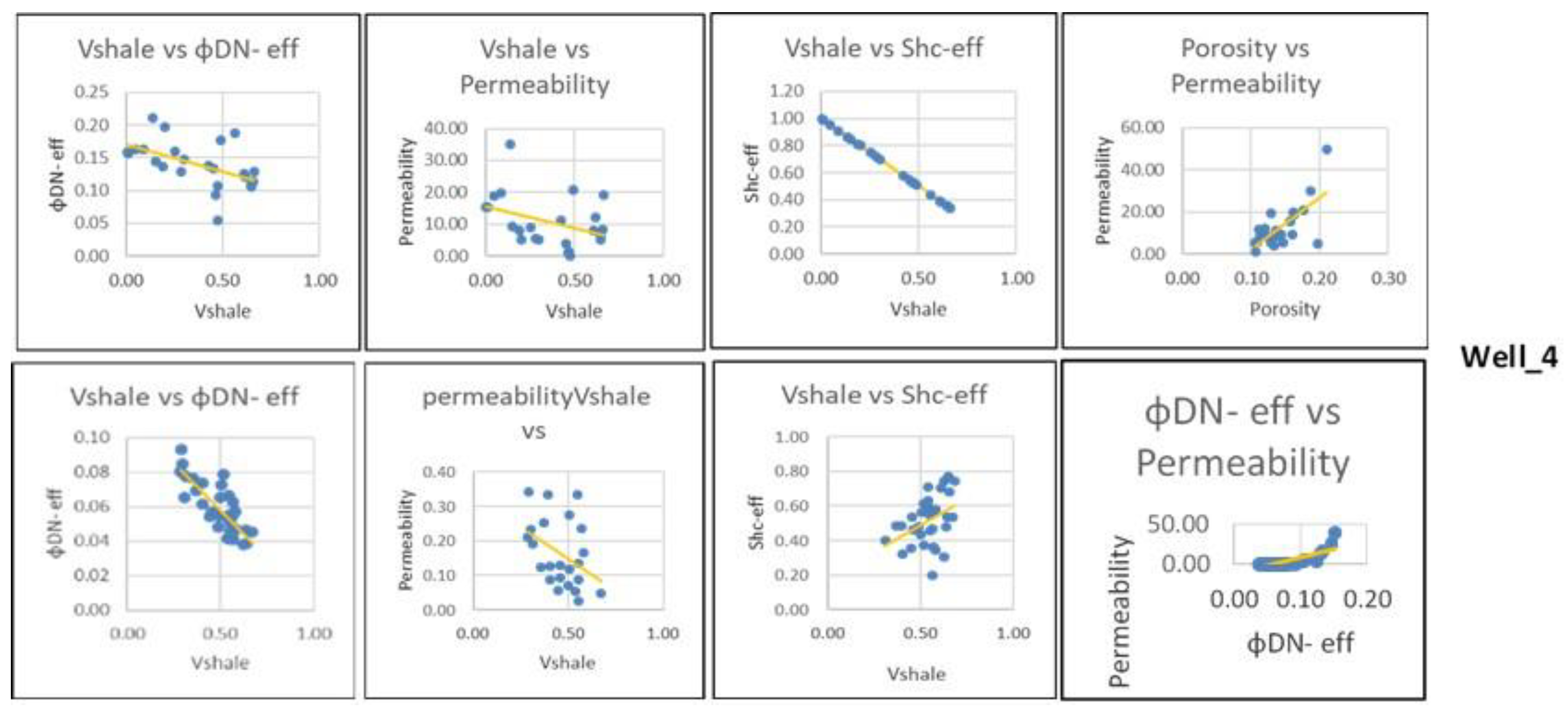
In Sand Dlower, porosity and permeability improve where Vsh is lower and effective porosity is higher (Figure 14). A clear negative correlation is evident between Vsh and reservoir quality indicators. Vsh remains a critical controlling factor, showing a strong inverse correlation with both porosity and permeability. The linear relationship between porosity and permeability is maintained.
In Sand E, porosity is higher in cleaner sands and reduced in zones with increased shale content (Figure 15. Permeability shows a rising trend with decreasing Vsh. Hydrocarbon saturation improves gradually with decreasing Vsh. Shale volume continues to negatively influence reservoir properties. A clear positive linear trend is observed between porosity and permeability.
In Sand F Porosity increases in sands with lower Vsh, (Figure 16). Hydrocarbon saturation shows a slight increase with improved porosity. Shale content remains a limiting factor for reservoir quality, and porosity-permeability correlation is positive and linear.
In Sand G, porosity increases with shale volume (Vsh) decrease, and permeability also improves (Figure 16), similar to Sand F. The negative influence of Vsh is evident, and a strong linear relationship exists between porosity and permeability.
From the above analysis, it becomes clear that D Sands are effectively the best reservoirs [32]. Sand Dupper shows good porosity, permeability, and Hydrocarbon saturation, all of them reducing in shale-rich zones, probably due also to poorer sorting. Sand Dlower presents good porosity and permeability in cleaner intervals in both wells, The consistency in these patterns reinforces the controlling influence of Vsh and depositional sorting on reservoir quality.
5. Results and Discussion
In previous works, Alam et al. [32] characterized the producing quality of three deep sandy zones (D-Upper, D-Lower and E-Sand) in three Srikail wells, based in Vsh, Porosity, Permeability and net-to-gross. Hossain et al. [33] also characterized three sandy units (named Zones 1, 2 and 3) in a single well (Srikail #3), indicating only average values for Vsh, Porosity, Water and Hydrocarbon Saturation, for each Zone. In this work, in-depth petrophysical evaluation and reservoir characterization of all the sandy intervals of the Srikail Gas Field was conducted through a combination of manual analysis and automated interpretation using Techlog software. Petrophysical parameters were derived through both empirical equations and software-based computations, and the results were compared to assess consistency and interpretation accuracy.
From the 11 previously identified reservoir zones (named A to K, from top to bottom), Srikail-1 well has intersected a total of nine reservoir layers (A to C and F to K) whereas Srikail-4 has intersected the seven reservoir layers (A to G), and both Srikail-2 and Srikail-3 wells only five (A to E).
The proportion of clay in reservoirs is a crucial parameter influencing its producing quality. The calculated average shale volume (Vshale) varies across different reservoir layers and among these, Zone C exhibits the highest shale content, whereas Zone B shows the lowest. Within each sandy interval, Vshale variability at specific depths indicates heterogeneous, interbedded sand-shale lithology from fluctuating depositional conditions. An overall increase in Vshale towards the top indicates a transition to finer-grained, lower-energy environments. This heterogeneity impacts reservoir quality by reducing porosity and permeability, affecting hydrocarbon flow.
Porosity estimation is a fundamental step in reservoir evaluation [34], and along with permeability, it dictates the fluid storage capacity and productivity of the reservoir (Dickey, 1986). Effective porosity was derived from a combination of effective density and neutron porosities. The overall effective porosity ranges from 4% to 20%. Sands A, B, D, and E exhibit favorable porosity values and are considered good quality reservoirs.
Hydrocarbon saturation (Shc) values further confirm reservoir potential. Based on the criteria of Asquith and Gibson [35], zones with Shc above 60% are considered hydrocarbon-bearing, making Zones A, B, D, and E the most promising. Zones C, F, G, H, I, J and K in contrast, demonstrate higher shale content, lower porosity, and limited hydrocarbon potential.
Mud log analysis revealed that C and G sands are highly calcareous with poor porosity. In Well-01, the G, H, I, J and K intervals also exhibited significant calcareous content [36] and sub-optimal porosity. Calcareous tests during mud logging and a lack of gas flow during DSTs (except in Sand I) suggest these sands have low permeability.
Permeability was estimated using the Timur equation for wells 1 through 4. D sands demonstrate the highest permeability and are already in production. Sands A, B, and E also show good permeability and are viable for hydrocarbon extraction. Zone E, in particular, is confirmed as a productive interval in Well-04. C and G sands have very poor permeability. Sands F, H, I, J and K show poor to moderate porosity and permeability, maybe producible with minimal stimulation (e.g. fracturing). Permeability values obtained from DST data in the deeper tested sands range from 0.6 to 0.01 mD [37], indicating a very tight reservoir with limited fluid flow capacity without stimulation.
Petrophysical parameters Cross Plots clearly point to an inverse relationship between Vshale and Porosity. Higher shale content corresponds with reduced porosity, as shale occupies pore spaces and obstructs pore throats. In this study, Zones C, G, F, H, I, J, and K are identified as low-quality reservoirs due to permeability, although some of them have good hydrocarbon saturation.
The relationship between Vshale, porosity, and permeability was further assessed. Both porosity and permeability decrease as Vshale increases. Cross-plotting porosity versus permeability reveals a strong linear correlation: well-sorted, clean sandstones with low shale content show high porosity and permeability. Conversely, zones with high clay content may display elevated porosity but reduced permeability due to matrix blockage. Considering that in most sands Vsh increases towards the upper layers, it may be concluded that permeability is lower on these more shaly layers. Moreover, the good correlation of Porosity decrease with Vhs increase allows us to consider that also Hydrocarbon saturation tends to decrease towards the upper layers. Overall, each sand tends to have better reservoir properties at its lower and intermediate layers, than at its upper more shaly layers.
Bulk Volume Water (BVW) values offer further insight into grain size and reservoir texture. According to Fertl and Vercellino [38], BVW values between 0.035 and 0.07 are indicative of fine to very fine-grained sands. The results (Table. 8) suggest that Sands A, B, and C are fine to very fine-grained, D sands are coarse-grained, and Sand E comprises fine-grained and silty material.
6. Conclusions
This research presents an integrated petrophysical evaluation and reservoir characterization of the Srikail Gas Field, utilizing both manual techniques and advanced digital interpretation through Techlog software. A combination of digital and hardcopy well log data was used to estimate essential petrophysical properties such as shale volume, porosity, fluid saturation, permeability, and bulk volume of water (BVW). The study employed empirical cross-plots, analytical models, and automated processing to improve the precision and consistency of interpretations. A quick-look methodology aided in identifying key reservoir intervals and gas-bearing zones.
The analysis reveals that reservoir quality within the field varies from poor to good. Net reservoir thicknesses range from 8 to 66 meters, with shale content between 31% and 83%. Effective porosity spans from 4% to 20%, hydrocarbon saturation ranges from 54% to 96%, and effective water saturation falls between 4% and 46%. Permeability estimates vary widely from 0.05 to 355 mD, while BVW values are between 0.02 and 0.08.
Both qualitative and quantitative interpretations were carried out to assess the characteristics of individual reservoir layers. The identified reservoirs predominantly consist of shaly sandstones. Reservoirs A, B, and E show moderate to good reservoir properties, characterized by fine to very fine-grained, silty sandstones with fair to good permeability. Conversely, Reservoirs C and G exhibit poor quality, highly calcareous composition (from mud logging) and extremely low permeability, consistent with tight sandstone classification. Deeper sands such as F, H, I, J, and K display tight to semi-conventional characteristics and are likely to benefit from targeted stimulation and advanced completion strategies.
The most productive zones - Upper D and Lower D - are identified by their cleaner and coarser grain size and superior permeability, contributing significantly to gas production. Meanwhile, DST-derived permeability values from deeper sands (e.g., G, H, J) confirm extremely tight conditions, ranging from 0.6 to 0.01 mD.
Regardless of the different sands and burial depths, there is a clear pattern of upwards decrease in hydrocarbon production properties towards the top layers of each producing sand. This fact indicates the importance of initial sandy inputs, gradually “contaminated” by clay inputs into the depositional environment. In other words, each sand seems to represent a 4th order finning upwards cycle [39].
Integrating the previous analysis, Reservoir Zones A, B, D, and E clearly appear as high-quality reservoirs due their favorable porosity, permeability, hydrocarbon saturation, and low shale content. Among these, D and E sands are already productive, supporting their classification as effective hydrocarbon-bearing reservoirs. In contrast, Zones C and G exhibit poor reservoir characteristics and may be classified as tight sands due to their calcareous nature, poor porosity and limited permeability. On the other hand, F, H, I, J, and K are tight to semi-conventional and might require partial stimulation and proper completion.
To improve future reservoir understanding and development, it is recommended that further studies incorporate core analysis and 3D seismic data in conjunction with petrophysical log interpretation. This integrated approach will provide a more comprehensive insight into reservoir heterogeneity and enhance resource recovery strategies across the Srikail Gas Field.
Acknowledgments
BAPEX (Bangladesh Petroleum Exploration & Production Company Ltd.) is highly acknowledged by the authors for the access and use of the various data sets used for this work, particularly the wire-line logs and mud logs of the Srikail gas field wells. The Department of Geology and the Instituto Dom Luiz, both at the Faculty of Sciences of Lisbon University, are acknowledged by the authors for their IT and logistical assistance during this work. Schlumberger is acknowledged for the use of an academic license of Techlog used to analze all the wireline logs.
References
- Zeba, J.; Murrell, R. Evaluation of Rock Properties from Logs Affected by Deep. Unpublished Manuscript, 2015.
- Simandoux, P. Mesures Dielectriques en Milieu Poreux, Application à Mesure des Saturations en Eau, Étude du Comportement des Massifs Argileux. Rev. Inst. Fr. Pétrol.
- Poupon, A.; Leveaux, J. Evaluation of Water Saturations in Shaly Formations. Log Analyst 1971, 12, 4. [Google Scholar]
- Islam, M.S.; Islam, M.R.; Hossain, M.A.; Rahman, A.M. Petrophysical Analysis of Shaly Sand Gas Reservoir of Titas Gas Field Using Well Logs. Bangladesh J. Geol. 2006, 25, 106–124. [Google Scholar]
- Islam, M.D.; Rahman, M.D.; Woobaidullah, A.S.M. Reservoir Characterization of Srikail Gas Field Using Wireline Log Data. D.U. J. Earth Environ. Sci. 2018, 5. [Google Scholar]
- Islam, A.R.M.T.; Islam, M.A. Evaluation of Gas Reservoir of the Meghna Gas Field, Bangladesh Using Wireline Log Interpretation. Univ. J. Geosci. 2014, 2, 62–69. [Google Scholar] [CrossRef]
- Islam, A.R.; Islam, T.; Biswas, R.; Jahan, K. Petrophysical Parameter Studies for Characterization of Gas Reservoir of Narsingdi Gas Field, Bangladesh. Int. J. Adv. Geosci. 2014, 2, 53–58. [Google Scholar]
- Mostafizur, R.; Woobaidullah, A.S.M. Evaluation of Reservoir Sands of Habiganj-7 Well by Wireline Log Interpretation. D.U. J. Earth Sci. 2010.
- Reimann, K.U. Geology of Bangladesh; Gebrüder Borntraeger: Berlin, Germany, 1993; p. 160. [Google Scholar]
- Banglapedia. National Encyclopedia of Bangladesh; Asiatic Society of Bangladesh: Dhaka, Bangladesh, 2003. [Google Scholar]
- Alam, M. Geology and Depositional History of Cenozoic Sediments of the Bengal Basin of Bangladesh. Palaeogeogr. Palaeoclimatol. Palaeoecol. 1989, 69, 125–139. [Google Scholar] [CrossRef]
- Curray, J.R.; Emmel, F.J.; Moore, D.G.; Raitt, R.W. Structure, Tectonics, and Geological History of the Northeastern Indian Ocean. In The Ocean. In The Ocean Basins and Margins; Nairn, A.E.M., Stehli, F.G., Eds.; Springer: Boston, MA, USA, 1982; pp. 399–450. [Google Scholar]
- Alam, M.; Alam, M.M.; Curray, J.R.; Chowdhury, M.L.R.; Gani, M.R. An Overview of Sedimentary Geology of the Bengal Basin in Relation to the Regional Tectonic Framework and Basin Fill History. Sediment. Geol. 2003, 155, 179–208. [Google Scholar] [CrossRef]
- Evans, P. Tertiary Succession in Assam. Trans. Mineral. Geol. Inst. India 1932, 27, 155–260. [Google Scholar]
- Alam, M.M. Sedimentology and Depositional Environment of Subsurface Neogene Sediments in the Sylhet Trough, Bengal Basin: Case Study of the Fenchuganj and Beanibazar Structures, Northeastern Bangladesh. Unpublished report, Bangladesh Petroleum Institute, 1993, 1–82.
- Holtrop, J.F.; Keizer, J. Some Aspects of the Stratigraphy and Correlation of the Surma Basin Wells, East Pakistan. ECAFE Mineral Resour. Dev. Serv. 1970, 36, 143–154. [Google Scholar]
- Hiller, K.; Elahi, M. Structural Growth and Hydrocarbon Entrapment in the Surma Basin, Bangladesh. In Petroleum Resources of China and Related Subjects; Wagner, H.C., Wagner, L.C., Wang, F.F.H., Wong, F.L., Eds.; Circum-Pacific Council for Energy and Mineral Resource Earth Science Series, 1988, 10, 657–669. [Google Scholar]
- Banerjee, M.; Sen, P.; Dastidar, A.G. On the Depositional Condition of the Holocene Sediments of Bengal Basin with Remarks on Environmental Condition of the Soft Grey Clay Deposition in Calcutta. Proc. Indian Geotech. Conf. 1984, 1(Div. I), 63–69. [Google Scholar]
- Johnson, S.; Alam, A. Sedimentation and Tectonics of the Sylhet Trough, Bangladesh. Geol. Soc. Am. Bull. 1991, 103, 1513–1527. [Google Scholar] [CrossRef]
- Sultana, D.N.; Alam, M.M. Facies Analysis of the Neogene Surma Group Succession in the Subsurface of the Surma Basin, Bengal Basin, Bangladesh. Bangladesh Geosci. J. 2001, 6, 53–74. [Google Scholar]
- Bangladesh Petroleum Exploration and Production Company Limited (BAPEX). Well Completion Reports of Srikail #1, #2, #3, and #4. Unpublished report.
- Petrobangla. Srikail Geological Study. Petrobangla: Dhaka, Bangladesh, 2009. Unpublished report.
- Rider, M.H. The Geological Interpretation of Well Logs; Whittles Publishing: Caithness, UK, 2000. [Google Scholar]
- Schlumberger. Log Interpretation Principles/Applications; Schlumberger: Houston, TX, USA, 1989. [Google Scholar]
- Schlumberger. Log Interpretation Charts: English Metric; Schlumberger: Houston, TX, USA, 1979. [Google Scholar]
- Schlumberger. Log Interpretation. Vol. II: Applications; Schlumberger Well Services Inc.: Houston, TX, USA, 1974. [Google Scholar]
- Schlumberger. Log Interpretation. Vol. I: Principles; Schlumberger Well Services Inc.: Houston, TX, USA, 1972. [Google Scholar]
- Nawab, M.M.; Islam, M.A. Estimation of Shale Volume Using Gamma and Porosity Logs: Application to the Selected Gas Fields of Bangladesh. Bangladesh Geosci. J. 2005, 11, 89–99. [Google Scholar]
- Markel, R.H. Well Log Formation Evaluation; AAPG Continuing Education Course Note Series: Tulsa, OK, USA, 1979; Volume 14, p. 82. [Google Scholar]
- Archie, G.E. The Electrical Resistivity Log as an Aid in Determining Some Reservoir Characteristics. Petrol. Tech. 1942, 5, 54–62. [Google Scholar] [CrossRef]
- Worthington, P.F. The Evolution of Shaly-Sand Concepts in Reservoir Evaluation. Log Analyst 1985, 23, 1. [Google Scholar]
- Alam, K.; El-Husseiny, A.; Abdullatif, O.; Babalola, L. Petrophysical Evaluation of Prospective Reservoir Zones in Srikail Gas Field, Bengal Basin Bangladesh. 81st EAGE Conf. Exhib. 2019, 2019, 1–5. [Google Scholar]
- Hossain, D.; Rahman, M.; Khatu, H.; Haque, R. Petrophysical Properties Assessment Using Wireline Logs Data at Well #3 of Srikail Gas Field, Bangladesh. China Geol. 2022, 5, 393–401. [Google Scholar]
- Ruhovets, N. A Log Analysis Technique for Evaluating Laminated Reservoirs in the Gulf Coast Area. Log Analyst 1990, 31, 294–303. [Google Scholar]
- Asquith, G.B.; Gibson, C. Basic Well Log Analysis for Geologists; AAPG: Tulsa, OK, USA, 1982; p. 216. [Google Scholar]
- Bangladesh Petroleum Exploration and Production Company Limited (BAPEX). Report on Technical Study for Possibility of Re-Entry/Re-Visit the Suspended, Dry & Abandoned Wells under BAPEX (Case Study: Srikail Gas Field), 20. Unpublished report. 20 August.
- Bangladesh Petroleum Exploration and Production Company Limited (BAPEX). Final Technical Report on Srikail Field (3D Project of BAPEX), Schlumberger. Unpublished report.
- Fertl, W.H. Shaly-Sand Analysis in Development Wells. In Proc. 16th Ann. Logging Symp.; Soc. Prof. Well Log Analysts: Houston, TX, USA, 1975. [Google Scholar]
- Akhter, S.; Pimentel, N. Sequence Stratigraphy of Miocene Deltaic Sands in the Srikail Gas Field, East-Central Bengal Basin: Insights from Mud Log and Wireline Log Data. J. Geol. Soc. India.
Figure 1.
Regional and local Tectonic Elements of Bengal Basin (adapt. from Reimann 1993). Numbers 1 to 10 indicate the different sub-basins and the Srikail Gas Field is located in the Surma sub-basin (Number 7).
Figure 1.
Regional and local Tectonic Elements of Bengal Basin (adapt. from Reimann 1993). Numbers 1 to 10 indicate the different sub-basins and the Srikail Gas Field is located in the Surma sub-basin (Number 7).
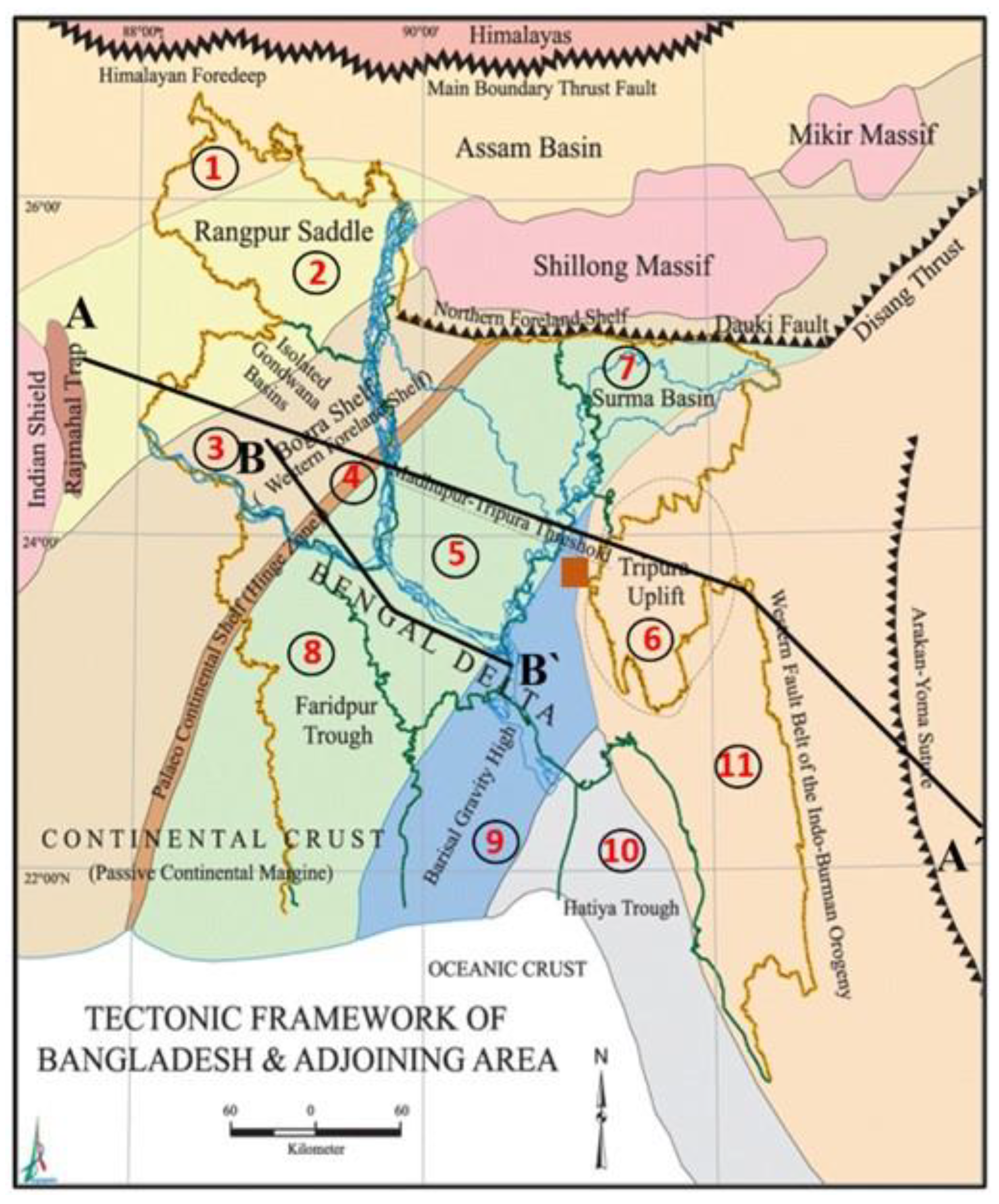
Figure 2.
(see Figure 1 for location): A) Regional geotectonic cross-section for the Bengal Basin (adapt. from Alam et al. 2003); B) Regional cross-section of the Tertiary sedimentary infill of the Bengal basin (Alam et al. 2003), showing thicker units to the SE, where the Srikail field is located.
Figure 2.
(see Figure 1 for location): A) Regional geotectonic cross-section for the Bengal Basin (adapt. from Alam et al. 2003); B) Regional cross-section of the Tertiary sedimentary infill of the Bengal basin (Alam et al. 2003), showing thicker units to the SE, where the Srikail field is located.
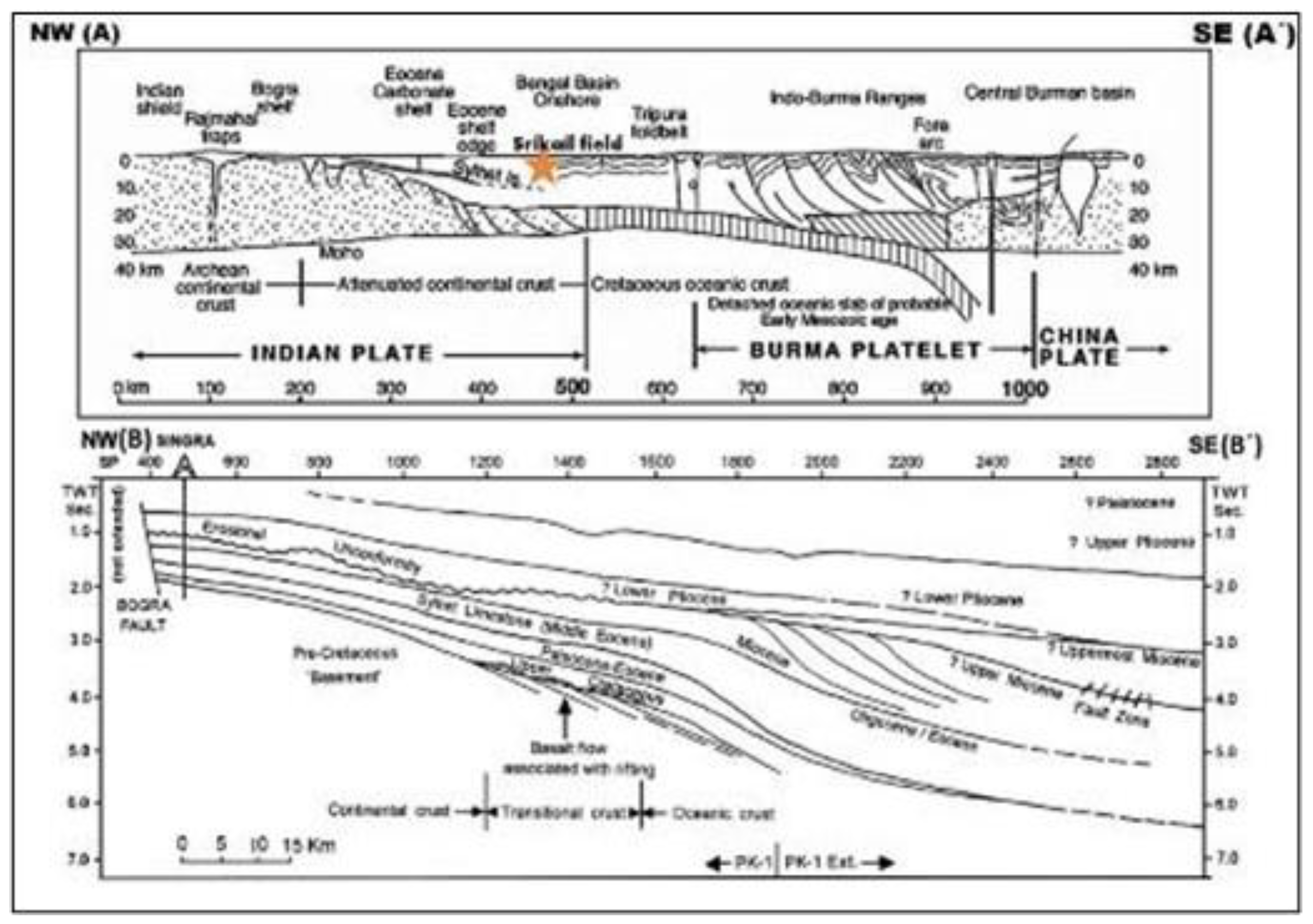
Figure 3.
General Stratigraphy of the study area (modified from Alam et al. 2003).
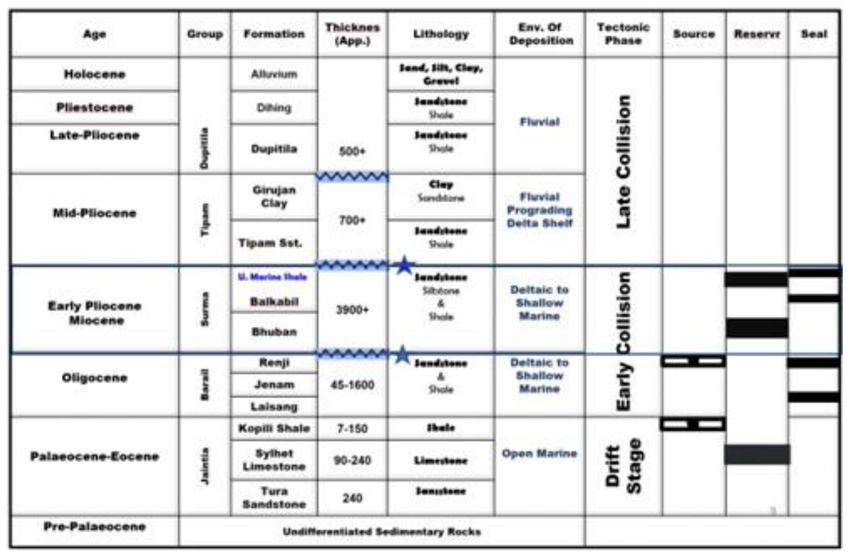
Figure 4.
Srikail wells geographical location and position in BAPEX seismic line grid.
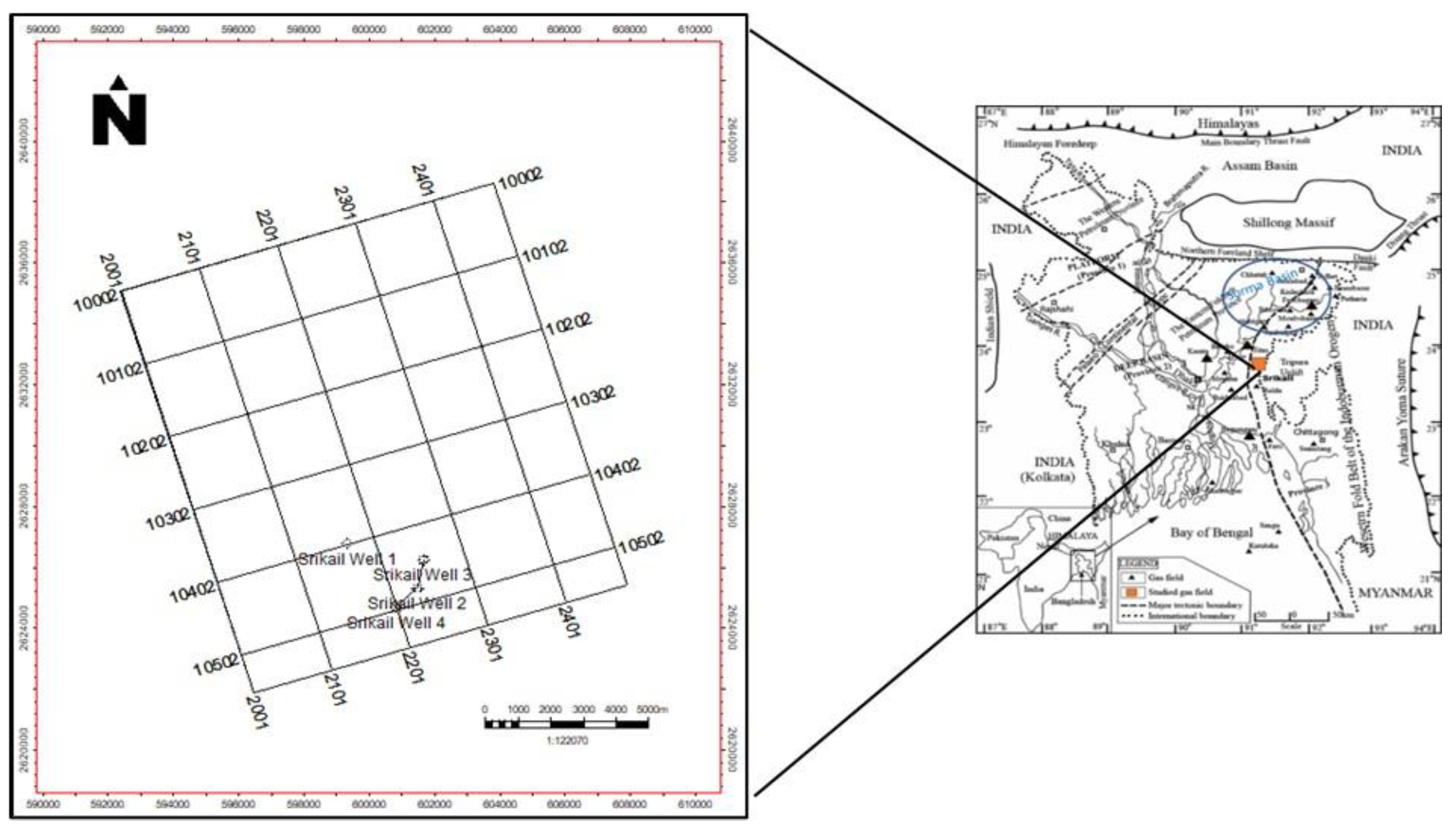
Figure 5.
Petrophysical results (Techlog) for F, G, H, I, J and K Sands in Well 1.
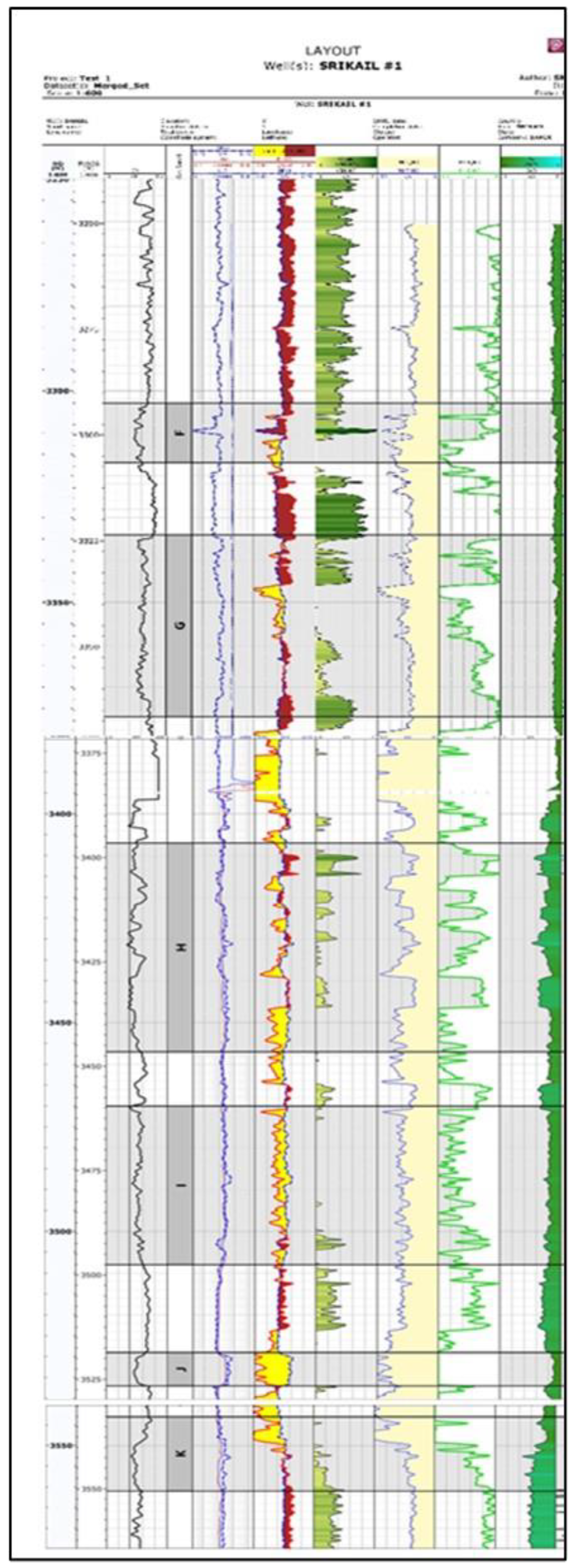
Figure 6.
Petrophysical results (Techlog) for C, Dup, D low, and E Sands in Well 2.
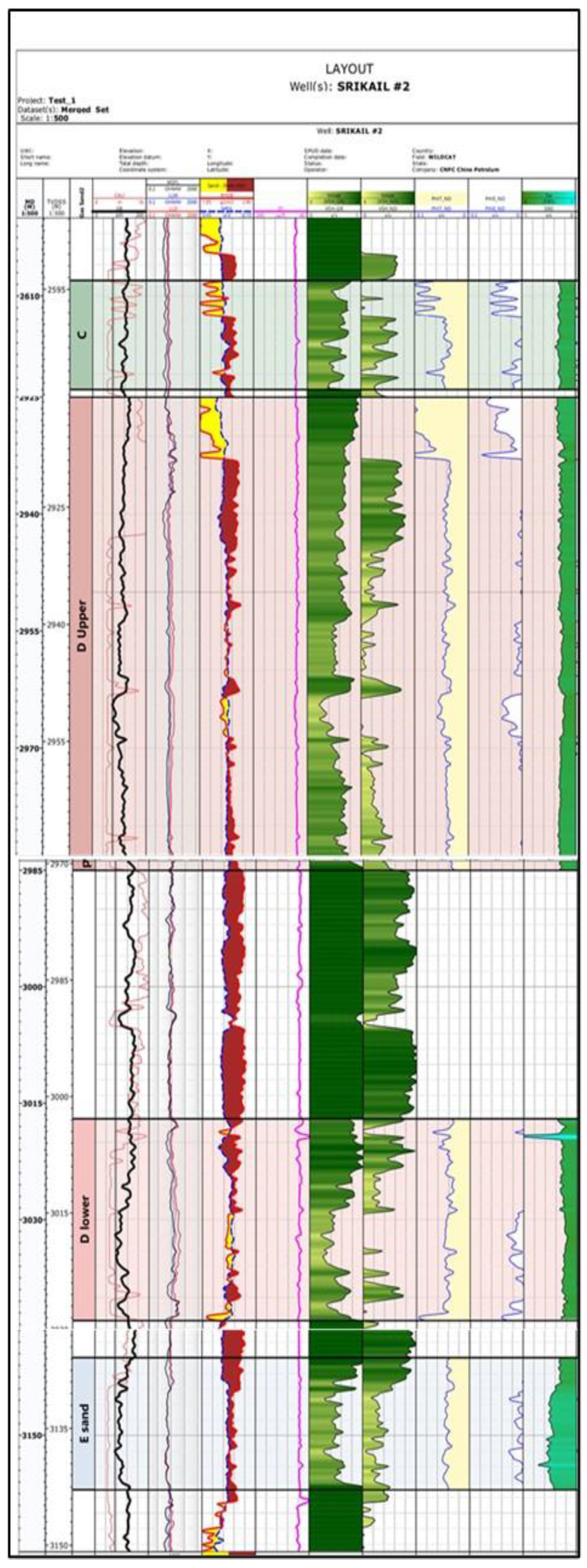
Figure 7.
Petrophysical results (Techlog) for C, Dup, D low, and E Sands in Well 3.
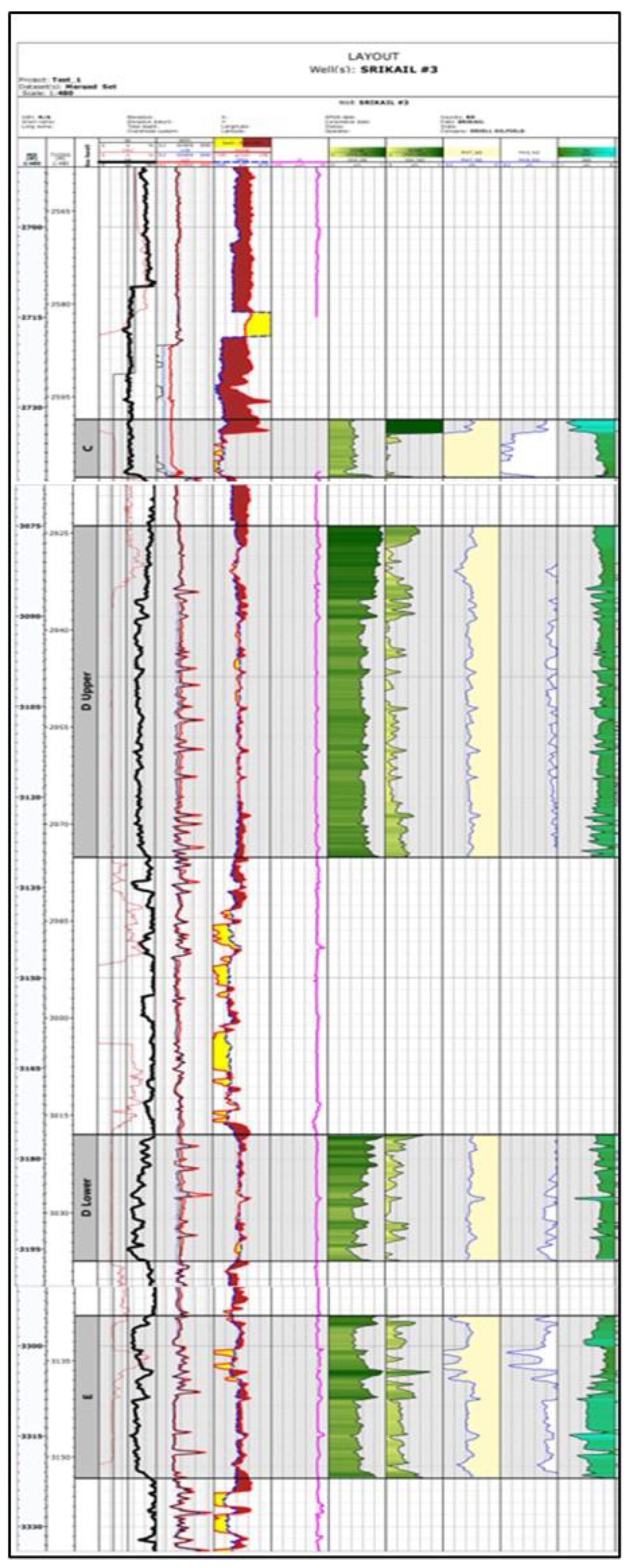
Figure 8.
Petrophysical results (Techlog) for C, Dup, D low, and E Sands in Well 4.
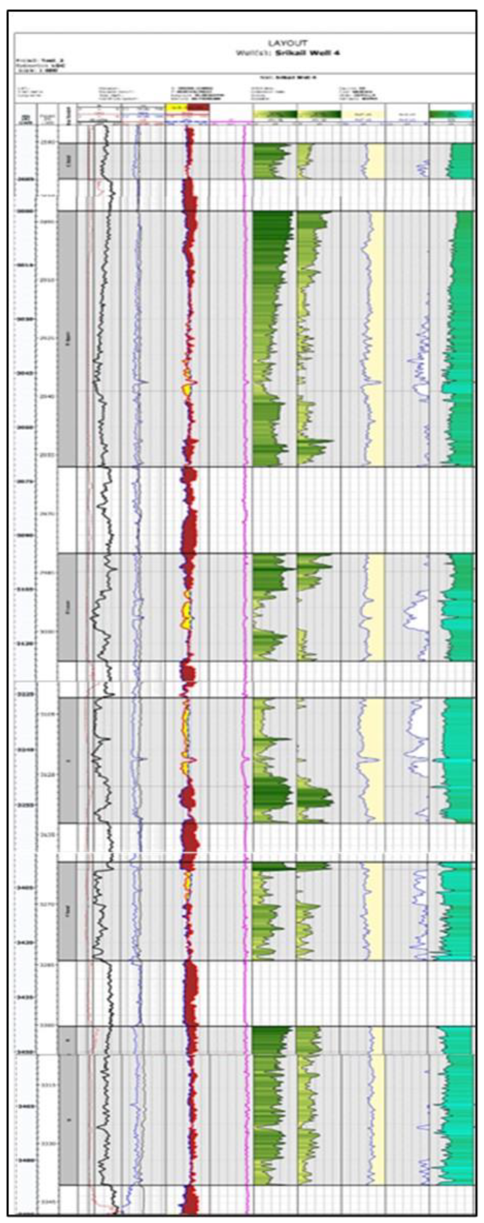
Figure 9.
Vsh variation with Depth for Sands (A, B, C, Dup, Dlow and E) in well 2 and 4.
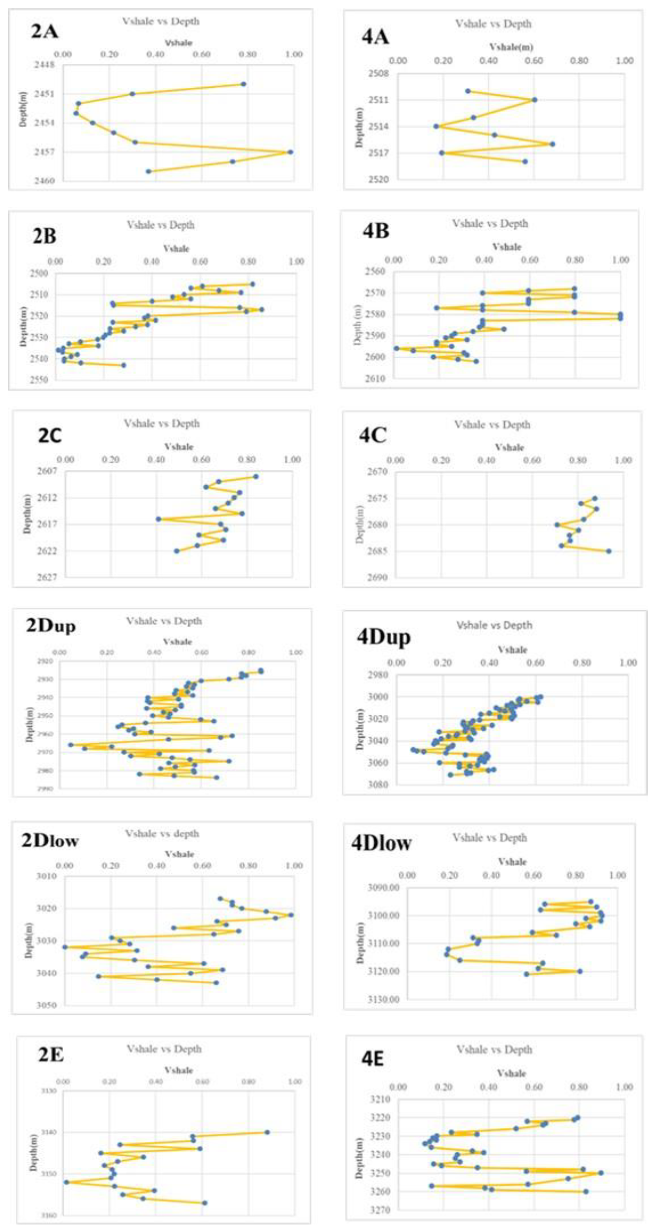
Figure 10.
Cross plots of Sand A.
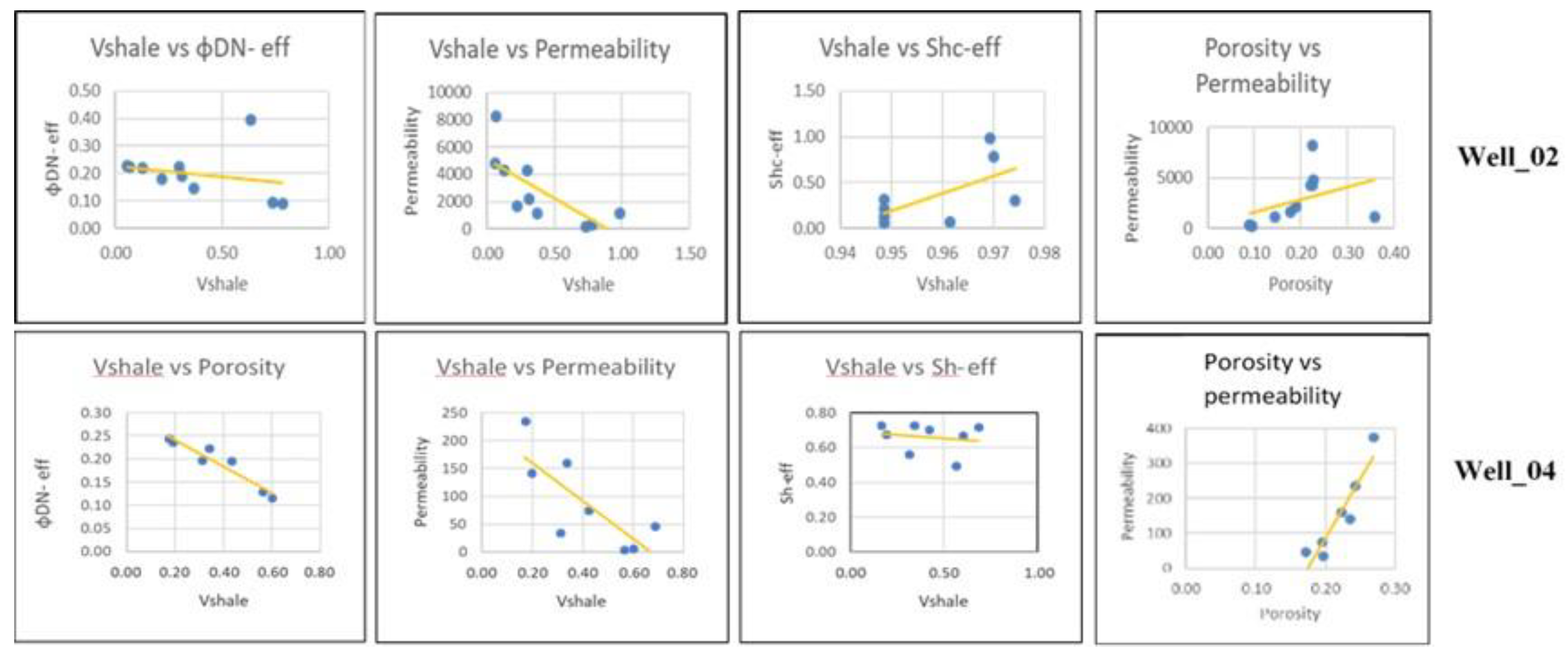
Figure 11.
Cross plots of Sand B.
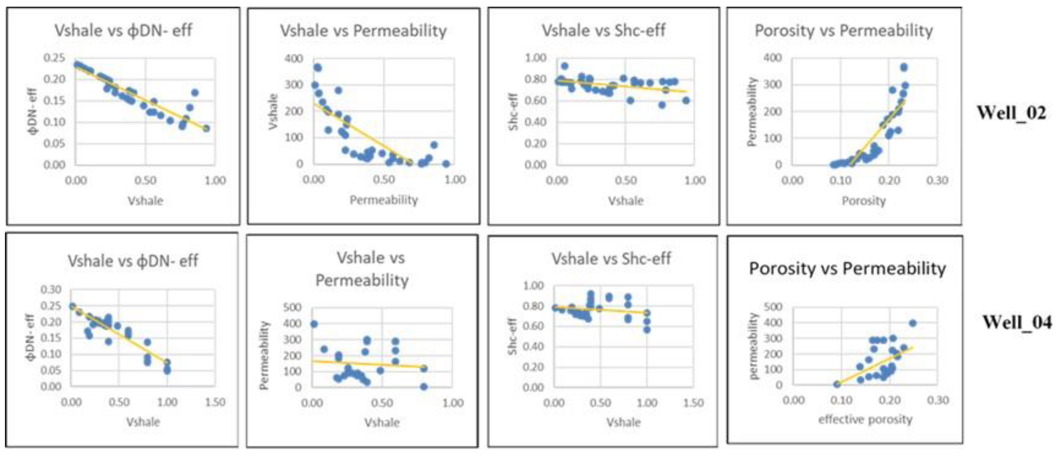
Figure 12.
Cross plots of Sand C.
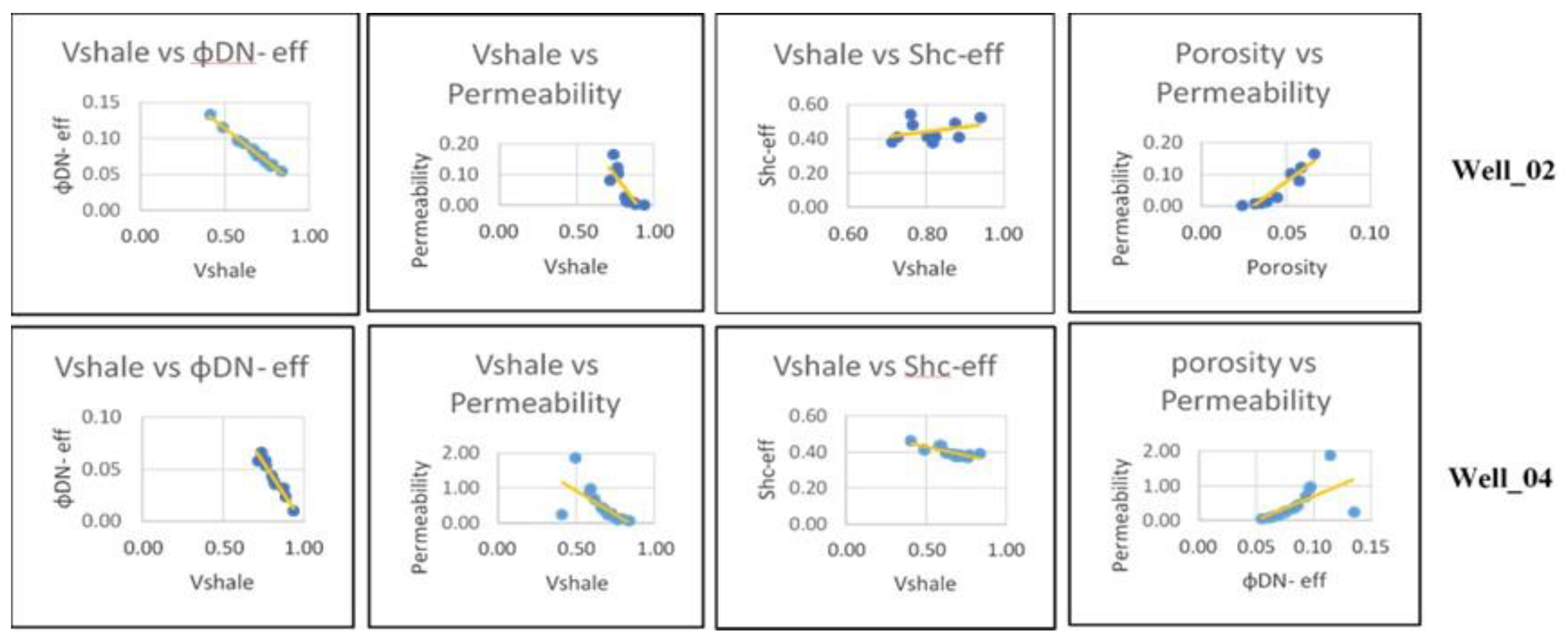
Figure 13.
Cross plot of Sand Dupper.
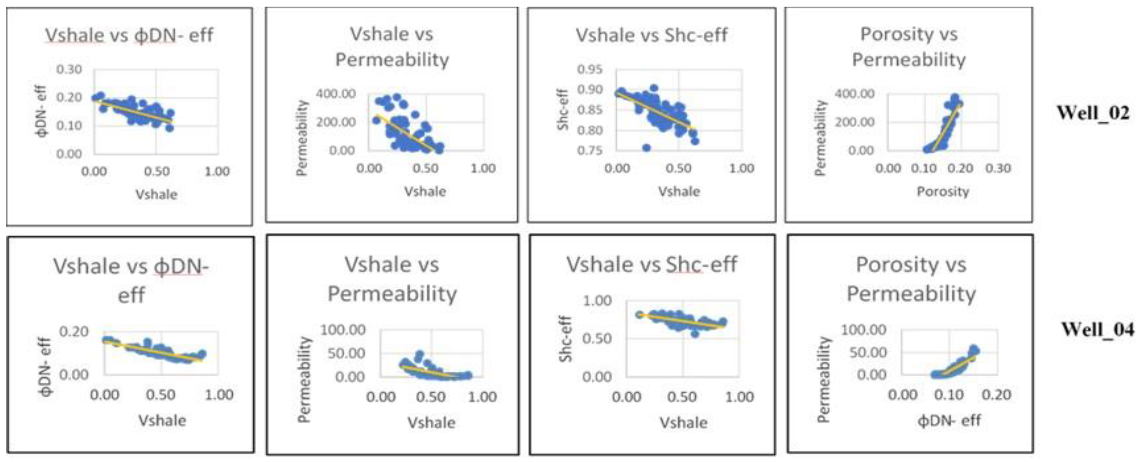
Figure 14.
Cross plot of Sand Dlower.
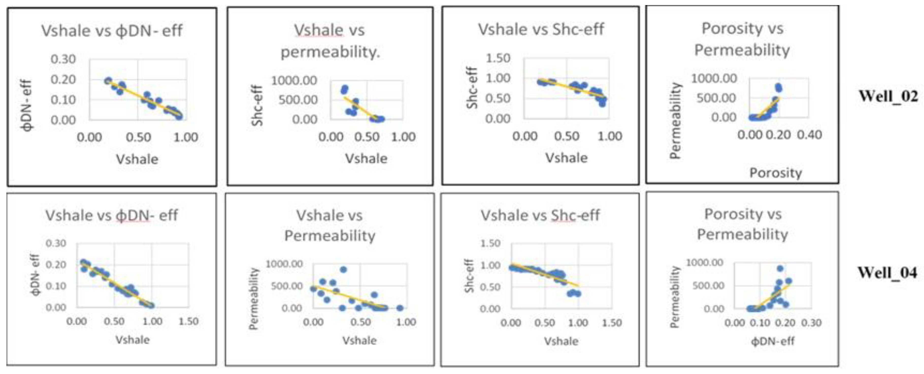
Figure 15.
Cross plot of Sand E.
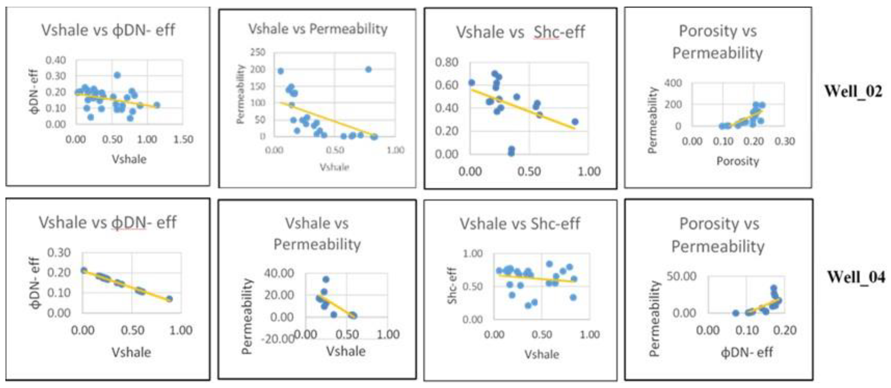
Figure 16.
Cross plot Sand F and G.
| Well Name | Total Depth | Identified Reservoir zones | |
| MD | TVDSS | ||
| Srikail Well_1 | 3583m | 3572m | A, B, C, F, G, H, I, J, K |
| Srikail Well_2 | 3214m | 3198m | A, B, C, Dup, Dlower, E |
| Srikail Well_3 | 3350m | 3178m | A, B, C, Dup, Dlower, E |
| Srikail Well_4 | 3512 | 3360m | A, B, C, Dup, Dlower, E, F, G |
Table 2.
Thickness of Reservoir zones.
| Zone | Well_1 | Well_2 | Well_3 | Well_4 | |
| A | 11m | 11m | 10m | 08m | |
| B | 31m | 38m | 35m | 33m | |
| C | 24m | 14m | 14m | 10m | |
|
D |
Dupper | - - |
60m | 52m | 66m |
| Dlower | 26m | 20m | 27m | ||
| E | - | 17m | 26m | 37m | |
| F | 15m | - | - | 24m | |
| G | 39m | - | - | 40m | |
| H | 18m | - | - | - | |
| I | 38m | - | - | - | |
| J | 08m | - | - | - | |
| K | 15m | - | - | - | |
Table 3.
Openhole composite logs.
| Hole Section | Scale | Description |
| 12.25" | 1:200/1:500/1:1000MD | Composite-Log |
| 12.25" | 1:200/1:500/1:1000MD | GR/SP/Resistivity |
| 12.25" | 1:200/1:500/1:1000MD | Density/Porosity/Cali/GR |
| 12.25" | 1:200MD | Composite Plot |
| 8.5" | 1:200/1:500/1:1000MD | Composite-Log |
| 8.5" | 1:200/1:500/1:1000MD | GR/SP/Resistivity |
| 8.5" | 1:200/1:500/1:1000MD | Density/Porosity/Cali/GR |
| 8.5" | 1:200MD | Full wave sonic/GR |
Disclaimer/Publisher’s Note: The statements, opinions and data contained in all publications are solely those of the individual author(s) and contributor(s) and not of MDPI and/or the editor(s). MDPI and/or the editor(s) disclaim responsibility for any injury to people or property resulting from any ideas, methods, instructions or products referred to in the content. |
© 2025 by the authors. Licensee MDPI, Basel, Switzerland. This article is an open access article distributed under the terms and conditions of the Creative Commons Attribution (CC BY) license (https://creativecommons.org/licenses/by/4.0/).
Copyright: This open access article is published under a Creative Commons CC BY 4.0 license, which permit the free download, distribution, and reuse, provided that the author and preprint are cited in any reuse.


