Control Sets of Linear Control Systems on 2-Dimensional Lie Groups. Examples

1. Introduction

Let M be a finite-dimensional differential manifold. A control system in M is defined by the family of ordinary differential equations (ODEs),

$$\dot{x}\left(t\right)=f_0\left(x\left(t\right)\right)+\sum _{j=1}^m{u}_j\left(t\right)f_j\left(x\left(t\right)\right),u\in \mathcal{U},\left({\mathsf{\Sigma }}_M\right)$$

determined by $u=(u_1,\dots ,u_m)$ in $\mathcal{U}$, the set of the admissible class of piecewise constant functions, with $u\left(t\right)\in \mathsf{\Omega }$. The set $\mathsf{\Omega }\subset {\mathbb{R}}^m$ is a closed and convex subset of the m-dimensional Euclidean space with $0\in int\left(\mathsf{\Omega }\right)$. When $\mathsf{\Omega }={\mathbb{R}}^m$ the system is called unrestricted. We consider the restricted case, i.e., when $\mathsf{\Omega }$ is compact.

Here, $f_0,f_1,\dots ,f_m$ are smooth vector fields on M, $f_0$ is referred to as the drift, while $f_1,\dots ,f_m$ are the control vectors that influence the drift.

For any $x\in M$ and $u\in \mathcal{U}$ the solution of ${\mathsf{\Sigma }}_M$ is the integral curve $t\mapsto \varphi (t,x,u)$ on M satisfying $\varphi (0,x,u)=x$. The positive and negative orbits of ${\mathsf{\Sigma }}_M$ at x are defined as follows,

$${\mathcal{O}}^{+}\left(x\right)=\{\varphi (t,x,u),t\ge 0,u\in \mathcal{U}\}\mathrm{and}{\mathcal{O}}^{-}\left(x\right)=\{\varphi (-t,x,u),t\ge 0,u\in \mathcal{U}\},$$

respectively. We say that ${\mathsf{\Sigma }}_M$ satisfies the Lie Algebra Rank Condition (LARC) if the Lie algebra $\mathcal{L}$ generated by the vector fields $f_0,f_1,\dots ,f_m$, satisfies

$$\mathcal{L}\left(x\right)=T_{x}M\mathrm{for}\mathrm{all}x\in M.$$

It is well known that the Lie Algebra Rank Condition (LARC) assures that the positive and negative orbits of the system have non-empty interiors. The system ${\mathsf{\Sigma }}_M$ is said to be controllable if $M={\mathcal{O}}^{+}\left(x\right)$ for all $x\in M$. Controllability is a powerful property of a control system. It means that given an initial condition x and a desired final state y, there exists a control u such that the associated integral curve $\varphi (t,x,u)$ corresponding to the ordinary differential equation determined by u transfers the first state to the second one over a positive time interval, i.e., $\varphi (0,x,u)=x$ and $\varphi (T,x,u)=y$ for some positive time T. This property is essential, for instance, when addressing optimization problems, such as minimal time issues, maximum profit, minimum cost of energy, minimum collateral damage, etc. In fact, to establish the existence of a minimum time curve connecting two states, it must first be demonstrated that at least one connecting curve exists. The Chow-Rashevskii Theorem [1,19], states that if the LARC is satisfied, then there exists a metric defined on the manifold M. Specifically, any two states on M can be connected by a curve formed through vector fields in the Lie algebra of the system. The Lie brackets take into account both positive and negative time, which can not be considered in this contex.

Achieving controllability can be quite challenging, even for specific control systems acting on analytical manifolds with additional structures, like Lie groups. In the next section, we will describe the Kalman rank condition, which characterizes controllability for classical linear control systems in Euclidean spaces. It is important to note that this condition is based on the assumption that the set $\mathsf{\Omega }={\mathbb{R}}^m$, which is often unrealistic. The problem is mathematically well-posed, allowing for the determination of the limits one can expect in the restricted process. Additionally, when the control range set is bounded, the Kalman rank condition, combined with certain requirements regarding the spectrum of the drift, can offer valuable insights into controllability.

Let G be a Lie group with Lie algebra $\mathfrak{g}$. Since the landmark paper by R. W. Brockett, titled “System Theory on Group Manifolds and Coset Spaces,” published in 1972, the concept of controllability has been explored in the context of control systems on Lie groups [12].

There are two main categories of systems defined on Lie groups, distinguished by their dynamics, which arise from Abelian, nilpotent, solvable, and semisimple Lie algebras [18]. Invariant systems and linear systems. For a through understanding of invariant systems, where the drift and control vectors are elements of $\mathfrak{g}$ considered as left-invariant vector fields, we refer to Y. Sachkov’s survey, “Controllability of Invariant Systems on Lie Groups and Homogeneous Spaces" which summarizes results from over 40 years of research [27].

On the other hand, when the drift is linear, i.e. when its flows is a one-parameter group of G-automorphisim, and the control vectors are element of the Lie algebra $\mathfrak{g}$, we arrive at the definition of Linear control systems initially established for matrix groups [25], and subsequently generalized for any Lie group in [2].

In the context of Lie groups, the dynamical behavior of LCSs has been extensively studied by utilizing the inherent geometric richness found within Lie groups. See [3,6,7,14,21] and references therein. In that work, the significance of this extension is demonstrated through an equivalence theorem that, in simple terms, establishes a fundamental relationship: any control-affine system on a connected manifold, as ${\mathsf{\Sigma }}_M$, whose associated vector fields are complete and generate a finite Lie algebra is diffeomorphic equivalent to a LCS on a homogeneous space [20]. Which is the reason why we intend to submit a manuscript for LCS on this kind of special manifolds.

For more recent developments related to linear control systems, please consult [3,6,7,9].

Next, we introduce the notion of a control set, which is a region of the state space where controllability holds in its interior. In the sequel, the term “maximal” will refer to set inclusion. Additionally, $cl\left(P\right)$ will denote the topological closure of a set P.

Definition 1.

A set $\mathcal{C}\subset M$ is acontrol setof ${\mathsf{\Sigma }}_M$ if it is maximal with respect to the following properties:

1.

For every $x\in \mathcal{C}$, there exits $u\in \mathcal{U}$ such that $\varphi ({\mathbb{R}}_{+},x,u)\subset \mathcal{C}$;

2.

For every $x\in \mathcal{C}$, it holds that $\mathcal{C}\subset cl\left({\mathcal{O}}^{+}\left(x\right)\right)$.

For general control systems defined on manifolds, several papers have focused on the existence, uniqueness, and topological properties of control sets [14,15,28]. Precisely, assume the control system satisfies LARC and let $\mathcal{C}$ be a control set with non-empty interior. It holds,

• $\mathcal{C}$ is connected and $cl\left(int\mathcal{C}\right)=cl\left(\mathcal{C}\right)$;
• $int\mathcal{C}\subset {\mathcal{O}}^{+}\left(x\right)$.
• For any $x\in int\mathcal{C}$ it follows that,

  $$\mathcal{C}=cl\left({\mathcal{O}}^{+}\left(x\right)\right)\cap {\mathcal{O}}^{-}\left(x\right).$$

It turns out that the controllability property holds in $int\mathcal{C}$. Extending this framework to the class of LCS defined on Lie groups—which naturally generalize classical linear systems—our approach considers control sets as subsets of the state space where controllability holds.

In this survey, we review the literature that explicitly exhibits control sets with and without non-empty interiors. Our focus is on the class of linear control systems on two-dimensional Lie groups and their homogeneous spaces. We provide a comprehensive overview of these control sets, which include classical linear systems on the plane, as well as a linear control system on the two-dimensional solvable Lie group G. The results come from several papers produced by our research team, including: [4,5,16,17]. On the other hand, we include several application models. Specific examples include a planar drivetrain with a neutral mode, a planar servo with antagonist damping, a lightly damped oscillator with complex eigenvalues, and linear control on $Af{f}_{+}\left(2\right)$ demonstrating global controllability. The study also extends to applications in neuroscience, modeling orientation dynamics in the primary visual cortex (V1). Depending on parameters such as decay and modulation, the control sets range from complete controllability to conic or fiber-like regions, capturing the limits of mutual reachability in the state space. The results have practical implications for robotics, automation, and understanding cortical response properties.

The paper is organized as follows. In Section 2, we introduce the concepts of linear and invariant vector fields on a connected Lie group G. Section 3 presents the definition of Linear Control Systems (LCSs) on Lie groups and discusses controllability, specifically when the control set is the entire state space. We begin with the classical LCS on Euclidean spaces, detailing the general solution’s form and the Kalman condition for controllability. Next, we explain how to generalize the drift and control vectors from Euclidean spaces to Lie groups. We then introduce the definition of an LCS on G and present the features of its general solution. Section 4 discusses the control sets for classical LCSs in the plane, which vary based on the nature of the eigenvalues of the drift matrix A. Here, the determinant $\det A$ and the trace $\mathrm{tr}A$ are instrumental, [4,5]. In Section 5, we introduce in coordinates the general form of an LCS on the solvable Lie group of dimension two $G={\mathrm{Aff}}_{+}\left(2\right)$, and identify all control sets. Finally, in Section 6, we include several application models.

2. Preliminaries

Definition 2.

A Lie group is a differentiable manifold G with a group structure, such that the analytical product and inverse maps, denoted by μ and I, reads as follows

$$\begin{array}{ccccc}\mu :\hfill & G\times G⟶G\hfill & & I:\hfill & G⟶G\hfill \\ & (g,h)⟼\mu (g,h)=gh,\hfill & & & g⟼I\left(g\right)=g^{-1}\hfill \end{array}$$

The notion of Lie algebra is strongly related to the tangent space of G at the identity e. Precisely,

Definition 3.

A Lie algebra is a finite-dimensional vector space $\mathfrak{g}$ endowed with a Lie bracket,

$$[·,·]:\mathfrak{g}\times \mathfrak{g}⟶\mathfrak{g},$$

a skew-symmetric bilinear map, i.e,

$$[X,Y]=-[Y,X],\forall X,Y\in \mathfrak{g},$$

which satisfy the Jacobi identity. That is, for any $X,Y,Z\in \mathfrak{g},$

$$[X,[Y,Z\left]\right]+[Z,[X,Y\left]\right]+[Y,[Z,X\left]\right]=0.$$

A subalgebra $\mathfrak{h}$ is a subspace of $\mathfrak{g}$ such that $[X,Y]\in \mathfrak{h}$ for $X,Y\in \mathfrak{h}$. For any X in $\mathfrak{g}$ the linear map $ad\left(X\right):\mathfrak{g}⟶\mathfrak{g}$ with $ad\left(X\right)\left(Y\right)=[X,Y]$. The map $ad$ is called the adjoint representation. The algebra $\mathfrak{g}$ is said to be:

• Abelian, if $X,Y\in \mathfrak{g}$$\Rightarrow \left[X,Y\right]=0.$
• Solvable, if there exits $k\ge 1$: its derivative series stabilizes at 0

  $$0=a{d}^{\left(k\right)}\left(\mathfrak{g}\right)=\left[a{d}^{(k-1)}\left(\mathfrak{g}\right),a{d}^{(k-1)}\left(\mathfrak{g}\right)\right]\subset ...\subset a{d}^{\left(1\right)}\left(\mathfrak{g}\right)=\left[\mathfrak{g},\mathfrak{g}\right].$$

If $\mathfrak{g}$ is Abelian or solvable, the associated Lie group G, i.e., a group whose tangent space at the identity element is isomorphic to $\mathfrak{g}$, will also be called Abelian or solvable, respectively.

Any $g\in G$ induces a left-translation diffeomorphism $L_g:G⟶G,h⟼L_g\left(h\right)=gh$, which allows to introduce the notion of invariant vector field. In the sequel, G will denote a connected Lie group with Lie algebra $\mathfrak{g}$ identified with the set of left-invariant vector fields.

Definition 4.

A vector field X on G is said to be left-invariant if for any $g\in G$,

$${\left(d{L}_g\right)}_h\left(X\left(h\right)\right)=X\left(gh\right),\forall h\in G.$$

By replacing h by e, any fixed vector $X\left(e\right)$ at the identity element determines, through the derivative of the left-translation, a tangent vector at the tangent space of G at $g\in G$. In other words, $X\left(e\right)$ induces a left-invariant vector field on the group. Thus, the tangent space of G inherits a Lie algebra structure isomorphics to $\mathfrak{g}$.

Recall that a derivation is a linear map $\mathcal{D}:\mathfrak{g}\to \mathfrak{g}$ respecting Leibniz’s rule concerning the Lie brackets, precisely. For any $X,Y\in \mathfrak{g},$

$$\mathcal{D}[X,Y]=[\mathcal{D}X,Y]+[X,\mathcal{D}Y].$$

Definition 5.

A vector field $\mathcal{X}$ on G is said to be linear if its flow ${\left\{{\phi }_t\right\}}_{t\in \mathbb{R}}$ is a one-parameter subgroup of $\mathrm{Aut}\left(G\right)$, the Lie group of automorphisms of G, [9].

Associated to any linear vector field $\mathcal{X}$ there is a derivation $\mathcal{D}$ of $\mathfrak{g}$ that satisfies [2]:

$${\left(d{\phi }_t\right)}_e={\mathrm{e}}^{t\mathcal{D}}\mathrm{for}\mathrm{all}t\in \mathbb{R}.$$

It turns out that,

$${\phi }_t(expY)=exp\left({\mathrm{e}}^{t\mathcal{D}}Y\right),\mathrm{for}\mathrm{all}t\in \mathbb{R},Y\in \mathfrak{g}.$$

Finally, $\mathcal{D}$ is a derivation if and only if for any $t\in \mathbb{R}$, $e^{t\mathcal{D}}$ is an automorphism of $\mathfrak{g}$, [29].

3. The Definition of LCSs on Lie Groups and Controllability

In this section, we give the general notion of a Linear Control System (LCS) on a connected Lie Group G, with Lie algebra $\mathfrak{g}$. We start with the classical linear systems on Euclidean spaces and we explain how to generalize the dynamics from ${\mathbb{R}}^n$ to G. We examine the solutions of the system and discuss general results related to controllability in Euclidean spaces, focusing on two main outcomes. Additionally, we refer controllability results for LCS on classes of nilpotent, solvable, and semisimple Lie groups, although we do not provide details since that topic is beyond the scope of this paper.

The analysis of control sets in two-dimensional groups, will be addressed in the following sections.

3.1. The LCSs on Euclidean Spaces

The classical linear control system on the Euclidean space ${\mathbb{R}}^n$ is determined by the family of Ordinary Differential Equations (ODEs),

$${\mathsf{\Sigma }}_{{\mathbb{R}}^n}:\dot{x}\left(t\right)=Ax\left(t\right)+Bu\left(t\right),u\in \mathcal{U}.$$

Where A belongs to $\mathfrak{gl}\left(n\right)$, the Lie algebra of real matrices of order n, and B is a real matrix of order $n\times m$. The admissible class of control $\mathcal{U}$ is as before.

This model applies to a significant number of applications. See for instance [23,30,31,34].

Consider the initial condition $x_0\in {\mathbb{R}}^n$ and the control $u\in \mathcal{U}$. The solution of the system ${\mathsf{\Sigma }}_{{\mathbb{R}}^n}$

$${\varphi }_t^u\left(x_0\right)=e^{tA}\left(x_0+{\int }_0^t{e}^{-\tau A}Bu\left(\tau \right)d\tau \right),$$

satisfies the Cauchy problem $\dot{x}=Ax+Bu$, $x\left(0\right)=x_0$.

In particular, ${\varphi }_t^u\left(x_0\right)$ with $t\in \mathbb{R}$ describes a curve in ${\mathbb{R}}^n$ starting from $x_0$. The states of the curve are reached from $x_0$ forward and backward through the dynamics determined by the control u.

3.1.1. Controllability

As was mentioned, the controllability property refers to a system’s ability to transfer any initial condition to a desired state in a positive time. For the unrestricted case, i.e., when $\mathsf{\Omega }={\mathbb{R}}^m$, the Kalman rank condition [13,32] provides a criterion for testing controllability.

Let us denote by $K=(BAB{A}^{2}B\dots A^{n-1}B),$ the $n\times nm$ matrix associated with A and B of ${\mathsf{\Sigma }}_{{\mathbb{R}}^n}$.

Theorem 1.

The unrestricted system ${\mathsf{\Sigma }}_{{\mathbb{R}}^n}$ is controllable on ${\mathbb{R}}^n\iff rank\left(K\right)=n$.

The controllability result for a restricted linear control system requires a condition related to the Lyapunov spectrum $Spec{\left(A\right)}_{Ly}$ of the matrix A, i.e., the set of the real parts of the eigenvalues in $Spec\left(A\right)$.

Theorem 2.

Let ${\mathsf{\Sigma }}_{{\mathbb{R}}^n}$ be a restricted linear control system that satisfies the Kalman condition. Therefore,

$${\mathsf{\Sigma }}_{{\mathbb{R}}^n}\mathit{is}\mathit{controllable}\mathit{on}{\mathbb{R}}^n\iff Spec{\left(A\right)}_{Ly}=\left\{0\right\}.$$

3.2. The LCSs on Lie Groups

Here, we follow the first article presenting the notion of LCS on Lie groups [2]. To extend the concept of classical linear control systems from Euclidean spaces to any connected Lie group G with Lie algebra $\mathfrak{g}$, we highlight the following facts:

• The flow of the linear differential equation induced by the matrix A of ${\mathsf{\Sigma }}_{{\mathbb{R}}^n}$ satisfies $e^{tA}\in \mathrm{Aut}\left({\mathbb{R}}^n\right)$, $t\in \mathbb{R}$. This is why we introduce the concept of a linear vector field on G, where its flow is defined by a one-parameter group of G-automorphisms.
• Any column vector $b^j$ of the matrix $B=(b^1{b}^2\dots b^m)$, induces by translation an invariant vector field on ${\mathbb{R}}^n$. Therefore, the control vectors of an LCS defined on a Lie group G are given by the elements in its Lie algebra $\mathfrak{g}$, i.e., left-invariant vector fields on the group.
• It is important to note here the relationship between the Kalman rank condition and the following sequence of Lie brackets between the linear vector field $Ax$ and the invariant vector field b. Precisely,

  $$[Ax,b]=-Ab,[Ax,[Ax,b]]=A^{2}b,[Ax,[Ax,[Ax,b]]]=-A^{3}b,...$$
  We observe that the matrix A leaves invariant the Abelian Lie algebra ${\mathbb{R}}^n.$

Definition 6.

In [2], the authors introduce the notion of a linear control system ${\mathsf{\Sigma }}_G$ on G, as the family of ordinary differential equations,

$${\mathsf{\Sigma }}_G:\stackrel{·}{g\left(t\right)}=\mathcal{X}\left(g\left(t\right)\right)+\sum _{j=1}^m{u}_j\left(t\right)Y^j\left(g\left(t\right)\right),g\left(t\right)\in G,t\in \mathbb{R},u\in \mathcal{U},$$

parametrized by the family of admissible class of control $\mathcal{U}$ as before. In this context, $\mathcal{X}$ represents a linear vector field, meaning for any real time t its flow ${\phi }_t$ is an element of $Aut\left(G\right)$, the Lie group of G-automorphisms. And, for any index $j=1,\dots ,m$, $Y^j$ is a left-invariant vector field on G.

Let us denote by $\phi (g,u,t)$ the solution of ${\mathsf{\Sigma }}_G$ associated to the control u with initial condition g at the time $t.$ It follows that, [2,9]

$$\phi (g,u,t)={\mathcal{X}}_t\left(g\right)\phi (e,u,t).$$

It is worth comparing this general solution with the classical LCS. Notice that ${\mathcal{X}}_t\left(g\right)$ corresponds to $e^{tA}{x}_0$. The remaining parts of both formulas represent the solutions of the system beginning at the identity elements.

3.2.1. Controllability of LCSs on Lie Groups

The controllability property of a LCS on arbitrary Lie groups presents a significant challenge. In this context, we refer result related to various classes of Lie groups, such as nilpotent [15], solvable [16,17], and semi-simple groups[7]. It is important to note that the Levi Theorem [29], provides a decomposition of any arbitrary Lie group into solvable and semi-simple components. To illustrate key examples of these groups, we mention the Heisenberg group, which is nilpotent; the group of proper motions of the Euclidean space, which is solvable; the orthogonal group, which is compact and semi-simple; and the special linear group, which is a non-compact semi-simple Lie group.

4. The Control Sets of LCSs on the Plane

In this section, we examine the control sets of classical control systems in the plane. We draw on several references, including [22]. Again, the Kalman Rank Condition plays a role. Furthermore, the control sets are defined based on whether the determinant $detA$ and the trace $trA$ of the matrix A are zero or not. In this section we follow reference [4].

A classical linear control system (LCS) on the plane ${\mathbb{R}}^2$ is given by the family of ODEs

$$\dot{v}\left(t\right)=Av\left(t\right)+u\left(t\right)b,u\left(t\right)\in \mathsf{\Omega },t\in \mathbb{R},\left({\mathsf{\Sigma }}_{{\mathbb{R}}^2}\right)$$

where $A\in \mathfrak{gl}\left(2\right)$, the control range$\mathsf{\Omega }:=[u^{-},u^{+}]$ with $u^{-}<u^{+}$, and $b\in {\mathbb{R}}^2$ is a nonzero vector.

By definition, the solution of ${\mathsf{\Sigma }}_{{\mathbb{R}}^2}$ with the initial condition $v\in {\mathbb{R}}^2$, and control $\mathbf{u}\in \mathcal{U}$ is the absolutely continue curve $t\in \mathbb{R}\mapsto \phi (t,v,\mathbf{u})$ such that

$${\displaystyle \frac{d}{dt}}\phi (t,v,\mathbf{u})=A\phi (t,v,\mathbf{u})+\mathbf{u}\left(t\right)b,$$

and is built by the concatenation of solutions associated to constant controls.

Assume the drift is invertible, meaning $detA\ne 0$. The solution for a constant control $u\in \mathsf{\Omega }$ is given by

$$\phi (t,v,u)={\mathrm{e}}^{tA}(v-v\left(u\right))+v\left(u\right),\mathrm{where}v\left(u\right):=-u{A}^{-1}b,$$

are the equilibria states of the system.

Furthermore, for $v\in {\mathbb{R}}^2$ the positive and negative orbits of ${\mathsf{\Sigma }}_{{\mathbb{R}}^2}$ respectively, reads as

$${\mathcal{O}}^{+}\left(v\right):=\{\phi (t,v,\mathbf{u}),t\ge 0,\mathbf{u}\in \mathcal{U}\}\mathrm{and}{\mathcal{O}}^{-}\left(v\right):=\{\phi (t,v,\mathbf{u}),t\le 0,\mathbf{u}\in \mathcal{U}\}.$$

It is straightforward to show that ${\mathsf{\Sigma }}_{{\mathbb{R}}^2}$ satisfies the LARC if the inner product between $Ab$ and $\theta$b is non-zero. Here, $\theta$ denotes the counter-clockwise rotation of ${\displaystyle \frac{\pi }{2}}$-degrees. Equivalently, ${\mathsf{\Sigma }}_{{\mathbb{R}}^2}$ satisfies the LARC if and only if b is not an eigenvector of A. As we mentioned, under this hypothesis, the positive and negative orbits have a non-empty interior.

In the sequel, we will discuss the control sets of ${\mathsf{\Sigma }}_{{\mathbb{R}}^2}$. We begin by assuming that the eigenvalues of the matrix A are real. The complex case will be addressed in the following section.

4.1. When the Eigenvalues of A are Real

Under the assumption that the drift has two real eigenvalues, our analysis will be divided based on the possible values of the determinant and trace of A.

4.1.1. The Case $detA=0$ and $trA=0.$

Since LARC implies that $\{Ab,b\}$ is a basis, we consider the matrix A written in this basis to obtain

$$A=\left(\begin{array}{cc}0& 1\\ 0& 0\end{array}\right).$$

The solutions of ${\mathsf{\Sigma }}_{{\mathbb{R}}^2}$ for a constant control is given as $\phi (t,v_0,u)=v_0+t(A{v}_0+ub)+u{\displaystyle \frac{t^2}{2}}Ab.$

On the new basis, the solution of the system with constant control and initial condition $v_0$, is given by

$$\phi (t,v_0,u)=\left(x_0+t{y}_0+u{\displaystyle \frac{t^2}{2}},y_0+ut\right),\mathrm{where}{v}_0=(x_0,y_0).$$

We are willing to exhibit the control sets in this first case. We notice that the relative position of the real number 0 with respect to the control range is highly relevant.

Theorem 3.

If the LCS ${\mathsf{\Sigma }}_{{\mathbb{R}}^2}$ satisfies the LARC and $detA=trA=0$, it holds:

(a)

$0\in int\mathsf{\Omega }$ implies that ${\mathsf{\Sigma }}_{{\mathbb{R}}^2}$ is controllable

(b)

$0\in \partial \mathsf{\Omega }$ infers that $\mathbb{R}·Ab$ is a continuum of one-point control sets

(c)

$0\notin \mathsf{\Omega }$ concludes that ${\mathsf{\Sigma }}_{{\mathbb{R}}^2}$ does not admit any control set.

Figure 1. The control sets of ${\mathsf{\Sigma }}_{{\mathbb{R}}^2}$

Figure 1. The control sets of ${\mathsf{\Sigma }}_{{\mathbb{R}}^2}$

4.1.2. The Case $detA=0$ and $trA\ne 0.$

Under these condition there exists an orthonormal basis $\{{\mathbf{e}}_1,{\mathbf{e}}_2\}$ of ${\mathbb{R}}^2$ where $A=\left(\begin{array}{cc}\mu & 0\\ 0& 0\end{array}\right).$ The solutions of ${\mathsf{\Sigma }}_{{\mathbb{R}}^2}$ for constant controls are given by

$$\phi (t,v_0,u)=\left({\mathrm{e}}^{\mu t}\left(x_0+u{\displaystyle \frac{b_1}{\mu }}\right)-u{\displaystyle \frac{b_1}{\mu }},y_0+u{b}_{2}t\right),\mathrm{where}{v}_0=(x_0,y_0),b=(b_1,b_2).$$

Concerning the new basis, the LARC is equivalent to $b_1{b}_2\ne 0$. Next, we present the control sets.

Theorem 4.

Assume the LCS ${\mathsf{\Sigma }}_{{\mathbb{R}}^2}$ satisfies the LARC, $detA=0$ and $trA=0$. Therefore,

(a)

$0\in int\mathsf{\Omega }$ implies that there exists a unique control set ${\mathcal{C}}_{{\mathbb{R}}^2}$ for ${\mathsf{\Sigma }}_{{\mathbb{R}}^2}$, which is unbounded and given by

$${\mathcal{C}}_{{\mathbb{R}}^2}=-{\displaystyle \frac{b_1}{\mu }}\mathsf{\Omega }\times \mathbb{R}if\mu <0and{\mathcal{C}}_{{\mathbb{R}}^2}=-{\displaystyle \frac{b_1}{\mu }}int\mathsf{\Omega }\times \mathbb{R}if\mu >0.$$

(b)

$0\in \partial \mathsf{\Omega }$ infers that $\mathbb{R}·{\mathbf{e}}_2$ is a continuum of one-point control sets.

(c)

$0\notin \mathsf{\Omega }$ concludes that ${\mathsf{\Sigma }}_{{\mathbb{R}}^2}$ does not admit any control set.

Figure 2. The control sets of ${\mathsf{\Sigma }}_{{\mathbb{R}}^2}$

Figure 2. The control sets of ${\mathsf{\Sigma }}_{{\mathbb{R}}^2}$

4.1.3. The Case $detA\ne 0$.

This section will analyze the case where the determinant of the matrix A is nonzero. In this scenario, we notice that the condition $0\in \mathsf{\Omega }$ does not influence the behavior of the system, and this behavior is also independent of the trace of A. The analysis will be structured according to the possible signs of $detA$.

The case $detA<0$.

By assumption, the eigenvalues of A are real. So, $detA<0$ implies that in some orthonormal basis

$$A=\left(\begin{array}{cc}\mu & 0\\ 0& \lambda \end{array}\right),\mu \lambda <0,$$

the drift A is diagonalizable. Without loss of generality, we can assume that $\lambda <0<\mu$.

Theorem 5.

Assume the classical linear control system ${\mathsf{\Sigma }}_{{\mathbb{R}}^2}$ satisfies the LARC and $detA<0$. Therefore, ${\mathsf{\Sigma }}_{{\mathbb{R}}^2}$ admits a unique control set ${\mathcal{C}}_{{\mathbb{R}}^2}$, which is bounded and given by,

$${\mathcal{C}}_{{\mathbb{R}}^2}=-{\displaystyle \frac{b_1}{\mu }}int\mathsf{\Omega }\times -{\displaystyle \frac{b_2}{\lambda }}\mathsf{\Omega }.$$

In [14], the authors introduce the notion of a control set and present the first example in the literature that we would like to highlight. This scenario fits perfectly as a particular case of Theorem 5.

Example 1.

In [14] the authors consider the following system,

$$\left(\begin{array}{c}\dot{x}\\ \dot{y}\end{array}\right)=\left(\begin{array}{cc}1& 0\\ 0& -1\end{array}\right)\left(\begin{array}{c}x\\ y\end{array}\right)+\left(\begin{array}{c}1\\ 1\end{array}\right)u\left(t\right),$$

(1)

where, $u\left(t\right)\in \mathsf{\Omega }=[-1,1]$. They prove that the control set is given by

$$\mathcal{C}=(-1,1)\times [-1,1].$$

The solution reads as,

$$\phi (t,v_0,u)=\left({\mathrm{e}}^t{x}_0+{\int }_0^{t}u\left(\tau \right){\mathrm{e}}^{t-\tau }\mathrm{d}\tau ,{\mathrm{e}}^{-t}{y}_0+{\int }_0^{t}u\left(\tau \right){\mathrm{e}}^{\tau -t}\mathrm{d}\tau \right)$$

Figure 3. Geometric description of the behavior of the LCS (1).

Figure 3. Geometric description of the behavior of the LCS (1).

The case $detA>0$.

Assume the real eigenvalues of A are both positive or both negative. There exists a basis of ${\mathbb{R}}^2$ such that

$$A=\left(\begin{array}{cc}\lambda & 1\\ 0& \lambda \end{array}\right)\mathrm{or}A=\left(\begin{array}{cc}\lambda & 0\\ 0& \mu \end{array}\right),\lambda \mu >0.$$

Assume the eigenvalues of A are negative. The positive case is analogous. We get,

Theorem 6.

If the LCS ${\mathsf{\Sigma }}_{{\mathbb{R}}^2}$ satisfies the LARC and $detA>0$, ${\mathsf{\Sigma }}_{{\mathbb{R}}^2}$ has only one control set ${\mathcal{C}}_{{\mathbb{R}}^2}:$

$$int{\mathcal{C}}_{{\mathbb{R}}^2}=\mathrm{Im}\left(f\right),$$

where f is the diffeomorphism

$$f:{(0,+\infty )}^2\to {\mathbb{R}}^2,f(s,t)=\phi (ϵs,\phi (ϵt,v\left(u^{-}\right),u^{+}),u^{-}),withϵ=\left\{\begin{array}{cc}1& iftrA<0\\ -1& iftrA>0\end{array}\right..$$

Since f is continuous and its domain is an open set in the plane, it follows that the control set has non-empty interior. Moreover, ${\mathcal{C}}_{{\mathbb{R}}^2}$ is closed if $trA<0$ and open if $trA>0$. In the last case, the system admits two one-point control sets $\left\{v\left(u^{+}\right)\right\}$ and $\left\{v\left(u^{-}\right)\right\}$ at its boundary $\partial {\mathcal{C}}_{{\mathbb{R}}^2}$.

Figure 4. Geometrical description of f.

Figure 4. Geometrical description of f.

Figure 5. Geometrical description of f.

Figure 5. Geometrical description of f.

4.2. When the Eigenvalues of A are Complex

Here, we follow reference [5]. For the matrix $A\in \mathfrak{gl}(2,\mathbb{R})$ let us denote by ${\sigma }_A:={(trA)}^2-4detA,$ the discriminant. Of course, A has a pair of conjugated complex eigenvalues if and only if ${\sigma }_A<0$. In this section, we assume ${\sigma }_A<0$. Moreover, fix an orthonormal basis of ${\mathbb{R}}^2$ such that

$$A=\left(\begin{array}{cc}\lambda & -\mu \\ \mu & \lambda \end{array}\right).$$

It turns out that ${\mathsf{\Sigma }}_{{\mathbb{R}}^2}$ satisfies the Kalman rank condition if and only if $b\ne 0$.

Since $detA\ne 0$, as we mention before the solution of the system reads as

$$\phi (t,v,u)={\mathrm{e}}^{tA}(v-v\left(u\right))+v\left(u\right),\mathrm{where}v\left(u\right):=-u{A}^{-1}b,$$

are the singularities of the system, when $u\in \mathsf{\Omega }$.

Furthermore, for any constant control the solution of ${\mathsf{\Sigma }}_{{\mathbb{R}}^2}$ is a spirals ${\phi }_A(t,v,v\left(u\right))$ if $trA\ne 0$,

and lie on circumferences if $trA=0$. Please, see the Appendix of [5].

Since b can not be zero, we obtain a full characterization of the control sets of ${\mathsf{\Sigma }}_{{\mathbb{R}}^2}$, by considering the possibilities for the trace of the matrix A. It is worth noting that $0\in int\mathsf{\Omega }$ does not play a role here.

4.2.1. The Case $detA\ne 0$ and $trA=0$

The solutions of ${\mathsf{\Sigma }}_{{\mathbb{R}}^2}$ for constant controls have the form

$$\phi (t,v,u)=R_{t\mu }(v-v\left(u\right))+v\left(u\right),$$

and they lie on the circumferences $C_{u,v}$ with center $v\left(u\right)$ and radius $|v-v(u\left)\right|$.

Theorem 7.

If the drift A of ${\mathsf{\Sigma }}_{{\mathbb{R}}^2}$ satisfies $trA=0$ and $detA>0$, then ${\mathsf{\Sigma }}_{{\mathbb{R}}^2}$ is controllable.

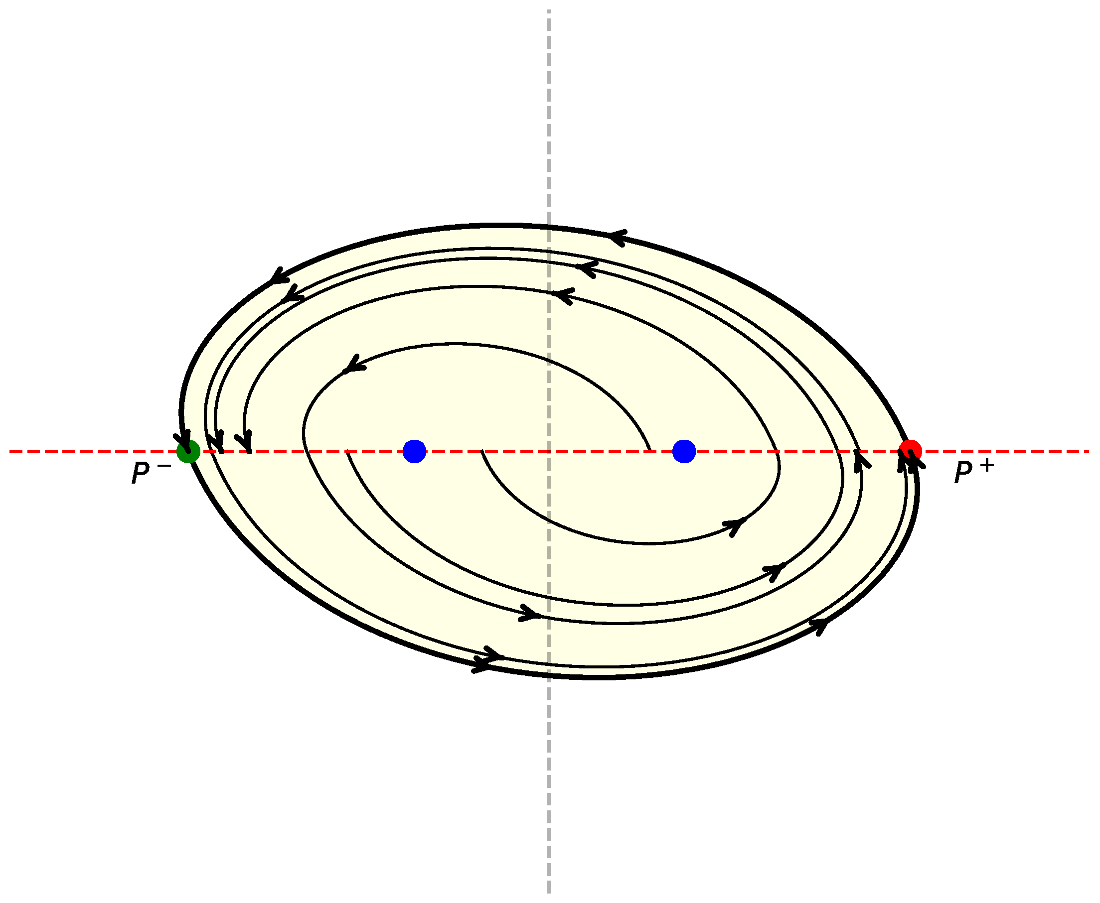
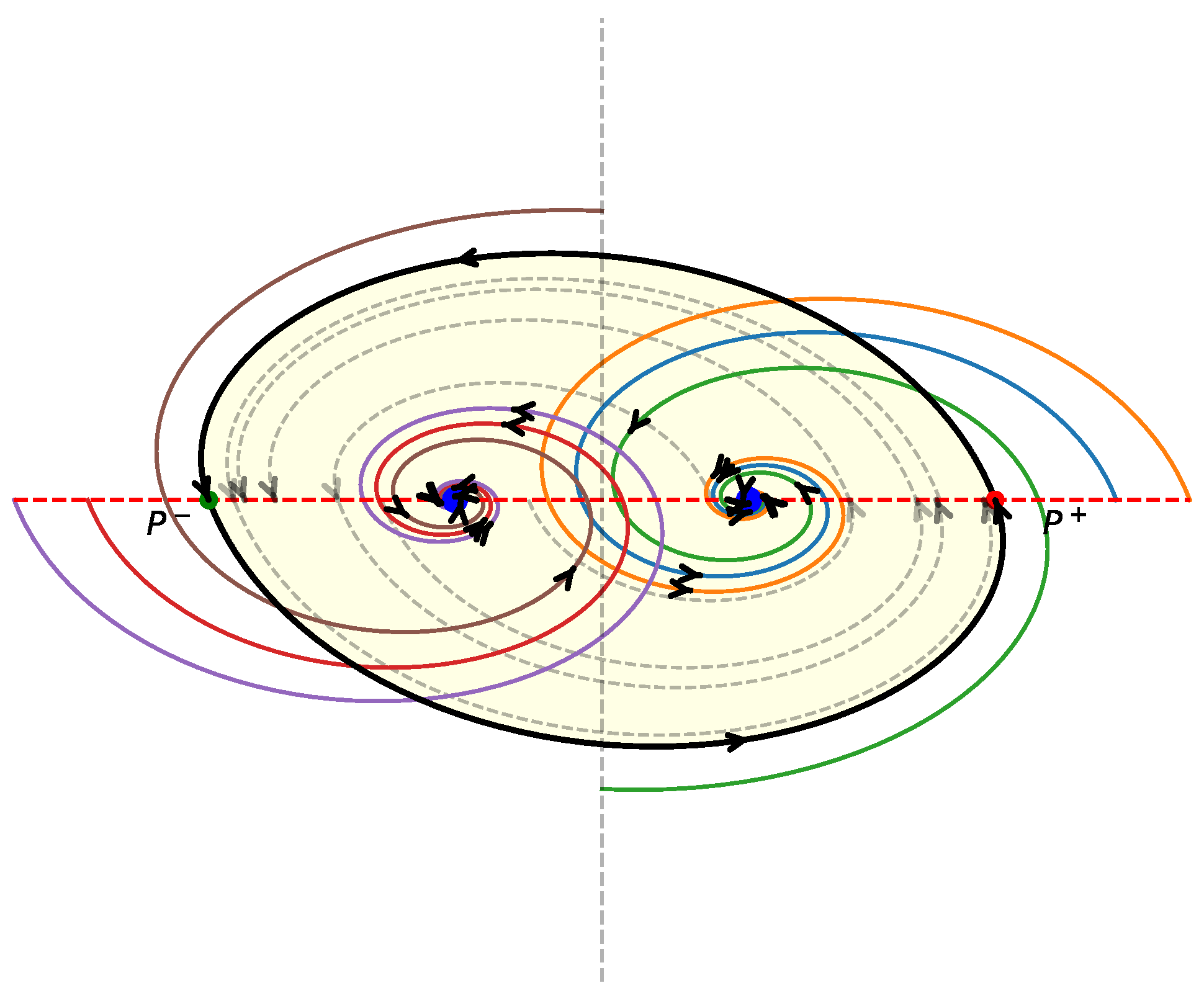
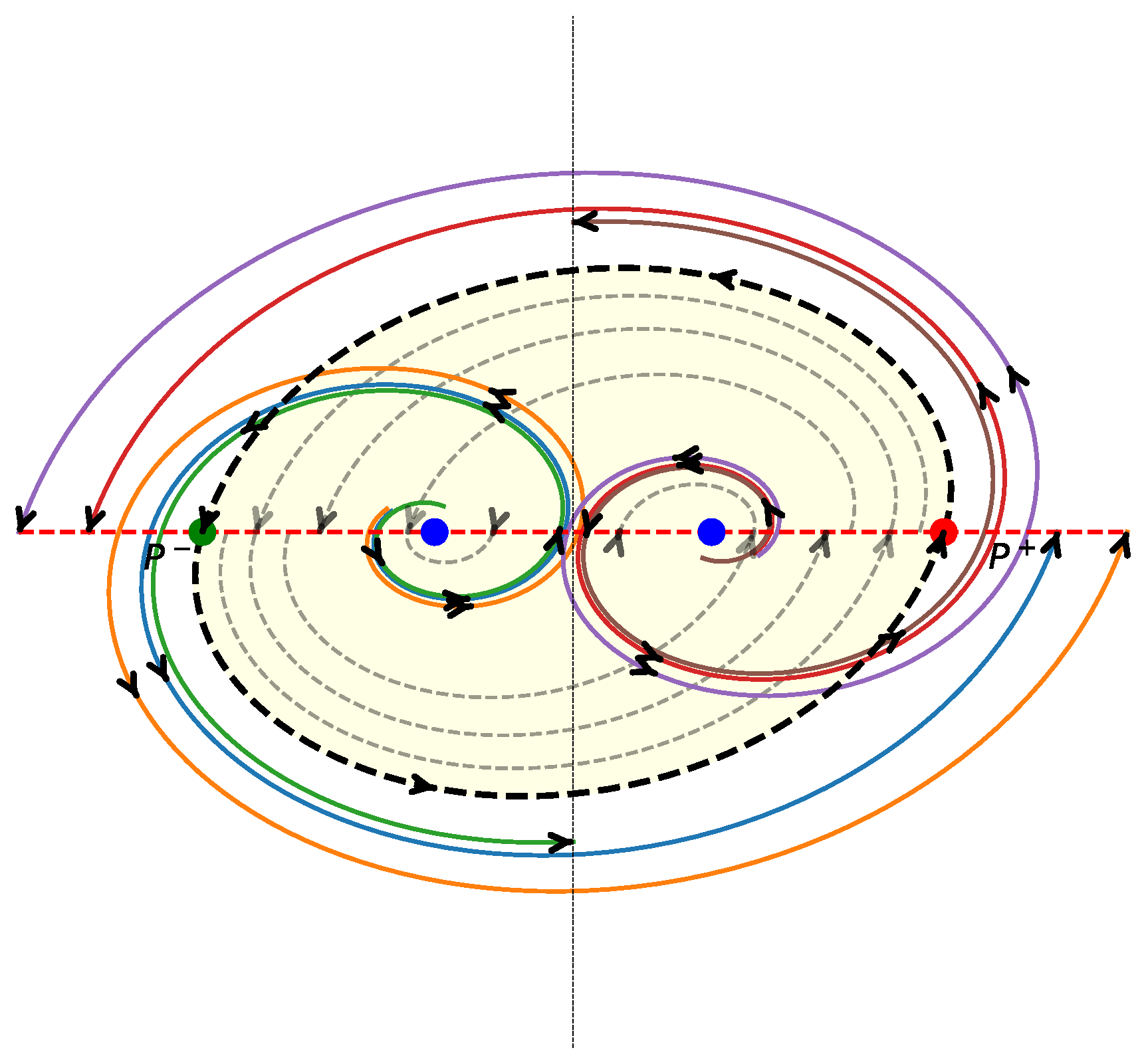
4.2.2. The Case $detA\ne 0$ and $trA\ne 0$

In this section, we show how to construct a periodic orbit for ${\mathsf{\Sigma }}_{{\mathbb{R}}^2}$, which is the boundary of the unique control set with non-empty interior.

Assume the eigenvalues of A are $\lambda \pm \mu i$ with $\lambda <0$ and $\mu >0$. Define recurrently

$$P_0=v\left(u^{+}\right),P_{2n+1}:=\phi \left({\displaystyle \frac{\pi }{\mu }},P_{2n},u^{-}\right)\mathrm{and}{P}_{2n+2}:=\phi \left({\displaystyle \frac{\pi }{\mu }},P_{2n+1},u^{+}\right),n\ge 0.$$

It is possible to prove that the odd and even sequences are convergent. Precisely,

$$P_{2n}\to P^{+}:=\left({\displaystyle \frac{-u^{+}+{\mathrm{e}}^{\pi \frac{\lambda }{\mu }}{u}^{-}}{1-{\mathrm{e}}^{\pi \frac{\lambda }{\mu }}}}\right)A^{-1}b\mathrm{and}{P}_{2n+1}\to P^{-}:=\left({\displaystyle \frac{-u^{-}+{\mathrm{e}}^{\pi \frac{\lambda }{\mu }}{u}^{+}}{1-{\mathrm{e}}^{\pi \frac{\lambda }{\mu }}}}\right)A^{-1}b.$$

Moreover, it turns out that the subset of ${\mathbb{R}}^2$ given by

$$\mathcal{O}:=\left\{\phi (t,P^{+},u^{-}),t\in \left[0,{\displaystyle \frac{\pi }{\mu }}\right]\right\}\cup \left\{\phi (t,P^{-},u^{+}),t\in \left[0,{\displaystyle \frac{\pi }{\mu }}\right]\right\},$$

is a periodic orbit of ${\mathsf{\Sigma }}_{{\mathbb{R}}^2}$. Let us denote by $\mathcal{C}$ the closure of the region delimited by $\mathcal{O}$.

With all this information, we are willing to establish the control sets in this context.

The main result concerning the control sets of this system reads as follows.

Theorem 8.

For the LCS ${\mathsf{\Sigma }}_{{\mathbb{R}}^2}$ with ${\sigma }_A<0$ and $trA\ne 0$ it holds

(a)

$trA<0$ implies that $\mathcal{C}$ is a control set

(b)

$trA>0$ infers that $int\mathcal{C}$ and $\mathcal{O}$ are the only control sets of ${\mathsf{\Sigma }}_{{\mathbb{R}}^2}$.

Figure 6. Periodic Orbit

Figure 6. Periodic Orbit

Figure 7. Case (a)

Figure 7. Case (a)

Figure 8. Case (b)

Figure 8. Case (b)

5. The LCSs on the 2-Dimensional Solvable Lie Group

Here, we follow the reference [3]. We analyze the control sets of a linear control system on the 2-dimensional connected affine group:

$$G={\mathrm{Aff}}_{+}\left(2\right)=\left\{\left(\begin{array}{cc}x& y\\ 0& 1\end{array}\right);(x,y)\in {\mathbb{R}}^{+}\times \mathbb{R}\right\}.$$

In order to simplify calculations, the authors in [3] introduce the G-automorphism: $\psi :G\to G$

$$\psi (x,y)=(x,c(x-1)+dy),d\in {\mathbb{R}}^{*}.$$

which preserves linear and left-invariant vector fields and hence conjugates linear control systems.

The underlying manifold of G is the open half-plane structure ${\mathbb{R}}^2$ endowed with the product

$$(x_1,y_1)·(x_2,y_2)=(x_1{x}_2,y_2+x_2{y}_1).$$

Its Lie algebra $\mathfrak{g}=\mathrm{aff}\left(2\right)$ is generated by the left-invariant vector fields $X=x{\displaystyle \frac{\partial }{\partial x}}$ and $Y=x{\displaystyle \frac{\partial }{\partial y}}$. Since $[X,Y]=Y$, $\mathfrak{g}$ is solvable and also G.

Under the basis $X,Y$, any derivation D of $\mathrm{aff}\left(2\right)$ reads as $D=\left(\begin{array}{cc}0& 0\\ a& b\end{array}\right),$ where a and b are real numbers.

The corresponding linear vector field $\mathcal{X}$ on G associated to D, has the form

$$\mathcal{X}(x,y)=(0,a(x-1)+by),\mathrm{with}(a,b)\in {\mathbb{R}}^2.$$

Moreover, any left-invariant vector field of G is depends on two parameters

$$Y(x,y)=(x\alpha ,x\beta ),\mathrm{for}\mathrm{some}(\alpha ,\beta )\in {\mathbb{R}}^2.$$

Definition 7.

A linear control system on G is a system of the form,

$$(\dot{x},\dot{y})=\mathcal{X}(x,y)+uY(x,y),withu\in \mathsf{\Omega }.$$

Here, $\mathcal{X}$ is linear and Y is left-invariant, where, $\mathsf{\Omega }=[u_{-},u^{+}]$ with $u_{-}<0<u^{+}$.

In coordinates, the system reads as follows

$$\begin{array}{cccc}& & \hfill \left\{\begin{array}{c}\dot{x}=u\alpha x\hfill \\ \dot{y}=a(x-1)+by+ux\beta \hfill \end{array}\right.,whereu\in \mathsf{\Omega }and(a,b),(\alpha ,\beta )\in {\mathbb{R}}^2\setminus \left\{(0,0)\right\}.\left({\mathsf{\Sigma }}_G\right)& \end{array}$$

It is straightforward to show that

$$\mathcal{L}(x,y)=\mathrm{span}\left\{\right(u\alpha x,a(x-1)+by+ux\beta ),(0,ux(a\alpha +b\beta )),u\in \mathsf{\Omega }\}.$$

And, the LARC holds for $\mathsf{\Sigma }$ if and only if $\alpha (a\alpha +b\beta )\ne 0$.

Remark 1.

Since the identity element e of G is a singularity of the drift and by hypothesis 0 belongs to the interior of omega, it turns out that there exists a control set $\mathcal{C}$ containing the identity. Moreover, e belongs to the interior of $\mathcal{C}$ if and only if ${\mathcal{O}}^{+}\left(e\right)$ is open. Again,

$$\mathcal{C}=cl\left({\mathcal{O}}^{+}\left(e\right)\right)\cap {\mathcal{O}}^{-}\left(e\right).$$

5.1. The Case $\alpha (a\alpha +b\beta )\ne 0$

In this section, we analyze the control sets of an LCS on $G={\mathrm{Aff}}_{+}\left(2\right)$ under the LARC. The existing control set is unique and has a non-empty interior. The analysis is according to the different possibilities of b.

It is worth to mention that in [8] the authors prove that $b=0$ and the LARC are equivalent to the controllability of a LCS. Here, we explicitly show the curves connecting any two arbitrary states.

5.1.1. The Case $b=0$

Under the hypothesis it follows that $a\ne 0$. Therefore, the diffeomorphism

$$\psi (x,y):=(x,a^{-1}y-\beta {\alpha }^{-1}(x-1)),$$

conjugates $\mathsf{\Sigma }$ and the new linear control system:

$$\left\{\begin{array}{c}\dot{x}=u\alpha x\hfill \\ \dot{y}=x-1\hfill \end{array}\right.,\mathrm{where}u\in \mathsf{\Omega }.$$

The solutions starting at $(x,y)\in G$ are given by the concatenations of the flows

$$\phi (t,(x,y),u)=\left({\mathrm{e}}^{u\alpha t}x,{\displaystyle \frac{({\mathrm{e}}^{u\alpha t}-1)x}{u\alpha }}-t+y\right),t\in \mathbb{R},u\ne 0$$

and,

$$\phi (t,(x,y),0)=\left(x,(x-1)t+y\right),t\in \mathbb{R},u=0.$$

Theorem 9.

If $b=0$ the system Σ is controllable in G.

Figure 9. $b=0$ the system $\mathsf{\Sigma }$ is controllable in G

Figure 9. $b=0$ the system $\mathsf{\Sigma }$ is controllable in G

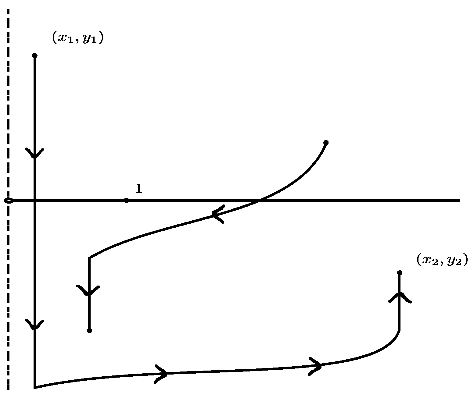
5.1.2. The Case $b\ne 0$

Assume $b<0$, the other case is analogous. Through the G-diffeomorphism defined by

$$\psi (x,y):=(x,{\gamma }^{-1}(a(x-1)+by)),$$

where $\gamma =a\alpha +b\beta \ne 0$, the system $\mathsf{\Sigma }$ is conjugated to the new LCS

$$\left\{\begin{array}{c}\dot{x}=u\alpha x\hfill \\ \dot{y}=by+ux\hfill \end{array}\right.,\mathrm{where}u\in \mathsf{\Omega }.$$

(2)

The integral curves starting at $(x,y)\in G$ of (2) are given by concatenations of the flows

$$\begin{array}{c}\phi (t,(x,y),u)=({\mathrm{e}}^{u\alpha t}x,m_u({\mathrm{e}}^{u\alpha t}-{\mathrm{e}}^{bt})x+{\mathrm{e}}^{bt}y),\mathrm{for}u\alpha \ne b\mathrm{and}{m}_u={\displaystyle \frac{u}{u\alpha -b}}\\ \\ \mathrm{and}\phi (t,(x,y),b{\alpha }^{-1})=\left({\mathrm{e}}^{bt}x,{\mathrm{e}}^{tb}(y+tb{\alpha }^{-1}x)\right),t\in \mathbb{R},\mathrm{when}u\alpha =b.\end{array}$$

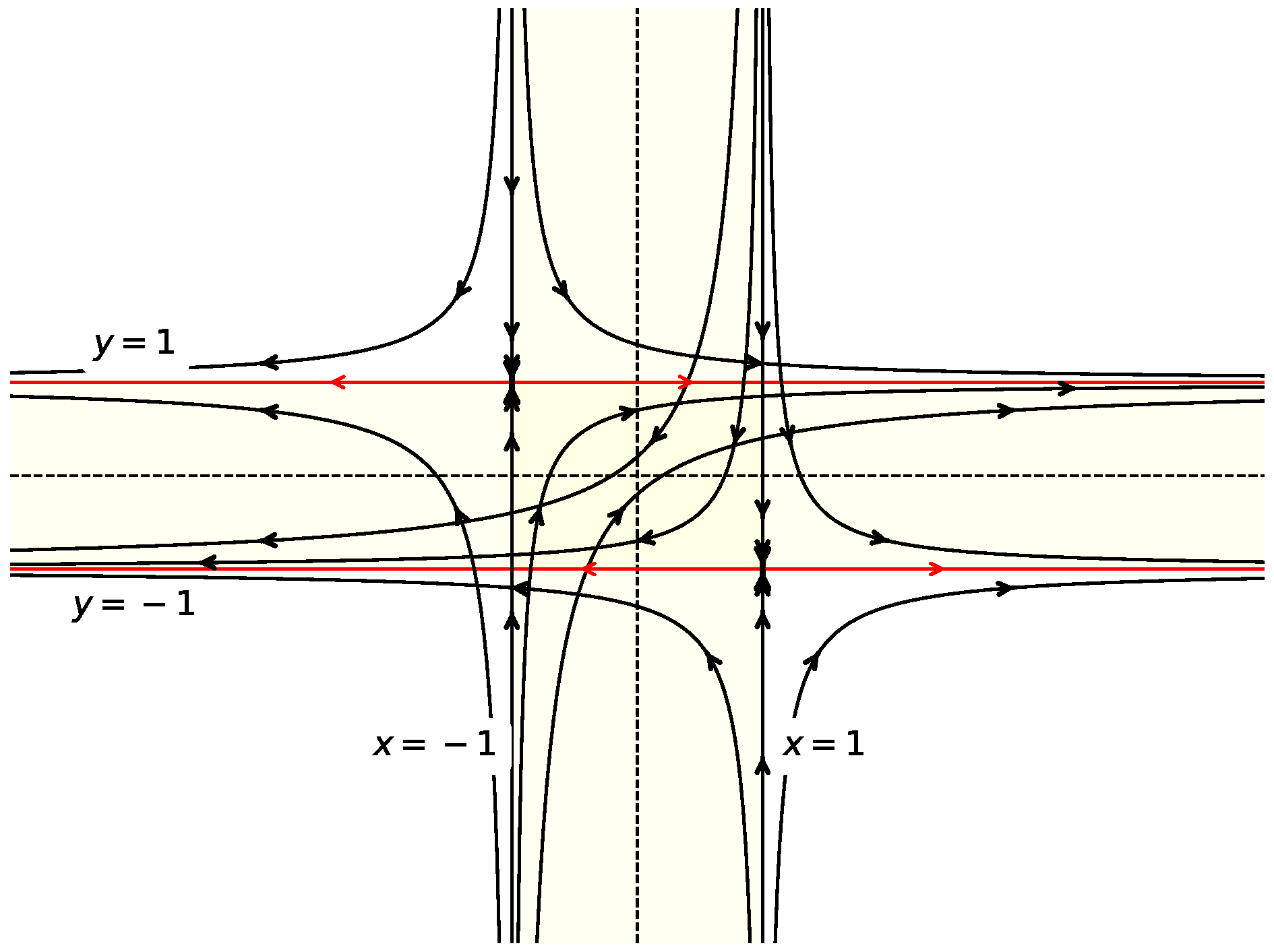
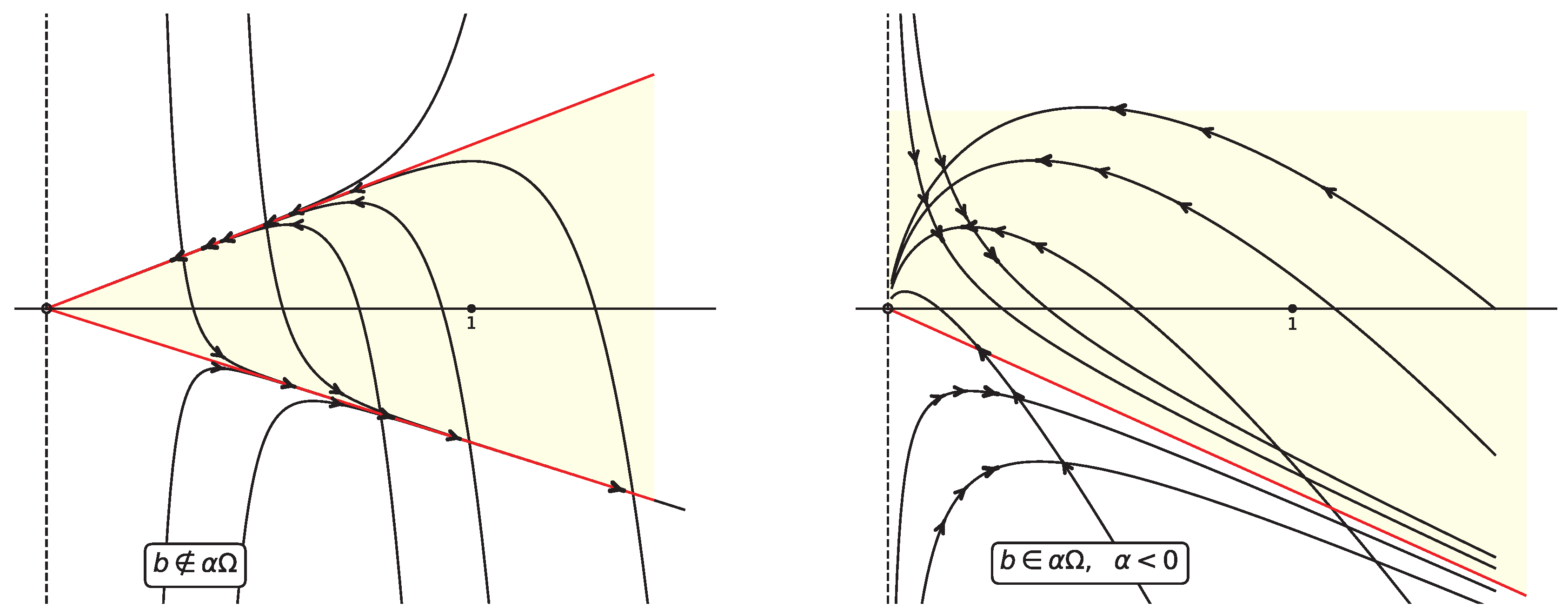
Next, we mention the main result of this section.

Theorem 10.

If $b<0$ the unique control set of (2) is $\mathcal{C}=cl\left({\mathcal{O}}^{+}(x,y)\right)$, for any $(x,y)\in \mathcal{C}$.

The following results describe all control sets of an LCS on the two-dimensional solvable Lie group. It also considers the case when the system does not satisfy the LARC.

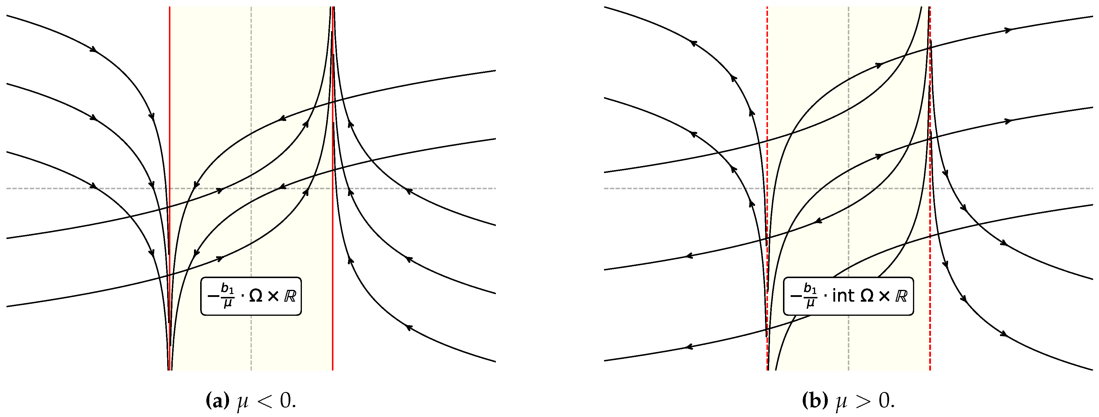
Theorem 11.

For the linear control system Σ it holds:

1.

$\alpha =a\alpha +b\beta =0$ and any vertical line close to $(1,0)$ is a control set;

2.

$\alpha =0$ and $a\alpha +b\beta \ne 0$, and the control sets are vertical segments intersecting

$$\{(x,y)\in G;y=-a{b}^{-1}(x-1)\};$$

3.

$\alpha \ne 0$ and $a\alpha +b\beta =0$, and Σ admits only the control set

$$\{(x,y)\in G;y=\beta {\alpha }^{-1}(x-1)\};$$

4.

$\alpha (a\alpha +b\beta )\ne 0$ with $b=0$ and the unique control set is the whole G;

5.

$\alpha (a\alpha +b\beta )\ne 0$ with $b\ne 0$ and the unique control set is a cone in G with (open) edge on the point $(0,a{b}^{-1})$.

Figure 10. Illustrative images of Theorem 10.

Figure 10. Illustrative images of Theorem 10.

Remark 2.

Let us notice that items 1. and 2. of Lemma 3.4 in [3] show that $\mathcal{C}$ is a cone in G with (open) wedge on $(0,0)\in {\mathbb{R}}^2$ (see Figure 9 below).

6. Examples Based on Control Sets

In what follows, we perform the control–set analysis for selected models on ${\mathbb{R}}^2$ and on the solvable group $G=Af{f}_{+}\left(2\right)$. In every case, we fix a bounded control range $\mathsf{\Omega }=[u^{-},u^{+}]$ with $u^{-}<0<u^{+}$ and emphasize: (i) the LARC (when used), and (ii) the explicit description of the control set(s) $\mathcal{C}$ given by the results in Section 4–5.

6.1. Planar Drivetrain with One Neutral Mode ($detA=0$, $trA\ne 0$)

A planar drivetrain with one neutral mode is a 2D mechanical control system whose dynamics include one zero-eigenvalue direction (persistent motion without decay) and one decaying direction. Control theory interprets it as a system that is stable in one direction and marginally stable (neutral) in another, requiring input to regulate the neutral degree of freedom [24]. Let

$$A=\left(\begin{array}{cc}-1& 0\\ 0& 0\end{array}\right),b=\left(\begin{array}{c}1\\ 1\end{array}\right),\mathsf{\Omega }=[-1,1].$$

In an eigenbasis of A this is the case $detA=0$, $trA=\mu =-1\ne 0$ of §4.2. LARC holds since $b_1{b}_2\ne 0$. By Theorem 4(a) with $\mu <0$,

$$\begin{array}{|c|}\hline {\mathcal{C}}_{{\mathbb{R}}^2}=\left(-\frac{b_1}{\mu }\mathsf{\Omega }\right)\times \mathbb{R}=\mathsf{\Omega }\times \mathbb{R}. \\ \hline\end{array}$$

Application meaning. The first coordinate (damped mode) is fully controllable within a bounded interval, while the neutral mode is transitively reachable along vertical fibers.

6.2. Planar Servo with Antagonist Damping (Real Eigenvalues, $detA<0$)

In a human elbow joint, the biceps flexes while the triceps extends. If both are slightly activated together, they produce antagonist damping that prevents the joint from trembling or overshooting. Or in a robotic planar arm with two opposing motors: One motor pushes forward, the other resists in the opposite direction. The control system introduces a velocity-proportional opposing force, effectively creating a virtual damper. This situation can be modeled through the classical LCS on ${\mathbb{R}}^2$, [33]

$$\dot{v}=Av+ub,u\in \mathsf{\Omega }=[-1,1],A=\left(\begin{array}{cc}1& 0\\ 0& -1\end{array}\right),b=\left(\begin{array}{c}1\\ 1\end{array}\right).$$

Since b is not an eigenvector of A, LARC holds. This is the diagonal case with $\lambda <0<\mu$ (§4.3). By Theorem 5 the system has a unique control set with nonempty interior,

$$\begin{array}{|c|}\hline {\mathcal{C}}_{{\mathbb{R}}^2}=(-1,1)\times [-1,1]\\ \hline\end{array}.$$

Application meaning. The rectangle describes the maximal region in which any two admissible states (angle/velocity offsets) can be mutually reached using bounded torques.

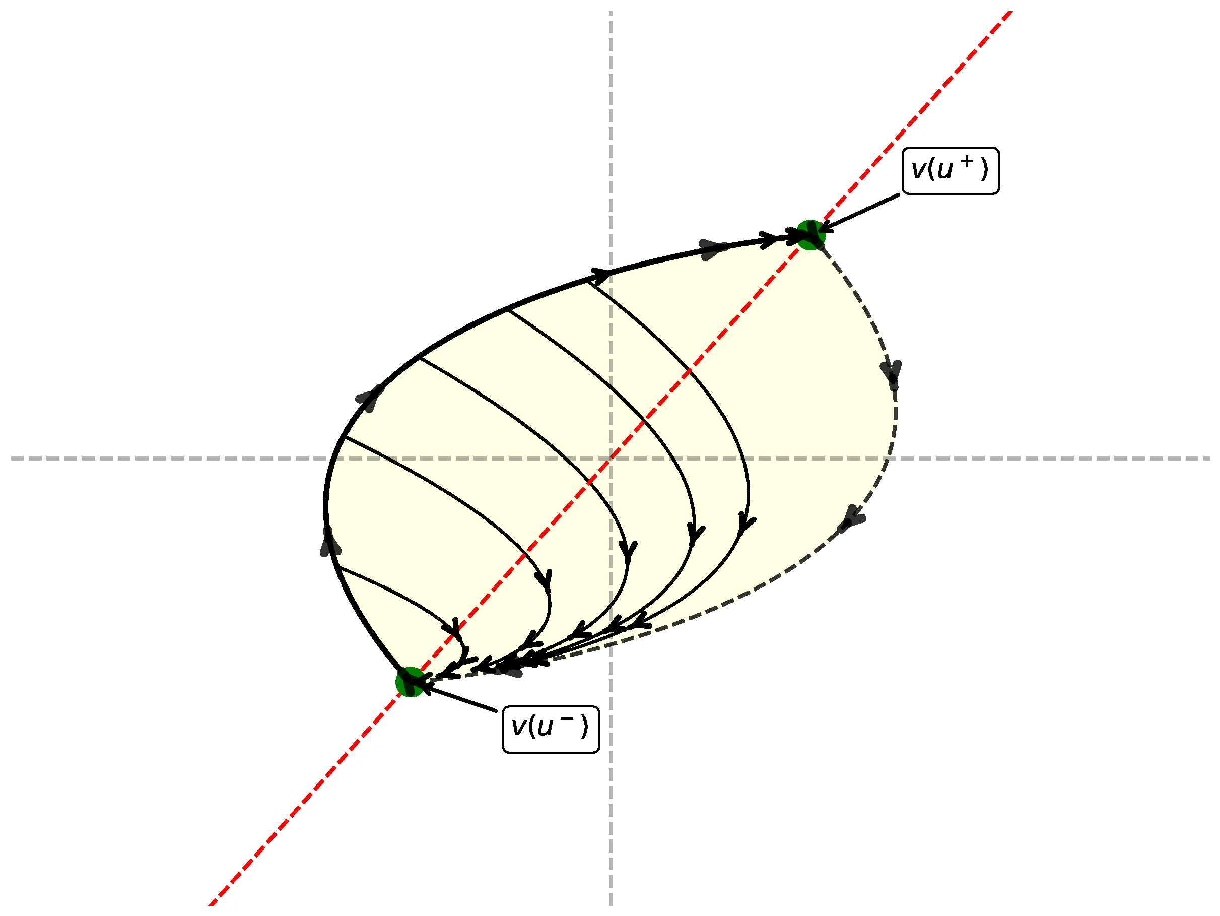
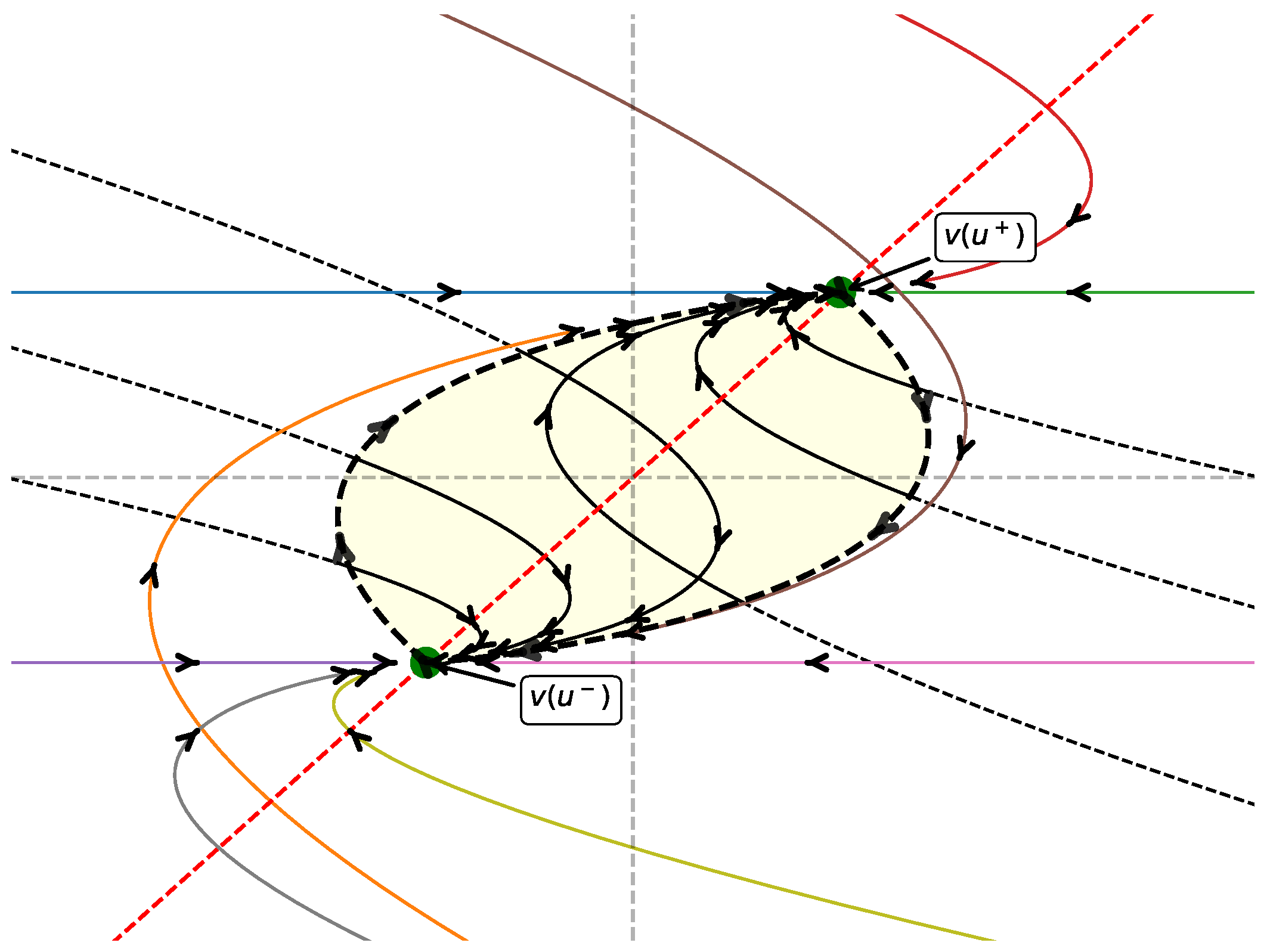
6.3. Planar Oscillator with Complex Eigenvalues and Decay ($trA<0$)

Think of a mass on a spring with a dashpot (damper). Now forget the usual “position vs. time” plot and instead watch the system in a plane whose axes are: horizontal axis = position and vertical axes the velocity. Therefore, (x,v) in this state (phase) plane tells you exactly how the system is moving right now. As time flows, the point traces a curve—its trajectory—showing how position and velocity co-evolve, [11] Let

$$A=\left(\begin{array}{cc}-1& -2\\ 2& -1\end{array}\right),b=\left(\begin{array}{c}1\\ 0\end{array}\right),\mathsf{\Omega }=[-1,1],$$

so that ${\sigma }_A={(trA)}^2-4detA<0$ and $trA<0$ (§4.4). As in Theorem 8, the system admits a unique control set $\mathcal{C}$ whose boundary is a periodic orbit built by alternating the constant controls $u^{\pm }=\pm 1$ over half–periods $\pi /\mu$ (here $\mu =2$):

$$\mathcal{O}=\left\{\phi (t,P^{+},u^{-}):0\le t\le \frac{\pi }{2}\right\}\cup \left\{\phi (t,P^{-},u^{+}):0\le t\le \frac{\pi }{2}\right\},$$

with

$$P^{\pm }=\left({\displaystyle \frac{-u^{\pm }+e^{\pi \frac{trA}{\mu }}{u}^{\mp }}{1-e^{\pi \frac{trA}{\mu }}}}\right)A^{-1}b=\pm {\displaystyle \frac{1+e^{-\pi /2}}{1-e^{-\pi /2}}}{A}^{-1}b,A^{-1}b={\displaystyle \frac{1}{5}}\left(\begin{array}{c}-1\\ -2\end{array}\right).$$

Then $\mathcal{C}$ is the closed region enclosed by $\mathcal{O}$ (nonempty interior).

$$\begin{array}{|c|}\hline int\mathcal{C}\ne \varnothing ,\partial \mathcal{C}=\mathcal{O}\\ \hline\end{array}.$$

Application meaning. In a lightly damped planar mode with bounded actuation (e.g., piezo stage with saturation), the periodic boundary provides a constructive protocol to scan the boundary of the maximal controllable domain, [26].

6.4. Linear Control on $Af{f}_{+}\left(2\right)$ with $b=0$ (Global Controllability)

On $G=Af{f}_{+}\left(2\right)$ in coordinates $(x,y)$ consider

$$\dot{x}=u\alpha x,\dot{y}=a(x-1)+by+ux\beta ,\mathsf{\Omega }=[-1,1],$$

with parameters $a=1,b=0,\alpha =1,\beta =0$. Then $a\alpha +b\beta =1\ne 0$ and $\alpha \ne 0$, hence LARC holds. By Theorem 5.2 (case $b=0$),

$$\begin{array}{|c|}\hline {\mathcal{C}}_G=G(\mathrm{the}\mathrm{whole}\mathrm{group})\\ \hline\end{array}.$$

By analyzing the system dynamics under specific parameter conditions, the entire group is reachable from any initial state, establishing complete controllability. The theoretical results can be illustrated through concrete examples, highlighting the practical implications for systems requiring precise maneuvering. These findings have broad relevance in robotics, automation, and control engineering, where ensuring system flexibility and maneuverability is critical for operational success.

6.5. Neuroscience Application: Control Sets for Orientation Dynamics in $V1$

A simplified model of cortical responses in the primary visual cortex $V1$ can be framed as an LCS on the solvable Lie group $G=Af{f}_{+}\left(2\right)$, where states $(x,y)\in {\mathbb{R}}^{+}\times \mathbb{R}$ encode, respectively, (i) an orientation selectivity/gain-like variable ($x>0$) and (ii) a response bias/excitability coordinate (y). External visual drive and local circuitry are modeled as a bounded scalar control $u\in \mathsf{\Omega }=[-1,1]$ acting through a left-invariant field. With the linear field $\mathcal{X}$ associated to a derivation D and a left-invariant field Y, the system reads

$$(\dot{x},\dot{y})=\mathcal{X}(x,y)+uY(x,y),\mathcal{X}(x,y)=(0,a(x-1)+by),Y(x,y)=(\alpha x,\beta x).$$

Hence,

$$\dot{x}=u\alpha x,\dot{y}=a(x-1)+by+u\beta x,u\in [-1,1],$$

(3)

with parameters $a,b,\alpha ,\beta \in \mathbb{R}$.

Control–set regimes and cortical interpretation. We summarize the geometry of control sets $\mathcal{C}$ for (3) and its direct meaning for $V1$ dynamics; all statements refer to the results in Section 5.

Homogeneous propagation (no decay): $b=0$. If $a\ne 0$ and $\alpha \ne 0$, the LARC holds and by Theorem 5.2 the system is globally controllable, i.e.

$$\begin{array}{|c|}\hline \mathcal{C}=G\\ \hline\end{array}.$$

V1 meaning: orientation preference/gain can be steered between any two states with bounded input; there are no excluded cortical response regions.

Constrained propagation (decay): $b<0$. Assume $\alpha \ne 0$ and $a\alpha +b\beta \ne 0$ (LARC). By Theorem 10 and the classification of Theorem 5.5, there is a unique control set with nonempty interior, which is a cone in G with (open) edge at $(0,a/b)$:

$$\begin{array}{|c|}\hline \mathcal{C}=cl\left({\mathcal{O}}^{+}(x_0,y_0)\right)(\mathrm{any}(x_0,y_0)\in \mathcal{C})\\ \hline\end{array}.$$

V1 meaning: only a conic domain of orientation–gain states is mutually reachable; “blind zones’’ appear outside the cone.

Degenerate modulation: $\alpha =0$, $a\alpha +b\beta \ne 0$. By Theorem 5.5 the control sets collapse to vertical segments intersecting the line $\{y=-a{b}^{-1}(x-1)\}$:

$$\begin{array}{|c|}\hline \mathcal{C}=\mathrm{vertical}\mathrm{segments}\mathrm{in}x>0\mathrm{along}\mathrm{invariant}\mathrm{fibers}\\ \hline\end{array}.$$

V1 meaning: orientation selectivity cannot be changed by inputs; dynamics are confined to 1D fibers (response-bias modulation only).

Explicit envelope of the conic control set (case (C)).

Choose concrete parameters

$$a=1,b=-1,\alpha =1,\beta =0,\mathsf{\Omega }=[-1,1].$$

Then (3) becomes

$$\dot{x}=ux,\dot{y}=(x-1)-y,u\in [-1,1],$$

which satisfies LARC and $b<0$. For any constant control $u\ne -1$,

$$x\left(t\right)=e^{ut}{x}_0,y\left(t\right)={\displaystyle \frac{u}{u+1}}\left(e^{ut}-e^{-t}\right)x_0+e^{-t}{y}_0,$$

and for $u=-1$,

$$x\left(t\right)=e^{-t}{x}_0,y\left(t\right)=e^{-t}\left(y_0-t{x}_0\right).$$

Launching from $(x_0,y_0)=(1,0)$ and eliminating t yields the envelope curves generated by extreme controls:

$$y_u\left(x\right)={\displaystyle \frac{u}{u+1}}\left(x-x^{-1/u}\right),u\in (-1,1],y_{-1}\left(x\right)=xlnx.$$

Therefore, the control set is precisely the conic domain

$$\begin{array}{|c|}\hline \mathcal{C}=\left\{(x,y):x>0,y_{-1}\left(x\right)\le y\le y_1\left(x\right)=\frac{1}{2}(x-x^{-1})\right\}\cup \left\{\mathrm{orbits}\mathrm{connecting}\mathrm{the}\mathrm{envelopes}\right\}.\\ \hline\end{array}$$

V1 meaning: stimuli and intracortical inputs can steer responses only within the cone bounded by $y=xlnx$ and $y=\frac{1}{2}(x-x^{-1})$; outside this region, states are not mutually reachable by admissible controls—mathematically capturing “restricted propagation’’ of orientation activity.

7. Conclusions with Future Work

In the context of Lie groups, the dynamical behavior of LCSs has been extensively studied by our team utilizing the inherent geometric richness found within Lie theory. The class of LCS on G poses a significant challenge due to the complexity of the state space and the dynamics involved. According to the Levy theorem [18], any Lie algebra can be decomposed into a solvable and a semisimple part. Highlighting the importance of considering these cases separately.

Since 2017, our team has been focused on studying controllability, control sets, observability, and optimal problems for this class of systems on different classes of Lie groups, nilpotent, solvable, and semisimple [2,3,6,7,8,10]. Thus, our future research will include to investigate for algebraic, topological, geometrical, and dynamical properties that characterize stability for a linear control system (LCS), on an arbitrary connected Lie group in various scenarios: Abelian, nilpotent, solvable, semisimple, and arbitrary groups through the Lévy Theorem, and their homogeneous spaces.

References

- Agrachev, A.; Barilari, D.; Boscain, U. A comprehensive introduction to sub-Riemannian geometry; Cambridge University Press, 2019; Vol. 181. [Google Scholar]
- Ayala, V.; Tirao, J. Linear control systems on Lie groups and Controllability.; American Mathematical Society. Series: Symposia in Pure Mathematics, Vol. 64, n∘1; 1999; pp. 47–64. [Google Scholar]
- Ayala, V.; Da Silva, A. The control set of a linear control system on the two-dimensional Lie group. Journal of Differential Equations 2020, 268, 6683–6701. [Google Scholar]
- Ayala, V.; Da Silva, A.; Rojas, A.F. Control sets of linear control systems on R2. The real case. Nonlinear Differential Equations and Applications NoDEA 2024, 31(5), 94. [Google Scholar] [CrossRef]
- Ayala, V.; Da Silva, A.; Mamani, E. Control sets of linear control systems on . The complex case. ESAIM- Control, Optimization and Calculus of Variations 2023, 29, 1–16. [Google Scholar] [CrossRef]
- Ayala, V.; Da Silva, A. On the characterization of the controllability property for linear control systems on non-nilpotent, solvable three-dimensional Lie groups. Journal of Differential Equations 2019, 266, 8233–8257. [Google Scholar] [CrossRef]
- Ayala, V.; Da Silva, A. Controllability of linear control systems on Lie groups with semisimple finite center. SIAM Journal on Control and Optimization 2017, 55, 1332–1343. [Google Scholar] [CrossRef]
- Ayala, V.; Da Silva, A. Linear control systems on the homogeneous spaces of the 2D Lie group. Journal of Differential Equations 2022, 314, 850–870. [Google Scholar] [CrossRef]
- Ayala, V.; Da Silva, A.; Zsigmond, G. Control sets of linear systems on Lie groups. Nonlinear Differential Equations and Applications - NoDEA 2017, 24, 1–15. [Google Scholar] [CrossRef]
- Ayala, V.; Da Silva, A.; Zsigmond, G. Control sets of linear systems on semisimple Lie groups. Journal of Differential Equations 2020, 269, 449–466. [Google Scholar] [CrossRef]
- Bechhoefer, J. Feedback for physicists: A tutorial essay on control. Reviews of Modern Physics 2005, 77, 783–836. [Google Scholar] [CrossRef]
- Brockett, R. W. System theory on group manifolds and coset spaces. SIAM Journal on control 1972, 10, 265–284. [Google Scholar] [CrossRef]
- Bullo, F.; Lewis, A.D. Geometric control of mechanical systems: modeling, analysis, and design for simple mechanical control systems. Springer, 2019; Vol. 49. [Google Scholar]
- Colonius, F.; Kliemann, C. The Dynamics of Control; Systems and Control: Foundations and Applications; Birkhäuser Boston, Inc., 2000. [Google Scholar]
- Da Silva, A.; Rojas, A.F. Weak condition for the existence of control sets with a non-empty interior for linear control systems on nilpotent groups. Mathematics of Control, Signals, and Systems 2024, 1–19. [Google Scholar]
- Da Silva, A. Controllability of linear systems on solvable Lie groups. SIAM Journal on Control and Optimization 2016, 54, 372–390. [Google Scholar] [CrossRef]
- Dath, M.; Jouan, P. Controllability of linear systems on low dimensional nilpotent and solvable Lie groups. Journal of Dynamical and Control Systems 2016, 22, 207–225. [Google Scholar] [CrossRef]
- Helgason, S. Differential Geometry, Lie Groups, and Symmetric Spaces; Academic Press, 1978. [Google Scholar]
- Jean, F. Control of nonholonomic systems: from sub-Riemannian geometry to motion planning; Springer, 2014. [Google Scholar]
- Jouan, Ph. Equivalence of control systems with linear systems on Lie groups and homogeneous spaces. ESAIM: Control Optimization and Calculus of Variations 2010, 16, 956–973. [Google Scholar] [CrossRef]
- Jouan, Ph. Controllability of linear systems on Lie group. J. Dyn. Control Syst. 2011, 17, 591–616. [Google Scholar] [CrossRef]
- Jurdjevic, V. Geometric Control Theory. Cambridge Studies in Advanced Mathematics 1997, 52. [Google Scholar]
- Leitmann, G. OptimizationTechniques with Application to Aerospace Systems; Academic Press Inc.: London, 1962. [Google Scholar]
- Leonard, N.E.; Marsden, J.E. Stability and Control of Mechanical Systems with Zero Eigenvalues. IEEE Transactions on Automatic Control 1997, 42(1), 32–45. [Google Scholar]
- Markus, L. Controllability of multi-trajectories on Lie groups. In Proceedings of Dynamical Systems and Turbulence, Warwick; Lecture Notes in Mathematics 898; 1980; pp. 250–265. [Google Scholar]
- Morse, A.S.; Shiriaev, A. -of-attraction control of nonlinear systems: A geometric approach. IEEE Transactions on Automatic Control IEEE Transactions on Automatic Control, 60(4), 1018-1024. 2015, 60, 1018–1024. [Google Scholar]
- Sachkov, Y. L. Controllability of invariant systems on Lie groups and homogeneous spaces. Journal of Mathematical Sciences 2000, 100, 2355–2427. [Google Scholar] [CrossRef]
- San Martin, L. A. B. Invariant control sets on flag manifolds. Mathematical Control, Signals, and Systems 1993, 6, 41–61. [Google Scholar] [CrossRef]
- San Martin, L. A. B. Algebras de Lie, 2nd ed.; Editora Unicamp, 2010. [Google Scholar]
- Schättler, H.; Ledzewicz, U. Geometric Optimal Control. Theory, Methods and Examples; Interdisciplinary Applied Mathematics; Springer: New York, 2012; Vol. 38. [Google Scholar]
- Shell, K. Applications of Pontryagin’s Maximum Principle to Economics; Mathematical Systems Theory and Economics I and II, Volume 11/12 of the series Lecture Notes in Operations Research and Mathematical Economics, 241-292; 1968. [Google Scholar]
- Sontag, E.D. Mathematical control theory: deterministic finite dimensional systems; Springer Science and Business Media, 2013; Vol. 6. [Google Scholar]
- Spong, W.; Hutchinson, S.; Vidyasagar, M. Robot Modeling and Control; Wiley www.wiley.com, December 2005; 20 December 2006. [Google Scholar]
- Wonham, M.W. Linear Multivariable Control: A Geometric Approach, Applications of Mathematics; Springer: New York, NY, USA, 1979; Volume 10, p. 326. [Google Scholar]