Submitted:
02 September 2025
Posted:
03 September 2025
You are already at the latest version
Abstract
Partial discharges (PDs) are critical phenomena in diagnosing the insulation condition of electrical equipment using dielectric oils. Their early detection and characterization are fundamental for the prevention of catastrophic failures. This work presents an innovative bimodal approach for laboratory PD analysis through the training of a convolutional neural network (CNN) based on YOLOv8. Firstly, a conventional DDX-type PD electrical detector is enhanced by endowing it with smart capabilities. Through the CNN training, a system is then developed capable of automatically reading and interpreting data dis-played on an electrical detector screen, such as discharge magnitude, pulse count, and applied voltage. This transforms a conventional instrument into an autonomous source of digitized and structured data. The mean precision in the training was 0.91. Concurrently, an optical visualization system using a high-resolution camera is employed to capture direct images of PDs occurring in the dielectric oil. These images provide complementary qualitative and quantitative information, enabling the classification of discharge types based on their visual characteristics. For electrical voltages of 10, 13 and 16 kV, PDs were detected with confidence scores of up to 0.92. This study therefore combines quantitative information intelligently extracted from an electrical detector, with qualitative and mor-phological characterization obtained through optical analysis.
Keywords:
partial discharges
; dielectric oil
; electrical sensor
; optical sensor
; fault diagnosis
; predictive maintenance
; artificial intelligence
; YOLOv8
1. Introduction
Power transformers are fundamental components of a high-voltage electrical network, the failure of which can cause costly interruptions and long periods of downtime [1]. Dielectric oil, also known as transformer oil, is a high-purity, low-viscosity mineral oil which is essential for the operation of transformers and other electrical equipment. It serves a dual purpose, acting firstly as an electrical insulator between conductive components and secondly as a coolant, dissipating the heat generated by the core and windings. Bubbles within mineral oil are one of the most common defects in oil-paper insulation systems, weakening their structure and jeopardizing the operational safety of transformers [2]. This weakening is a precursor to the partial discharges (PDs) that can occur in them. The detection of PDs is a key aspect for preventive maintenance that helps to avoid transformer failure and for optimization of the number of scheduled transformer shutdowns.
PDs are important phenomena and one of the main indicators of the degradation of the integrity of electrical insulation, whether solid, liquid, or gaseous. They manifest as very short-duration electrical events —from tens of nanoseconds to microseconds— which the IEC 60270 [3] standard defines as localized, low-magnitude dielectric breakdowns. Although they do not cause immediate failure, their persistence over time can erode the insulation until it completely breaks down. Therefore, their early detection and accurate characterization are crucial to prevent catastrophic failures in high-voltage equipment.
Unimodal techniques (UTs) for PD detection are based on the diverse physical phenomena that accompany them. Each discharge, stochastic and aperiodic in nature, produces a current pulse. This pulse can produce acoustic waves, generate electromagnetic radiation, and release electrical charges [4]. The electrical method, standardized by IEC 60270 [3], is the reference technique for measurements in controlled laboratory environments due to its high sensitivity [5]. For monitoring under real-life operating conditions, non-conventional methods such as ultra-high frequency [6] and acoustic emission detection [7] are used. However, these techniques also present challenges such as the sensitivity of the acoustic method to the sensor location or the effects of radio frequency interference on the ultra-high frequency method [4].
It is well known that the patterns or signatures of PDs depend on the type of PD produced [8]. However, these patterns often require expert interpretation, which introduces subjectivity, limits scalability, and makes it difficult to accurately differentiate between different types of failures. This dependence on human factors constitutes a bottleneck for large-scale, real-time monitoring.
To overcome these limitations, the scientific community has turned to the use of artificial intelligence (AI), which has demonstrated superior ability to automate feature extraction, recognize complex patterns in data, and classify discharge types with accuracy, surpassing conventional methods [9] and opening a new era in isolation status diagnosis.
Despite advances in AI using UTs, the information derived from this detection method remains one-dimensional, whether electrical, acoustic, or electromagnetic in nature. AI analysis can optimize the interpretation of such data, but cannot generate more information.
Multisensory data fusion, or multimodal techniques (MTs), has emerged as a key strategy for overcoming the limitations of UT systems, representing one of the most promising frontiers in PD diagnosis. Comprehensive reviews of the state of the art, such as those presented in [10,11], provide in-depth analysis of the fundamentals, methodologies, benefits, and challenges of this discipline, demonstrating its potential for achieving more robust and reliable diagnoses.
In [12], a novel analysis method was developed that combines multimodal data and time sequences to provide rapid diagnosis in power transformers. In [13], an innovative bimodal transformer-based deep learning model was developed that uses optical data for PD classification. The system identifies sparks, corona, and surface discharges instantaneously, demonstrating near-perfect efficiency.
To improve the low accuracy of traditional PD recognition methods, in [14] a new system based on data fusion was presented. This method combines a statistical model and a CNN to analyze phase-resolved PD [15] images. The results of both are integrated using the Dempster-Shafer theory [16,17] achieving a recognition accuracy greater than 94%, which is a significant improvement over conventional approaches.
A robust diagnosis requires the synergy of two or more types of information. The present study integrates the information provided by an electrical sensor and an optical sensor. It combines the quantification of electrical severity by assessing the magnitude of the charge and the characterization of its location and physical morphology through optical imaging. Since no single method covers both dimensions, the combination of modalities is presented as an indispensable strategy for a complete understanding of the phenomenon.
Along these lines, our work proposes a bimodal approach that creates a unique synergy by combining the precise quantification of the electrical method with the spatial and morphological characterization of the optical method. Thus, while the electrical detector answers the question of the severity of the discharge magnitude, the optical detection analyzes the nature of the defect by locating its origin and shape. In both cases, AI analysis automates and enhances these two complementary procedures.
In PD detection in dielectric oils, the identification of the pulses produced is of great importance. All our tests are video recorded in order to extract as much information as possible. In this way, we detect and identify these pulses in real time. To carry out this task, YOLO (You Only Look Once) [18] is used as a tool for object detection in an image. We evaluated the use of YOLO because it can be used in Python environments with OpenCV [19].
YOLO models object detection as an extension of a regression problem, dividing the image into a series of cells and predicting bounding boxes and their confidence levels for each cell. This allows for a parallel search within the entire image, making it extremely fast when using graphics processing units (GPUs) at the same time.
Object detection is a core technology in many AI applications and is the fundamental goal of computer vision. In addition to detecting the presence of objects in images, it is also desirable to determine their position within them with an acceptable level of precision, as well as a confidence score of the class to which they belong.
It is a supervised learning problem that involves providing labeled data to an algorithm for training. Subsequently, when new unlabeled data unknown to the algorithm is introduced, it will be able to recognize certain patterns in the new data.
Presented by its authors in 2015 [18], YOLO is a set of open-source algorithms for real-time object detection. Its architecture introduces a paradigm shift and marks a milestone in the study of computer vision. It is a single-pass object detector that uses a complex CNN to predict bounding boxes and class probabilities for objects of interest in input images.
Previously, the most widely used approach to analyze images was the use of CNN and the sliding window concept. This involves choosing a window of a certain size and scanning the entire image, thereby detecting any trace of an object within that window. This method is very slow because it has to scan the entire image to try to find objects whose sizes, spatial orientations, and shapes can vary greatly. In contrast, YOLO can process images in real time with acceptable average accuracy at a speed of 155 frames per second (FPS).
Early versions of YOLO used a CNN architecture with a total of 24 convolutional layers, 4 max-pooling layers, and 2 fully connected layers. To operate, YOLO resizes the image by normalizing the input to 224, 448, or 640 pixels before passing it through the CNN.
Since the launch of its first version (YOLOv1), YOLO has evolved. Version v2 was launched in 2016 [20] and v3 in 2018 [21], with the introduction of the Darknet-19 architectures in v2 and Darknet-53 in v3. Versions v4 [22] and v5 [23] were launched in 2020, v6 [24] and v7 [25] in 2022, and v8 in 2023 [26].
This evolution has focused on increasing the detection speed by optimizing hyperparameters through the application of genetic algorithms. A comprehensive review of YOLO architectures in computer vision from YOLOv1 to YOLOv8 can be found in [27]. At the time of writing, the most recent released version is YOLOv12. For our work, we chose YOLOv8 because it is a mature technology and fits our real-time video processing needs, facilitating the use of GPUs to increase training and inference speeds.
YOLO has played a prominent role in numerous activities including, among others, applications in agriculture [28], industry [29], and the detection of objects in flight [30].
To implement this bimodal approach, two methods are combined. This article presents a novel diagnostic system for PD analysis in dielectric oils that integrates data from a conventional DDX electrical detector with high-speed image characterization using a YOLOv8 CNN [29]. The objective is to demonstrate that this combination of methods provides a substantially more complete and robust diagnostic view than that obtained separately, laying the foundation for more reliable and intelligent monitoring.
Based on this principle, our work presents a novel bimodal diagnostic system that combines electrical quantification using a DDX detector with optical characterization using a high quality camera (HQC). The main contribution lies in the synergistic fusion of these two electrical and optical sensors and the comprehensive automation of data interpretation using a GPU.
One of the key contributions of this study is the automation of both data sources. For the electrical sensor, a YOLOv8 model is developed that interprets and digitizes the DDX screen, transforming a conventional instrument into an intelligent data source. In parallel, for the optical sensor, a novel semi-automated methodology is presented for the generation of a high-quality dataset, which is a fundamental step for training. In both cases, intelligent inference of electrical and optical data is produced.
2. Experimental Set Up
In the present work, the PDs were measured in a dielectric oil located inside a methacrylate cell [31] containing two facing electrodes subjected to high electrical voltages (Figure 1). The experimental installation complies with the IEC60270 standard [3].
All tests lasted 45 s and were carried out at an ambient temperature of 21 °C. The PDs were monitored using a conventional DDX-9101 PD detector, and the high voltage was regulated using an OT 248 terminal (Figure 2).
The DDX-9101 screen was recorded by a digital camera to store the results of each test. This camera records video in 1920x1080p at 30 FPS.
Preliminary tests showed that PDs were practically non-existent below 6 kV and that electric arc breakdowns occurred from 18 kV onwards.
Taking this information into account, the PD were analyzed in a first series ranging from 6 to 18 kV. The voltage was increased by 1 kV in each test, thus performing 13 independent tests. The total duration of each experimental test was 45 s. The voltage applied to the electrodes started from 0 kV and followed an ascending ramp lasting approximately 10 s until reaching the desired nominal charge. After 45 s of testing, the electrical voltage was reduced to zero. A total of four sets of tests were performed from 6 to 18 kV. Therefore, the number of tests performed in this first series is 52.
These tests showed that PDs increase significantly above 10 kV. Therefore, it was decided to conduct a second series for voltages of 10, 13, and 16 kV. Four sets were performed following the same methodology described above. Therefore, the number of tests performed in this second series amounts to 12. These additional tests were performed where the PDs are greatest, near the arc break. The total number of tests was 52 + 12 = 64.
An HQC was used to record the PDs produced between the electrodes (Figure 3a). Detailed information about the HQC can be found in [32]. It is an affordable camera of exceptional quality with a resolution of 12.3 megapixels and a 7.9 mm diagonal sensor. This camera works especially well in low-light conditions.
3. CNN Training and Inference from DDX Images
This section presents the CNN training and inference analysis in operational scenarios using images obtained from the DDX electrical detector. The dataset was manually generated for this purpose.
3.1. CNN Training
This section presents and analyzes the results obtained from the training and validation of the YOLOv8 model for PD detection and classification, as well as its quantification. Training was performed over 150 epochs using a partitioned dataset as described below.
3.1.1. Training Environment
Training and evaluation of the YOLOv8 model was carried out on a high-performance workstation running Ubuntu 22.04.5 LTS (codename: jammy). The system is equipped with a 12-core AMD Ryzen Threadripper 1920X processor (24 threads, 3.5 GHz base frequency) and 125 GB of RAM.
For the processing of deep learning tasks, an NVIDIA GeForce RTX 2070 SUPER GPU with 8192 MB (approximately 7.9 GB) of dedicated video memory (identified as CUDA:0) was used. This GPU operates with the NVIDIA driver version 570.133.07 and support for CUDA 12.8. The software environment was configured with Python 3.10.16, PyTorch 2.5.1 and the Ultralytics YOLOv8 framework version 8.3.111 [27]. The specific model employed presents an architecture of 92 fused layers, adding a total of 25,842,655 parameters and requiring approximately 78.7 GFLOPs for its execution in inference.
3.1.2. Manual Labeling of DDX Images
Figure 4 shows six images taken randomly during the tests at 6, 8, 10, 12, 14, and 16 kV. It can be seen how the number of pulses progressively increases with increasing voltage applied to the electrodes. A voltage limit of 16 kV was not exceeded to avoid the electric arc breakdowns that occurred in the preliminary tests from 18 kV onwards.
As mentioned above, the camera records the DDX screen at 30 FPS. Each video therefore contains 45 s x 30 FPS = 1350 frames, giving us 64 videos.
Using Image-J version 1.54g [33], the region of interest (ROI) of each video was delimited, which is necessary for the efficient analysis of the images obtained from the DDX screen. In this way, only the rectangular area of each video containing the fields that will later be labeled and analyzed was selected. The video format used for the camera was converted from MP4 to AVI, which can be imported into Image-J. Once imported, the AVI file was converted to a set of images in PNG format.
For manual image labeling, 10 images were randomly selected from each test, resulting in the labeling of a total of 640 images. The online software Roboflow [34] was used for this purpose.
The following classes were labeled in each image:
- Attenuation value
- Negative pulse
- PD level value
- Positive pulse
- Voltage value
Figure 5 shows an example of an image labeled using the Roboflow program.
3.1.3. Dataset Setup and Training
An additional 200 images that had been used in pre-training the CNN were added to the initial dataset of 640 images. Hence, the final dataset comprised 840 images, managed and labeled using the Roboflow platform. For the training and evaluation process, the dataset was divided into three subsets:
- Training : 594 images (71%).
- Validation: 146 images (17%).
- Test: 100 images (12%).
The YOLOv8 model was trained for 150 epochs. Learning curves and performance metrics were monitored for both the training and validation sets.
3.1.4. Analysis of Loss Curves
Loss functions provide crucial information about how the model learns to minimize errors during training. Three main loss components were analyzed: Box Loss, Classification Loss, and Distribution Focal Loss (DFL). These three loss curves are analyzed below. In all three cases, small errors were obtained during training.
Box Loss
Figure 6 shows the evolution of Box Loss for the training and validation sets. Box Loss measures the accuracy with which the model predicts the coordinates of the object's bounding box. A constant decrease in Training Box Loss is observed throughout the epochs, indicating that the model is learning to localize objects progressively better.
Validation Box Loss also shows a decreasing trend, although with more pronounced initial fluctuations and stabilizing at a value slightly higher than the Training Box Loss towards the end of the epochs. This behavior is typical and suggests that the model generalizes adequately, although there may be slight overfitting. Box Loss in YOLOv8 uses a CIoU (Complete Intersection over Union) metric [35] following Eq. 1:
where:
- : Value of the CIoU loss. The goal of YOLOv8 is to minimize it.
- : Intersection over Union, Eq. 2. It measures the overlap between the predicted and actual boxes. Its value ranges from 0 with no overlap to 1 with perfect overlap. It is calculated as:
- b: Bounding box predicted by the model (coordinates xcenter, ycenter, width, height).
- : Real bounding box (ground truth) (coordinates xcenter_gt, ycenter_gt, width, height gt).
- : Squared euclidean distance between the center points of the predicted box b and the actual box bgt. represents the distance.
- c: Length of the diagonal of the smallest bounding box that completely encloses both b and bgt. Normalizes the distance penalty.
- : Positive weighting parameter that adjusts the importance of the aspect ratio consistency term.
- : Measure of the consistency of the aspect ratio between the predicted and real box. It is calculated through Eq. 3:
Classification Loss
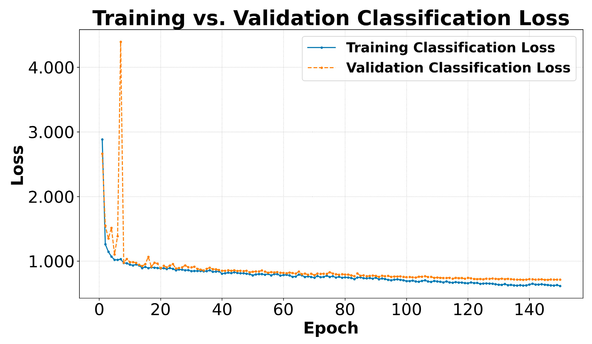
Figure 7 illustrates the Classification Loss. This loss quantifies the model's error in assigning the correct class to the detected objects. Both the Training and the Validation Box Loss consistently decrease. The validation curve closely follows the training curve, also stabilizing and suggesting good generalization capability for the classification task. YOLOv8 employs a loss function such as binary cross-entropy for this task, Eq. 4, [36]:
where the summation is performed on the classes used: attenuation_value, negative_value, pd_level_value, positive_pulse and voltage_value, and where:
- : Classification Loss value.
- : Ground truth label for class i. =1 if the object belongs to class i , =0 if it does not.
- : Probability predicted by the model that the object belongs to class i. It is the result of a sigmoid function with value in [0,1].
- : Natural logarithm.
Figure 7.
Comparison between Training Classification Loss and Validation Classification Loss.
3.1.4.3. Distribution Focal Loss
The DFL [37], shown in Figure 8, is a component that helps refine the prediction of bounding box coordinates by modeling the location of the box edges as a probability distribution. The training and validation DFL curves also show a decreasing trend and good correlation, indicating that the model is effectively learning this more detailed representation of the location.
The DFL is expressed in Eq. 5:
where:
- : DFL value.
- : Continue Ground truth coordinate of a box edge.
- : Label of the discrete container immediately to the left of y.
- : Label of the discrete container immediately to the right of y.
- : Probability predicted by the model for container
- : Probability predicted by the model for container .
- The terms and act as weights.
3.1.5. Performance Metrics
The model's performance was then evaluated using standard object detection metrics [38]. Specifically, the Precision, Recall, and Mean Average Precision metrics (mAP) were used. In all three cases, the growth was constant, and the stabilization of the metrics at high values indicates good detection and classification performance.
Precision and Recall in Training
Figure 9 and Figure 10 show the evolution of Precision, Eq. 6, and Recall, Eq. 7, respectively, othe training set. Both metrics tend to increase as training progresses, stabilizing at high values of 0.91 and 0.92 for Precision and Recall, respectively, indicating that the model learns to correctly identify relevant objects while minimizing false positives and false negatives in the analyzed data.
where TP are true positives, FP are false positives and FN are false negatives.
3.1.5.2. mAP in the Validation
The mAP is a key metric for evaluating the overall performance of object detectors. Figure 11 shows the mAP at an Intersection over Union (IoU) threshold of 0.5 (mAP@0.5), while Figure 12 presents the mAP averaged over multiple IoU thresholds from 0.5 to 0.95 in steps of 0.05 (mAP@0.5:0.95). Both mAP curves on the validation set show a steady increase, reaching values of 0.94 and 0.62 for (mAP@0.5) and (mAP@0.5:0.95), respectively. The more strict mAP@0.5:0.95 provides a more robust assessment of the model's localization performance. The steady growth and stabilization at high values indicate good detection and classification performance with validation data not seen in the training set.
The Average Precision (AP) for a class, Eq. 8, is calculated as the area under the Precision-Recall curve. One way to calculate it is:
where:
- : AP for a specific class.
- : Index of predictions ordered by confidence (from highest to lowest).
- : Total number of thresholds or data points considered.
- : Accuracy calculated at the kth Recall point or by considering the k highest confidence detections.
- : Change in Recall from point (k-1) to point k (i.e., .
3.2. Confusion Matrix
This section presents a detailed overview of the successes and errors of the classes that were considered through the study of the Confusion Matrix in the validation and in the test set.
3.2.1. Confusion Matrix on the Validation Set
The Confusion matrix [39], presented in Figure 13, provides a detailed view of the model’s classification successes for each of the five classes in the validation set. Values on the main diagonal represent correct classifications. A high number of correct predictions is observed for most classes: negative_pulse (650), positive_pulse (615), attenuation_value (145), pd_level_value (145), and voltage_value (144).
The attenuation_value, pd_level_value and voltage_value classes show very little confusion, indicating good distinction by the model. However, some confusions are identified in the background class, which is incorrectly classified as negative_pulse in 197 instances and as positive_pulse in 231 instances. Furthermore, instances of negative_pulse (98) and positive_pulse (87) are wrongly identified as background. These confusions could be due to the visual similarity of these signals with background noise or to the inherent variability of background signals, which can resemble weak pulses.
3.2.2. Confusion Matrix on the Test Set
After training the YOLOv8 model for 150 epochs, its detection and classification performance was evaluated on the test set, which consisted of 100 images not used during the training and validation phases. This set contains a total of 1,025 labeled object instances belonging to the five defined classes. The evaluated model, with 92 fused layers, 25,842,655 parameters, and a complexity of 78.7 GFLOPs, was subjected to inference on this dataset.
The model's processing speed on the test set was remarkable, with an average time of 1.7 ms for preprocessing, 11.3 ms for inference itself, and 5.3 ms for postprocessing per image. This results in an efficient overall inference time, which is crucial for applications requiring real-time responses or the processing of large volumes of data.
The overall evaluation results on the test set show robust model performance. An average Precision of 0.93 and an average Recall of 0.93 were obtained. Regarding the mAP, a value of 0.95 was achieved with an IoU threshold of 0.5 (mAP@0.5). When considering a stricter range of IoU thresholds, from 0.5 to 0.95 in steps of 0.05 (mAP@0.5:0.95), the model achieved a value of 0.62. These values suggest a good ability of the model to correctly locate and classify events in the signals, with mAP@0.5:0.95 being a stricter indicator of accuracy in locating bounding boxes.
Analyzing the performance broken down by class using the mAP@0.5:0.95 metric reveals the following values: attenuation_value 0.67, negative_pulse 0.45, pd_level_value 0.77, positive_pulse 0.48, and voltage_value 0.71.
Excellent performance is observed for the pd_level_value and voltage_value classes, followed by attenuation_value. The negative_pulse and positive_pulse classes exhibit lower mAP@0.5:0.95, indicating greater difficulty for the model in accurately localizing bounding boxes for these pulse types under strict IoU criteria, although its performance at mAP@0.5 remains high.
Figure 14 shows the confusion matrix obtained from the model's predictions on the test set. The following correct predictions are observed on the main diagonal: attenuation_value 99, negative_pulse 327, pd_level_value 99, positive_pulse 316, and voltage_value 99.
The attenuation_value, pd_level_value, and voltage_value classes show very little or no confusion with other classes or the background, indicating excellent distinction by the model for these specific events.
The model demonstrates a high ability to correctly classify most instances. However, some significant confusions are identified, primarily related to the background class. Specifically, the true background class is incorrectly classified as negative_pulse 76 times and as positive_pulse 86 times.
On the other hand, true instances of negative_pulse 47 and positive_pulse 37 are incorrectly classified as background. That is, in these cases, the model either fails to detect them or mistakes them for the background. There is also much less confusion between negative_pulse and positive_pulse, with just one instance of negative_pulse predicted as positive_pulse. Background confusion for positive and negative pulses could be attributed to the visual similarity of low amplitude pulses to background noise or to inherent variability in the signal that makes distinction difficult.
3.3. Inference in Operational Scenarios
This section analyzes the inference of images from the DDX electrical detector videos using the trained CNN. This automatically produces the five classes as the final result, and for three of them the numerical value is obtained.
3.3.1. Inference Flowchart
Figure 15 shows the flowchart that explains how inference is performed from video sequences from the DDX electrical detector for object detection and quantitative data extraction. The program was made in Python, and its architecture designed to be efficient and clear. It is divided into three phases: setup and initialization, frame-by-frame processing, and finalization.
Phase 1: Set up and initialization.
This is a preliminary phase that prepares all the components necessary for the analysis. It performs three tasks sequentially:
- Startup and configuration: the process begins by loading user-defined configurations, such as the input video and YOLOv8 model paths, confidence thresholds, and a list of interest classes that will trigger optical character recognition (OCR).
- Engine loading: the two main inference engines, the YOLOv8 object detection model and the Python EasyOCR OCR engine, are initialized and loaded into memory. This loading is performed only once at startup to optimize system performance. The number of GPUs to be used is also determined.
- Opening files: the input video stream is opened and the output files are created, including the new video with the visual annotations and the text file that will record its detailed data.
Phase 2: Frame by frame processing, main loop:
This is the operating core of the system, where each frame of the video is analyzed sequentially.
- YOLOv8 inference: the current frame is fed into the YOLOv8 model, which identifies and locates all classes of interest that exceed the confidence threshold, returning their bounding boxes, class labels, and confidence scores.
- Detection loop: the system iterates through each of the detections found in the frame.
- OCR class certification: for each detection, a decision is made based on its class label. If the class is predefined as an OCR target —pd_level_value, voltage_value, and attenuation_value— the system proceeds with OCR inference.
-
OCR inference: this critical step extracts the quantitative data:
- a.
- ROI cropping: the exact portion of the image contained within the detection bounding box is extracted from the frame.
- b.
- OCR application: the OCR engine analyzes this small ROI to recognize the textual information present.
- c.
- Value interpretation: the extracted text is processed to convert it into a numerical value.
- Output log: all detection data is logged. Bounding boxes and corresponding labels —confidence and OCR value, if applicable— are drawn on the output video frame. Detailed information about each detection, including the numerical value analyzed by the OCR, is added as a new line to the text file.
Phase 3: End
Once all frames have been processed, the system performs an orderly shutdown, leaving the output files ready for further analysis.
3.3.2. Results and Discussion
To test the performance and generalization capabilities of the YOLOv8 model trained and verified in the previous sections, an inference evaluation was performed on completely new data. To do this, three videos of 10 s were used, captured at voltage levels of 10 kV, 13 kV, and 16 kV, respectively. Each video, corresponding to approximately 300 images, was processed by the trained model to evaluate its effectiveness in detecting and classifying events under operating conditions not seen during training.
Figure 16 (a), (b), and (c) present representative frames of the inference for each voltage level. It is observed that the model not only successfully identifies the discharge pulses —negative_pulse and positive_pulse—, but also correctly reads and classifies the instrument numerical values —pd_level_value, voltage_value— and the attenuation value —attenuation_value. The high confidence scores, generally >0.70, for all classes demonstrate the robustness of the model in a complex task combining signal pattern detection with implicit optical character recognition.
For a deeper analysis of the relationship between PD activity and electrical magnitudes, cumulative detection images were generated for each 10 s video, as illustrated in Figure 17a, b and c. These images overlay all the bounding boxes of the detected pulses over the first frame of the video, providing a comprehensive view of the PD activity signature.
Analysis of these visualizations reveals a direct and physically consistent correlation between the applied voltage, the measured discharge level, and the activity detected by the model.
- At 10 kV, the model detects moderate discharge activity, with well-defined but relatively compact green clusters of negative and magenta positive pulses. This corresponds to an instrumental reading of PD Level 0.426 nC and Voltage 10.1 kV in Figure 17a.
- At 13 kV, with increasing voltage, a significant increase in the density and spatial extent of detections is observed. Both the negative and positive cumulative pulses are visibly larger and denser. This increased visual activity directly correlates with the increased discharge level measured by the instrument, which now shows PD Level 0.701 nC and Voltage 13.1 kV in Figure 17b.
- At 16 kV, the phenomenon intensifies dramatically. The cumulative image shows a much larger and more saturated area of activity, indicating a very severe PD regime. This exponential increase in visual activity is consistent with the instrumental reading, which reaches a PD Level of 3.88 nC and a Voltage of 16.6 kV, as shown in Figure 17c.
Table 1 presents a summary of the relationships between the main attributes obtained from the inference of the trained CNN for accumulated experiments at 10 kV, 13 kV and 16 kV. It presents the most significant Pearson correlation coefficients (r) [40], with a focus on the main electrical variables, ocr_voltage and ocr_pd_level, and their relationships with other geometric characteristics such as the pulse area, pulse coordinates CenterX and CenterY, as well as the number of positive and negative pulses detected. It shows a correlation of 0.90 between the magnitudes obtained in the ocr_voltage and ocr_pd_level classes, which confirms that these variables measure strongly related aspects of the same physical phenomenon.
We also observe a strong positive relationship of 0.77 between the increase in the magnitude of ocr_voltage and the number of pulse_negatives detected, suggesting that higher voltages generate more negative discharges. On the other hand, an inverse relationship is observed between voltage and the geometric ratio. The most notable negative correlation 0.41 is between ocr_voltage and Width. This indicates that pulses tend to become narrower as voltage increases. This is a non-obvious but highly informative pattern that the machine learning model is using for classification.
In conclusion, this experimental validation on data not used in the training set demonstrates the effectiveness of the trained model. Not only is it capable of generalizing and operating as a robust monitoring system, but its visual detections act as a qualitative and quantitative analogue of electrical measurements. The density, area, and frequency of bounding boxes detected by the model provide a direct visual measure of the severity of the phenomenon, validating this approach as a powerful and reliable tool for the automated diagnosis and quantification of PDs.
4. CNN Training and Inference from HQ Images
This section presents the CNN training and inference analysis in operational scenarios using images obtained using the HQ camera. The training environment in this section is the same as that used in Section 3. However, in this section a semi-automatic generation of the dataset is realized, which greatly facilitates the labeling of the training, validation, and test sets.
4.1. CNN Training
The purpose of this section is to train a CNN based on YOLOv8 architecture. The section is divided into two subsections: semi-automatic dataset generation and training results.
4.1.1. Semi-Automatic Generation of the Dataset
To train the CNN based on the YOLOv8 architecture for PD detection in videos obtained with the HQC, a Python script was developed for video processing to obtain the training, validation, and test images. This process automates the identification of candidate events, filters out known false positives, and generates a structured and labeled dataset in the format required by YOLOv8. The methodology is based on background subtraction, contour analysis, and a novel manual spatial exclusion filter that significantly improves the quality of the final dataset by reducing noise and the need for subsequent manual cleaning.
The structure of this section is as follows: first, the semi-automatic data acquisition model is configured and initialized. Next, a Python program is created for PD detection and extraction. Data filtering, validation, and collection are then performed. Finally, the dataset is generated in YOLOv8 format for CNN training. To facilitate understanding of this process, a flowchart summarizing the overall method described is included.
Configuration and Initialization
The process begins with a configuration phase where key parameters are defined. The I/O paths are defined first, and then the input video and output file paths are specified. These include debugging videos —difference, threshold and detected events— and a .dat data file with the characteristics of each PD.
Manual exclusion zones are then established. This is a crucial component of the system as it allows the user to define a priori spatial regions in the image where recurring false positives —reflections, sensor noise, etc.— are known to occur. Each zone is defined by a centroid, an exclusion radius on the x and y axes, and, optionally, an expected area with its tolerance. Any detected event whose centroid falls within one of these zones is automatically discarded.
The parameters of YOLOv8 dataset are defined below. The dataset's root directory, the class to be detected (PD), and the ratios for dividing the data into training sets, 66.7%, validation sets, 22.0%, and test sets, 11.3%, are named.
PD Detection and Extraction
The core of the Python script processes the video frame by frame to identify events of interest. This process is broken down into four steps:
- Background establishment: the first frame of the video is assumed to represent the static background of the scene. This frame is converted to grayscale and stored for reference.
- Background subtraction: for each subsequent frame, the absolute difference with the background frame is calculated. The result is an image that highlights only the regions where changes have occurred (i.e., new PD).
- Thresholding and morphological cleaning: the resulting image is binarized using a fixed threshold to convert subtle changes into well-defined, white-on-black regions. A morphological operation is then applied to remove noise.
- Contour detection: on this last image, the OpenCV Python library algorithm [19] is applied to determine the contours of all the change regions. Each contour represents a candidate PD.
Filtering, Validation and Data Collection
This process is carried out in the following steps:
- Minimum area filter: contours with an area smaller than a predefined threshold of 5 pixels are discarded to remove residual noise.
- Manual exclusion filter: the contour centroid is calculated. If this centroid falls within any of the manual exclusion zones defined in the configuration, the contour is classified as a false positive and discarded.
- Data collection: if a contour passes both of the above filters, it is considered a valid PD.
- For each valid PD, the following is extracted and stored:
- The bounding box.
- The centroid coordinates, area and average RGB color intensity in a .dat text file for further analysis.
- A copy of the original, unprocessed frame and the list of bounding boxes for all valid events found are saved. This pair (image, labels) is the input data in YOLOv8 format.
Generating the Dataset in YOLOv8 Format
- Once the entire video has been processed, the script uses the collection of frames with valid PDs to build the final dataset and the following steps are performed:
- Directory structuring: a folder structure compatible with YOLOv8 framework is created with the subdirectories train, valid, and test, each containing folders for images and labels.
- Data splitting: the data collection —images and their labels— is randomly shuffled and split into training, validation, and test sets according to the ratios defined above.
- File generation for each image: the original image is saved as an image_name.jpg in the corresponding images folder.
- An image_label.txt file is created in the corresponding labels folder. Within this file, each line represents an event detected in that image, in the format: [class_index, x_center_norm, y_center_norm, width_norm, height_norm]. All bounding box coordinates are normalized by dividing them by the frame width and height dimensions, as required by YOLOv8.
- Configuration file (data.yaml): finally, a data.yaml file is generated at the root of the dataset. This file is essential for YOLOv8 to locate the datasets and identify the number of classes and their names.
The end result is a high-quality dataset, ready to be used directly in training a YOLOv8 object detection model, minimizing manual intervention and improving labeling consistency.
Summary Flowchart of the Process
To visualize the logical flow of the script used to generate the YOLOv8 compatible dataset, a flowchart was created as shown in Figure 18.
The three main phases of the flowchart are summarized below:
- Setup and loading: in this initial phase, all resources are prepared. The script reads the file paths, uploads the video, and manually defines exclusion zones, which are key to filtering out known false positives.
- Video processing loop: this is the core of the script. It operates frame by frame, performing two main tasks in sequence:
2a) PD detection and filtering: this block encapsulates all the computer vision logic, subtracts the background (see Figure 19a) to find the changes that occur, binarizes the image, finds the PD boundaries and applies filters, both the minimum area filter and the manual exclusion zones filter.
2b) Temporary storage: if a frame contains at least one PD that has passed all filters, the script saves the original image of that frame along with the coordinates of the bounding boxes (see Figure 19b and c of the valid PD).
- 3.
- YOLOv8 dataset generation: once the entire video has been analyzed, this final phase takes all the valid data collected and organizes it into the folder structure and file formats required by YOLOv8. This includes splitting the data into training/validation/test sets, normalizing the coordinates, and creating the .yaml configuration file.
4.1.2. Training Results
Three image series were used to train the CNN. The PD series occurring within the dielectric oil correspond to an average voltage of 10 kV, 13 kV, and 16 kV, respectively. The total dataset consists of 4,457 images, managed and labeled using the semi-automatic system explained in the flowchart represented in Figure 18. For the training and evaluation process, the dataset was divided into three subsets:
- Training set: 2,967 images.
- Validation set: 982 images.
- Test set: 508 images.
The training environment is the same as for the DDX image training seen in Section 3. The YOLOv8 model was trained in four iterations: the first and second with 100 epochs, the third with 200, and the fourth, to ensure convergence, with 523. Some images from this dataset with box labeling in YOLOv8 format can be seen in Figure 19b and c. The training speed is 18.9 s per epoch. This demonstrates a very fast experimentation cycle, allowing for efficient model iteration and tuning.
The implemented object detector is based on a deep CNN architecture optimized for inference. The model consists of 92 fused computational layers, a technique that improves speed by combining operations such as convolution and batch normalization. With a total of 25,840,339 parameters, the model has a high capacity to learn and represent the complex visual characteristics of the PD of interest. Its computational load is quantified at 78.7 GFLOPs, a key metric that indicates the required processing demand and positions the model as a robust solution, suitable for running on GPU-accelerated hardware.
The evolution of performance metrics during training provides crucial information about the model's learning process. Figure 20a and b depict the Training vs. Validation Box Loss and Classification Loss curves, respectively. Figure 21a and b illustrate the Training vs. Validation DFL Loss and Training Precision curves over 520 epochs, consisting of 982 images.
Consistent behavior is observed across the three loss graphs: Box Loss, Classification Loss, and DFL Loss. During the first 375 epochs, the model demonstrates an effective learning phase. The loss curves for both training (solid blue line) and validation (dashed orange line) slope downward simultaneously. This indicates that the model is generalizing correctly, improving its ability to locate Box Losses, correctly classify PD (Classification Loss), and refine the DFL Loss on unseen data.
However, starting at epoch 375, a clear inflection point becomes evident, signaling the onset of overfitting. While the training set loss continues its downward trend, the three validation set loss metrics reverse their trajectory and begin to increase steadily. This phenomenon is a classic indicator that the model has begun to memorize the specific characteristics and noise of the training set, losing its ability to generalize to new data. Therefore, the model with the best performance is not the one obtained at the end of training, but the one whose weights correspond to the minimum point of the validation loss, around epoch 375.
Regarding Precision, the graph in Figure 21b shows its evolution on the training set, where it stabilizes at an average value close to 0.77. This behavior suggests that, even on the training data, the model does not achieve perfect accuracy. This can be attributed to the nature of the dataset, which likely contains a subset of PDs that are intrinsically difficult to detect, such as very small-area or low-contrast PDs. The model assigns a lower confidence score to these complex detections which, when averaged over the entire set, results in an accuracy metric that does not reach higher values. The constant fluctuation in the accuracy curve reflects the model's continuous effort to adjust its predictions to this PD variability.
In conclusion, the analysis of the training curves confirms the attainment of a functional model, but also underscores the critical importance of employing an early stopping strategy or selecting the model based on the minimum validation loss to avoid deploying an overfitted and underperforming model in real-world applications.
4.2. Inference in Operational Scenarios
Once the CNN was trained, the model's performance was evaluated on the inference task using three independent test videos, corresponding to PDs generated under voltages of 10 kV, 13 kV, and 16 kV. The model's efficiency is remarkable, with an inference time of just 1.2 ms per frame. This translates into a theoretical processing capacity of approximately 833 FPS, confirming its suitability for real-time applications or for analyzing large volumes of video.
Figure 22 shows examples of inference on individual frames for each voltage level. The model is observed to correctly identify PDs under all conditions. The variability in the assigned confidence scores is notable. While events at 10 kV and 13 kV are detected with high confidence (0.91), 16 kV receives a more dispersed range of scores (0.92, 0.84, and even 0.39 for a weaker PD). This behavior is consistent with the analysis of the training accuracy curve and demonstrates the model's ability to quantify the certainty of its own detections.
A more in-depth analysis is obtained by accumulating all detections over each video, lasting 45 s in this case. Figure 23 provides a visualization of the accumulated PD density over the image. In addition, Figure 24, Figure 25 and Figure 26 provide a detailed analysis of their spatial distribution, area and detection confidence.
The following conclusions can be drawn:
- a)
- Correlation between voltage and discharge activity: there is a clear relationship between the voltage applied to the electrodes and the number of detected PDs. At 10 kV, 1,582 PDs were accumulated (Figure 23a). As the voltage is increased to 13 kV, the activity increases significantly, recording 2,050 PDs (Figure 23b). However, at 16 kV, the total number of detected PD drops slightly to 1,981 (Figure 23c). A reasonable hypothesis for this small decrease is that at higher energies the PDs are larger and may merge, being detected by the model as a single PD with a larger area instead of multiple smaller PDs.
- b)
- Spatial expansion of activity: the scatter plots shown in Figure 24, Figure 25 and Figure 26 visually confirm that the area of discharge activity expands with increasing voltage. The cluster of points, initially highly concentrated in the dielectric space at 10 kV, expands both vertically and horizontally at 13 kV and, more pronouncedly, at 16 kV. This suggests that at higher voltage levels in the dielectric, PDs are not only more frequent but also occupy a larger volume.
- c)
-
Increasing the detection area and correlation with PD confidence: the most revealing analysis comes from the direct comparison between the area and confidence of the PD in Figure 24, Figure 25 and Figure 26:
- Area distribution (Figure 24a, Figure 25a and Figure 26a): at 10 kV, the vast majority of PDs are small in area (blue and green dots). At 13 kV, a slight increase in the average area is observed. The change is important at 16 kV, where a significant presence of large-area PDs appears, represented by yellow and orange colors.
- Confidence distribution (Figure 24b, Figure 25b and Figure 26b): complementarily, the analysis of detection confidence provides a new layer of information. A strong positive correlation is observed between the area of a PD and the confidence with which it is detected. Larger PDs with warm colors in Figure 24a, Figure 25a and Figure 26a consistently correspond to high-confidence detections, with warm colors close to 1.0 in Figure 24b, Figure 25b and Figure 26b. This is physically consistent. Larger and more energetic PDs are visually clearer and therefore more confidently identified by the model. Conversely, low-confidence points –cool colors in Figure 24b, Figure 25b and Figure 26b– tend to correspond to smaller PDs, which are harder to distinguish from background noise.
5. Conclusions
This work presents an innovative bimodal approach for laboratory PD analysis through training of a CNN based on YOLOv8.
Firstly, a conventional DDX-type PD electrical detector is enhanced by endowing it with smart capabilities. A system is developed capable of automatically reading and interpreting data displayed on the electrical detector screen, such as discharge magnitude, pulse count, and applied voltage. In this way we transform a passive conventional instrument into a smart and autonomous source of digitized and structured data. The mean precision in the training was 0.91
Concurrently, an optical visualization system using a high quality camera is employed to capture direct images of PDs occurring in the dielectric oil. In addition, the training dataset for the camera is generated semi-automatically using a Python program. These images provide complementary qualitative and quantitative information, enabling the classification of discharge types based on their visual characteristics. This offers a new and complementary dimension providing the spatial location and morphology of PDs. Image analysis makes it possible to identify exactly where the PDs originate and how they propagate between the electrodes, vital information for diagnosing the exact point of failure or insulation degradation. For electrical voltages of 10 kV, 13 kV and 16 kV, PDs were detected with confidence scores of up to 0.92.
This synergy offers a more complete, accurate, and automated diagnosis of PD behavior in dielectric oils, improving the understanding of degradation mechanisms and the operational reliability of electrical assets. In this way, both systems, operating in parallel, enhance each other. The DDX electrical detector quantifies the charge, providing a measure of the magnitude of the problem, while the optical detector finds the location of the source of the problem. The fusion of this bimodal information, the electrical magnitude and the spatiotemporal distribution, allows for a much more complete and robust diagnosis of the dielectric insulation oil condition than could be achieved with either system alone. This approach represents a significant advance toward smarter and more accurate monitoring systems, capable of not only detecting the presence of PDs but also identifying their root cause and predicting failures more effectively.
Supplementary Materials
The following supporting information can be downloaded at: the provisionally link: https://zenodo.org/records/16890497?preview=1&token=eyJhbGciOiJIUzUxMiJ9.eyJpZCI6ImJiMzM3ZjI2LWY3YzctNDhlMy05ZDQxLWE3NGYwZGVhOTNjNCIsImRhdGEiOnt9LCJyYW5kb20iOiIyZjA0MDQzOTllNzg4NTM3YTZhOTk5MzRhMjJjNmU2MiJ9.ry2VGmh_5MbpiBbnrfb64Z6C7yhWo094jDA1xgPNWOEFyF6KZIggFhUXFNKEyTGcqtyipnZ88y6FI2ugCim35Q, Software and dataset of Fusion of electrical and optical methods in the detection of partial discharges in dielectric oils using YOLOv8.
Author Contributions
J.M.M.-V. supported the theory background, collected and processed the images, developed the experiments, analyzed the data, and wrote the paper. S.G.-A. and F.J.S.-M. supported the theory background, analyzed the data, and wrote the paper. All authors have read and agreed to the published version of the manuscript.
Funding
This research received no external funding.
Data Availability Statement
Data are contained within the article.
Acknowledgments
We wish to acknowledge the Institute for Applied Microelectronics, the Electrical Engineering Department, and the Department of Electronic Engineering and Automatics at the University of Las Palmas de Gran Canaria.
Conflicts of Interest
The authors declare no conflicts of interest.
References
- Saravanan, B.; D, P. K. M.; Vengateson, A. Benchmarking Traditional Machine Learning and Deep Learning Models for Fault Detection in Power Transformers, 2025. https://arxiv.org/abs/2505.06295.
- Zhang, R.; Zhang, Q.; Zhou, J.; Wang, S.; Sun, Y.; Wen, T. Partial Discharge Characteristics and Deterioration Mechanisms of Bubble-Containing Oil-Impregnated Paper. IEEE Trans. Dielectr. Electr. Insul. 2022, 29, 1282–1289. [Google Scholar] [CrossRef]
- IS IEC 60270:2000AMD1:2015 CSV; High-Voltage Test Techniques—Partial Discharge Measurements. Edition 3.1, 2015–11. Consolidated Version. International Electrotechnical Commission: Geneva, Switzerland, 2015.
- Thobejane, L. T.; Thango, B. A. Partial Discharge Source Classification in Power Transformers: A Systematic Literature Review. Appl. Sci. 2024, 14. [Google Scholar] [CrossRef]
- Madhar, S. A.; Mor, A. R.; Mraz, P.; Ross, R. Study of DC Partial Discharge on Dielectric Surfaces: Mechanism, Patterns and Similarities to AC. Int. J. Electr. Power Energy Syst. 2021, 126, 106600. [Google Scholar] [CrossRef]
- Wotzka, D.; Sikorski, W.; Szymczak, C. Investigating the Capability of PD-Type Recognition Based on UHF Signals Recorded with Different Antennas Using Supervised Machine Learning. Energies 2022, 15. [Google Scholar] [CrossRef]
- Sikorski, W. Development of Acoustic Emission Sensor Optimized for Partial Discharge Monitoring in Power Transformers. Sensors 2019, 19. [Google Scholar] [CrossRef] [PubMed]
- Shahsavarian, T.; Pan, Y.; Zhang, Z.; Pan, C.; Naderiallaf, H.; Guo, J.; Li, C.; Cao, Y. A Review of Knowledge-Based Defect Identification via PRPD Patterns in High Voltage Apparatus. IEEE Access 2021, 9, 77705–77728. [Google Scholar] [CrossRef]
- Khan, M. A. M. AI AND MACHINE LEARNING IN TRANSFORMER FAULT DIAGNOSIS: A SYSTEMATIC REVIEW. Am. J. Adv. Technol. Eng. Solut. 2025, 1, 290–318. [Google Scholar] [CrossRef]
- Khaleghi, B.; Khamis, A.; Karray, F. O.; Razavi, S. N. Multisensor Data Fusion: A Review of the State-of-the-Art. Inf. Fusion 2013, 14, 28–44. [Google Scholar] [CrossRef]
- Deng, X.; Jiang, Y.; Yang, L. T.; Lin, M.; Yi, L.; Wang, M. Data Fusion Based Coverage Optimization in Heterogeneous Sensor Networks: A Survey. Inf. Fusion 2019, 52, 90–105. [Google Scholar] [CrossRef]
- Xing, Z.; He, Y. Multi-Modal Information Analysis for Fault Diagnosis with Time-Series Data from Power Transformer. Int. J. Electr. Power Energy Syst. 2023, 144, 108567. [Google Scholar] [CrossRef]
- Guo, J.; Zhao, S.; Huang, B.; Wang, H.; He, Y.; Zhang, C.; Zhang, C.; Shao, T. Identification of Partial Discharge Based on Composite Optical Detection and Transformer-Based Deep Learning Model. IEEE Trans. Plasma Sci. 2024, 52, 4935–4942. [Google Scholar] [CrossRef]
- Yin, K.; Wang, Y.; Liu, S.; Li, P.; Xue, Y.; Li, B.; Dai, K. GIS Partial Discharge Pattern Recognition Based on Multi-Feature Information Fusion of PRPD Image. Symmetry 2022, 14. [Google Scholar] [CrossRef]
- Abubakar, A.; Zachariades, C. Phase-Resolved Partial Discharge (PRPD) Pattern Recognition Using Image Processing Template Matching. Sensors 2024, 24. [Google Scholar] [CrossRef] [PubMed]
- Dempster, A. P. Upper and Lower Probabilities Induced by a Multivalued Mapping. In Classic Works of the Dempster-Shafer Theory of Belief Functions; Yager, R. R., Liu, L., Eds.; Springer Berlin Heidelberg: Berlin, Heidelberg, 2008. [Google Scholar] [CrossRef]
- Sentz, S., K. &. Ferson. Combination of Evidence in Dempster-Shafer Theory, 2002. https://www.stat.berkeley.edu/~aldous/Real_World/dempster_shafer.pdf. (accessed on 21 July 2025).
- Redmon, J.; Divvala, S.; Girshick, R.; Farhadi, A. You Only Look Once: Unified, Real-Time Object Detection, 2016. https://arxiv.org/abs/1506.02640.
- Opencv-Python 4.12.0.88. https://pypi.org/project/opencv-python/. (accessed on 21 July 2025).
- Redmon, J.; Farhadi, A. YOLO9000: Better, Faster, Stronger, 2016. https://arxiv.org/abs/1612.08242.
- Redmon, J.; Farhadi, A. YOLOv3: An Incremental Improvement, 2018. https://arxiv.org/abs/1804.02767.
- Bochkovskiy, A.; Wang, C.-Y.; Liao, H.-Y. M. YOLOv4: Optimal Speed and Accuracy of Object Detection, 2020. https://arxiv.org/abs/2004.10934.
- Ultralytics. Ultralytics/Yolov5: V7.0 - YOLOv5 SOTA Realtime Instance Segmentation, 2022. [CrossRef]
- Li, C.; Li, L.; Jiang, H.; Weng, K.; Geng, Y.; Li, L.; Ke, Z.; Li, Q.; Cheng, M.; Nie, W.; Li, Y.; Zhang, B.; Liang, Y.; Zhou, L.; Xu, X.; Chu, X.; Wei, X.; Wei, X. YOLOv6: A Single-Stage Object Detection Framework for Industrial Applications, 2022. https://arxiv.org/abs/2209.02976.
- Wang, C.-Y.; Bochkovskiy, A.; Liao, H.-Y. M. YOLOv7: Trainable Bag-of-Freebies Sets New State-of-the-Art for Real-Time Object Detectors, 2022. https://arxiv.org/abs/2207.02696.
- Jocher, G.; Qiu, J.; Chaurasia, A. Ultralytics YOLO, 2023. https://github.com/ultralytics/ultralytics.
- Terven, J.; Córdova-Esparza, D.-M.; Romero-González, J.-A. A Comprehensive Review of YOLO Architectures in Computer Vision: From YOLOv1 to YOLOv8 and YOLO-NAS. Mach. Learn. Knowl. Extr. 2023, 5, 1680–1716. [Google Scholar] [CrossRef]
- Alif, M. A. R.; Hussain, M. YOLOv1 to YOLOv10: A Comprehensive Review of YOLO Variants and Their Application in the Agricultural Domain, 2024. https://arxiv.org/abs/2406.10139.
- Kang, S.; Hu, Z.; Liu, L.; Zhang, K.; Cao, Z. Object Detection YOLO Algorithms and Their Industrial Applications: Overview and Comparative Analysis. Electronics 2025, 14, 1104. [Google Scholar] [CrossRef]
- Reis, D.; Kupec, J.; Hong, J.; Daoudi, A. Real-Time Flying Object Detection with YOLOv8, 2024. https://arxiv.org/abs/2305.09972.
- Monzón-Verona, J. M.; González-Domínguez, P.; García-Alonso, S. Characterization of Partial Discharges in Dielectric Oils Using High-Resolution CMOS Image Sensor and Convolutional Neural Networks. Sensors 2024, 24. [Google Scholar] [CrossRef] [PubMed]
- Raspberry Pi HQ Camera. Available online: https://www.raspberrypi.com/documentation/accessories/camera.html#hq-camera (accessed on 17 June 2025).
- Rasband, W. ImageJ, 1997. https://imagej.net/ij/. (accessed on 21 July 2025).
- Roboflow. Available online: https://www.roboflow.com (accessed on 21 July 2025).
- Zheng, Z.; Wang, P.; Liu, W.; Li, J.; Ye, R.; Ren, D. Distance-IoU Loss: Faster and Better Learning for Bounding Box Regression. Proc. AAAI Conf. Artif. Intell. 2020, 34, 12993–13000. [Google Scholar] [CrossRef]
- Janocha, K.; Czarnecki, W. M. On Loss Functions for Deep Neural Networks in Classification, 2017. https://arxiv.org/abs/1702.05659.
- Li, X.; Wang, W.; Wu, L.; Chen, S.; Hu, X.; Li, J.; Tang, J.; Yang, J. Generalized Focal Loss: Learning Qualified and Distributed Bounding Boxes for Dense Object Detection, 2020. https://arxiv.org/abs/2006.04388.
- Lin, T.-Y.; Maire, M.; Belongie, S.; Hays, J.; Perona, P.; Ramanan, D.; Dollár, P.; Zitnick, C. L. Microsoft COCO: Common Objects in Context. In Computer Vision – ECCV 2014; Fleet, D., Pajdla, T., Schiele, B., Tuytelaars, T., Eds.; Springer International Publishing: Cham, 2014; pp. 740–755. [Google Scholar]
- Che, Q.; Wen, H.; Li, X.; Peng, Z.; Chen, K. P. Partial Discharge Recognition Based on Optical Fiber Distributed Acoustic Sensing and a Convolutional Neural Network. IEEE Access 2019, 7, 101758–101764. [Google Scholar] [CrossRef]
- Rodgers, J. L.; Nicewander, W. A. Thirteen Ways to Look at the Correlation Coefficient. Am. Stat. 1988, 42, 59–66. [Google Scholar] [CrossRef]
Figure 1.
Transparent methacrylate cell with the two electrodes.
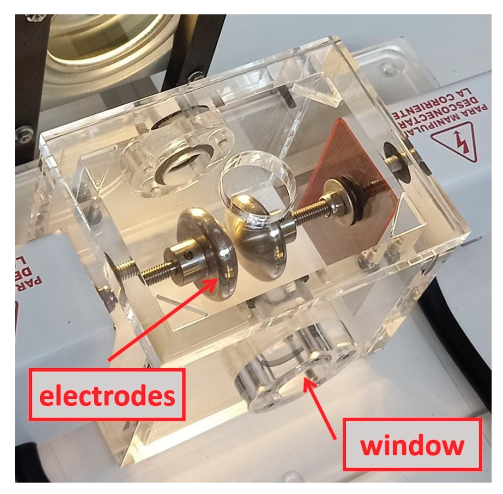
Figure 2.
(a) Operating terminal OT 248 system, Tettex-Haefely test AG. (b) PD detector DDX-9101, Tettex-Haefely test AG.
Figure 2.
(a) Operating terminal OT 248 system, Tettex-Haefely test AG. (b) PD detector DDX-9101, Tettex-Haefely test AG.
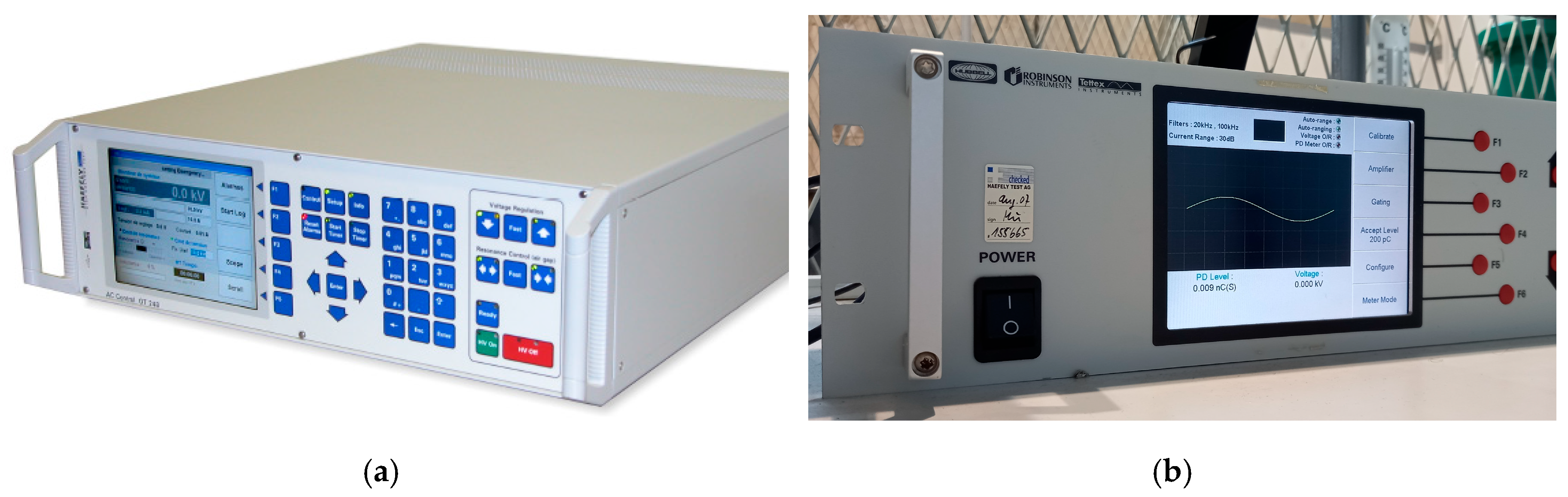
Figure 3.
Position of the HQC and schematic of the experimental setup.
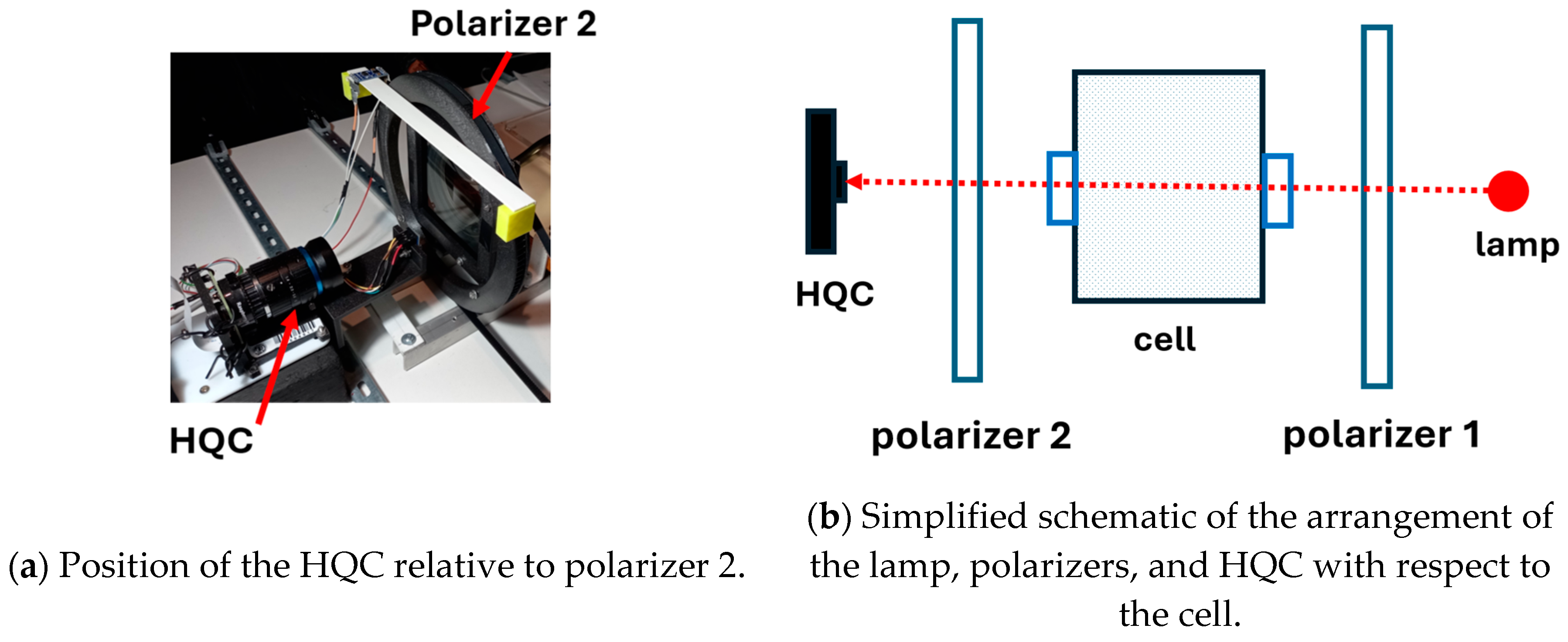
Figure 4.
Images collected by the DDX for voltages from 6 to 16 kV.
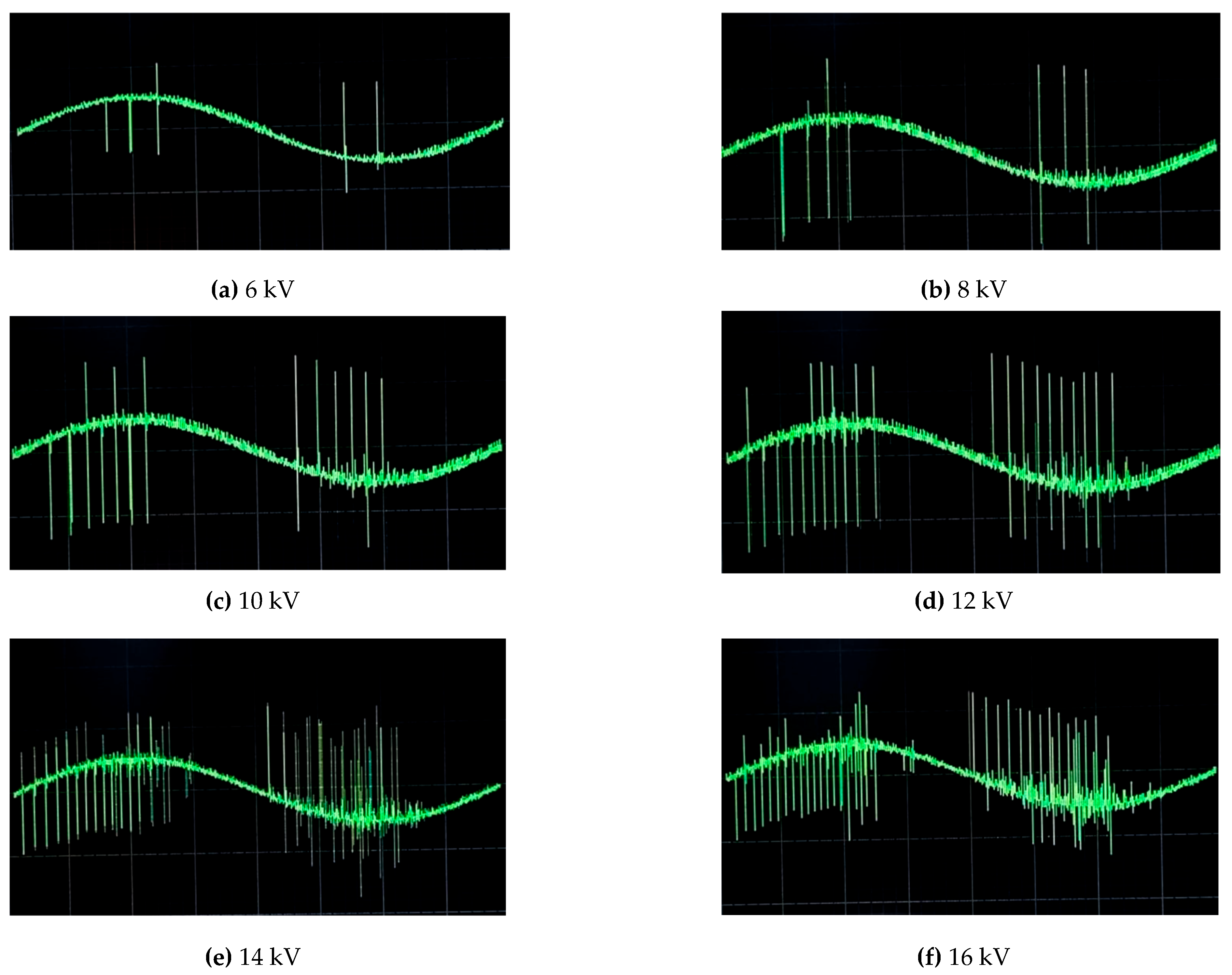
Figure 5.
ROI labeling with Roboflow showing the five classes used: attenuation_value, negative_value, pd_level_value, positive_pulse, and voltage_value.
Figure 5.
ROI labeling with Roboflow showing the five classes used: attenuation_value, negative_value, pd_level_value, positive_pulse, and voltage_value.
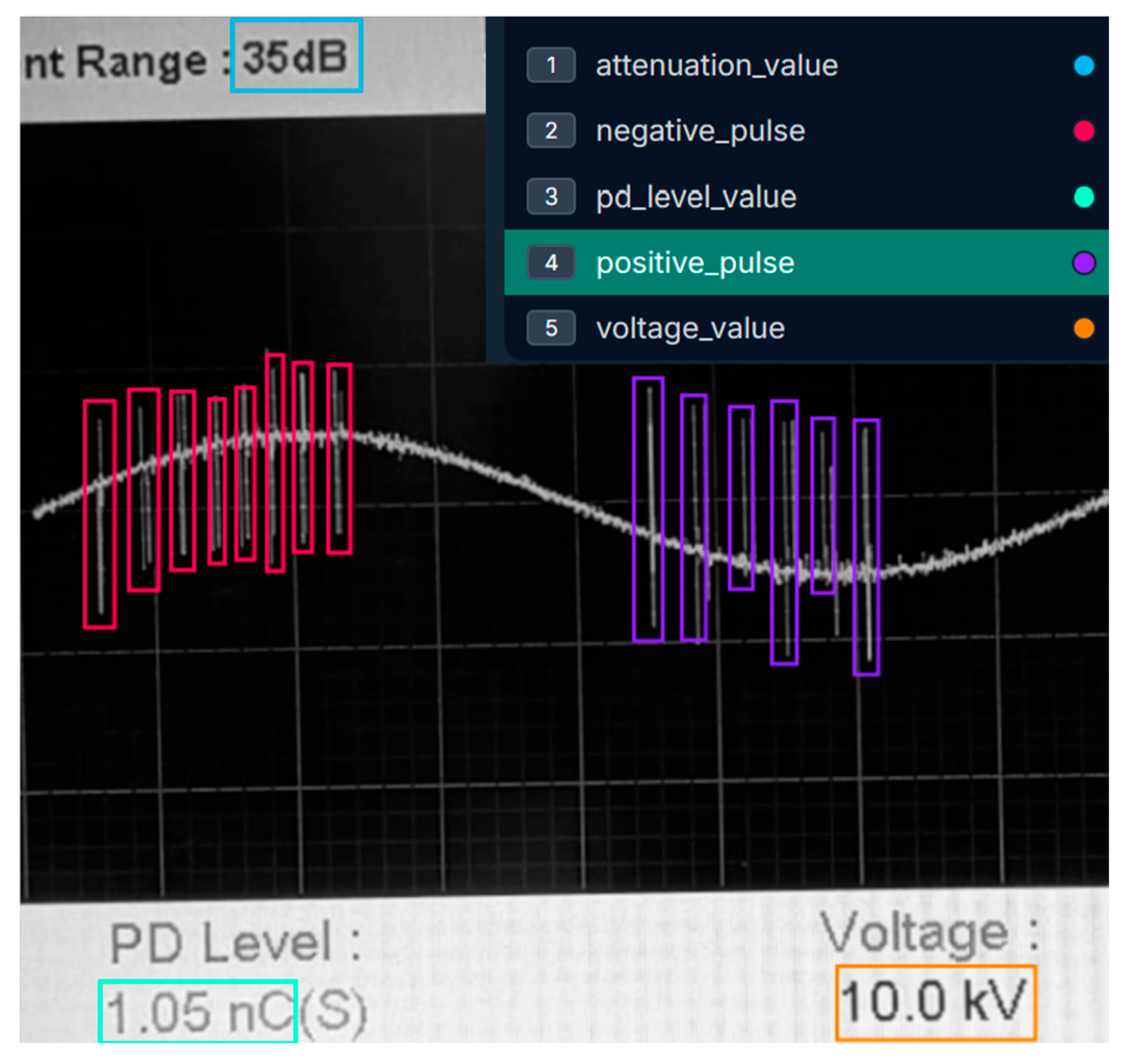
Figure 6.
Comparison between Training Box Loss and Validation Box Loss.
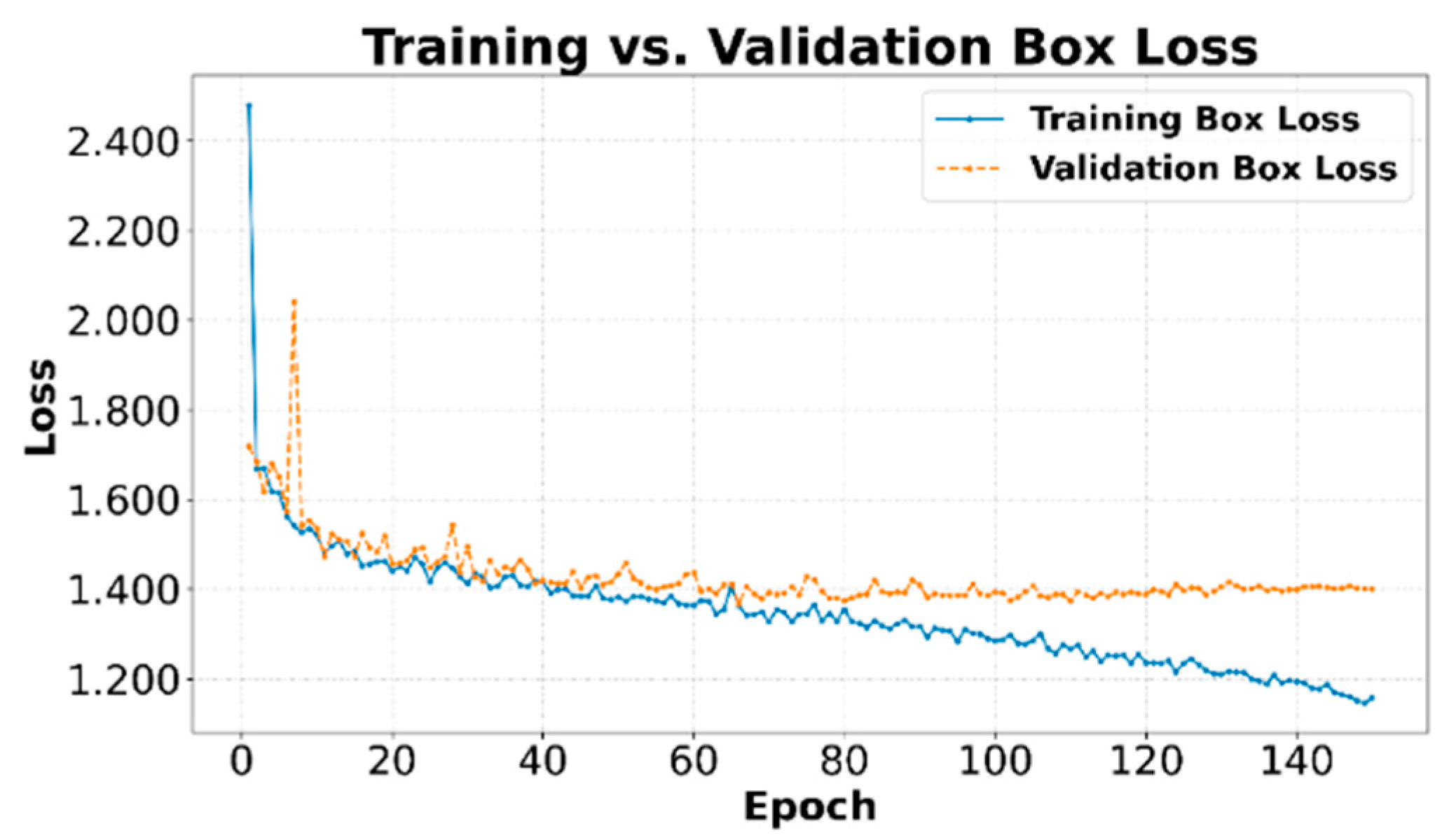
Figure 8.
Comparison between Training and Validation DFL Loss.
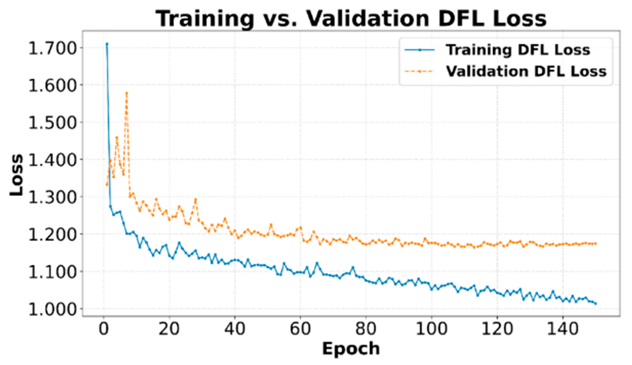
Figure 9.
Precision on the training set.
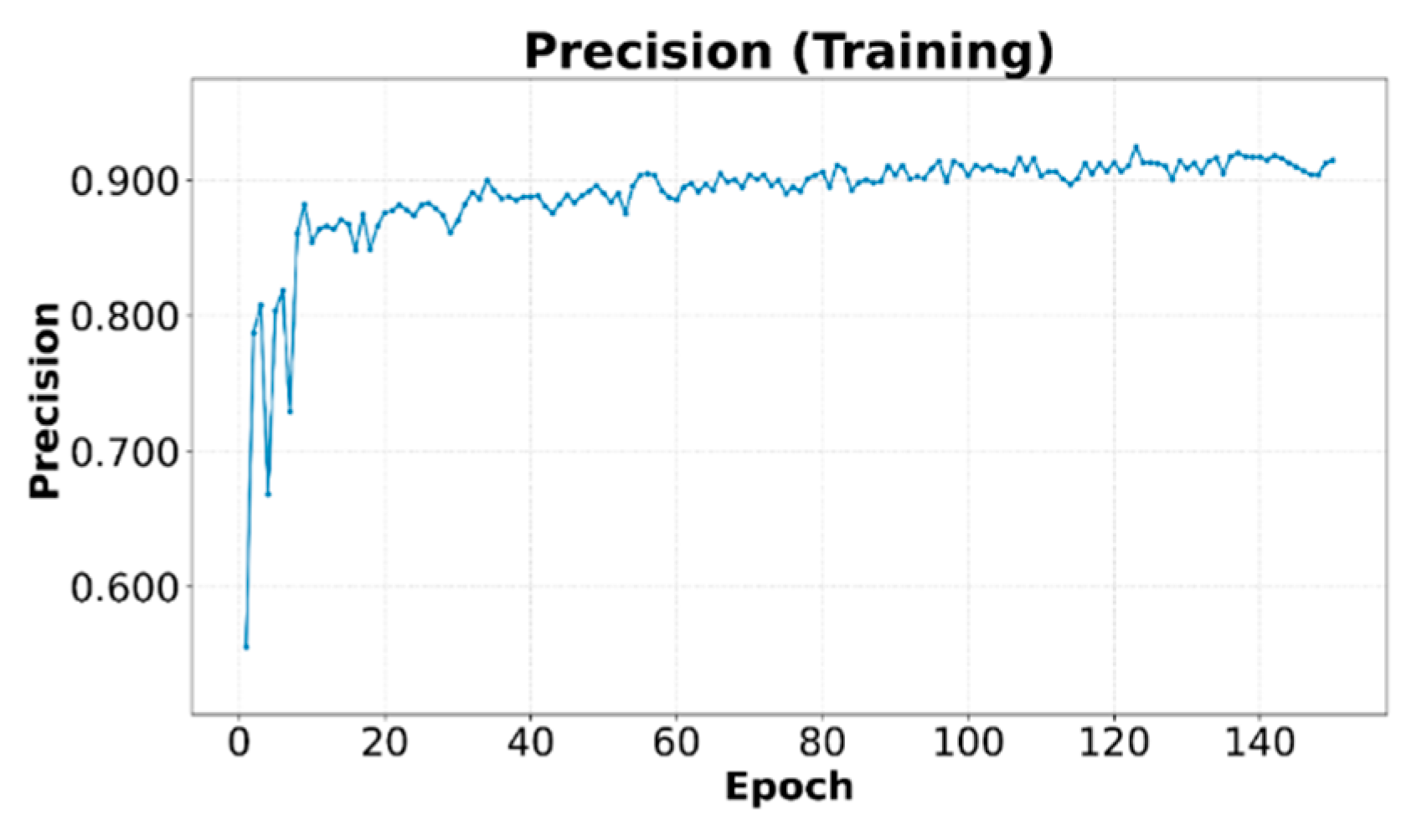
Figure 10.
Recall on the training set.
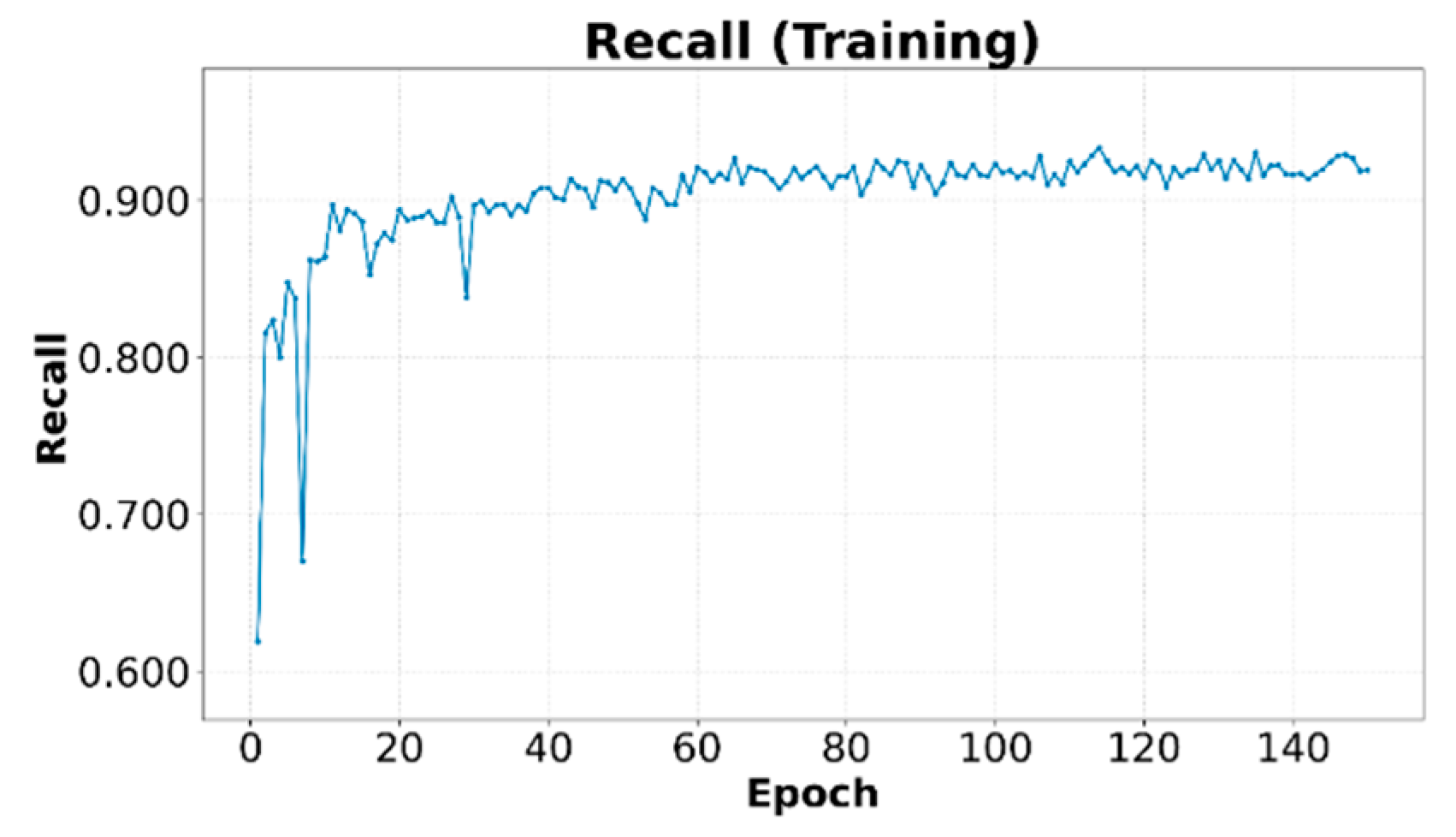
Figure 11.
mAP@0.5 on the validation set.
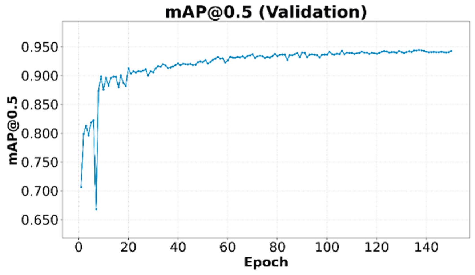
Figure 12.
mAP@0.5:0.95 on the validation set.
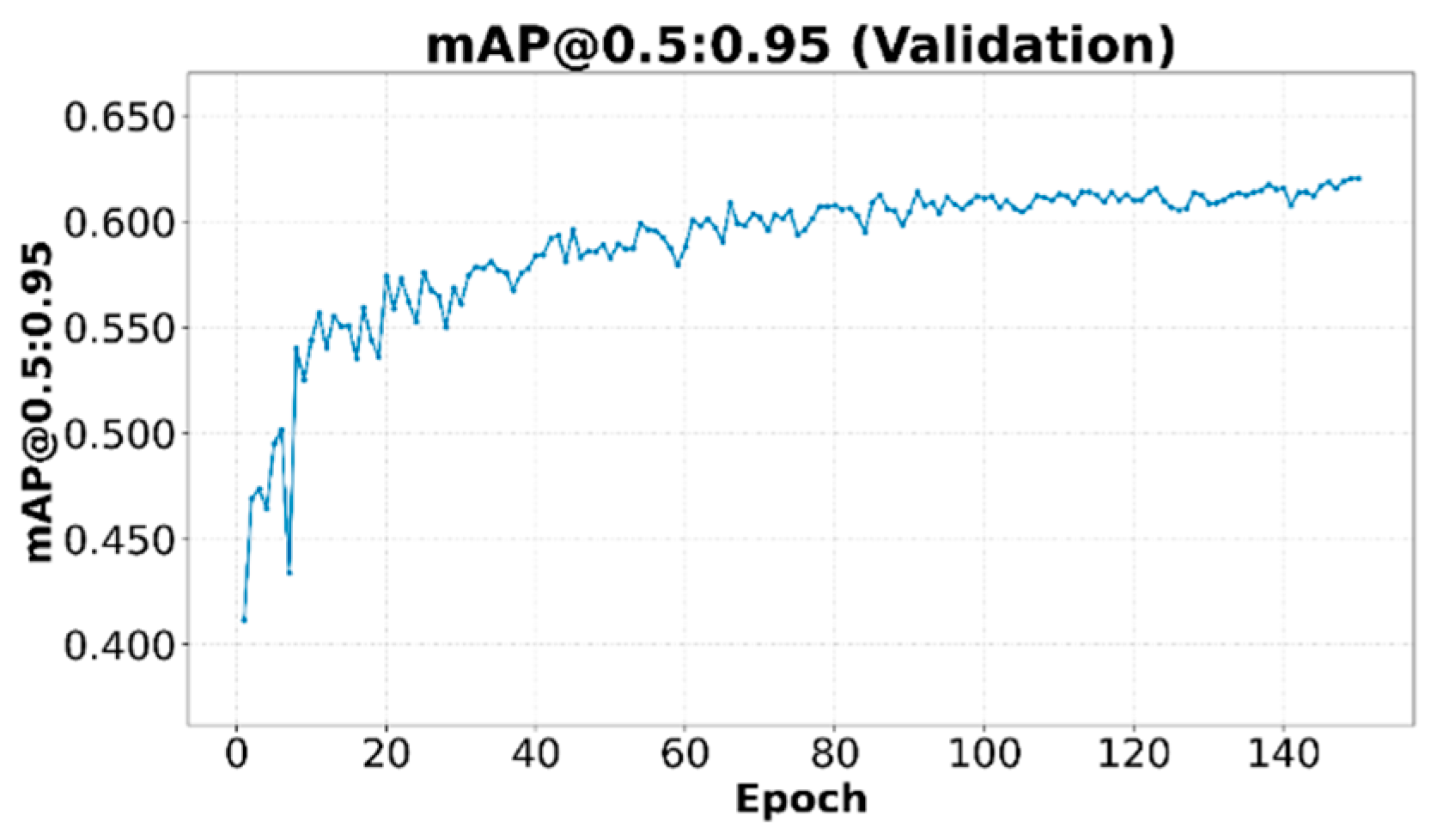
Figure 13.
Confusion matrix of the model on the validation set.
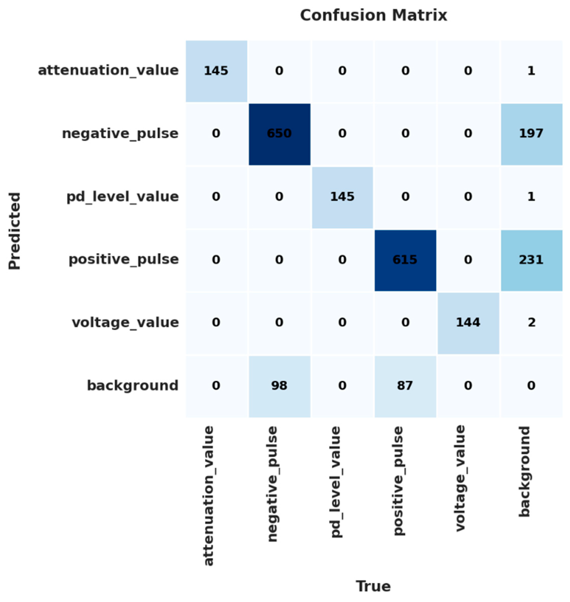
Figure 14.
Confusion matrix model predictions on the test set.
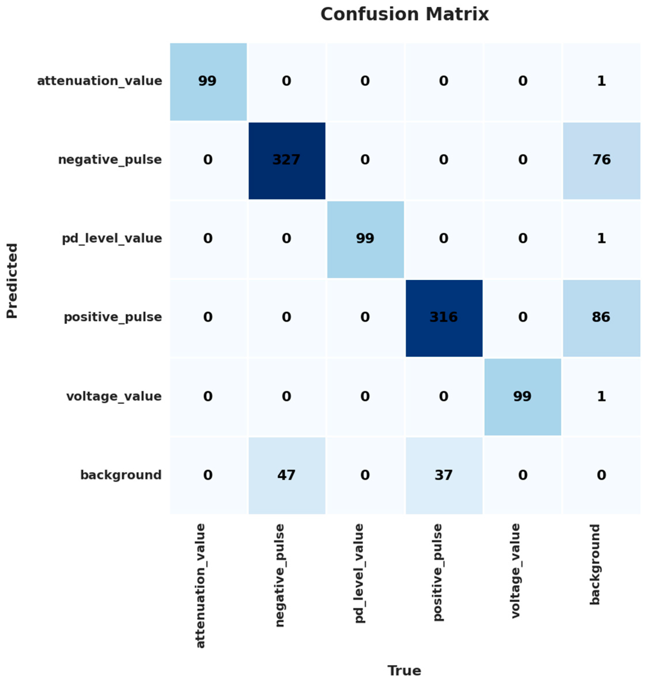
Figure 15.
Flowchart explaining how inference is performed from video sequences from the electrical sensor for object detection and quantitative data extraction.
Figure 15.
Flowchart explaining how inference is performed from video sequences from the electrical sensor for object detection and quantitative data extraction.
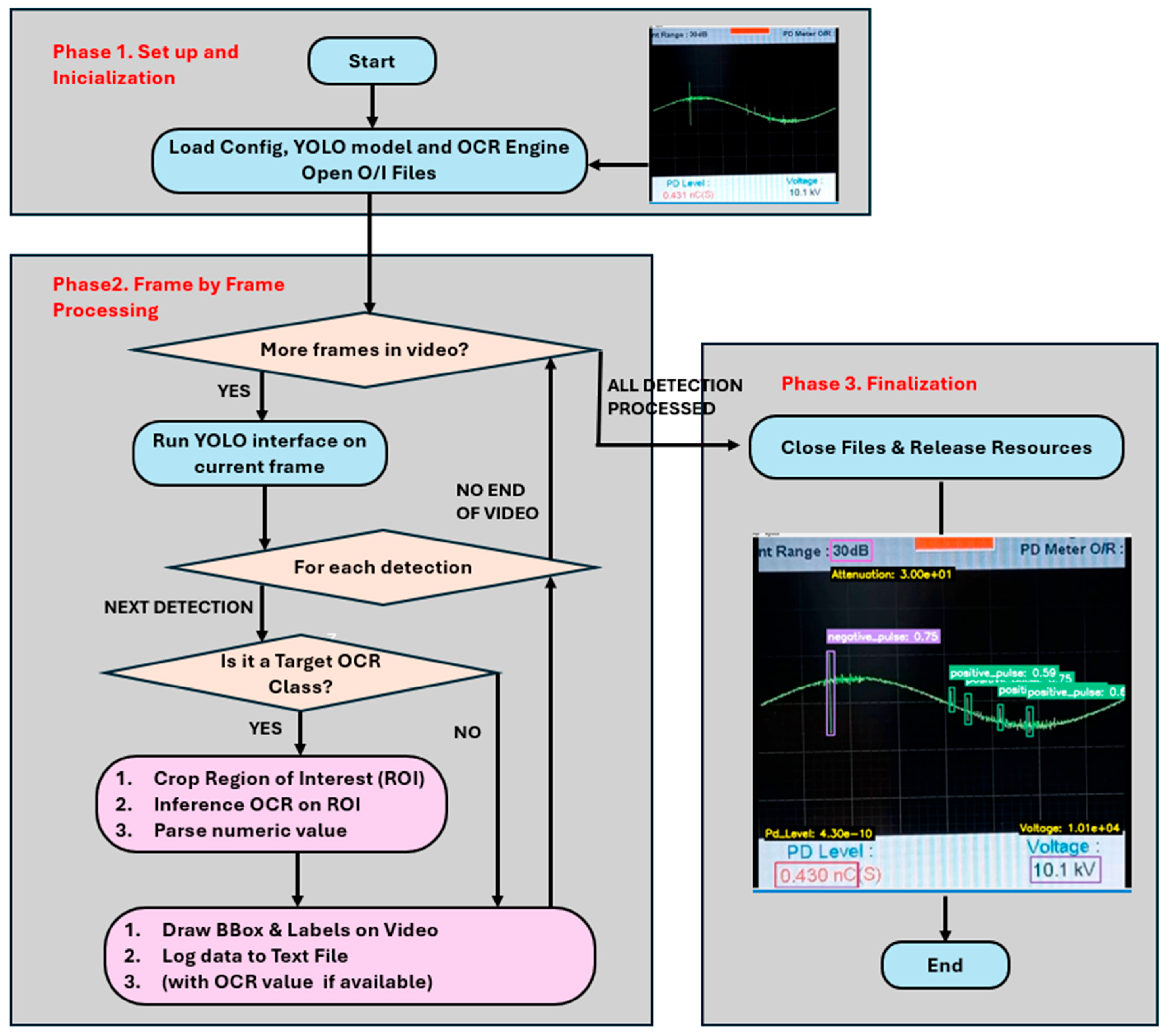
Figure 16.
Inference for 3 images from the trained CNN.
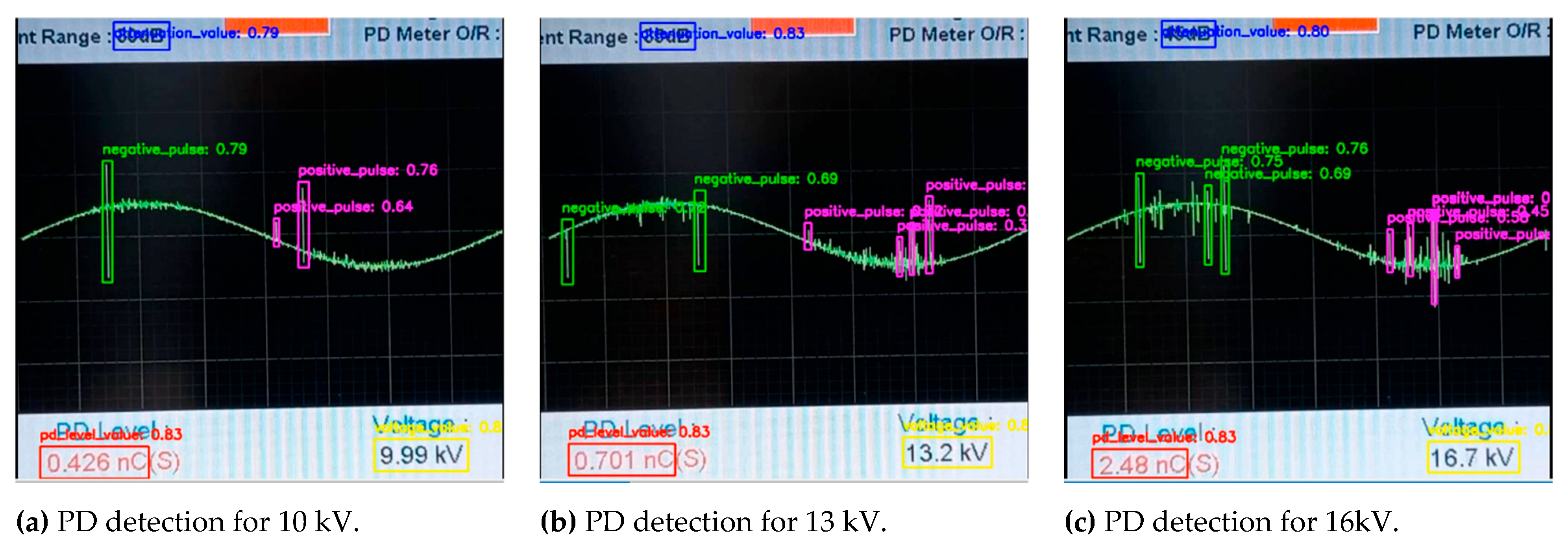
Figure 17.
Accumulated detection images for each PD video of 10 s duration.
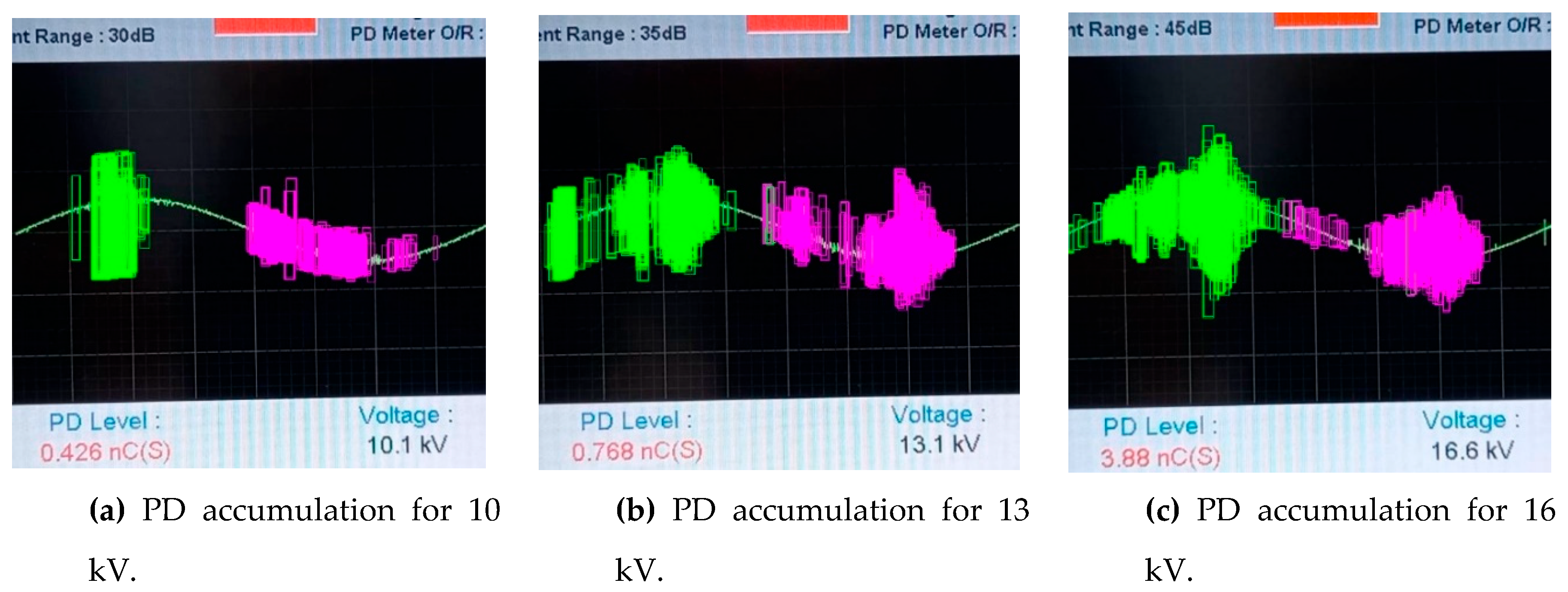
Figure 18.
High-level logical flow of the script focusing on the three main phases: configuration, processing and detection, and dataset generation.
Figure 18.
High-level logical flow of the script focusing on the three main phases: configuration, processing and detection, and dataset generation.
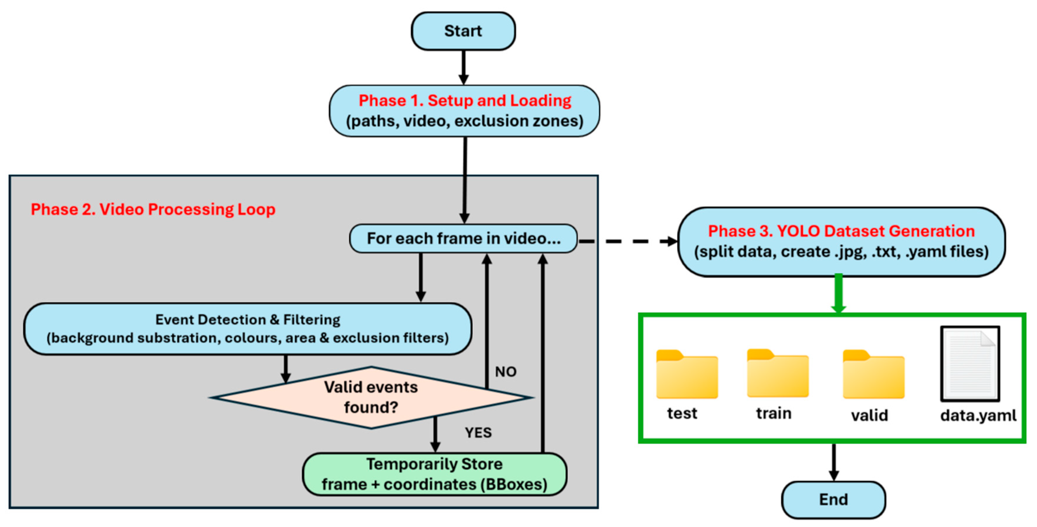
Figure 19.
Background and PDs with bounding boxes.
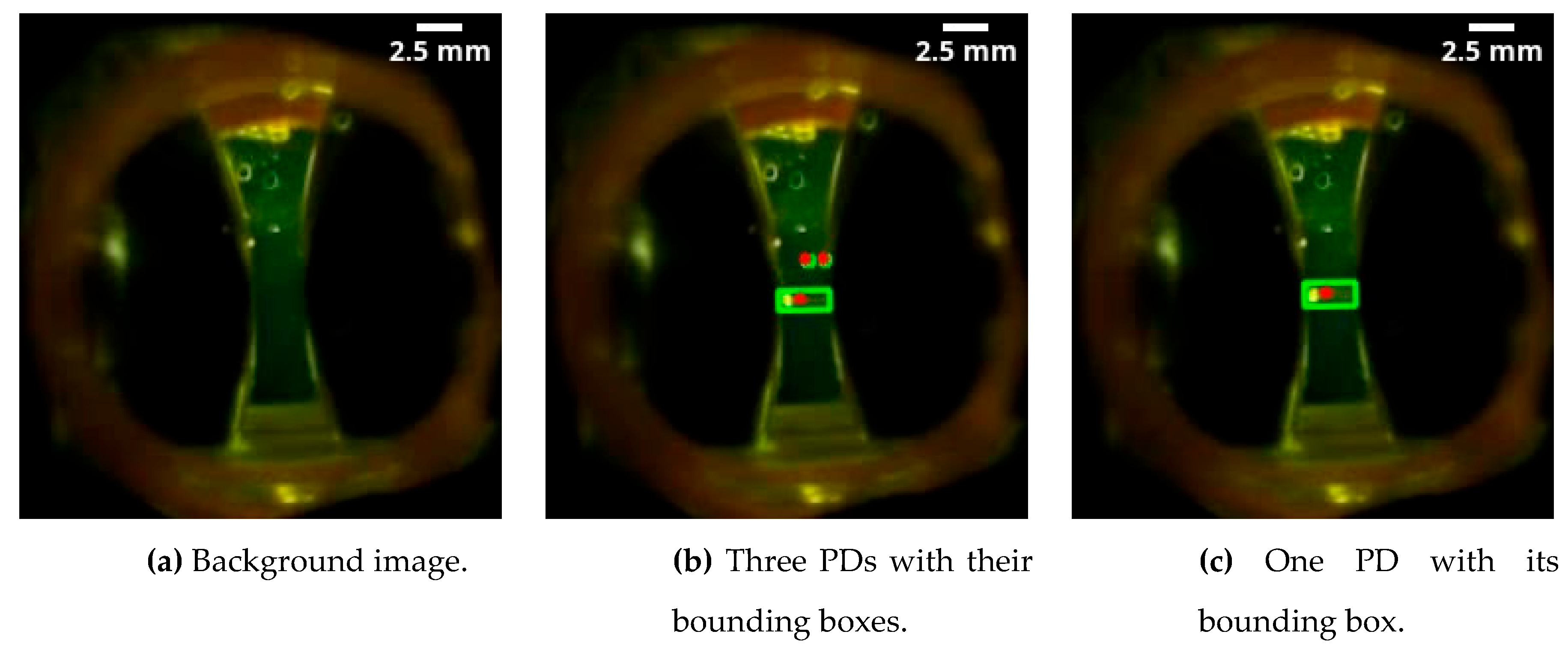
Figure 20.
Training vs Validation Box and Classification curves.
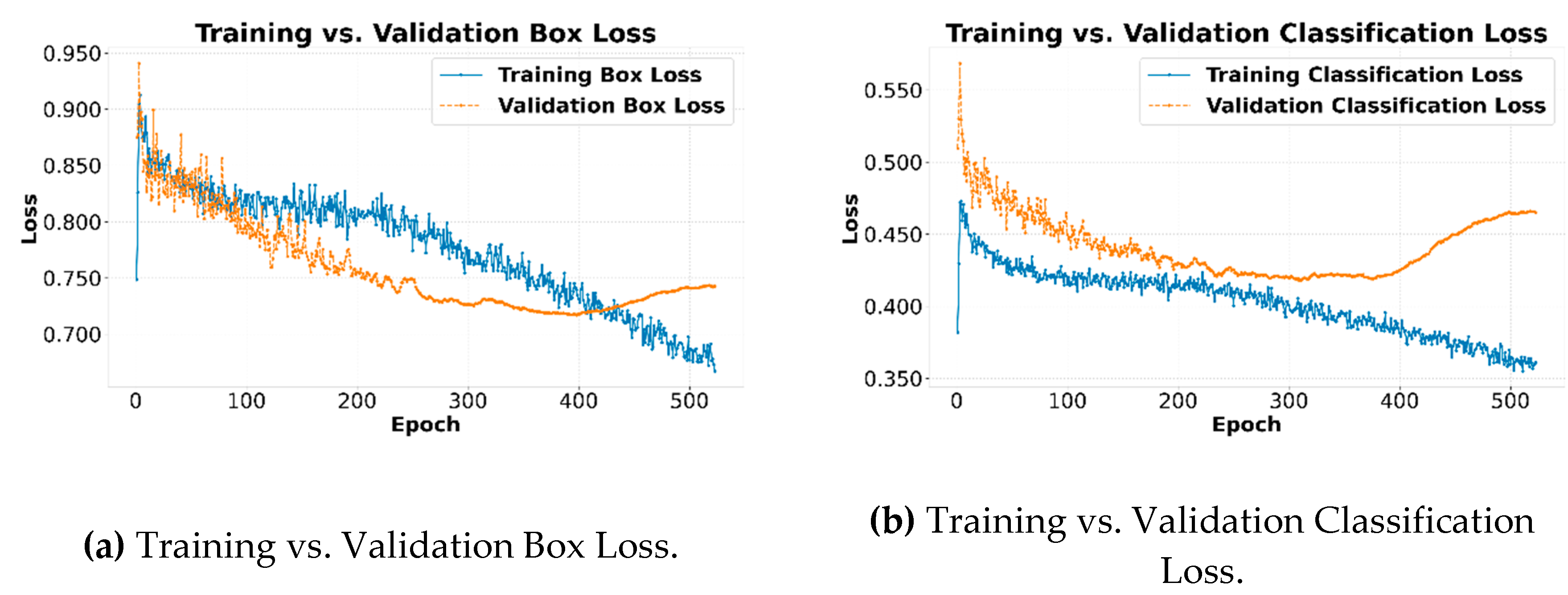
Figure 21.
Training vs Validation DFL Loss and Training Precision curves.
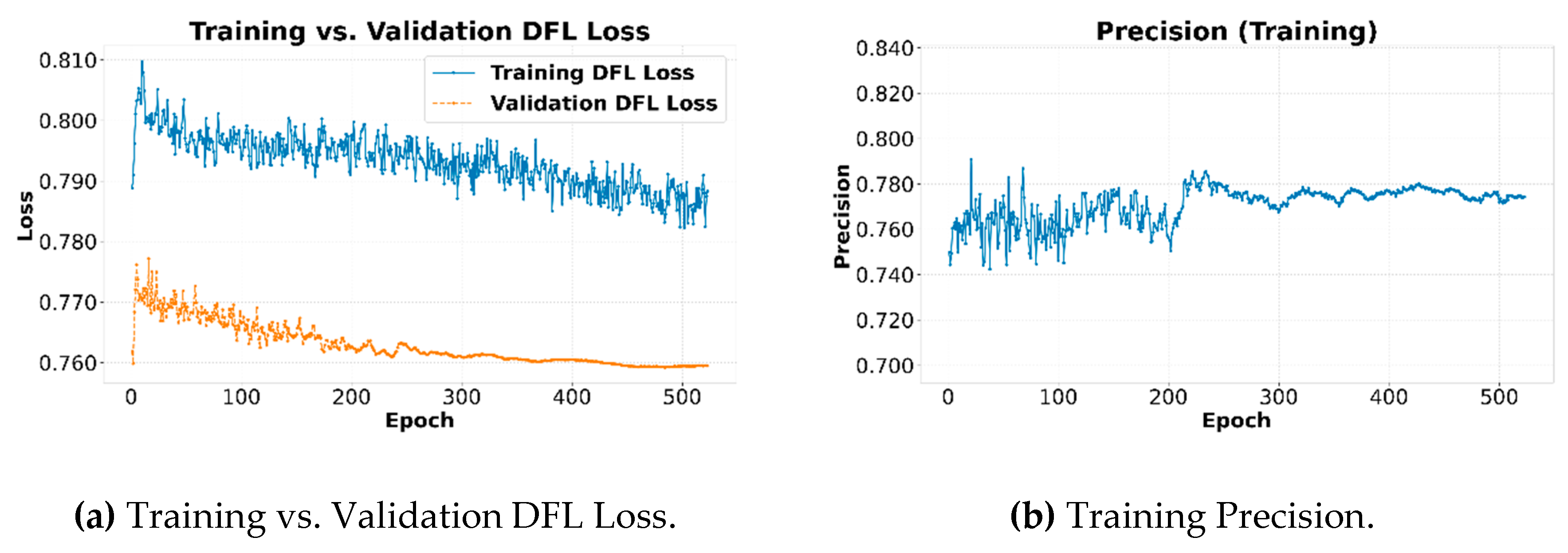
Figure 22.
PD inference and confidence estimated by CNN for 10 kV, 13 kV and 16 kV.
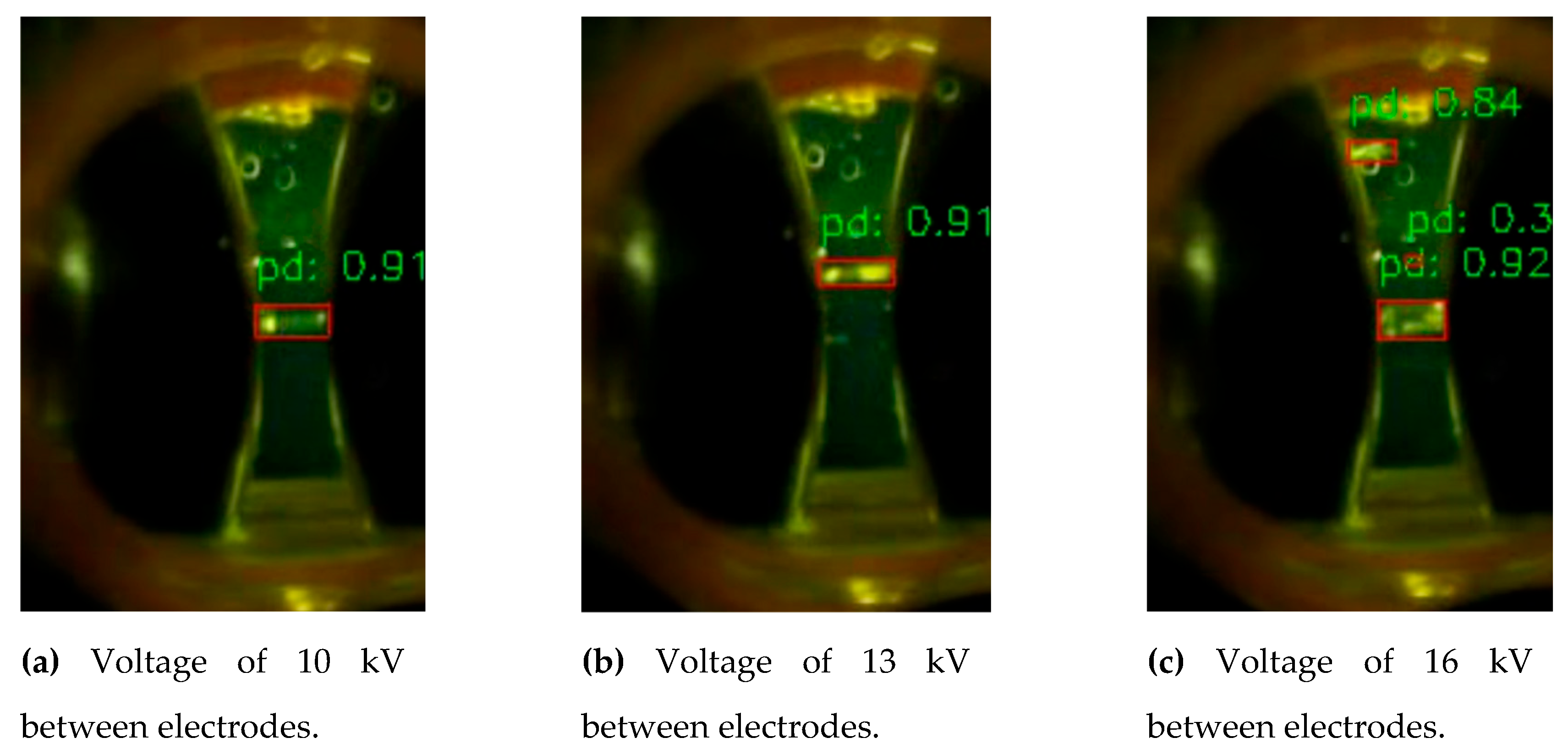
Figure 23.
Distribution of centers of PD inference estimated by CNN for 10 kV, 13 kV and 16 kV.
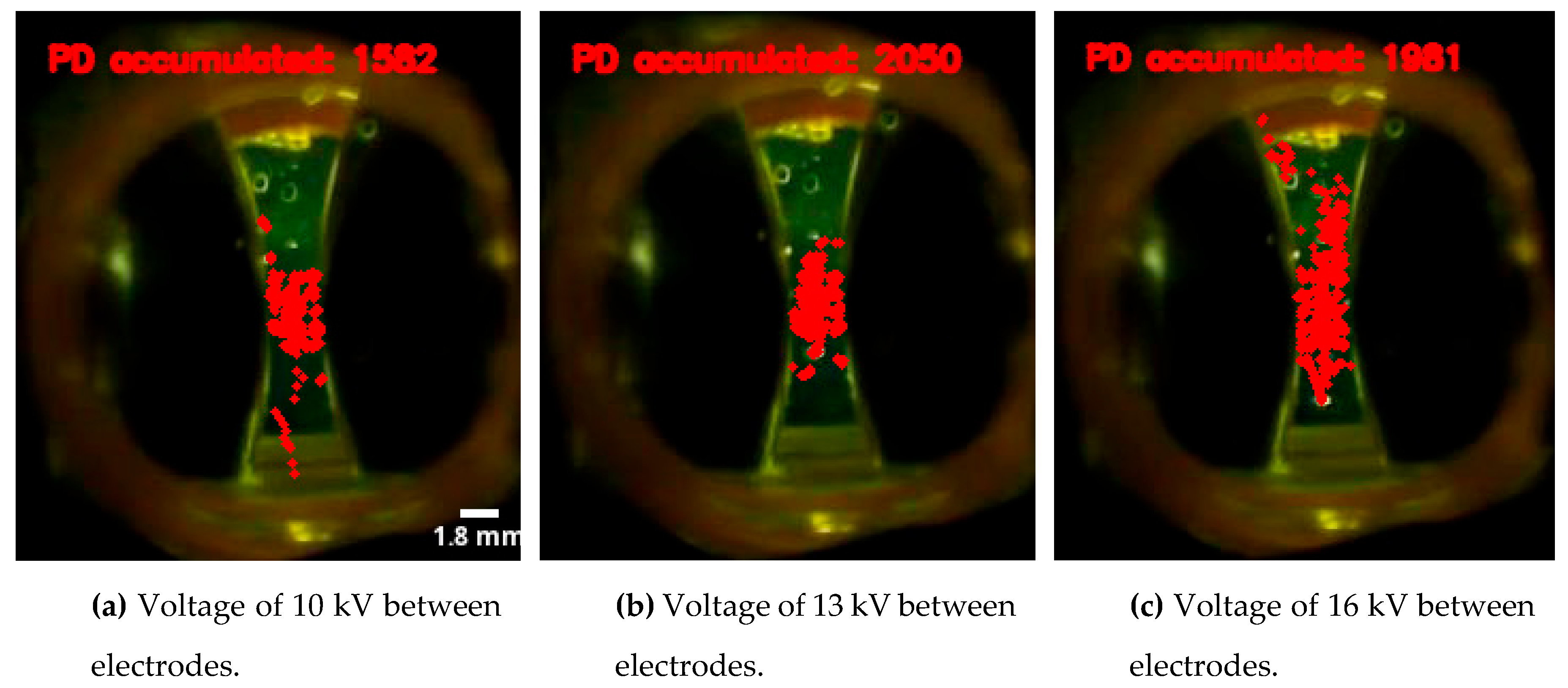
Figure 24.
Cumulative distribution of PD centers and magnitude of each associated box in pixels² and confidence of each point for 10 kV.
Figure 24.
Cumulative distribution of PD centers and magnitude of each associated box in pixels² and confidence of each point for 10 kV.
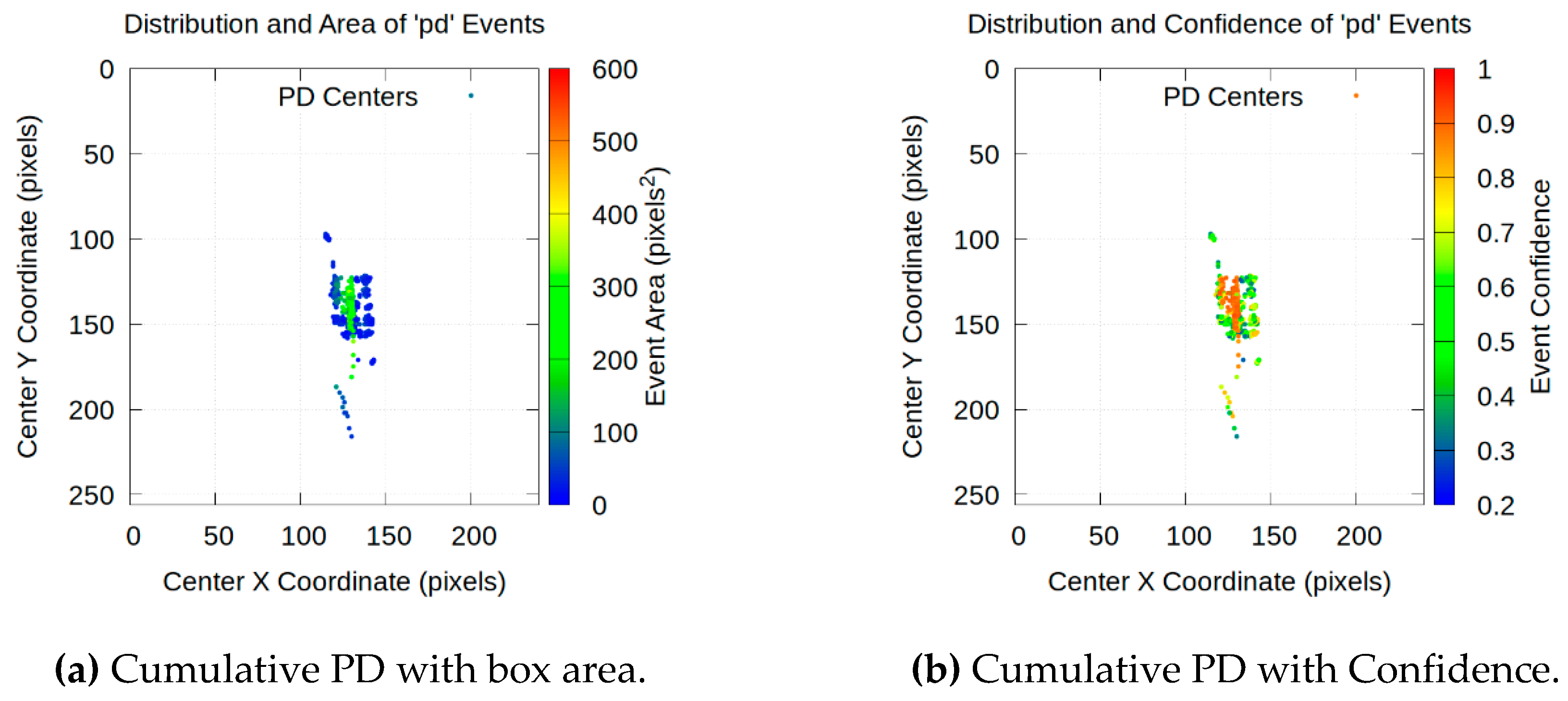
Figure 25.
Cumulative distribution of PD centers and magnitude of each associated box in pixels² and confidence of each point for 13 kV.
Figure 25.
Cumulative distribution of PD centers and magnitude of each associated box in pixels² and confidence of each point for 13 kV.
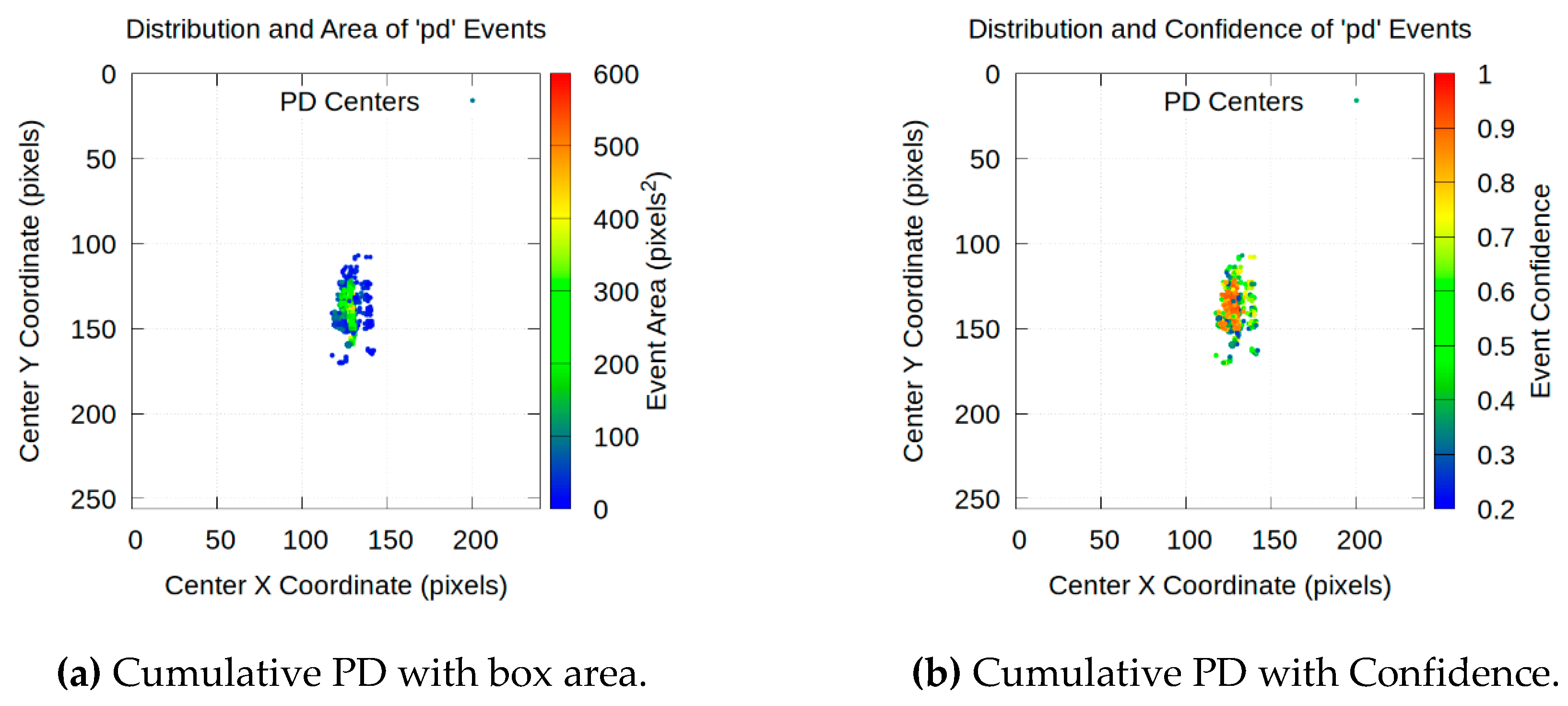
Figure 26.
Cumulative distribution of PD centers and magnitude of each associated box in pixels² and confidence of each point for 16 kV.
Figure 26.
Cumulative distribution of PD centers and magnitude of each associated box in pixels² and confidence of each point for 16 kV.
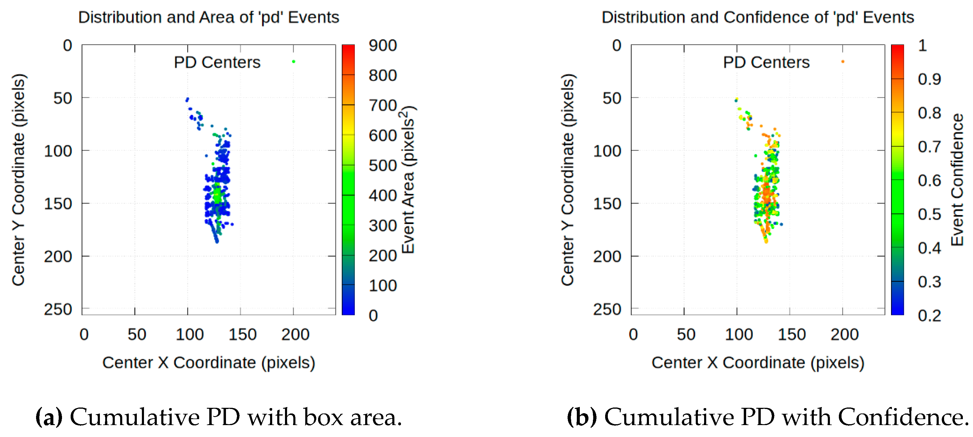

Table 1.
Summary of the most relevant Pearson correlation coefficients (r).
| Attribute 1 | Attribute 2 | Coefficient (r) |
|---|---|---|
| Strong positive correlations (r > 0.7) | ||
| ocr_voltage | ocr_pd_level | 0.90 |
| num_pulse_negatives | ocr_voltage | 0.77 |
| Area | Height | 0.90 |
| Area | Width | 0.78 |
| CenterX | CenterY | 0.77 |
| Significant negative correlations (r < -0.3) | ||
| ocr_voltage | Width | -0.41 |
| ocr_pd_level | Width | -0.39 |
| num_pulsos_negativos | Width | -0.34 |
| Other moderate positive correlations (0.5 < r < 0.7) | ||
| num_pulse_negatives | ocr_pd_level | 0.59 |
| Confidence | Width | 0.55 |
| Area | Confidence | 0.53 |
Disclaimer/Publisher’s Note: The statements, opinions and data contained in all publications are solely those of the individual author(s) and contributor(s) and not of MDPI and/or the editor(s). MDPI and/or the editor(s) disclaim responsibility for any injury to people or property resulting from any ideas, methods, instructions or products referred to in the content. |
© 2025 by the authors. Licensee MDPI, Basel, Switzerland. This article is an open access article distributed under the terms and conditions of the Creative Commons Attribution (CC BY) license (http://creativecommons.org/licenses/by/4.0/).
Copyright: This open access article is published under a Creative Commons CC BY 4.0 license, which permit the free download, distribution, and reuse, provided that the author and preprint are cited in any reuse.


