Submitted:
02 September 2025
Posted:
02 September 2025
You are already at the latest version
Abstract
We investigate the off-shell generalized parton distributions (GPDs) of kaons within the framework of the Nambu–Jona-Lasinio model, employing proper time regularization. In comparison to pion off-shell GPDs, the effects of off-shellness in kaons are found to be comparable. The influence of these off-shell effects on GPDs is approximately $10\%$ to $25\%$, which is significant. Additionally, the $x$-moments of off-shell GPDs exhibit odd powers due to a lack of crossing symmetry, leading to the emergence of new off-shell form factors. We explore the relationships among the off-shell form factors for kaons, drawing an analogy with their electromagnetic counterparts. Our findings extend pion off-shell GPDs to include those for kaons while simultaneously addressing their associated off-shell form factors. Furthermore, we examine and compare the off-shell gravitational form factors of kaons with their on-shell counterparts.
Keywords:
off-shell generalized parton distributions
; Nambu–Jona-Lasinio model
; off-shell form factors
1. Introduction
One of the most important topics in hadronic physics is understanding the internal structures of hadrons in terms of quarks and gluons. The partonic structure of a hadron is effectively characterized by various light-cone partonic distribution functions, such as parton distribution functions (PDFs) [1,2,3]. PDFs represent the diagonal matrix elements of specific operators and serve as essential inputs for theoretical calculations of physical observables in deep inelastic scattering (DIS) high-energy processes. However, PDFs only describe the longitudinal momentum distribution of partons within hadrons. To gain insight into the three-dimensional internal structure of a hadron, one must consider non-diagonal or off-forward matrix elements. These non-diagonal matrix elements can be parameterized using generalized parton distributions (GPDs) [4,5,6,7,8,9,10,11,12,13,14,15,16,17,18,19].
Since their proposal, GPDs have been extensively studied because they elucidate the partonic probability densities concerning longitudinal momentum, transverse position, and angular momentum. This means that GPDs contain information about how partons are distributed in a plane perpendicular to the direction of motion of the hadron. Consequently, one can derive the three-dimensional structure of hadrons through GPDs. On one hand, different Mellin moments of GPDs are associated with various hadron form factors (FFs) [20,21,22,23], including electromagnetic FFs [24], axial FFs, gravitational FFs (GFFs), and transition FFs [25]. The GFFs are linked to the energy-momentum tensor [26], which facilitates a gauge-invariant spin decomposition of hadrons. Furthermore, these distributions encompass mass and pressure profiles as well as their Fourier transforms related to Breit-frame pressure distributions and shear pressure distributions. On the other hand, in the forward limit, GPDs reduce to conventional PDFs. For GPDs at zero skewness, by performing a Fourier transform on the transverse component of momentum transfer, one can derive the impact parameter distribution (IPD). The IPD elucidates the probability density of locating a parton at a transverse distance from the center of momentum of the hadron with longitudinal momentum fraction x. In general, GPDs contain substantial information regarding angular momentum, mass, and mechanical properties of hadrons. They provide critical insights into spatial distributions as well as spin and orbital motion of quarks within these particles.
These features render GPDs a crucial component in various types of hard exclusive and elastic scattering processes, including deeply virtual Compton scattering (DVCS) [27,28,29,30], deep virtual meson production (DVMP) [31,32,33], and timelike Compton scattering (TCS) [34,35,36,37,38]. Through these experimental processes, researchers gain valuable insights into GPDs. Recently, GPDs have been extracted by analyzing global electron scattering data [39,40].
The phenomenological determination of GPDs is less advanced than the contemporary analyses of PDFs and FFs. However, interest in GPDs is rapidly increasing due to the recent approval of the U.S. Electron-Ion Collider (EIC) and the electron-ion colliders in China (EicC). Additionally, lattice QCD has made first-principle calculations of GPDs more accessible.
The studies presented in Refs. [41,42] investigate the accessibility of pion GPDs through the Sullivan process [43] at future electron-ion colliders. They conclude that experimental access may soon be feasible. The amplitude associated with the Sullivan process involves an off-shell pion, necessitating careful consideration of potential off-shellness issues both within the process and in the GPDs themselves.
In addition, transverse momentum dependent parton distributions (TMDs) [44,45] provide a more comprehensive understanding of parton structures, particularly the transverse characteristics of hadrons. Therefore, we also compute the off-shell TMDs for kaons.
In Refs. [46,47,48], investigations into the off-shell behavior of pion GPDs are conducted using a chiral quark model. In this paper, we extend our analysis from pion off-shell GPDs to kaon off-shell GPDs within the framework of the Nambu–Jona-Lasinio (NJL) model [49,50,51,52,53]. The NJL model incorporates global symmetries inherent to Quantum Chromodynamics (QCD), particularly emphasizing chiral symmetry. In this effective model, gluonic degrees of freedom have been integrated out, resulting in point-like interactions between quarks; however, this characteristic renders the NJL model non-renormalizable. Consequently, it is imperative to select an appropriate regularization scheme to fully define this model. The NJL framework has been extensively employed for studying hadronic structure [54,55,56,57,58,59,60,61,62,63,64,65,66].
This paper is organized as follows: In Section 2, we provide a concise introduction to the NJL model, followed by the definition and calculation of kaon off-shell GPDs. Additionally, we will examine the fundamental properties of off-shell kaon GPDs in this section. In Section 3, the off-shell TMDs of the kaon are evaluated. In Section 4, we present a brief summary and outlook.
2. The Off-Shell GPDs
2.1. Nambu–Jona-Lasinio Model
The SU(3) flavor NJL Lagrangian in the interaction channel is presented in the form described in [67],
The quark field is represented by the flavor components . The matrices , where , denote the eight Gell-Mann matrices in flavor space. Notably, is defined as . The current quark mass matrix is represented as . The parameter denotes the effective coupling strength associated with the scalar interaction channel () and the pseudoscalar interaction channel ().
The dressed quark propagator within the framework of the NJL model is derived by solving the gap equation illustrated in Figure 1
the dressed quark mass is denoted as . The interaction kernel of the gap equation illustrated in Fig. Figure 1 is local; therefore, we obtain a constant dressed quark mass , which satisfies the following condition:
the trace is taken over Dirac indices. From the preceding equation, it is evident that the SU(3) flavor case contrasts with the SU(2) flavor scenario, as flavor mixing is absent [49,68]. Furthermore, dynamical chiral symmetry breaking can occur only when the coupling constant , which yields a nontrivial solution where .
In the NJL model, mesons are described as bound states of , which is derived from the Bethe-Salpeter equation (BSE). The solution to the BSE in each meson channel is represented by a two-body t-matrix that varies according to the specific nature of the interaction channel. For instance, the reduced t-matrices for kaon mesons can be expressed as follows:
the bubble diagram is defined as
the traces are taken over Dirac and isospin indices. The mass of the kaon is determined by the pole in the reduced t-matrix
Expanding the complete t-matrix around the pole yields the homogeneous Bethe-Salpeter vertex for the kaon
the normalization factor is defined as follows:
This residue can be interpreted as the square of the effective meson-quark-quark coupling constant. Homogeneous Bethe-Salpeter vertex functions are essential components in, for instance, triangle diagrams that determine the form factors of mesons.
The NJL model is a non-renormalizable framework, necessitating the implementation of a regularization scheme. In this context, we will employ the PTR scheme [69,70,71].
The expression X denotes a product of propagators that have been interconnected through Feynman parametrization. The symbol represents the ultraviolet cutoff. It is important to note that the NJL model does not incorporate confinement; thus, an infrared cutoff is employed to simulate this effect. Consequently, it should be on the order of . For our purposes, we select GeV.
For the dressed masses of light quarks, we select GeV, the strange quark mass GeV. The ultraviolet cutoff and the coupling constant are constrained by empirical values for the pion decay constant and pion mass. The kaon is treated as a relativistic bound state composed of a dressed quark and a dressed antiquark, with its properties determined by solving the Bethe-Salpeter equation in the pseudoscalar channel for the system. In Table 1, we present the parameters utilized in this study.
In the subsequent sections, we will employ the functions and formulas as detailed in the appendix.
2.2. The Off-Shell Kaon GPDs
In the NJL model, the kaon off-shell GPDs are illustrated in Figure 2. Here, p represents the initial kaon momentum, while denotes the final kaon momentum. In the case of off-shell conditions where , the kinematics and related quantities pertinent to this process are defined as follows:
where represents the skewness parameter, and n denotes the light-cone four-vector defined as in the context of light-cone coordinates
for any four-vector , it can be defined in light-cone coordinates as follows:
The vector and tensor quark GPDs of kaon are defined as
where x represents the longitudinal momentum fraction. The function denotes the non-spin-flip or vector GPD, while corresponds to the spin-flip or tensor GPD.
The operators depicted in Figure 2 for off-shell kaon GPDs are structured as follows:
where the first for vector GPD and the second for tensor GPD.
In the NJL model, the vector and tensor GPDs of the u quark in the meson are defined as follows:
where , , .
Here we use the notations
one can derive the following simplified formulas
after some calculation we arrive at
and
We denote the step function by . It takes the value of 1 in the corresponding region, and is otherwise equal to zero. These results pertain to the region where . Under the transformation , we observe that: ; furthermore, both and remain invariant.
The diagrams of and are presented in Figure 3 and Figure 4. The off-shellness is influenced by at the condition where . The diagrams illustrate that as increases, the off-shell effects of half-off-shell pion GPDs become increasingly pronounced. Specifically, at , this relative effect reaches approximately , while at , it escalates to about . These findings are consistent with those observed for off-shell pion GPDs.
2.3. The Properties of Kaon Off-Shell GPDs
2.3.1. Forward Limit
In the case the initial and final kaon have the same momentum , which means , , vector GPD reduces to kaon PDF,
when the skewness parameter , the function vanishes in the region where . In contrast, for the region where , this off-shell PDF of the u quark in kaons differs from that of pions as described in the NJL model [12,72].
In Figure 5, we present the diagram of the off-shell u quark PDF. It is evident that when and , the lines are nearly straight. As increases, particularly in the context of an off-shell kaon, a more pronounced dependence on x emerges. The NJL model effectively describes low-energy properties within QCD. At high values of , however, evolution becomes necessary; consequently, the dependence on x will vary as a result of this evolution. Different from the pion PDF, the position of x corresponding to the maximum value of the function has shifted to a region where x is less than .
2.3.2. Polynomiality Condition
The x-moments of the off-shell GPDs also include odd powers of the skewness parameter .
When , we obtain FFs
where and are the u quark vector and tensor FFs. and are FFs due to the off-shellness. and are symmetry about the p and , but and are antisymmetry about p and .
The functions and are defined in the general covariant structure of the kaon-photon vertex:
at , the relationship [48]
where indicates that, due to crossing symmetry, one can conclude that . Here, represents the electromagnetic FFs, and it is noted that . From the off-shell kaon GPDs, one can derive
where .
We demonstrate that our is equivalent to as presented in Eq. (28), consistent with the findings of Ref. [48].
For , GPDs should follow the sum rule:
where pertains to the mass distribution of the u quark within the kaon, while is associated with the pressure distribution of the u quark. The polynomial contains only the terms and , thereby satisfying Eqs. (Section 2.3.2). The generalized FFs for are as follows:
For the u quark tensor GPD of the kaon within the NJL model, it is noted that .
2.3.3. Impact Parameter Denpendent PDFs
The impact parameter dependent PDFs are given by,
This means that the impact parameter dependent PDFs defined above are the Fourier transform of , therefore, when we obtain , parton distribution as a function of the distance and the light-cone momentum fraction x can be determined.
When and , GPDs become
where x is defined within the interval , we can derive the following:
when integrating , we can obtain the u quark PDF as presented in Eq. (24).
Figure 6 illustrates the off-shell impact parameter space PDFs multiplied by x at GeV−2 for various values of . From the diagram, it is evident that the maximum value of corresponds to a larger value of x compared to that associated with the maximum value of . As the value of increases, the maximum values of and also rise. Concurrently, with the increase in , the position x that corresponds to the maximum value of decreases, while maintaining a coordinate where . In contrast, for , as increases, the position of x corresponding to its maximum values remains relatively unchanged, hovering around approximately .
3. The Kaon Off-Shell TMDs
The kaon TMD is depicted in Figure 7. Within the context of the Nambu-Jona-Lasinio (NJL) model, it is defined as follows:
where represents a trace over spinor indices. As a result, we have successfully derived the final expression for the off-shell kaon TMD.
in Figure 8, we plot a three-dimensional diagram of the on-shell and off-shell kaon TMD at GeV2. For the on-shell case, it is evident that as , the function reaches its maximum value. This behavior contrasts with that of the pion on-shell TMD. The off-shell TMD exhibits a more pronounced dependence on x, resembling the characteristics of the pion off-shell TMD. However, it is noteworthy that the value of x corresponding to the maximum has shifted to a position less than , which distinguishes it from both the pion on-shell and off-shell TMDs, as those are symmetric about . The off-shell kaon PDF as articulated in Eq. (24) can be derived through the integration over .
4. Summary and Outlook
In this paper, we investigate the off-shell generalized parton distributions (GPDs) and transverse momentum dependent parton distributions (TMDs) of kaons within the framework of the Nambu–Jona-Lasinio (NJL) model, employing proper time regularization. We derive off-shell form factors (FFs), off-shell parton distribution functions (PDFs), and impact parameter-dependent PDFs. Subsequently, we compare these distributions with their on-shell counterparts and examine their properties.
Unlike on-shell GPDs, the lack of crossing symmetry in off-shell GPDs results in their Mellin moments exhibiting not only even powers of the skewness parameter but also odd powers. This indicates the emergence of new off-shell FFs. Our findings indicate the modifications in kaon GPDs resulting from off-shell effects. Unlike their on-shell counterparts, certain properties may not hold in the off-shell scenario; for instance, symmetry properties and polynomiality conditions may no longer be applicable.
For the off-shell kaon GPDs, the relative off-shell effect ranges from approximately to . We have also conducted a comparison between the off-shell kaon GPDs and those of pions. By analyzing the Mellin moments of kaon GPDs, we derive both the off-shell FFs and gravitational FFs. Furthermore, we compare the off-shell FFs of kaons with those of pions.
In summary, the NJL model has been demonstrated to effectively describe the off-shell characteristics of pion and kaon structures. In future work, we can extend these calculations to encompass the off-shell GPDs and FFs of vector mesons such as and , as well as protons and neutrons. Furthermore, we can replicate the results for off-shell GPDs obtained in this study using models that incorporate more realistic interactions; this may provide additional insights into the underlying physics.
Acknowledgments
Work supported by: the Scientific Research Foundation of Nanjing Institute of Technology (Grant No. YKJ202352).
Appendix A. Useful Formulae
Here we use the gamma-functions (, )
where are, respectively, the infrared and ultraviolet regulators described above.
The functions denoted by are defined as follows:
References
- Z.-N. Xu, author D. Binosi, author C. Chen, author K. Raya, author C. D. Roberts, and author J. Rodríguez-Quintero, Phys. Lett. B volume 865, pages 139451 ( year 2025), http://arxiv.org/abs/2411.15376 arXiv:2411.15376 [hep-ph] NoStop.
- Q. Wu, author Z.-F. Cui, and author J. Segovia, Phys. Rev. D volume 111, pages 116023 ( year 2025), http://arxiv.org/abs/2503.07055 arXiv:2503.07055 [hep-ph] NoStop.
- Tanisha, author S. Puhan, author A. Yadav, and author H. Dahiya, ( year 2025), http://arxiv.org/abs/2505.09213 arXiv:2505.09213 [hep-ph] NoStop.
- D. Muller, author D. Robaschik, author B. Geyer, author F. M. Dittes, and author J. Horejsi, Fortsch. Phys. volume 42, pages 101 ( year 1994), http://arxiv.org/abs/hep-ph/9812448 arXiv:hep-ph/9812448 [hep-ph] NoStop.
- X.-D. Ji, Phys. Rev. D volume 55, pages 7114 ( year 1997), http://arxiv.org/abs/hep-ph/9609381 arXiv:hep-ph/9609381 NoStop.
- A. V. Radyushkin, Phys. Rev. D volume 56, pages 5524 ( year 1997), http://arxiv.org/abs/hep-ph/9704207 arXiv:hep-ph/9704207 NoStop.
- X.-D. Ji, J. Phys. G volume 24, pages 1181 ( year 1998), http://arxiv.org/abs/hep-ph/9807358 arXiv:hep-ph/9807358 NoStop.
- L. Theussl, author S. Noguera, and author V. Vento, Eur. Phys. J. A volume 20, pages 483 ( year 2004), http://arxiv.org/abs/nucl-th/0211036 arXiv:nucl-th/0211036 NoStop.
- M. Diehl, Phys. Rept. volume 388, pages 41 ( year 2003), http://arxiv.org/abs/hep-ph/0307382 arXiv:hep-ph/0307382 NoStop.
- J.-L. Zhang, author Z.-F. Cui, author J. Ping, and author C. D. Roberts, Eur. Phys. J. C volume 81, pages 6 ( year 2021), http://arxiv.org/abs/2009.11384 arXiv:2009.11384 [hep-ph] NoStop.
- J.-L. Zhang, author K. Raya, author L. Chang, author Z.-F. Cui, author J. M. Morgado, author C. D. Roberts, and author J. Rodríguez-Quintero, Phys. Lett. B volume 815, pages 136158 ( year 2021), http://arxiv.org/abs/2101.12286 arXiv:2101.12286 [hep-ph] NoStop.
- J.-L. Zhang, author M.-Y. Lai, author H.-S. Zong, and author J.-L. Ping, Nucl. Phys. B volume 966, pages 115387 ( year 2021) NoStop.
- J.-L. Zhang and author J.-L. Ping, Eur. Phys. J. C volume 81, pages 814 ( year 2021) NoStop.
- J.-L. Zhang, author G.-Z. Kang, and author J.-L. Ping, Chin. Phys. C volume 46, pages 063105 ( year 2022), http://arxiv.org/abs/2110.06463 arXiv:2110.06463 [hep-ph] NoStop.
- J.-L. Zhang, author G.-Z. Kang, and author J.-L. Ping, Phys. Rev. D volume 105, pages 094015 ( year 2022), http://arxiv.org/abs/2204.14032 arXiv:2204.14032 [hep-ph] NoStop.
- C. Mezrag, Few Body Syst. volume 63, pages 62 ( year 2022), http://arxiv.org/abs/2207.13584 arXiv:2207.13584 [hep-ph] NoStop.
- J.-W. Qiu and author Z. Yu, JHEP volume 08, pages 103 ( year 2022), http://arxiv.org/abs/2205.07846 arXiv:2205.07846 [hep-ph] NoStop.
- J.-L. Zhang, ( year 2024), http://arxiv.org/abs/2409.04105 arXiv:2409.04105 [hep-ph] NoStop.
- M. Goharipour, author M. H. Amiri, author F. Irani, author H. Hashamipour, and author K. Azizi ( collaboration MMGPDs), ( year 2025), http://arxiv.org/abs/2508.15073 arXiv:2508.15073 [hep-ph] NoStop.
- J.-L. Zhang, Chin. Phys. C volume 49, pages 043104 ( year 2025), http://arxiv.org/abs/2409.19525 arXiv:2409.19525 [hep-ph] NoStop.
- S. Bondarenko and author M. Slautin, ( year 2025), http://arxiv.org/abs/2506.22153 arXiv:2506.22153 [hep-ph] NoStop.
- R. J. Hernández-Pinto, author L. X. Gutiérrez-Guerrero, author M. A. Bedolla, and author A. Bashir, Phys. Rev. D volume 110, pages 114015 ( year 2024), http://arxiv.org/abs/2410.23813 arXiv:2410.23813 [hep-ph] NoStop.
- S. Puhan and author H. Dahiya, Phys. Rev. D volume 111, pages 114039 ( year 2025), http://arxiv.org/abs/2505.02507 arXiv:2505.02507 [hep-ph] NoStop.
- P. Cheng, author Z.-Q. Yao, author D. Binosi, and author C. D. Roberts, Phys. Lett. B volume 862, pages 139323 ( year 2025), http://arxiv.org/abs/2412.10598 arXiv:2412.10598 [hep-ph] NoStop.
- J.-L. Zhang and author J. Wu, Chin. Phys. C volume 48, pages 083106 ( year 2024), http://arxiv.org/abs/2402.12757 arXiv:2402.12757 [hep-ph] NoStop.
- X. Ji and author C. Yang, ( year 2025), http://arxiv.org/abs/2508.16727 arXiv:2508.16727 [hep-ph] NoStop.
- K. Goeke, author M. V. Polyakov, and author M. Vanderhaeghen, Prog. Part. Nucl. Phys. volume 47, pages 401 ( year 2001), http://arxiv.org/abs/hep-ph/0106012 arXiv:hep-ph/0106012 NoStop.
- A. V. Radyushkin, Phys. Lett. B volume 380, pages 417 ( year 1996), http://arxiv.org/abs/hep-ph/9604317 arXiv:hep-ph/9604317 NoStop.
- A. Hobart ( collaboration CLAS), EPJ Web Conf. volume 290, pages 06001 ( year 2023) NoStop.
- G. Xie, author W. Kou, author Q. Fu, author Z. Ye, and author X. Chen, Eur. Phys. J. C volume 83, pages 900 ( year 2023), http://arxiv.org/abs/2306.02357 arXiv:2306.02357 [hep-ph] NoStop.
- D. Müller, author T. Lautenschlager, author K. Passek-Kumericki, and author A. Schaefer, Nucl. Phys. B volume 884, pages 438 ( year 2014), http://arxiv.org/abs/1310.5394 arXiv:1310.5394 [hep-ph] NoStop.
- L. Favart, author M. Guidal, author T. Horn, and author P. Kroll, Eur. Phys. J. A volume 52, pages 158 ( year 2016), http://arxiv.org/abs/1511.04535 arXiv:1511.04535 [hep-ph] NoStop.
- M. Čuić, author G. Duplančić, author K. Kumerički, and author K. Passek-K., JHEP volume 12, pages 192 ( year 2023), note [Erratum: JHEP 02, 225 (2024)], http://arxiv.org/abs/2310.13837 arXiv:2310.13837 [hep-ph] NoStop.
- E. R. Berger, author M. Diehl, and author B. Pire, Eur. Phys. J. C volume 23, pages 675 ( year 2002), http://arxiv.org/abs/hep-ph/0110062 arXiv:hep-ph/0110062 NoStop.
- M. Boër, author M. Guidal, and author M. Vanderhaeghen, Eur. Phys. J. A volume 51, pages 103 ( year 2015) NoStop.
- Y.-P. Xie and author V. P. Goncalves, Phys. Lett. B volume 839, pages 137762 ( year 2023), http://arxiv.org/abs/2212.07657 arXiv:2212.07657 [hep-ph] NoStop.
- P. Chatagnon et al. ( collaboration CLAS), Phys. Rev. Lett. volume 127, pages 262501 ( year 2021), http://arxiv.org/abs/2108.11746 arXiv:2108.11746 [hep-ex] NoStop.
- G. M. Peccini, author L. S. Moriggi, and author M. V. T. Machado, Phys. Rev. D volume 103, pages 054009 ( year 2021), http://arxiv.org/abs/2101.08338 arXiv:2101.08338 [hep-ph] NoStop.
- H. Hashamipour, author M. Goharipour, author K. Azizi, and author S. V. Goloskokov, Phys. Rev. D volume 105, pages 054002 ( year 2022), http://arxiv.org/abs/2111.02030 arXiv:2111.02030 [hep-ph] NoStop.
- H. Hashamipour, author M. Goharipour, and author S. S. Gousheh, Phys. Rev. D volume 102, pages 096014 ( year 2020), http://arxiv.org/abs/2006.05760 arXiv:2006.05760 [hep-ph] NoStop.
- A. C. Aguilar et al., Eur. Phys. J. A volume 55, pages 190 ( year 2019), http://arxiv.org/abs/1907.08218 arXiv:1907.08218 [nucl-ex] NoStop.
- J. M. M. Chávez, author V. Bertone, author F. De Soto Borrero, author M. Defurne, author C. Mezrag, author H. Moutarde, author J. Rodríguez-Quintero, and author J. Segovia, Phys. Rev. Lett. volume 128, pages 202501 ( year 2022), http://arxiv.org/abs/2110.09462 arXiv:2110.09462 [hep-ph] NoStop.
- J. D. Sullivan, Phys. Rev. D volume 5, pages 1732 ( year 1972) NoStop.
- J.-L. Zhang and author J. Wu, Eur. Phys. J. C volume 85, pages 13 ( year 2025), http://arxiv.org/abs/2408.13569 arXiv:2408.13569 [hep-ph] NoStop.
- W.-Y. Liu and author I. Zahed, ( year 2025), http://arxiv.org/abs/2503.11959 arXiv:2503.11959 [hep-ph] NoStop.
- V. Shastry, author W. Broniowski, and author E. Ruiz Arriola, Phys. Rev. D volume 108, pages 114024 ( year 2023), http://arxiv.org/abs/2308.09236 arXiv:2308.09236 [hep-ph] NoStop.
- W. Broniowski, author V. Shastry, and author E. Ruiz Arriola, Acta Phys. Polon. Supp. volume 16, pages 7 ( year 2023), http://arxiv.org/abs/2304.02097 arXiv:2304.02097 [hep-ph] NoStop.
- W. Broniowski, author V. Shastry, and author E. Ruiz Arriola, Phys. Lett. B volume 840, pages 137872 ( year 2023), http://arxiv.org/abs/2211.11067 arXiv:2211.11067 [hep-ph] NoStop.
- S. P. Klevansky, Rev. Mod. Phys. volume 64, pages 649 ( year 1992) NoStop.
- M. Buballa, Phys. Rept. volume 407, pages 205 ( year 2005), http://arxiv.org/abs/hep-ph/0402234 arXiv:hep-ph/0402234 NoStop.
- J.-L. Zhang, author C.-M. Li, and author H.-S. Zong, Chin. Phys. C volume 42, pages 123105 ( year 2018) NoStop.
- J.-L. Zhang, author Y.-M. Shi, author S.-S. Xu, and author H.-S. Zong, Mod. Phys. Lett. A volume 31, pages 1650086 ( year 2016) NoStop.
- Z.-F. Cui, author I. C. Cloet, author Y. Lu, author C. D. Roberts, author S. M. Schmidt, author S.-S. Xu, and author H.-S. Zong, Phys. Rev. D volume 94, pages 071503 ( year 2016), http://arxiv.org/abs/1604.08454 arXiv:1604.08454 [nucl-th] NoStop.
- W. Bentz, author T. Hama, author T. Matsuki, and author K. Yazaki, Nucl. Phys. A volume 651, pages 143 ( year 1999), http://arxiv.org/abs/hep-ph/9901377 arXiv:hep-ph/9901377 NoStop.
- S. Noguera and author S. Scopetta, JHEP volume 11, pages 102 ( year 2015), http://arxiv.org/abs/1508.01061 arXiv:1508.01061 [hep-ph] NoStop.
- M. E. Carrillo-Serrano, author W. Bentz, author I. C. Cloët, and author A. W. Thomas, Phys. Rev. C volume 92, pages 015212 ( year 2015), http://arxiv.org/abs/1504.08119 arXiv:1504.08119 [nucl-th] NoStop.
- F. A. Ceccopieri, author A. Courtoy, author S. Noguera, and author S. Scopetta, Eur. Phys. J. C volume 78, pages 644 ( year 2018), http://arxiv.org/abs/1801.07682 arXiv:1801.07682 [hep-ph] NoStop.
- A. Freese, author A. Freese, author I. C. Cloët, and author I. C. Cloët, Phys. Rev. C volume 100, pages 015201 ( year 2019), note [Erratum: Phys.Rev.C 105, 059901 (2022)], http://arxiv.org/abs/1903.09222 arXiv:1903.09222 [nucl-th] NoStop.
- V. Shastry, author W. Broniowski, and author E. Ruiz Arriola, Phys. Rev. D volume 106, pages 114035 ( year 2022), http://arxiv.org/abs/2209.02619 arXiv:2209.02619 [hep-ph] NoStop.
- W. Broniowski, author E. Ruiz Arriola, and author K. Golec-Biernat, Phys. Rev. D volume 77, pages 034023 ( year 2008), http://arxiv.org/abs/0712.1012 arXiv:0712.1012 [hep-ph] NoStop.
- F. Bissey, author J. R. Cudell, author J. Cugnon, author J. P. Lansberg, and author P. Stassart, Phys. Lett. B volume 587, pages 189 ( year 2004), http://arxiv.org/abs/hep-ph/0310184 arXiv:hep-ph/0310184 NoStop.
- E. Ruiz Arriola, in booktitle Workshop on Lepton Scattering, Hadrons and QCD ( year 2001) pp. pages 37–44, http://arxiv.org/abs/hep-ph/0107087 arXiv:hep-ph/0107087 NoStop.
- R. M. Davidson and author E. Ruiz Arriola, Acta Phys. Polon. B volume 33, pages 1791 ( year 2002), http://arxiv.org/abs/hep-ph/0110291 arXiv:hep-ph/0110291 NoStop.
- S. Noguera and author V. Vento, Eur. Phys. J. A volume 28, pages 227 ( year 2006), http://arxiv.org/abs/hep-ph/0505102 arXiv:hep-ph/0505102 NoStop.
- M. K. Volkov, author A. A. Pivovarov, and author K. Nurlan, Phys. Rev. D volume 109, pages 016016 ( year 2024), http://arxiv.org/abs/2307.09228 arXiv:2307.09228 [hep-ph] NoStop.
- X. Yu and author X. Wang, Chin. Phys. C volume 47, pages 123103 ( year 2023), http://arxiv.org/abs/2305.00507 arXiv:2305.00507 [hep-ph] NoStop.
- N. Ishii, author W. Bentz, and author K. Yazaki, Phys. Lett. volume B301, pages 165 ( year 1993) NoStop.
- M. E. Carrillo-Serrano, author W. Bentz, author I. C. Cloët, and author A. W. Thomas, Phys. Lett. B volume 759, pages 178 ( year 2016), http://arxiv.org/abs/1603.02741 arXiv:1603.02741 [nucl-th] NoStop.
- D. Ebert, author T. Feldmann, and author H. Reinhardt, Phys. Lett. volume B388, pages 154 ( year 1996), http://arxiv.org/abs/hep-ph/9608223 arXiv:hep-ph/9608223 [hep-ph] NoStop.
- G. Hellstern, author R. Alkofer, and author H. Reinhardt, Nucl. Phys. volume A625, pages 697 ( year 1997), http://arxiv.org/abs/hep-ph/9706551 arXiv:hep-ph/9706551 [hep-ph] NoStop.
- W. Bentz and author A. W. Thomas, Nucl. Phys. volume A696, pages 138 ( year 2001), http://arxiv.org/abs/nucl-th/0105022 arXiv:nucl-th/0105022 [nucl-th] NoStop.
- J.-L. Zhang, ( year 2025), http://arxiv.org/abs/2507.09557 arXiv:2507.09557 [hep-ph] NoStop.
Figure 1.
The NJL gap equation, formulated within the Hartree-Fock approximation, is depicted with a thin line representing the elementary quark propagator and a shaded circle denoting the interaction kernel. It is important to note that higher-order terms, such as those arising from meson loops, are not incorporated into the kernel of the gap equation.
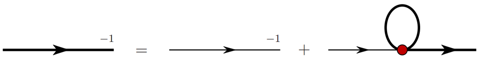
Figure 2.
Diagrams of off-shell GPDs for kaons, where .
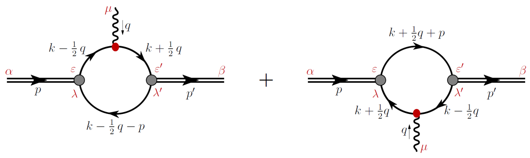
Figure 3.
Kaon off-shell vector GPD: in Eq. (21), we only plot . upper panel – The off-shell GPDs . – black dotted line; – red solid line; – blue dashed line; – purple dotdashed line. lower panel – The off-shell GPDs . – black dotted line; – red solid line; – blue dashed line; – purple dotdashed line.
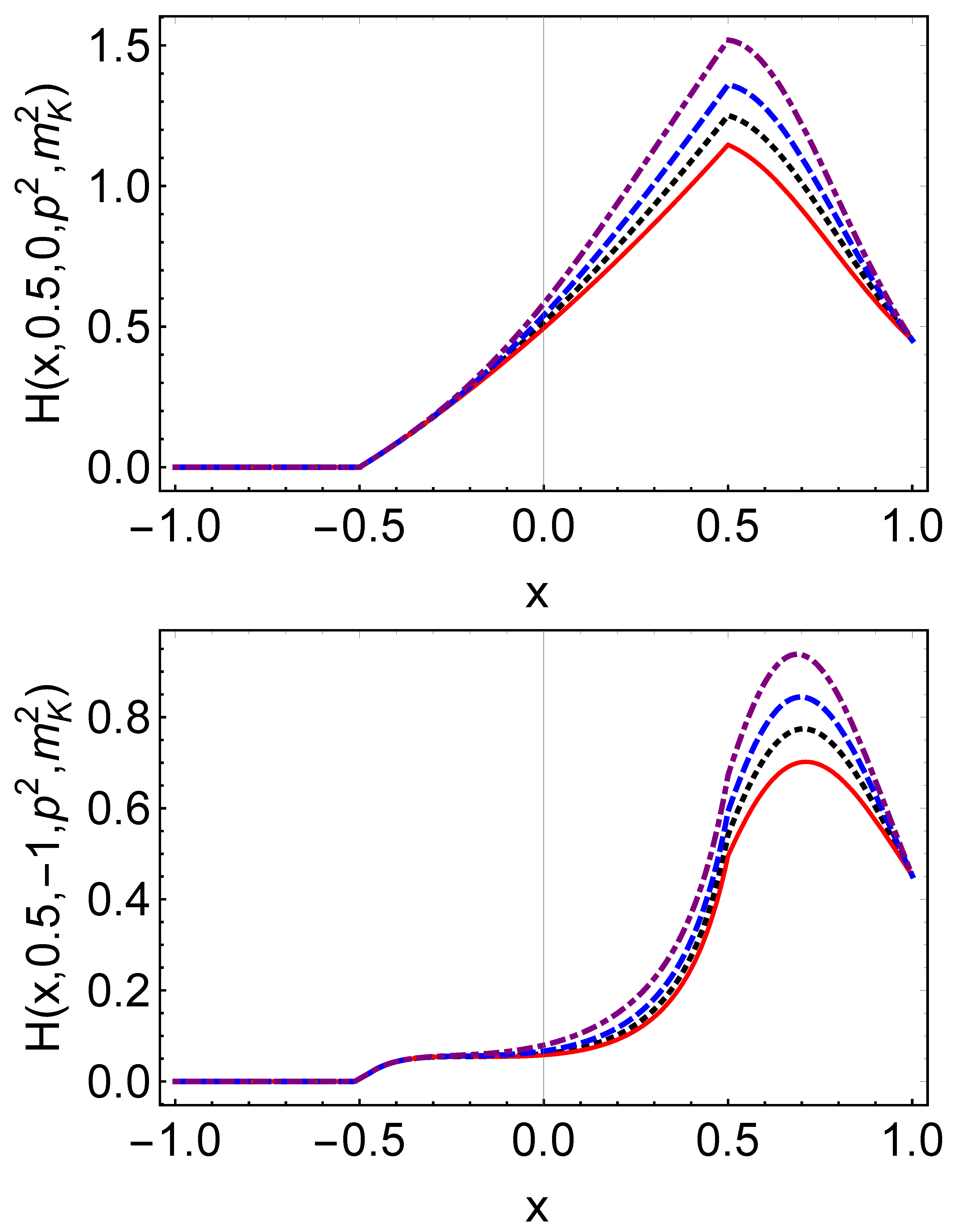
Figure 4.
Pion off-shell tensor GPD: in Eq. (22), we only plot . upper panel – The off-shell GPDs . – black dotted line; – red solid line; – blue dashed line; – purple dotdashed line. lower panel – The off-shell GPDs . – black dotted line; – red solid line; – blue dashed line; – purple dotdashed line.
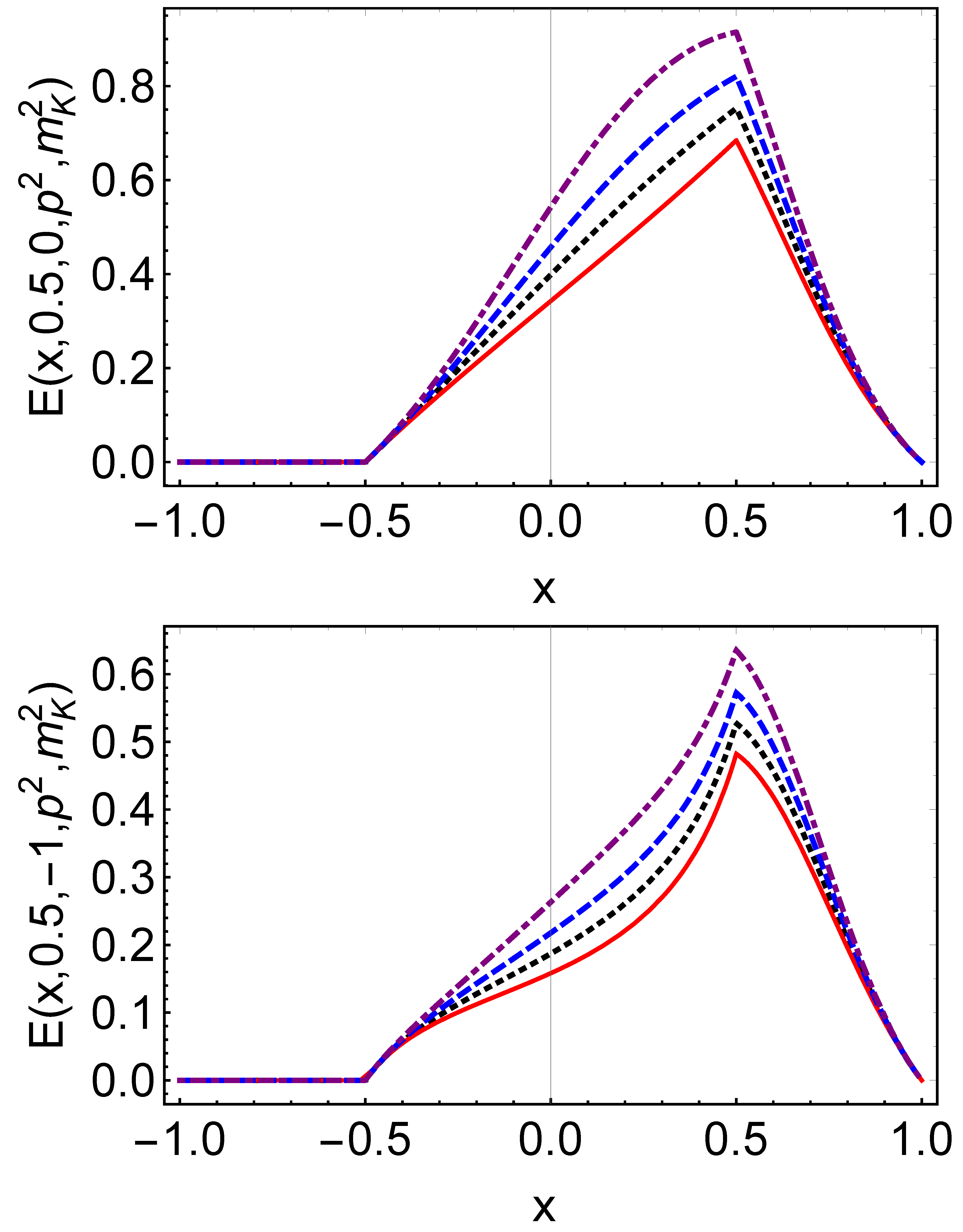
Figure 5.
The off-shell u quark PDFs of kaon: with GeV2 — orange dotted curve, GeV2 — red solid curve, GeV−2 — blue dashed curve, GeV2 — purple dot-dashed curve, GeV2 — black solid thick curve.
Figure 5.
The off-shell u quark PDFs of kaon: with GeV2 — orange dotted curve, GeV2 — red solid curve, GeV−2 — blue dashed curve, GeV2 — purple dot-dashed curve, GeV2 — black solid thick curve.
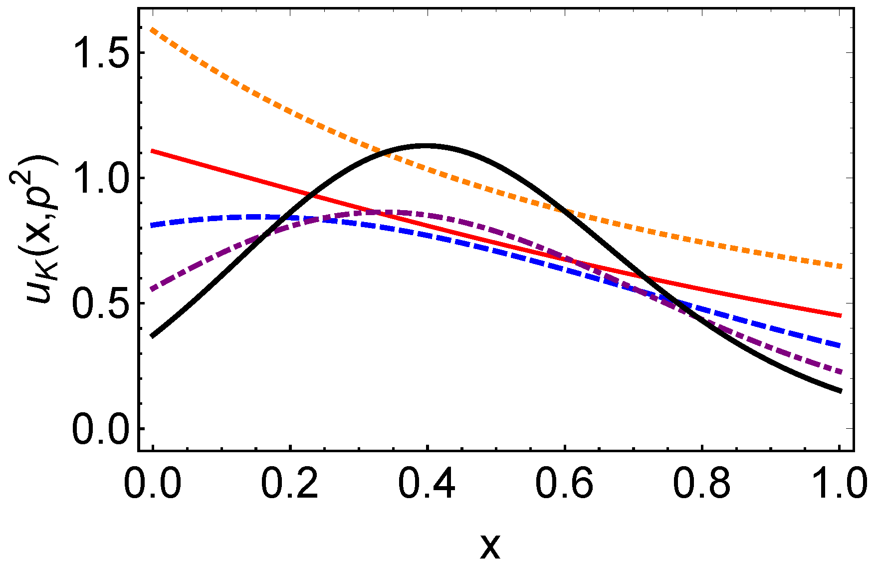
Figure 6.
Impact parameter space PDFs : upper panel – , the component first line of Eq. (41) – is suppressed in the image, and lower panel – both panels with GeV2 — orange dotted curve, GeV2 — red solid curve, GeV−2 — blue dashed curve, GeV2 — purple dot-dashed curve.
Figure 6.
Impact parameter space PDFs : upper panel – , the component first line of Eq. (41) – is suppressed in the image, and lower panel – both panels with GeV2 — orange dotted curve, GeV2 — red solid curve, GeV−2 — blue dashed curve, GeV2 — purple dot-dashed curve.
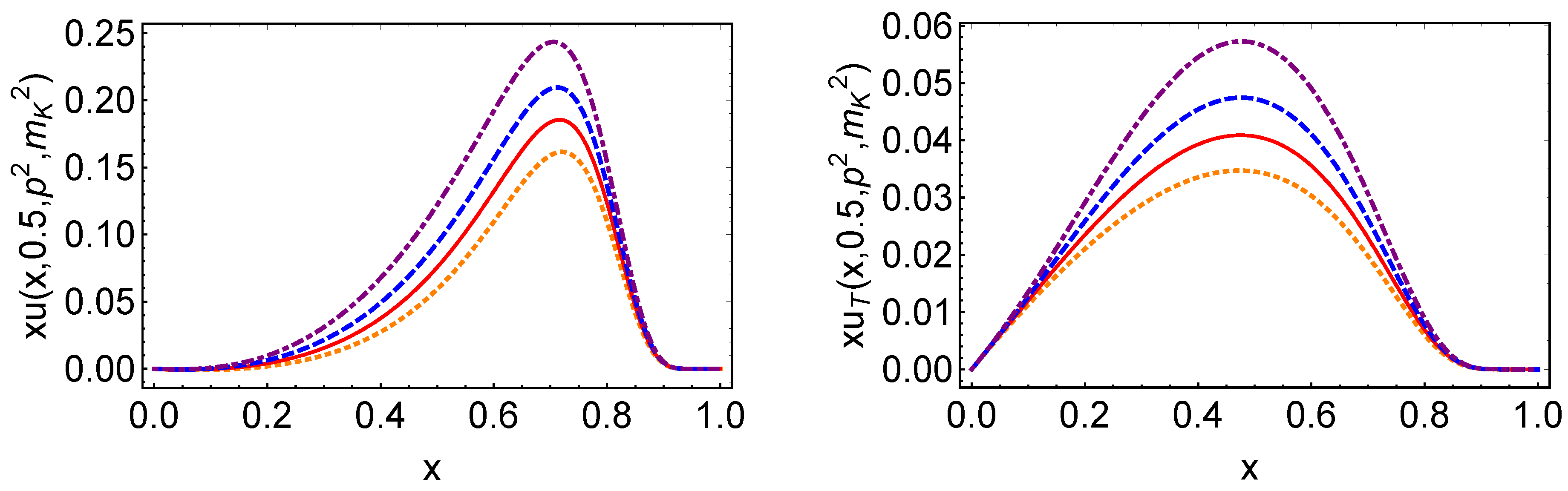
Figure 7.
Feynman diagrams illustrating the kaon TMDs within the NJL model are presented. The shaded circles denote the kaon Bethe-Salpeter vertex functions, while the solid lines represent the dressed quark propagator. The operator insertion takes the form . The left diagram corresponds to the TMDs of the up u quark, whereas the right diagram pertains to those of the strange s quark in relation to the kaon.
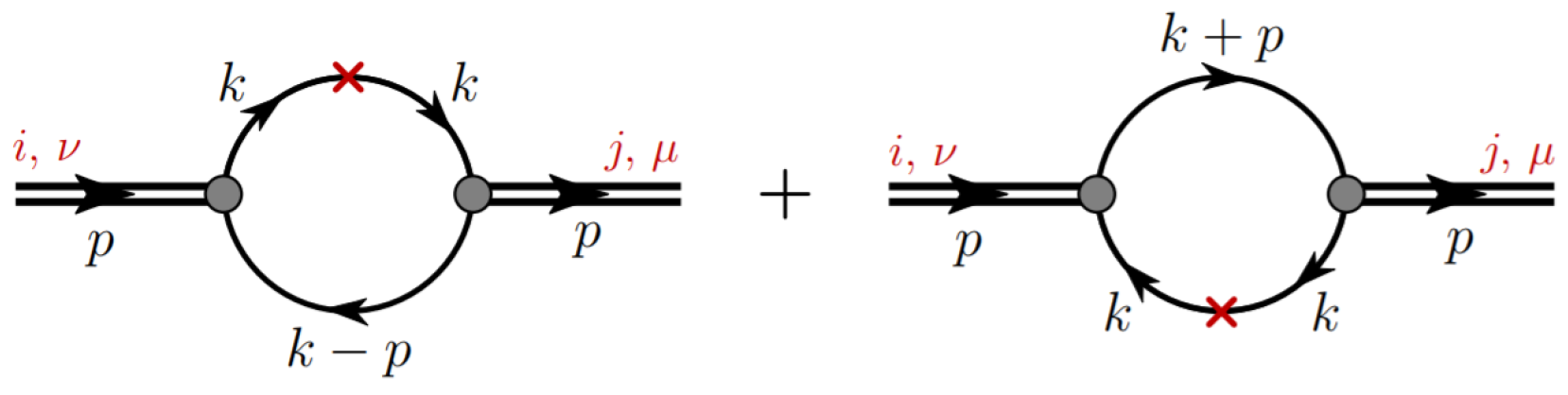
Figure 8.
Kaon TMDs: Upper Panel – The on-shell kaon TMDs represented as ; Lower Panel – The off-shell kaon TMDs denoted by
Figure 8.
Kaon TMDs: Upper Panel – The on-shell kaon TMDs represented as ; Lower Panel – The off-shell kaon TMDs denoted by
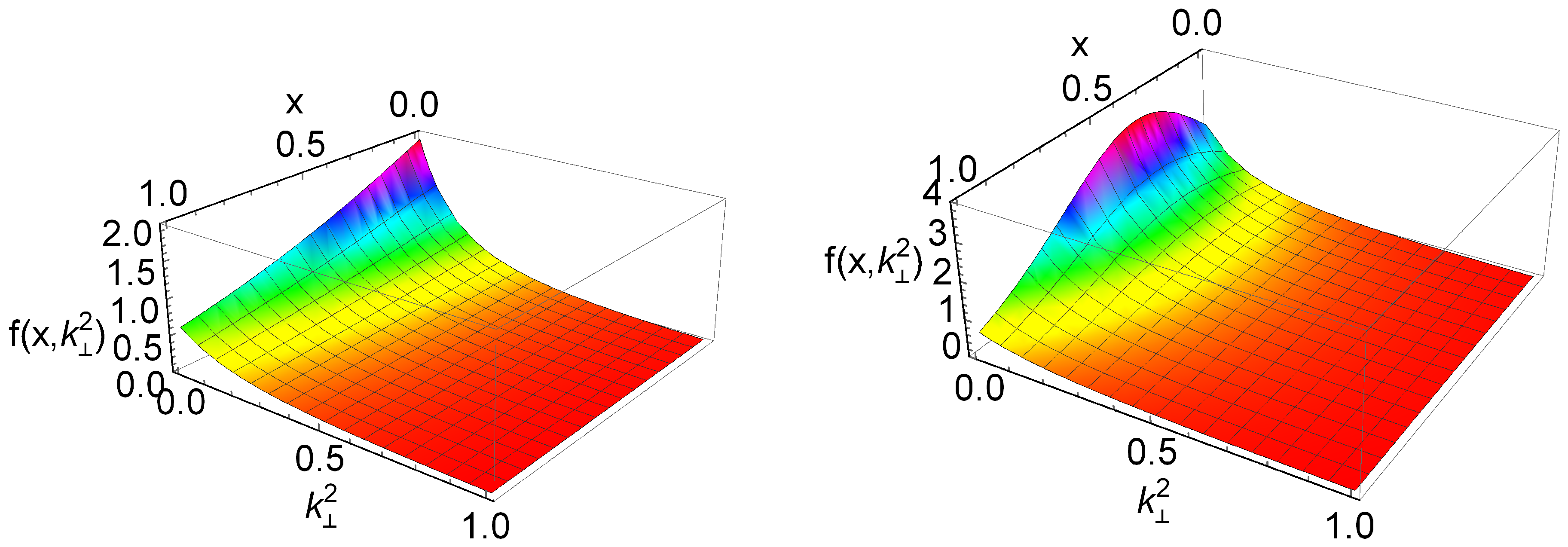

Table 1.
The parameter set utilized in our study is presented here. The dressed quark mass and regularization parameters are expressed in units of GeV, while the coupling constants are measured in units of GeV−2.
Table 1.
The parameter set utilized in our study is presented here. The dressed quark mass and regularization parameters are expressed in units of GeV, while the coupling constants are measured in units of GeV−2.
| 0.240 | 0.645 | 0.40 | 0.59 | 19.0 | 0.47 | 20.47 |
Disclaimer/Publisher’s Note: The statements, opinions and data contained in all publications are solely those of the individual author(s) and contributor(s) and not of MDPI and/or the editor(s). MDPI and/or the editor(s) disclaim responsibility for any injury to people or property resulting from any ideas, methods, instructions or products referred to in the content. |
© 2025 by the authors. Licensee MDPI, Basel, Switzerland. This article is an open access article distributed under the terms and conditions of the Creative Commons Attribution (CC BY) license (http://creativecommons.org/licenses/by/4.0/).
Copyright: This open access article is published under a Creative Commons CC BY 4.0 license, which permit the free download, distribution, and reuse, provided that the author and preprint are cited in any reuse.


