
Submitted:
01 September 2025
Posted:
02 September 2025
You are already at the latest version
Abstract
Airfoils are the key component of aircraft that are used to generate lift force to support its weight. Optimization of airfoils can significantly enhance their aerodynamic efficiency. The present study introduces a novel method of airfoil optimization that integrates Genet-ic Algorithms (GA) with Deep Learning (DL). The dataset was generated using XFOIL by varying angle of attack and Reynold’s number for various airfoil geometries. The geometry of airfoils was represented by Bezier Curve parametrization in the dataset. The generated dataset was used to train a Dual Branch Fully Connected Hybrid Activated Deep Network (DBFC-HA DN) model. The novel approach involves the integration of the trained model with the Genetic Algorithm (GA) to find the optimized solution (geometry) of the airfoil bounded within a pre-defined angle of attack range that is based on a reference airfoil. CFD analyses have been performed to verify the results of the proposed model. For NACA 65(2)-415, a 24.45% increase in lift-to-drag ratio was identified using CFD analysis at 0º angle of attack. The results were also validated using wind tunnel testing. The approach presented in the study saves computational cost and time for the optimisation of airfoils as compared to CFD and provides a basis for its use in the optimisation of airfoil performance for the relevant aerospace engineering applications.
Keywords:
Aerodynamic Shape Optimization (ASO)
; Deep Learning
; Genetic Algorithms
; Computational Fluid Dynamics (CFD)
; Aerodynamic Efficiency
1. Introduction
Optimization of airfoil shape is an important step for aircraft design required to ensure a stable, safe and economical flight. Optimization of airfoil shape is important for curtailing the fuel cost by increasing lift and reducing the drag, thus, enhancing the aerodynamic efficiency of the aircraft [1]. The optimization of airfoils is employed in designing vehicle components such as spoilers and wings, especially for high-performance aircrafts and racing cars, to enhance aerodynamics, stability, and downforce. Many techniques exist for the optimization of airfoils to increase their performance.
Particle Swarm Optimization (PSO) and Genetic Algorithm (GA) have been employed for this job with mixed results, and their utility depended on the specific optimization problem. Jiang et al. have used an improved PSO for the optimization of low Reynolds number airfoils to obtain a 12% increase in the performance [2]. Ümütlü and Kiral used genetic algorithm to optimize airfoils parametrized by Bezier Curve [3]. They performed XFOIL and CFD simulations to demonstrate that the optimized airfoils had an increased aerodynamic efficiency. Chen and Li proposed a hybrid PSO and GA technique to optimize the lift, drag, and surface pressure of an airfoil. The experimental results showed the effectiveness of the hybrid technique [4]. Similarly, Mathioudakis et al. optimized an airfoil with successful integration into a Blended-Wing Unmanned Aerial Aircraft (UAV) using GA [5]. This research work paved the way for data-based optimization of airfoils. In 2021, Li and Zhang introduced a high-fidelity Aerodynamic Shape Optimization (ASO) using a CFD-GA interface [6]. The results showed this fast optimization method for the airfoils resulted in a relative mean error of less than 0.4% as compared to CFD-based optimization methods.
The use of Machine Learning (ML) for ASO has increased because of the extensive airfoil data available nowadays. Li et al. have discussed cutting-edge algorithms for fast optimization of airfoils in their review article including GAN (Generative Adversarial Networks), CNN (Convolution Neural Networks), and ANN (Artificial Neural Networks) [7]. The article by Le Clainche et al. examines the latest advances in machine learning (ML) that are having an impact on the multidisciplinary fields of aerospace engineering, aerodynamics, acoustics, combustion, and structural health monitoring [8]. An approximate model for the prediction of aerodynamic behavior can be obtained using an extensive database (Surrogate Modelling). Recent advances in Surrogate Modelling using ML have paved the way for several techniques and algorithms utilizing the power of such low-fidelity models [9]. Researchers have used ML-based surrogate modeling for predictions of aerodynamic coefficients, load distributions, and shape optimization [10,11].
Many researchers have used various ML-based algorithms for the design optimization of their problems. The first stage is to parametrize the airfoil curve. This parametrization introduces design space for the dataset and the optimization of the airfoil. Agarwal and Sahu have discussed a unified approach to parametrize any airfoil using Bezier Curves [12]. An airfoil can be accurately parametrized using only a six-degree Bezier Curve. Wei et al. introduced a systematic approach for parametrizing an airfoil using the Bezier Curve and then used the parametrization data for airfoil optimization by employing Non-Sorted Genetic Algorithm (NSGA-II) on results obtained from XFOIL [13]. It was observed that the optimization of E387 airfoil showed an increase in the Lift to Drag ratio. CNN has also been used for the parametrization of airfoils. Li et al. optimized an airfoil using CNN coupled with surrogate modeling [14]. The results show the effectiveness of the proposed method in the case of low Reynolds number airfoils. There have been many instances where CNN has been used to parametrize airfoils for the predictions of aerodynamic coefficients which can be further optimized using GA and PSO [15,16].
Deep learning has also been employed for the aerodynamic shape optimization of airfoils. Deep Reinforcement Learning (DRL) was used to optimize 20 airfoils to prove the generality of the method. Enhancement in lift-to-drag ratio as well as substantial stall margin was noticed for the optimized airfoil [17]. Similarly, BPNN (Back Propagation Neural Network) has also been used for the prediction of aerodynamic coefficients [18,19]. Yonekura et al. utilized DRL for optimization of Turbine airfoils [20]. They observed that the training time of the model was long, but the trained model could be used for optimization in a shorter time as compared to conventional optimization methods. Researchers have used deep learning for various other tasks as well such as dynamic stall suppression and structural strength improvements [21,22].
Determining the aerodynamic performance of airfoils using wind tunnel testing and CFD simulations can be resource intensive and time-consuming. Due to this, low-fidelity sources can be used for dataset generation for deep learning applications. XFOIL is one of the interactive programs through which aerodynamic properties of airfoils can be computed. It uses panel-based computational methods due to which computational cost becomes low [23]. Morgado et al. compared the XFOIL results for an airfoil with that from CFD [24]. They observed that XFOIL gave the best prediction results overall. XFOIL has been coupled with Machine Learning for optimization of airfoils associated with wind turbines [25]. In their review article, Sharma et al. discussed using XFOIL and RFOIL (a software based on XFOIL) for quick prediction of aerodynamic performance coefficients. These results can be coupled with PSO, GA, or ML for quick optimization [26]. In recent developments, Wen et al. coupled XFOIL with airfoils fitted with Bessel polynomials and optimized them with GABP (Genetic Algorithm Back Propagation) artificial neural network [27].
To date, there is a substantial research gap in the direct integration of deep learning and Neural Networks (NN) with genetic algorithms for airfoil shape optimization (ASO). While researchers have integrated CNN with traditional optimization algorithms, coupling GA with deep learning remains an uncharted territory [28]. This novel approach leverages the strength of deep learning and genetic algorithm to solve complex optimization problems related to the fields of aerodynamics and aircraft design. As the dataset of the ML model is generated in many ways (low-fidelity and high-fidelity methods), this optimization approach is flexible to the dataset. Multi-Objective Genetic Algorithm (MOGA) can be incorporated into this design system as well. Our proposed novel method introduces the use of DL-GA integration. The results have been validated using CFD simulations and wind tunnel testing.
The optimization methodology and results are outlined in the subsequent sections. Section 2 describes the dataset and the structure of the deep-learning model. This model is incorporated into the genetic algorithm (NSGA-II) for calculation of the optimal coefficients of lift and drag. In Section 3, details of CFD set up and mesh refinement study are presented. Subsequently, results are checked against XFOIL (XFLR5) and CFD (ANSYS Fluent) simulations and are also validated by wind tunnel testing. Section 4 offers discussion on the results. The present study sets grounds for other researchers to use different datasets and investigate aerodynamic shape optimization (ASO) in different contexts.
2. Methodology for Airfoil Optimization
The main objective of our work is to get an airfoil with enhanced aerodynamic characteristics. Figure 1 shows the flowchart representing the algorithm of the approach of training and testing the data, and Figure 2 shows the approach of ASO using DBFC-HA DN integrated with GA. GA optimize the solutions based on the principles of evolution. The process starts with creating a population of potential solutions in the form of parametric vectors. The initial conditions are normally chosen randomly so that they are as dissimilar as possible. Every candidate solution is assessed by a fitness function, such as a trained model in the present case to determine the quality of the solution. The fittest individuals are selected for reproduction using selection methods such as the roulette wheel or tournament selection [29]. Some of the parents are selected to crossover, which means that their parameters are mixed to create offspring, thus encouraging new solutions. Random mutations are then applied to preserve the genetic variation and prevent the algorithm from getting stuck in local optima. This process of evaluation, selection, crossover, and mutation is repeated for many generations to enhance the population until a termination criterion is reached.
In DBFC-HA DN coupled with GA, there are two output labels: coefficient of lift and coefficient of drag. For prediction, Linear Regression uses the values of independent variables; here, the total input features/independent variables are 28, which include the upper and lower control points of the 2D airfoil (26 Control points), Reynolds number, and Angle of attack to predict the value of aerodynamic efficiency. The main goal of this study is to optimize the aerodynamic efficiency of the airfoil, defined as:
2.1. Bezier Curve Parametrization
Parametrization of an airfoil can be performed using Bezier curves. Bezier curve parameterization for airfoils uses a set of control points to define the curve shape, providing a smooth and flexible surface contour by employing Bernstein polynomials to perform interpolation between these points. This method allows precise control over the airfoil geometry, facilitating the optimization of aerodynamic parameters and airfoil design [30].
The leading and trailing edges of the two Bezier curves, which represent the bifurcation of upper and lower airfoil surfaces, must match to ensure C0 continuity and to produce a closed loop curve. The equations of Bezier Curve Parametrization include [31]:
Hence, Control points will be:
Where B is Bernstein polynomial while k is its degree, (n+1) defines the order of parametrization, t ranges from 0 to 1, i ranges from 0 to k, and P is the control point (or vertices) of the curve. Figure 3 shows the application of 6th degree Bezier Curve parametrization to represent the airfoil shape.
2.2. Dataset
The dataset consists of data generated by XFLR5, a low fidelity analysis tool, for low Reynolds number airfoils. The data for 50 airfoils have been taken by varying Reynolds numbers from 1×10⁵ to 1×10⁶ and while keeping angles of attacks from −5º to 18º. A total of 38,239 instances are available, each described by 28 predictors (features): comprising of x and y coordinates of 13 control points (6 each on upper and lower surfaces of the airfoil and C0 at the leading edge), Reynolds number, and angle of attack. The airfoil shapes were parameterized into control points using sixth-degree Bézier curves. The two response variables (target output) are CL and CD. The model was trained using 34,416 instances and evaluated with 3,823 instances per fold through a 10-fold cross-validation approach. A detailed list of the predictors is presented in Table 1.
2.3. Development of DL Model
The experiments were conducted on a Lenovo P500 ThinkStation featuring an Intel® Xeon® E5-2650 v3 processor (10 physical cores, 20 logical threads @ 2.3 GHz), 64 GB of RAM, and an NVIDIA GeForce GTX 1080 Ti GPU with 11 GB of VRAM. GPU-accelerated computations were enabled using CUDA Toolkit 11.8 and compatible NVIDIA drivers. The system ran on Microsoft Windows 10 Pro (Build 19045).
Model implementation utilized the TensorFlow CUDA framework with the Keras API for designing and training DL architectures. Key components included the Adam optimizer, EarlyStopping, and ReduceLROnPlateau callbacks for enhancing training efficiency. The evaluation was performed using scikit-learn, specifically, StandardScaler for normalization, train_test_split for partitioning, and metrics such as R2 and MSE, MAE, and RMSE for model assessment. Visualization tasks were handled with matplotlib. The input dataset included Reynolds number and angle of attack as features. These were normalized using StandardScaler to ensure zero mean and unit variance for each feature. The model outputs two key aerodynamic coefficients: the lift coefficient (CL) and the drag coefficient (CD).
This study proposes a DBFC-HA DN, a DL strategy for multi-task learning where different branches learn different outputs from the same input, for predicting CL and CD. As detailed in Table 2, the architecture begins with a shared base network that processes input features through a 128-unit Dense layer with Swish activation, selected for its smooth gradient behavior, followed by batch normalization for training stability. From this shared backbone, the network splits into two specialized branches:
CL Prediction Branch: This path begins with a 128-unit Dense layer using ReLU activation, followed by a second ReLU-activated Dense layer with 64 neurons. These layers are designed to extract and refine lift-related features. The branch concludes with a single-neuron output layer using Linear activation, ideal for continuous output.
CD Prediction Branch: Recognizing the more complex nature of drag force, this branch employs a deeper and more regularized structure. It starts with a 256-unit Dense layer using GELU activation, followed by a 128-unit GELU-activated Dense layer. A Dropout layer (rate: 10%) is included to mitigate overfitting. A final 64-unit GELU-activated Dense layer further refines the features before reaching the Linear-activated output neuron, delivering the continuous CD prediction.
2.4. Loss Function
To account for the differing importance of CL and CD in aerodynamic applications, a mean squared error (‘mse’) loss function is used. This function combines mean squared error (MSE) terms for both CL and CD but assigns asymmetric weights (0.3 for CL and 0.7 for CD) to emphasize drag predictions. This tailored weighting strategy drives the model to minimize CD errors aggressively, while preserving CL accuracy. The network is trained using the Adam optimizer, with L2 regularization (λ = 10−5) and dropout applied to prevent overfitting. The dual-branch architecture allows for task-specific feature learning, and when coupled with the loss function, the model aligns with real-world aerodynamic objectives. By amplifying CD’s contribution to the loss, the architecture achieves enhanced precision in drag prediction, crucial for optimizing wing and airfoil designs.
2.5. Activation Functions’ Hybrid
This study employs a hybrid approach to activation functions to enhance the model’s representational power. The Swish activation function [32] is used in the shared base of the network to facilitate smooth gradient flow and capture fine-grained input patterns. The Cd prediction branch utilizes GeLU activations [33], known for their probabilistic behavior, which helps in learning nuanced, context-rich features and accelerates convergence. In contrast, the Cl branch employs ReLU activations [34], which are effective for extracting sparse, discriminative features, particularly useful in learning more binary or sharply defined patterns. For the output layers of both branches, Linear activations [35] are used to preserve the continuous nature of the predicted aerodynamic coefficients. The model was further fine-tuned through hyperparameter optimization across various predictors. This strategic use of multiple activation functions allows each branch to specialize in its respective task, ultimately improving the model’s accuracy and convergence behavior.
2.6. Model Parametrization
The parameters, as illustrated in Table 3, within the DBFC-HA DN model have been tuned during training to best fit the data. The DBFC-HA DN was configured with a bifurcated architecture, employing shared layers followed by two separate output branches for CL and CD predictions. The model employs separate mean squared error (MSE) losses for lift (CL) and drag (CD) coefficient predictions. A weighted combination of these losses guides optimization, with CD assigned a higher weight (0.7) to prioritize drag prediction accuracy. CL receives a lower weight (0.3) to maintain awareness of lift dynamics. This weighting compensates for CD’s smaller physical magnitude while ensuring both aerodynamic properties influence training.
The model was compiled using the Adam optimizer, and a three-phase learning rate schedule was employed as illustrated in Table 4: Phase 1 (<50 epochs): (Initial learning rate configuration, Phase 2 (50–100 epochs): Intermediate adjustments, and Phase 3 (100–300 epochs): Final fine-tuning phase). Training was carried out for 150 epochs with a mini batch size of 64. An early stopping mechanism was implemented with a patience of 20 epochs based on validation CD R² score to prevent overfitting. The best model weights, as determined by this criterion, were saved to the file best_model.keras. To improve generalization, L2 regularization was applied with a weight decay coefficient of λ = 10-5. Furthermore, a 10-fold cross-validation strategy was adopted to ensure reliability of the model performance across the dataset.
Feature inputs were standardized using StandardScaler, while CL and CD outputs were scaled independently using separate StandardScalers to account for differing distributions. The shared backbone of the DBFC-HA DN architecture consisted of a 256-unit Swish-activated layer followed by batch normalization, then a 192-unit Swish layer with another batch normalization. The CL prediction branch followed a sequence of 128 and 64 neurons activated with ReLU, concluding with a single linear output. In parallel, the CD prediction branch used a deeper path: 256, 128, and 64 neurons with GELU activation, incorporating a dropout layer (rate = 0.1) after the second hidden layer, and ending with a single linear output node.
2.7. Sensitivity Analysis of Loss and Learning Rate with Epochs
The model was trained for 150 epochs, and the resulting learning curves are presented in Figure 4 which illustrates the overall training process. In Figure 4(a), the abscissa denotes the number of training epochs, while the ordinate indicates the loss values. The blue and green curves represent the training loss of CL and CD, respectively, and the orange and red curves represent the validation loss of CL and CD, respectively. Both curves exhibit a consistent downward trend over time indicating that the model is effectively learning from the training data while maintaining good generalization performance on unseen test data. Figure 4(b) depicts the evolution of the learning rate throughout training in terms of its performance measurement, where the abscissa again shows the number of epochs and the ordinate represents the R2 score. The plot shows that the learning rate is initially set to a high value to enable rapid learning in the early stages, but it decreases sharply to allow the model to fine-tune CL and CD. This learning rate schedule helps prevent the model from converging prematurely to a suboptimal solution and promotes better overall performance.
2.8. Ablation Study for Model Generalization
To investigate the generalization capability of the proposed DBFC-HA DN model, an ablation study was carried out using varying phase schedules in terms of epochs across three progressive training phases as illustrated in Figure 5: Phase 1 (iterations 1–50), Phase 2 (51–100), and Phase 3 (101–150). This approach was designed to analyze how different learning rate phase combinations affect the model’s ability to predict CL and CD accurately. The performance of the DBFC-HA DN model was evaluated using four widely accepted statistical metrics: R-squared (R2), root mean squared error (RMSE), mean squared error (MSE), and mean absolute error (MAE) [36]. These metrics provide a comprehensive understanding of both the accuracy (through R2) and the error magnitude (via RMSE, MSE, and MAE) of the model’s predictions. Table 4illustrates the results of this epoch variation-related study, showing the model’s performance for both CL and CD under different phase schedule settings. Among the tested combinations, the configuration using phase values of 0.0005 (Phase 1), 0.0001 (Phase 2), and 0.00005 (Phase 3) outperformed others, achieving the highest R2 scores of 0.9897 ± 0.0006 for CL and 0.9506 ± 0.0053 for CD. This indicates that the model was able to explain approximately 99% and 95% of the variance in CL and CD, respectively, suggesting a high degree of model reliability. Additionally, this configuration also resulted in the lowest RMSE and MAE values, which indicate smaller average prediction errors, further confirming its effectiveness.
The standard deviation values, obtained from ten-fold cross-validation, are relatively low, highlighting the consistency of the DBFC-HA DN performance across different data partitions. It is also worth noting that the largest predicted values for CL and CD across all configurations were 1.9556 and 0.23535, respectively, serving as a reference for the model’s prediction range. Overall, the ablation study demonstrates that careful tuning of phase schedules significantly enhances the DBFC-HA DN model’s generalization ability.
2.9. Genetic Algortihm
GA was used for airfoil optimization because of its efficiency in the solution of problems of high nonlinearity and multidimensionality. In aerodynamic optimization, there are always multiple objectives that are in conflict with each other, for instance, maximum lift and minimum drag. Many conventional approaches are unable to search for the solution space effectively when dealing with a large number of variables and non-convexity [13]. In such cases, GAs, which are based on the principles of natural selection, are capable of providing selection, crossover, and mutation for both exploration and exploitation, and they can find the global optima. The trained DBFC-HA DN model was incorporated as the fitness function to estimate the CL and CD rapidly. This approach is computationally much less intensive than performing high-fidelity simulations on all the candidate solutions. Table 5 shows the settings used for NSGA-II (Non-Sorted GA), which is used with integration of the DL model.
Where, eta is Distribution Index and Sampling Method is the Method to Initialize Population. Design space was provided from reference airfoil (Lower and Upper Bounds), Polynomial Mutation was used as the Mutation Operator, and DBFC-HA DN was used to access CL and CD values at different points in the design space.
3. Computational Fluid Dynamic Analysis
The optimization of the airfoil has been performed as using the process presented in the previous section. To verify the optimization of the airfoil, we have performed the flow simulations using Computational Flow Dynamics (CFD). Furthermore, wind tunnel tests have also been performed to validate the CFD simulations. CFD utilizes numerical methods and digital computers to solve partial differential equations (Governing flow equations). These fundamental equations, such as the Navier-Stokes equations, are discretized into a set of algebraic equations and solved using computer programs [24]. Governing flow equations (along with Spalart-Allmaras Turbulence Model) are as follows:
Equation for Spalart-Allamaras turbulence model is given below:
3.1. Mesh Generation, Refinement Study and CFD Analysis
Structured meshing of the airfoil was performed using C-Fluid Domain as shown in Figure 6. The radius of C-Fluid domain was taken as 10c, and the height of the domain was kept equal to 20c, where c is the chord length of the airfoil. The length of the domain was kept sufficiently long so that the effects of the wake behind the airfoil could be captured properly. A bias factor towards the airfoil was used for all edges of the domain to refine the mesh density near the airfoil surface and to progressively increase it away from the airfoil. For the structured mesh used, y+ value of less than 5 was ensured to enable precise near-wall turbulence modelling in case of SA model. A mesh refinement study was also performed to obtain mesh-independent solution. Figure 7 presents the results of the refinement study, and it can be observed that mesh independence was achieved at about 3.9×10⁵ (i.e. at black-filled marker) grid elements.
A two-dimensional steady state anaylysis of the problem was carried out using Ansys Fluent. Velocity inlet (Reynold’s Number = 300,000) and pressure outlet (1 atm) boundary conditions were applied to the domain. Coupled pressure-velocity coupling scheme was used in the solver. Spalart-Allmaras Turbulence Model was used with a standard set of coefficients. Residual convergence level for various equations was set as 10-6. The boundary conditions and mesh generation methods discussed in this section were employed for both the optimized and baseline airfoils.
3.2. Validation of CFD Results Using Wind Tunnel Testing
For validation of the CFD study, results obtained for analysis of optimized airfoil were validated using wind tunnel testing under the same conditions as utilized for the CFD investigation. A 3D printed physical model of the optimized airfoil was prepared and experimental tests were performed in a subsonic wind tunnel. The material used for 3D printing was PLA (Polycystic Acid). Chord length of the airfoil was 200 mm and width used was 100 mm. A view of the airfoil model mounted in the test section of the airfoil is shown inFigure 8. During the experimentation, Reynold’s Number was maintained at 300,000 and the angle of attack was varied from 0º to 15º. The lift and drag forces acting on the airfoil section were measured using a three-component balance and lift and drag coefficients were calculated using the plan form area of the airfoil section, air velocity and density. The comparison of CFD and wind tunnel results are shown in Table 6, Figure 9 and Figure 10. Table 6 presents the comparison of lift and drag coefficients obtained from CFD with experimental data. It can be observed that the maximum percentage difference in the results was 8.57 for the case of CL and 8.90 for CD. The slight differences in the results are caused by the roughness of the surfaces that arise during the manufacturing of the airfoil. In Figure 9, lift coefficient calculated by CFD analysis agrees well with the experimental data, however, drag coefficients for experimental results in Figure 10 are slightly higher which are caused by the surface roughness effects caused by 3D printing process of the airfoil section.
4. Results and Discussion
4.1. Optimization of NACA 65(2)-415 Airfoil
In this section, optimization of NACA 65(2)-415 is discussed. Profiles of optimized and original of the airfoil are shown in Figure 11. The airfoil is optimized for a Reynolds Number of 3x10⁵ and AOA ranging from -1o to 11o. As a result of optimization, the maximum camber is slightly increased, and the maximum thickness of the airfoil is decreased. Due to these optimized geometric parameters, the aerodynamic performance of the airfoil is increased as compared to the baseline airfoil. Table 7 shows the comparison of various parameters of the optimized and baseline airfoils.
According to Table 7, the optimized version has a smaller percentage thickness as compared to the baseline airfoil. The reduction in thickness results in a decrease in drag and better performance at low Reynolds number flow regime. Moreover, thinner profile results in higher CL,max, thus providing a higher peak lift to drag ratio. Location of maximum thickness of optimized airfoil is closer to leading edge as compared to that of original airfoil. It helps to create a strong suction peak early, causing the lift to increase at low angles of attack. Furthermore, it also results in smooth pressure recovery, thus reducing the flow separation at moderate angles. The optimized airfoil has a slightly higher maximum camber as compared to the baseline airfoil. Camber plays a part in the lift characteristics of the airfoil, and small increase causes greater lift generation at smaller angle of attack. Moreover, the location of the maximum camber controls the pitching moment and the lift distribution along the airfoil span. Overall, the changes in the profile of optimized airfoil are directed at reducing the camber, moving the position of the maximum camber, and increasing the camber in the region of maximum thickness.
4.2. Comparison of Airfoils Using XFOIL
As the original data was generated using XFOIL, as a first step, the parameters of the optimized airfoil have been compared with NACA 64(2)-415 using XFOIL as given in Table 8. According to XFOIL predictions, the aerodynamic efficiency is higher than the baseline airfoil in the given AOA range. The maximum aerodynamic efficiency of 86.46 is achieved at 5.5º. It can be determined from the table that at 0º, there is 26.65% increase in ηAE as compared to the original airfoil. Optimized airfoil has shown an increase in CL as well as a decrease in CD at this AOA. The optimization is evident from Figure 12, which shows plots of CL and CL/CD respectively for both airfoils. It can be seen that both of these parameters have increased over a significant range of angles of attack. Furthermore, aerodynamic efficiency is maximum for the optimized airfoil at 5.5º. Moreover, according to XFOIL results, maximum percentage increase in aerodynamic efficiency of the optimized airfoil is 93.37 at 15º which depicts the improved performance of the optimized near stalling.
Stall angle, which is also called a “critical angle of attack,” is an angle at which an airfoil undergoes a stall when it reaches it. The critical angle of attack is the maximum angle between the oncoming air and the chord line of the airfoil before the airflow over the upper surface of the wing becomes separated thus causing a stall. It is also evident from Figure 12(a) that an increase in stall angle is obtained as well for the optimized airfoil.
4.3. Comparison of Airfoils Using CFD
CFD results for verification of optimization are shown in Table 9. It can be seen that XFOIL underestimated the values of CD for both cases. XFOIL tends to underestimate CD values relative to CFD since it is based on potential flow theory with boundary layer coupling and does not solve full Navier Stokes equations to quantify the viscous effects, thus, it is less accurate in predicting flow separation and pressure drag, particularly at low Reynolds numbers. At higher AOA, near stalling, the aerodynamic efficiency of the optimized airfoil is slightly lower than the original one because optimization was aimed at increasing the ηAE over a range of 0o – 6o angles of attack rather than a specific value of AOA. However, optimization is evident at lower angles of attack where it matters the most. Figure 13 shows a comparison of aerodynamic efficiency variation for optimized and original airfoils.
4.4. Pressure Coefficeint of Optimized Airfoil
Figure 14 shows the comparison of the pressure coefficients (CP) of the optimized airfoil and the original airfoils at 0º AOA. The negative values of CP mean that pressure is below free stream pressure and vice versa. Hence, higher pressure difference across the lower and upper surfaces of the airfoil would result in greater lift generation. It can be seen from the figure that near the leading edge of the airfoil, the difference of CP for the optimized airfoil is greater than that of the original airfoil. Therefore, more lift is generated of in the case of optimized airfoil which is evident from the results of CFD in Table 9.
Figure 15 shows the distribution of CP along the normalized chord length for both the original and optimized airfoil designs at 5º AOA. As can be seen from the comparison of the CP distribution, the general trends of the two airfoils are similar, which means the aerodynamic shape of the airfoil has not been significantly changed. Again, near the leading-edge region, particularly up to normalized chord length of 0.1, both airfoils show a steep decline in CP on the lower surface, which is quite normal due to the high acceleration of air. Moreover, in this region net Cp between the upper and lower surfaces is still higher for the optimized airfoil. Between 0.2 to 0.8 chord length, the variation of CP curve for the optimized airfoil is smoother than that of the original suggesting a smooth flow in this region. Overall, the net values of CP have increased and its transitions are smooth which imply that the optimization process has improved the aerodynamic efficiency of airfoil geometry. At 5º, the average value of CP is -0.948 for upper surface and 0.325 for lower surface in case of the original airfoil. On the other hand, the average value of CP is -0.878 for upper surface and 0.302 for lower surface in case of the original airfoil.
4.5. Pressure Contours Comparison at 0º, 5 º, 10 º and 15 º AOA
For comparison between the optimized and baseline airfoils based on CFD results, pressure contours for both the airfoils have been plotted in Figure 16. By comparing the pressure contours, generation of lift by the airfoils can be understood. For the optimized airfoil at lower angles of attack (right side), it can be observed that the low-pressure area on the upper surface is more pronounced and is stretching farther along the chord towards leading as well as trailing edge. This results in improved suction effects causing an increase in lift coefficient (CL). Due to the optimization of the airfoil, higher pressure regions are more pronounced on the bottom of the airfoil resulting in an enhanced lift generation. However, at greater angle of attack of 15o, flow separation bubble behind the airfoil is more pronounced for the optimized airfoil as compared to the baseline one. This increased flow separation causes the aerodynamic efficiency of the optimized airfoil to drop below the original airfoil. However, the present study was focused on optimizing the airfoil in the range of 0o - 6o AOAs, as stated earlier, which has been accomplished successfully.
5. Conclusions
In this research work, DBFC-HA DN integrated with GA has been employed to optimize the airfoil shape with the help of the Bezier Curve parameterization. A dataset is for drag and lift coefficients of 50 airfoils is generated using XFLR5 keeping Reynolds number in the range of 1×10⁵ to 1×10⁶ and angles of attack from −5º to 18º. A deep learning model was trained using the dataset and then was incorporated as the fitness function to estimate the CL and CD using genetic algorithms. Thus, an optimized shape for the airfoil was proposed to enhance its aerodynamic efficiency for angles of attack in the range of 0o to 6o. The thickness of the optimized airfoil was reduced and the maximum camber was increased causing the drag to reduce, and aerodynamic efficiency of the optimized airfoil to increase. To verify the enhancement of optimized airfoil efficiency, computational fluid dynamics analysis of the airfoil was performed. Moreover, CFD results have been validated with the wind tunnel testing. The computational results show upto 24% increase in aerodynamic efficiency of the optimized airfoil. The use of integration of DL and GAs to optimize the airfoil geometry proves suitable for enhancement of aerodynamic properties of airfoils. The proposed methodology can be employed to optimize different airfoils under various Reynolds number and angle of attack ranges for wide variety of aerospace engineering applications.
Abbreviations
The following abbreviations are used in this manuscript:
| B | Bezier Curve Parameter |
| Bi,n | Bezier Curve; Bernstein basis polynomials |
| cb1,cω1,cb2 | SA Model Constants |
| Cd | Coefficient of Drag |
| Cl | Coefficient of Lift |
| DBFC-HA DN | Dual Branch Fully Connected Hybrid Activated Deep Network |
| DL | Deep Learning |
| fw | Blending Function |
| P | Pressure (Pa) |
| Pi | Bezier curve control point |
| t | Bezier Curve; Interval, a float between 0 and 1 |
| V | Velocity Field (m/s) |
| ηAE | Aerodynamic Efficiency |
| ν | Kinematic Viscosity/m²s-1 |
| ρ | Density/kg.m-3 |
| σ,σ1 | SA Model Constants |
| ω ̇ | Specific rate of turbulent production (1/s²) |
References
- Gui, X.; Xue, H.; Su, S.; Hu, Z.; Xu, Y. Study on aerodynamic performance of mine air duct horizontal axis wind turbine based on breeze power generation. Energy Sci. Eng. 2022, 10. [Google Scholar] [CrossRef]
- Jiang, T.; Jiang, L. Optimization of UAV Airfoil Based on Improved Particle Swarm Optimization Algorithm. Int. J. Aerosp. Eng. 2022, 2022, 1–12. [Google Scholar] [CrossRef]
- Ümütlü, H.C.A.; Kiral, Z. Airfoil shape optimization using Bézier curve and genetic algorithm. Aviation 2022, 26, 32–40. [Google Scholar] [CrossRef]
- Chen, J.; Li, H. Airfoil Optimization of Land-Yacht Robot Based on Hybrid PSO and GA. Int. J. Pattern Recognit. Artif. Intell. 2019, 33, 1959041. [Google Scholar] [CrossRef]
- Mathioudakis, N.; Panagiotou, P.; Kaparos, P.; Yakinthos, K. A Genetic Algorithm based Method for the Airfoil Optimization of a Tactical Blended-Wing-Body UAV. In Proceedings of the 2020 International Conference on Unmanned Aircraft Systems (ICUAS), Athens, Greece; 2020; pp. 1582–1589. [Google Scholar] [CrossRef]
- Li, J.; Zhang, M. Data-based approach for wing shape design optimization. Aerosp. Sci. Technol. 2021, 112, 106639. [Google Scholar] [CrossRef]
- Li, J.; Du, X.; Martins, J.R.R.A. Machine learning in aerodynamic shape optimization. Prog. Aerosp. Sci. 2022, 134, 100849. [Google Scholar] [CrossRef]
- Le Clainche, S.; Ferrer, E.; Gibson, S.; Cross, E.; Parente, A.; Vinuesa, R. Improving aircraft performance using machine learning: A review. Aerosp. Sci. Technol. 2023, 138, 108354. [Google Scholar] [CrossRef]
- Forrester, I.J.; Keane, A.J. Recent advances in surrogate-based optimization. Prog. Aerosp. Sci. 2009, 45, 50–79. [Google Scholar] [CrossRef]
- Du, X.; He, P.; Martins, J.R.R.A. Rapid airfoil design optimization via neural networks-based parameterization and surrogate modeling. Aerosp. Sci. Technol. 2021, 113, 106701. [Google Scholar] [CrossRef]
- Peters, N.; Wissink, A.; Ekaterinaris, J. Machine learning-based surrogate modeling approaches for fixed-wing store separation. Aerosp. Sci. Technol. 2023, 133, 108150. [Google Scholar] [CrossRef]
- Agarwal, D.; Sahu, P. A Unified Approach for Airfoil Parameterization Using Bezier Curves. Comput.-Aided Des. Appl. 2022, 19, 1130–1142. [CrossRef]
- Wei, X.; Wang, X.; Chen, S. Research on parameterization and optimization procedure of low-Reynolds-number airfoils based on genetic algorithm and Bezier curve. Adv. Eng. Softw. 2020, 149, 102864. [Google Scholar] [CrossRef]
- Li, J.; et al. Low-Reynolds-number airfoil design optimization using deep-learning-based tailored airfoil modes. Aerosp. Sci. Technol. 2022, 121, 107309. [Google Scholar] [CrossRef]
- Zhang, Y.; Sung, W.J.; Mavris, D.N. Application of Convolutional Neural Network to Predict Airfoil Lift Coefficient. In Proceedings of the 2018 AIAA/ASCE/AHS/ASC Structures, Structural Dynamics, and Materials Conference; 2018. [Google Scholar] [CrossRef]
- Du, Q.; Xie, Y.; Yang, L.; Li, L.; Zhang, D.; Xie, Y. Airfoil design and surrogate modeling for performance prediction based on deep learning method. Phys. Fluids 2022, 34, 015111. [Google Scholar] [CrossRef]
- Liu, J.; Chen, R.; Lou, J.; Wu, H.; You, Y.; Chen, Z. Airfoils Optimization Based on Deep Reinforcement Learning to Improve the Aerodynamic Performance of Rotors. Aerosp. Sci. Technol. 2023, 143, 108737. [Google Scholar] [CrossRef]
- Ahmed, S.; et al. Aerodynamic Analyses of Airfoils Using Machine Learning as an Alternative to RANS Simulation. Appl. Sci. 2022, 12, 5194. [Google Scholar] [CrossRef]
- Ayman, T.; et al. Deep Learning-Based Prediction of Aerodynamic Performance for Airfoils in Transonic Regime. In Proceedings of the 2023 NILES Conference, Oct. 2023. [Google Scholar] [CrossRef]
- Yonekura, K.; Hattori, H.; Shikada, S.; Maruyama, K. Turbine blade optimization considering smoothness of the Mach number using deep reinforcement learning. Inf. Sci. 2023, 642, 119066. [Google Scholar] [CrossRef]
- Liu, J.; Chen, R.; Lou, J.; Hu, Y.; You, Y. Deep-learning-based aerodynamic shape optimization of rotor airfoils to suppress dynamic stall. Aerosp. Sci. Technol. 2023, 133, 108089. [Google Scholar] [CrossRef]
- Zhang, Q.; et al. Optimized design of wind turbine airfoil aerodynamic performance and structural strength based on surrogate model. Ocean Eng. 2023, 289, 116279. [Google Scholar] [CrossRef]
- Drela, M. XFOIL: An Analysis and Design System for Low Reynolds Number Airfoils. In Lecture Notes in Engineering; Springer: Berlin, Germany, 1989; pp. 1–12. [CrossRef]
- Morgado, J.; Vizinho, R.; Silvestre, M.A.R.; Páscoa, J.C. XFOIL vs CFD performance predictions for high lift low Reynolds number airfoils. Aerosp. Sci. Technol. 2016, 52, 207–214. [Google Scholar] [CrossRef]
- Song, X.; Wang, L.; Luo, X. Airfoil optimization using a machine learning-based optimization algorithm. J. Phys.: Conf. Ser. 2022, 2217, 012009. [CrossRef]
- Sharma, P.; Gupta, B.; Pandey, M.; Sharma, A.K.; Nareliya Mishra, R. Recent advancements in optimization methods for wind turbine airfoil design: A review. Mater. Today: Proc. 2021. [CrossRef]
- Wen, H.; Sang, S.; Qiu, C.; Du, X.; Zhu, X.; Shi, Q. A new optimization method of wind turbine airfoil performance based on Bessel equation and GABP artificial neural network. Energy 2019, 187, 116106. [Google Scholar] [CrossRef]
- Agarwal, D.; Sahu, P. (2022). A unified approach for airfoil parameterization using Bezier curves. Comput. Aided Des. Appl. 2022, 19, 1130–1142. [Google Scholar] [CrossRef]
- Qureshi, S.A.; Mirza, S.M.; Rajpoot, N.M.; Arif, M. Hybrid diversification operator-based evolutionary approach towards tomographic image reconstruction. IEEE Trans. Image Process. 2011, 20, 1977–1990. [Google Scholar] [CrossRef]
- Agarwal, D.; Sahu, P. A unified approach for airfoil parameterization using Bezier curves. Comput.-Aided Des. Appl. 2022, 19, 1130–1142. [CrossRef]
- Said Mad Zain, S.A.A.A.; Misro, M.Y.; Miura, K.T. Generalized Fractional Bézier Curve with Shape Parameters. Mathematics 2021, 9, 2141. [Google Scholar] [CrossRef]
- Mercioni, M.A.; Holban, S. P-swish: Activation function with learnable parameters based on swish activation function in deep learning. In Proceedings of the 2020 International Symposium on Electronics and Telecommunications (ISETC); IEEE; 2020; pp. 1–4. [Google Scholar]
- Lee, M. Mathematical analysis and performance evaluation of the gelu activation function in deep learning. J. Math. 2023, 2023, 4229924. [Google Scholar] [CrossRef]
- Bai, Y. RELU-function and derived function review. SHS Web Conf. 2022, 144, 02006. [Google Scholar] [CrossRef]
- Kiliçarslan, S.; Celik, M. Parametric RSigELU: a new trainable activation function for deep learning. Neural Comput. Appl. 2024, 36, 7595–7607. [Google Scholar] [CrossRef]
- Hsiao, W.W.-W.; Qureshi, S.A.; Aman, H.; Chang, S.-W.; Saravanan, A.; Lam, X.M. Artificial intelligence-enabled predictive system for Escherichia coli colony counting using patch-based supervised cytometry regression: A technical framework. Microchem. J. 2025, 193, 113206. [Google Scholar] [CrossRef]
Figure 1.
A flowchart depicting the training and testing phases of DBFC-HA DN, utilized as a fitness function within the GA.
Figure 1.
A flowchart depicting the training and testing phases of DBFC-HA DN, utilized as a fitness function within the GA.
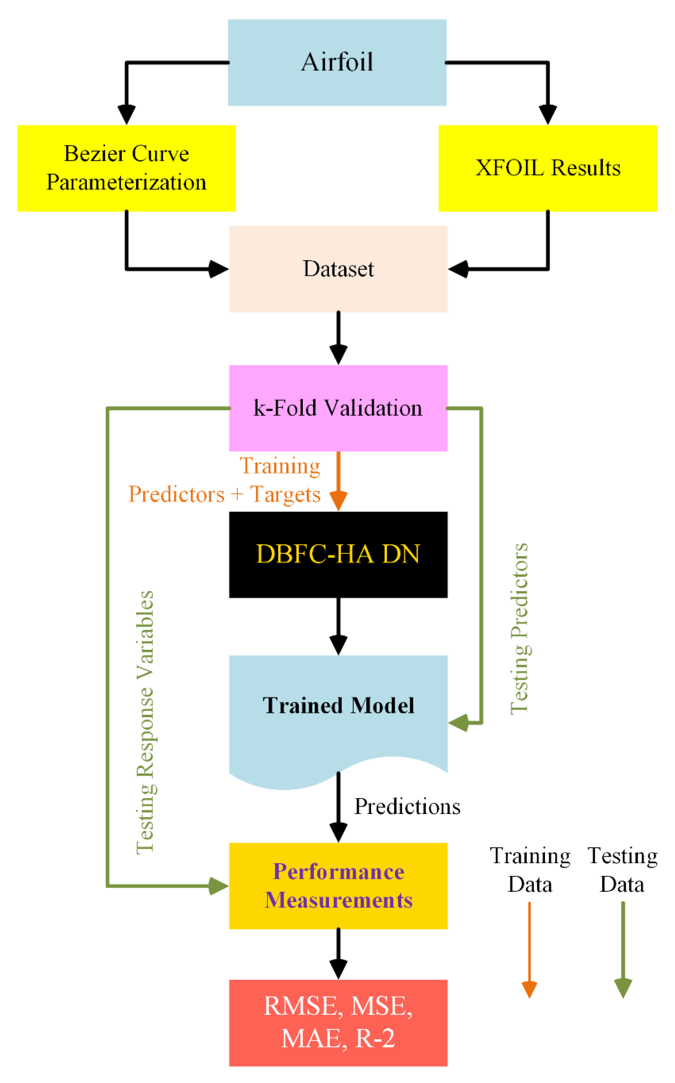
Figure 2.
A flowchart illustrating the application of ASO through the evolutionary cycle of the genetic algorithm, with DBFC-HA DN incorporated as the fitness function.
Figure 2.
A flowchart illustrating the application of ASO through the evolutionary cycle of the genetic algorithm, with DBFC-HA DN incorporated as the fitness function.

Figure 3.
Bezier curve parametrization of airfoil (y/c and x/c are normalized coordinates) [28].
Figure 3.
Bezier curve parametrization of airfoil (y/c and x/c are normalized coordinates) [28].
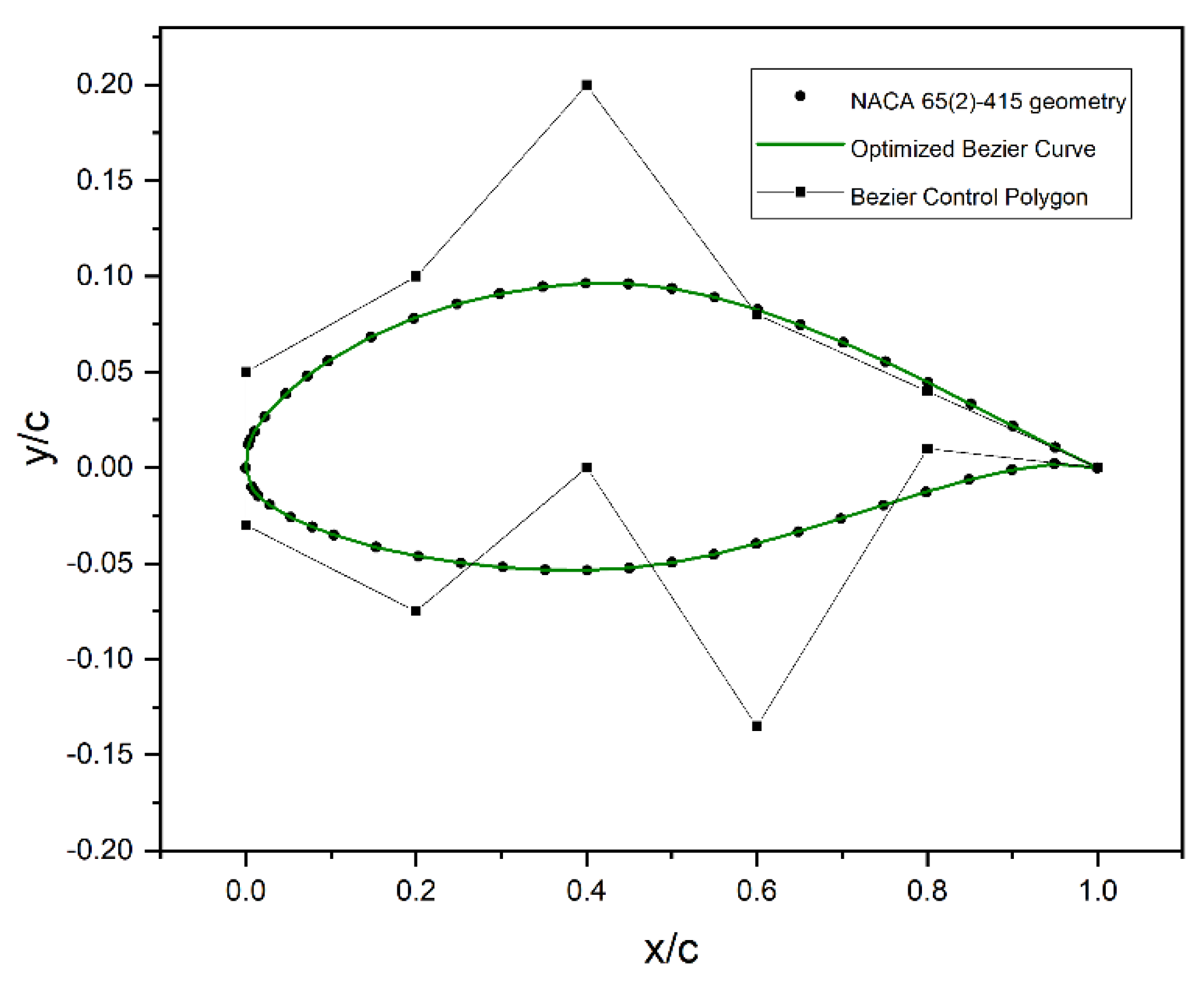
Figure 4.
Training phase exploration for the computation of CL and CD, (a) variation of loss of aerodynamic coefficients in training and validation phases, and (b) R2 variation with epochs for aerodynamics parameterization.
Figure 4.
Training phase exploration for the computation of CL and CD, (a) variation of loss of aerodynamic coefficients in training and validation phases, and (b) R2 variation with epochs for aerodynamics parameterization.
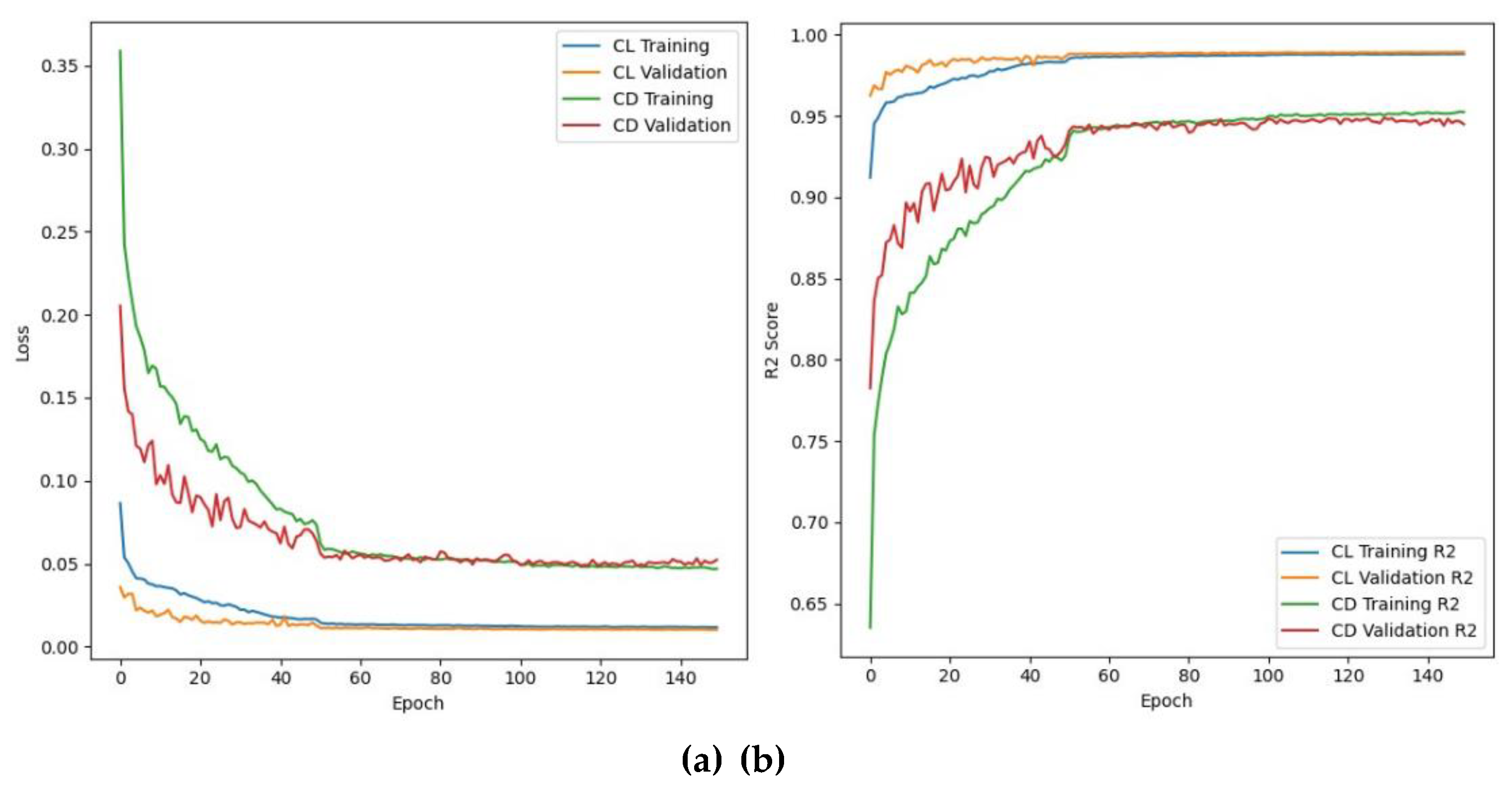
Figure 5.
Learning rate against the Epoch-variation schedule based on three phases trialed in three groups (Table 4).
Figure 5.
Learning rate against the Epoch-variation schedule based on three phases trialed in three groups (Table 4).
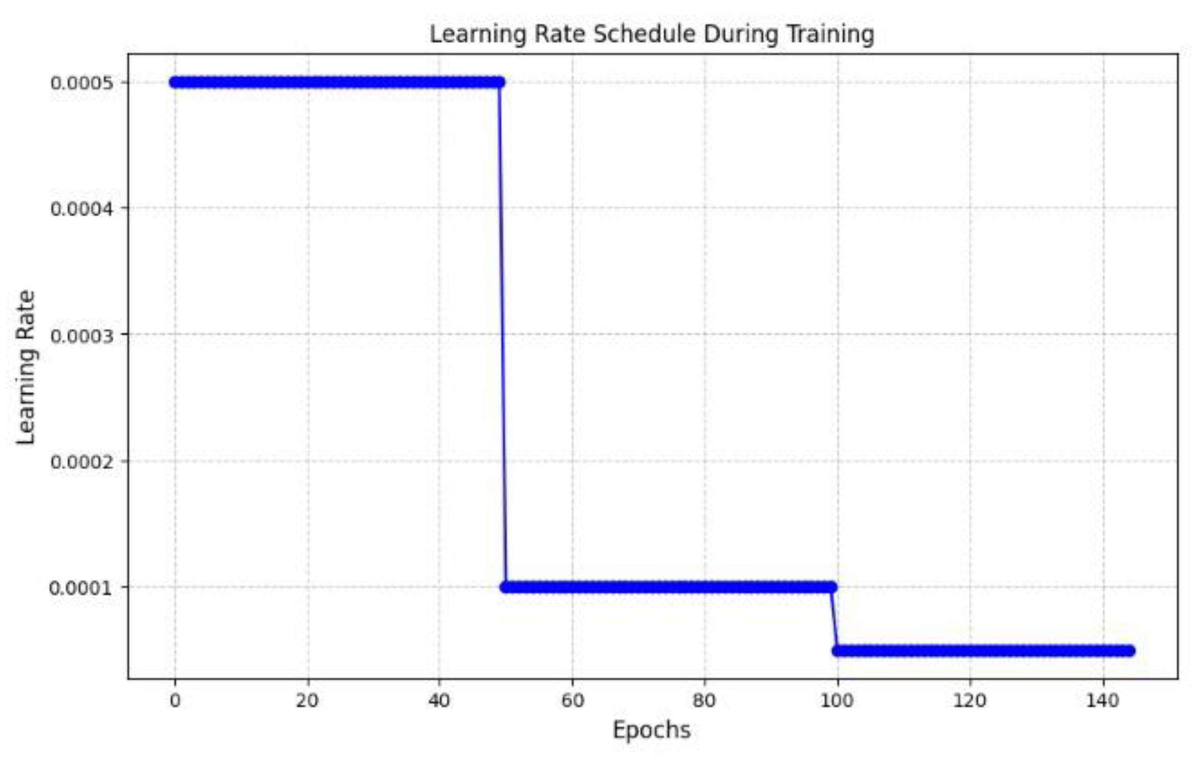
Figure 6.
C-Mesh for Airfoil CFD.
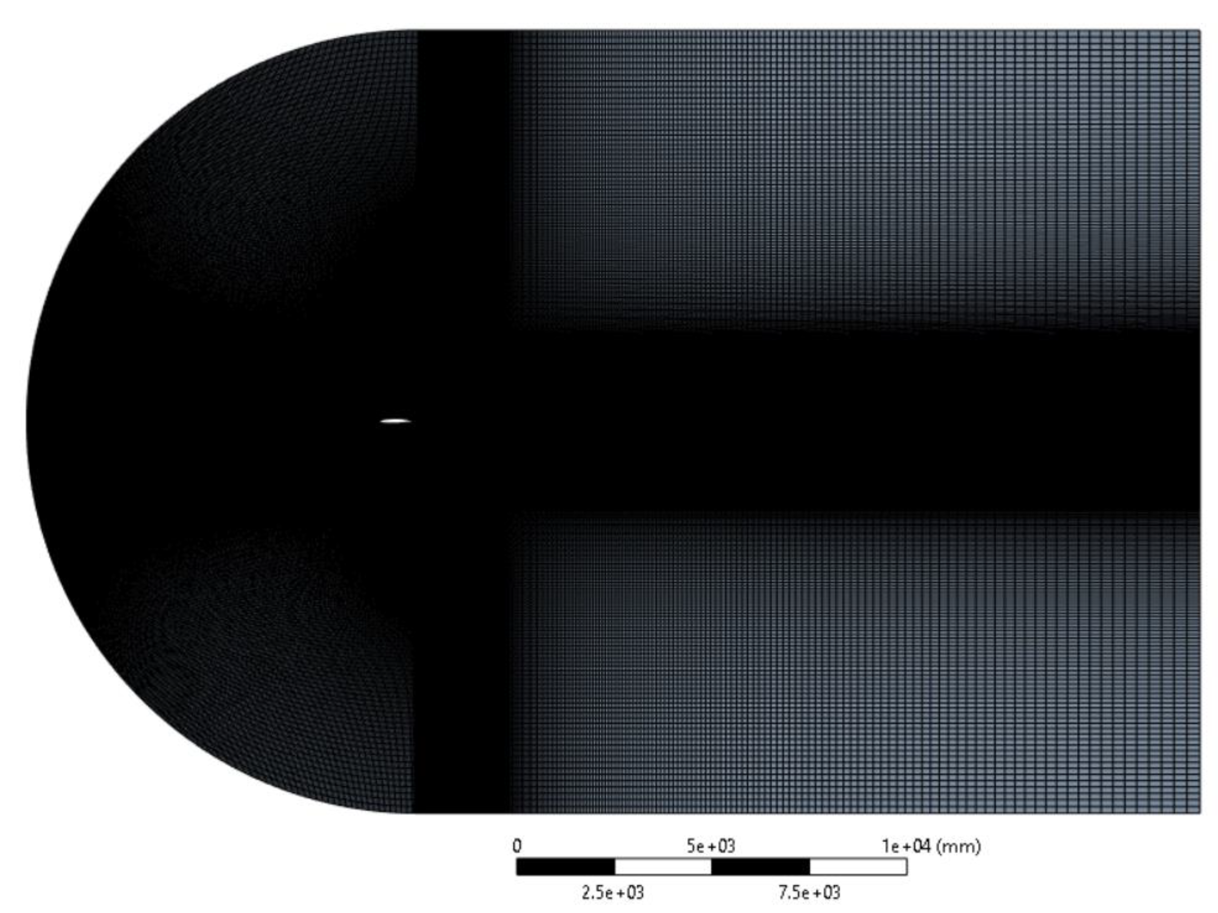
Figure 7.
Mesh refinement study.
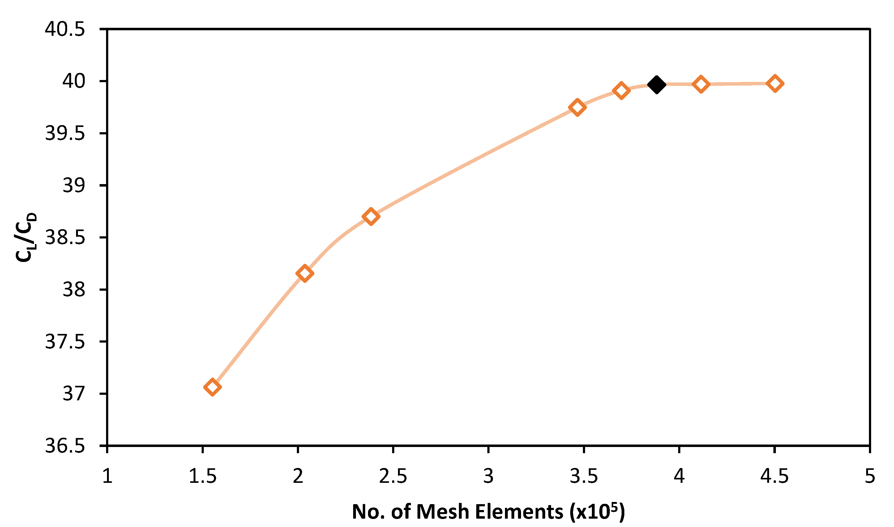
Figure 8.
Experimental setup for subsonic wind tunnel testing.
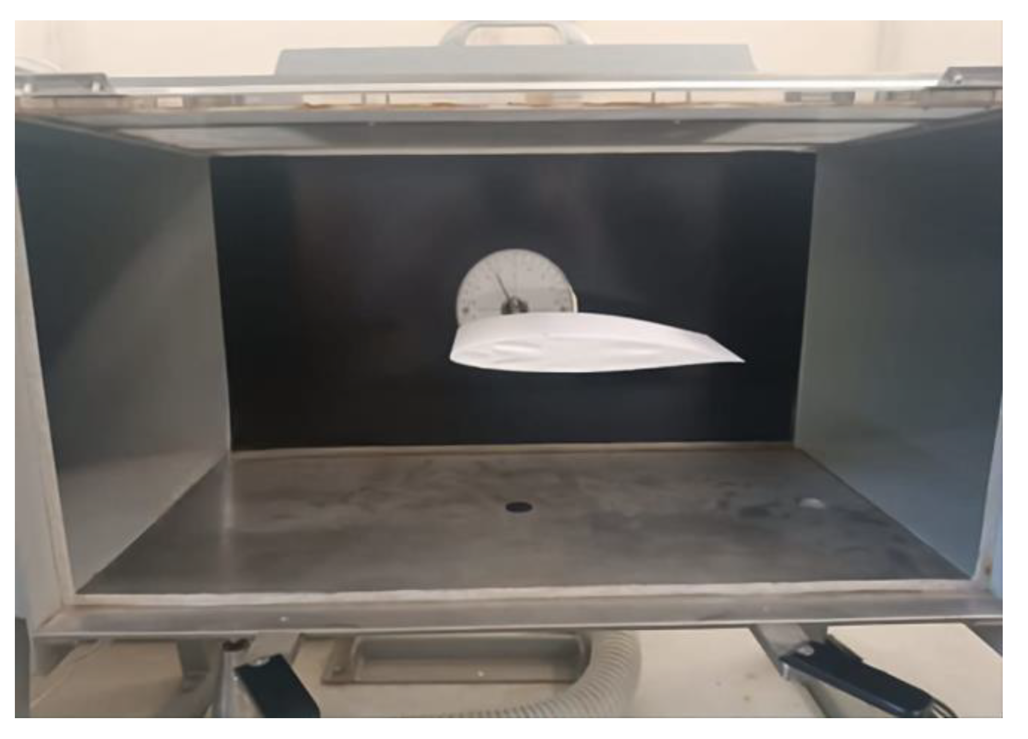
Figure 9.
Validation of the CFD results for lift coefficient of optimized airfoil.
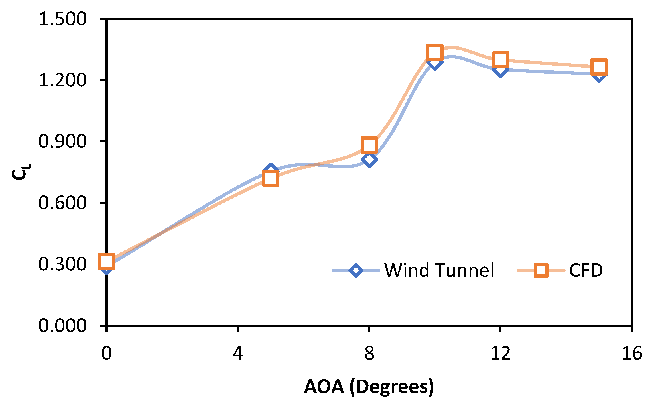
Figure 10.
Validation of the CFD results for drag coefficient of optimized airfoil.
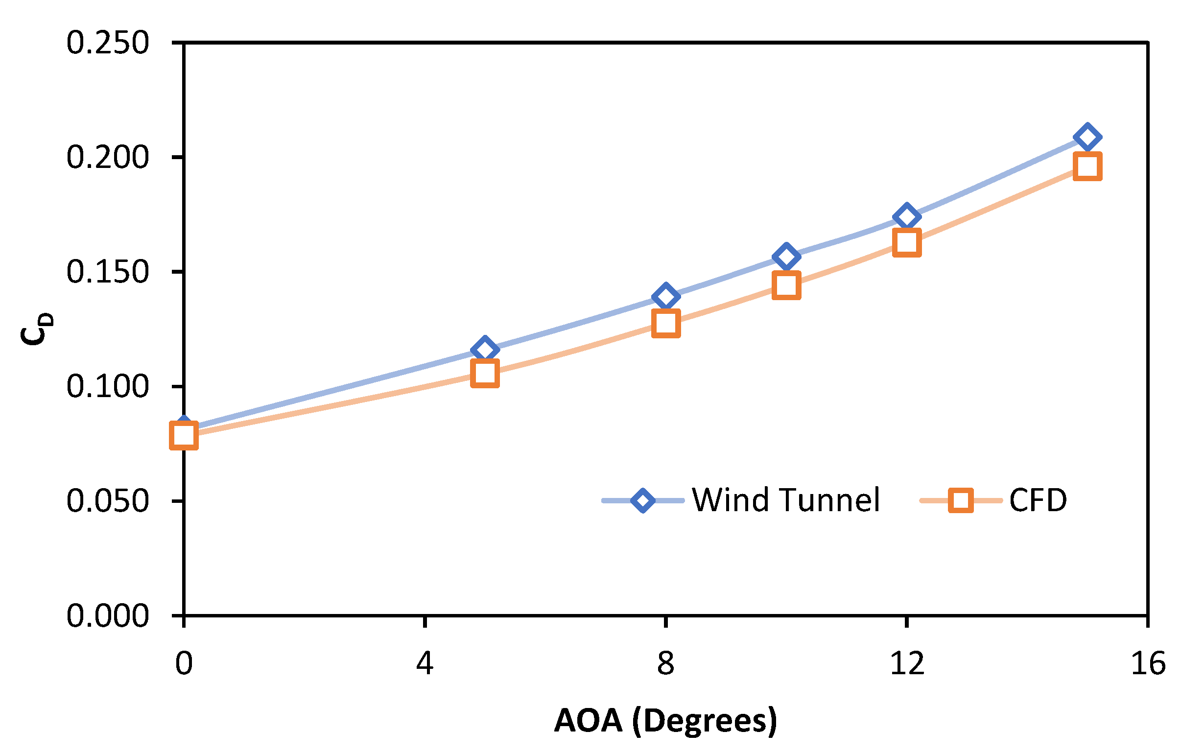
Figure 11.
Comparison of the profiles of baseline and optimized airfoils.
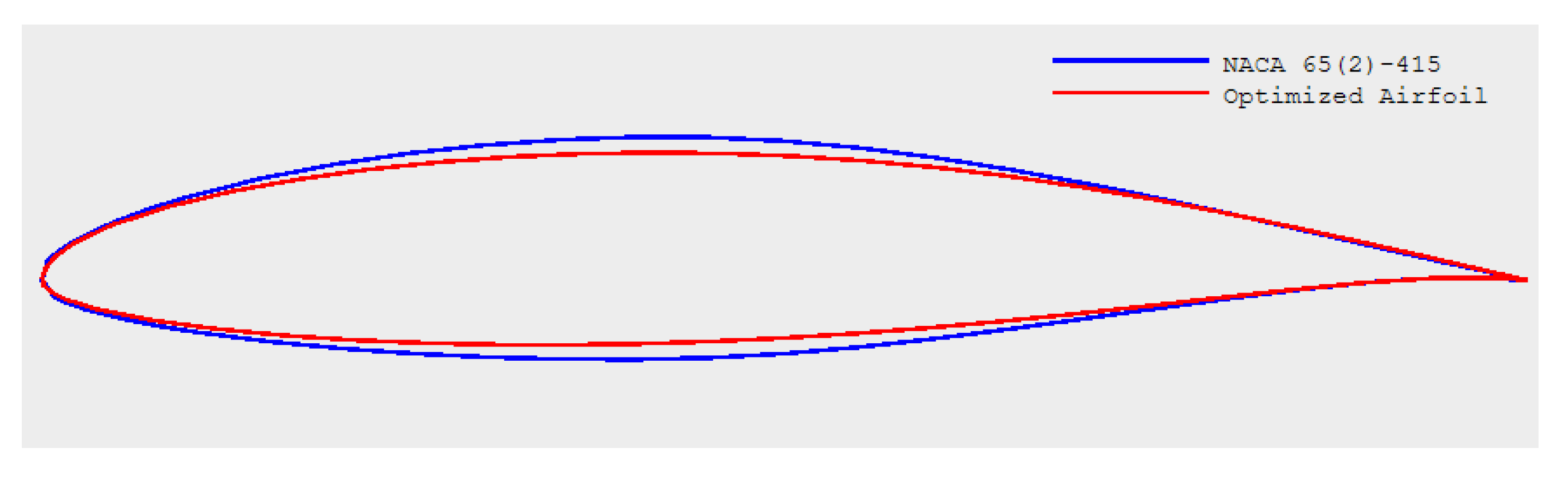
Figure 12.
Comparison of (a) CL vs. AoA (b) CL/CD vs. AOA for optimized and original airfoils.
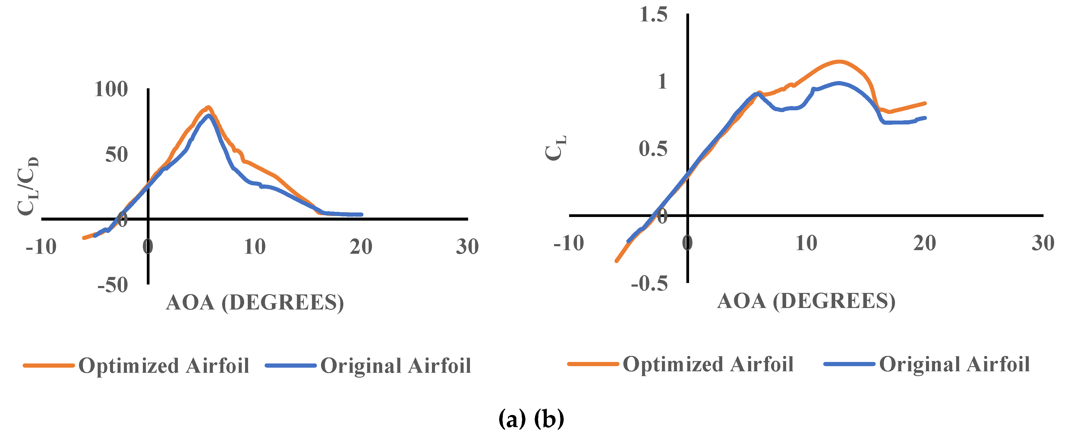
Figure 13.
Comparison of CFD results for optimized and original airfoils.
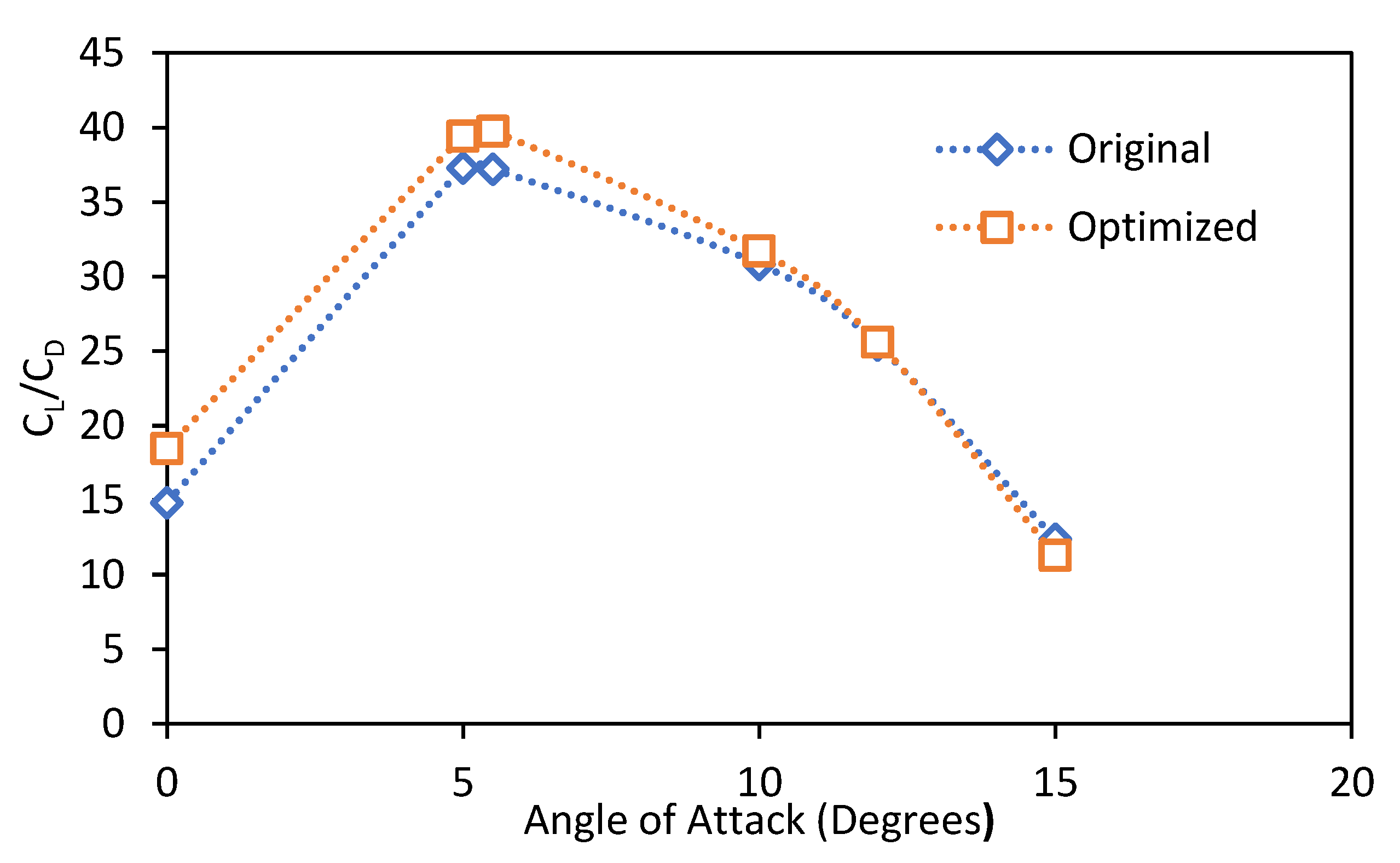
Figure 14.
CP of Original vs. Optimized Airfoil at 0º AOA.
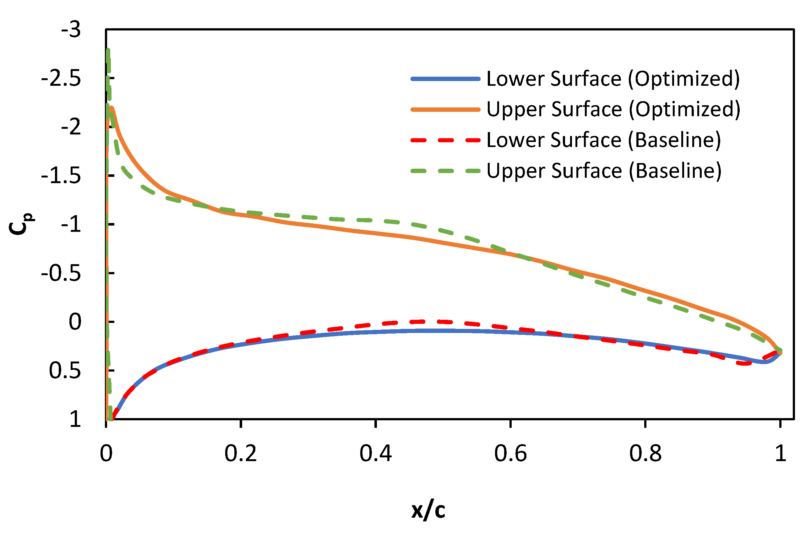
Figure 15.
CP of Original vs. Optimized Airfoil at 5º AOA.
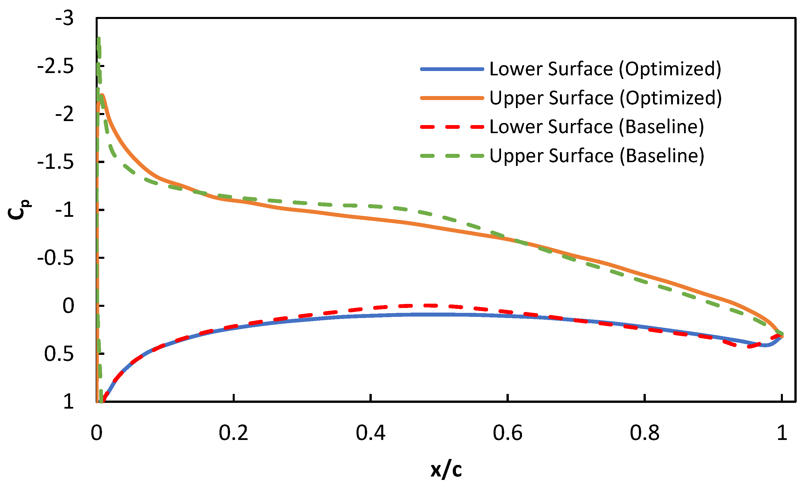
Figure 16.
Pressure contours for original (left) vs. optimized (right) airfoil at 0º(a,b), 5º(c,d), 10º(e,f), 15º(g,h) angles of attack.
Figure 16.
Pressure contours for original (left) vs. optimized (right) airfoil at 0º(a,b), 5º(c,d), 10º(e,f), 15º(g,h) angles of attack.
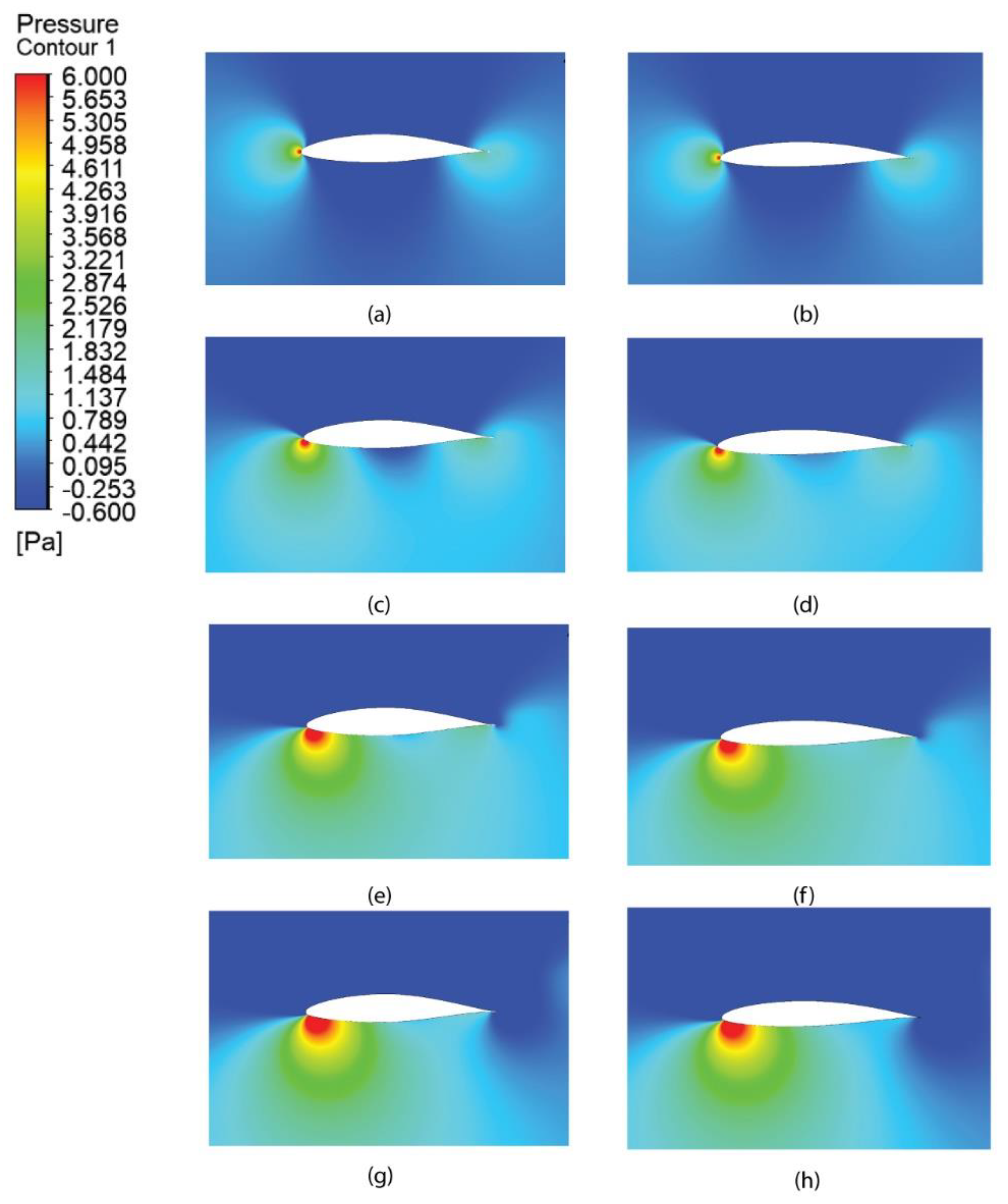

Table 1.
Details of predictors used in DBFC-HA DN with a cardinality of 28.
| Input Features | Cardinality |
|---|---|
| Lower curve control points (x coordinates) | 7 |
| Upper curve control points (x coordinates) | 6 |
| Lower curve control points (y coordinates) | 7 |
| Upper Lower control points (y coordinates) | 6 |
| Angle of attack | 1 |
| Reynold’s number | 1 |
Table 2.
A layer-wise overview of the model, detailing types, parameters, and activation functions, designed to optimize performance while maintaining computational efficiency.
Table 2.
A layer-wise overview of the model, detailing types, parameters, and activation functions, designed to optimize performance while maintaining computational efficiency.
| Layer | Neurons count | Activation function | Purpose |
|---|---|---|---|
| Input | 28 | X | Inputs are fed to the model instance-wise |
| Dense (Shared) | 256 | Swish | Feature extraction with smooth gradients |
| BatchNorm | X | X | Normalizes activations |
| Dense (Shared) | 192 | Swish | Higher-level features |
| BatchNorm | X | X | Normalizes activations |
| Branch: CL | |||
| Dense | 128 | ReLU | Lift-specific features |
| Dense | 64 | ReLU | Lift-specific features |
| Output (CL) | 1 | Linear | Unbounded* CL prediction |
| Branch: CD | |||
| Dense | 256 | GELU | Drag-specific features |
| Dense | 128 | GELU | Nonlinear drag relationships |
| Dropout | 0.1 | X | 10% Regularization |
| Dense | 64 | GELU | Final drag features |
| Output (CD) | 1 | Linear | Unbounded* CD prediction |
*The term "unbounded" is used to emphasize that the model’s predictions for aerodynamic coefficients like CL (lift) and CD (drag) are not artificially constrained to a fixed range (e.g., [0, 1] or [-1, 1]).
Table 3.
Model parameterization details for DBFC-HA DN.
| Parameter | Configuration |
|---|---|
| Model Type | Dual Branch Fully Connected Hybrid Activated Deep Network |
| Loss Function | ‘mse’ |
| Compilation Loss | CL: 0.3, CD: 0.7 |
| Optimizer | Adam |
| Learning Rate | Phase 1 (<50 epochs) Table 4 |
| Schedule | Phase 2 (50-100) Table 4 |
| Phase 3 (100-300)Table 4 | |
| Training Epochs | 150 |
| Batch Size | 64 |
| Early Stopping | Patience=20 (val_cd_r2_score) |
| Model Checkpoint | Save best weights to ‘best_model.keras’ |
| Regularization | L2 (λ=10-5) |
| K-Fold Validation | 10 partitions (folds) |
| Feature Scaling | StandardScaler |
| Target Scaling | Separate StandardScalers for CL/CD |
| Shared Layers | 256(swish), BN, 192(swish),BN |
| CL Branch | 128(relu), 64(relu), 1(linear) |
| CD Branch | 256(gelu), 128(gelu), Dropout(1/10), 64(gelu), 1(linear) |
Table 4.
Performance measures for DBFC-HA DN Model with phase schedules.
| Phase 1 (1-50) | Phase 2 (50-100) | Phase 3 (100-150) | Measure | CL | CD |
|---|---|---|---|---|---|
| 0.001 | 0.005 | 0.0001 | R2 | 0.9872 ± 0.0010 | 0.9410 ± 0.0053 |
| RMSE | 0.0809 ± 0.0030 | 0.0809 ± 0.0030 | |||
| MSE | 0.0065 ± 0.0005 | 0.0001 ± 0.0000 | |||
| MAE | 0.0546 ± 0.0029 | 0.0037 ± 0.0001 | |||
| 0.0005 | 0.0001 | 0.00005 | R2 | 0.9897 ± 0.0006 | 0.9506 ± 0.0053 |
| RMSE | 0.0725 ± 0.0018 | 0.0725 ± 0.0018 | |||
| MSE | 0.0053 ± 0.0003 | 0.0000 ± 0.0000 | |||
| MAE | 0.0436 ± 0.0015 | 0.0034 ± 0.0001 | |||
| 0.002 | 0.001 | 0.0002 | R2 | 0.9889 ± 0.0013 | 0.9470 ± 0.0061 |
| RMSE | 0.0752 ± 0.0043 | 0.0752 ± 0.0043 | |||
| MSE | 0.0057 ± 0.0007 | 0.0000 ± 0.0000 | |||
| MAE | 0.0475 ± 0.0050 | 0.0039 ± 0.0001 |
*Standard Deviation of ten-fold cross-validation is followed by ±. **Largest Cd is 0.23535 and largest Cl is 1.9556.
Table 5.
Settings of Genetic Algorithm.
| Parameter | Value/Setting |
|---|---|
| Population Size | 100 |
| Sampling Method | FloatRandomSampling() |
| Crossover Operator (crossover) | SBX(prob=0.9, eta=15) |
| Mutation Operator (mutation) | PolynomialMutation(prob.=10-4, eta=20) |
| Eliminate Duplicates | TRUE |
| Termination Criteria (termination) | No. of Generations = 500 |
| Maximize | CL |
| Minimize | CD |
| Fitness Test/ Function | DBFC-HA DN Model |
Table 6.
Validation of CFD results with wind tunnel testing.
| AOA (Degrees) | CL Wind Tunnel | CD Wind Tunnel | CL CFD | CD CFD | % Diff. CL | % Diff. CD |
|---|---|---|---|---|---|---|
| 0 | 0.290 | 0.081 | 0.313 | 0.079 | 8.00 | 3.29 |
| 5 | 0.754 | 0.116 | 0.719 | 0.106 | 4.62 | 8.90 |
| 8 | 0.812 | 0.139 | 0.881 | 0.127 | 8.57 | 8.42 |
| 10 | 1.287 | 0.157 | 1.333 | 0.144 | 3.60 | 8.00 |
| 12 | 1.252 | 0.174 | 1.299 | 0.163 | 3.70 | 6.47 |
| 15 | 1.229 | 0.209 | 1.264 | 0.196 | 2.83 | 6.11 |
Table 7.
Comparison of Geometric properties of baseline and optimized airfoils.
| Property | NACA 65(2)-415 | |
|---|---|---|
| Baseline | Optimized | |
| Percentage Thickness | 14.99 | 12.90 |
| Maximum Thickness Position (%) | 39.94 | 38.64 |
| Maximum Camber (%) | 2.20 | 2.24 |
| Maximum Camber Position (%) | 50.05 | 52.15 |
Table 8.
Comparison of lift and drag coefficients predictions for optimized and original airfoils by XFOIL.
Table 8.
Comparison of lift and drag coefficients predictions for optimized and original airfoils by XFOIL.
| AOA | CL (Original) |
CD (Original) |
CL (Optimized) |
CL (Optimized) |
ηAE (Original) | ηAE (Optimized) |
% Increase |
|---|---|---|---|---|---|---|---|
| 0 | 0.308 | 0.012 | 0.328 | 0.010 | 25.133 | 31.830 | 26.646 |
| 5 | 0.848 | 0.011 | 0.818 | 0.010 | 73.957 | 84.110 | 13.728 |
| 5.5 (Max.) | 0.888 | 0.011 | 0.881 | 0.010 | 78.459 | 86.460 | 10.197 |
| 10 | 0.849 | 0.031 | 1.083 | 0.025 | 27.359 | 43.337 | 58.403 |
| 15 | 0.887 | 0.082 | 1.266 | 0.061 | 10.803 | 20.890 | 93.371 |
Table 9.
Airfoil performance predictions for optimized and original using ANSYS Fluent (CFD).
| AOA | CL (Original) |
CD (Original) |
CL (Optimized) |
CD (Optimized) |
ηAE (Original) |
ηAE (Optimized) |
% Increase |
|---|---|---|---|---|---|---|---|
| 0.00 | 0.242 | 0.016 | 0.288 | 0.016 | 14.834 | 18.461 | 24.455 |
| 5.00 | 0.790 | 0.021 | 0.810 | 0.021 | 37.289 | 39.404 | 5.672 |
| 5.50 | 0.838 | 0.023 | 0.857 | 0.022 | 37.209 | 39.749 | 6.827 |
| 10.00 | 1.194 | 0.039 | 1.199 | 0.038 | 30.828 | 31.717 | 2.883 |
| 12.00 | 1.270 | 0.050 | 1.280 | 0.050 | 25.400 | 25.600 | 0.787 |
| 15.00 | 1.223 | 0.099 | 1.141 | 0.101 | 12.382 | 11.297 | −8.763 |
Disclaimer/Publisher’s Note: The statements, opinions and data contained in all publications are solely those of the individual author(s) and contributor(s) and not of MDPI and/or the editor(s). MDPI and/or the editor(s) disclaim responsibility for any injury to people or property resulting from any ideas, methods, instructions or products referred to in the content. |
© 2025 by the authors. Licensee MDPI, Basel, Switzerland. This article is an open access article distributed under the terms and conditions of the Creative Commons Attribution (CC BY) license (http://creativecommons.org/licenses/by/4.0/).
Copyright: This open access article is published under a Creative Commons CC BY 4.0 license, which permit the free download, distribution, and reuse, provided that the author and preprint are cited in any reuse.


