Submitted:
30 August 2025
Posted:
01 September 2025
You are already at the latest version
Abstract
This study presents an inverse approach utilizing neural networks to support the initial parameter estimation for air-dropped packages. The research is motivated by the growing need for accurate and autonomous systems in aerial delivery missions, particularly in environments where satellite navigation signals (e.g., GPS) are unavailable or degraded. In the first step, a forward neural network is trained to predict key flight parameters—range, flight time, and impact velocity—based on predefined initial conditions such as drop velocity, angle, and height. In the second step, an inverse neural network is developed to estimate these initial conditions based solely on the desired outcome parameters. A hybrid computing architecture combining simulation and neural modeling is proposed to generate sufficient training data and reduce computational cost. The results demonstrate that the proposed inverse model can accurately reconstruct the initial parameters under both deterministic and random test scenarios, provided that the input values lie within the well-represented domain of the training set. The approach offers a robust, low-cost alternative to traditional methods, potentially enabling real-time mission planning and decision support for humanitarian, scientific, or military applications.
Keywords:
air-dropped packages
; relief supplies
; neural network
; forward mode
; inverse problem
; hybrid computation
1. Introduction
The process of airdrops, regardless of their purpose (humanitarian aid, rescue materials, scientific research), is complex and requires strict coordination of multiple services, appropriate equipment, and adherence to required regulations. The success of such missions is influenced by many interdependent factors. The most important of these include:
- ▪
- Accuracy defining the drop zone, dependent on data from navigation systems (GPS, GLONASS, INS),
- ▪
- Maneuverability, mainly dependent on the aerodynamics of the capsule, but also on the structural strength (acting g-forces),
- ▪
- Achievable range, which allows for dropping the cargo from a safe distance, thereby minimizing potential losses while maintaining safety conditions,
- ▪
- Achievable object speed, which in turn minimizes the time required to deliver the airdropped cargo,
- ▪
- Flight profile, which allows for low-altitude flight,
- ▪
- Weather conditions, mainly those whose effects cannot be predicted (atmospheric turbulence, wind shear, and gusts),
- ▪
- All kinds of human factors, such as pilot or operator skills, or their availability.
Airdrops are mainly carried out using airplanes and unmanned aerial vehicles (UAV). The primary goal is to drop humanitarian aid (primarily medicines, specialized equipment, or other sensitive cargo) by quickly delivering essential resources to areas cut off from land communication routes, affected by natural disasters, armed conflict, or other crisis situations. Another specific type of mission involves the airdrop of resources such as underwater gliders, which are widely used in ocean observations [1]. In such cases, the proper water entry of the glider is crucial to prevent its destruction. For each type of these operations, methods based on airdrop dynamics modeling and control optimization are known for both cargo loading flight operations and airdrop flight operations [2,3].
Extremely important aspect concerning the cargo airdrop process is the issue of safety. Its assessment process is complex, mainly due to the strong interconnections between human, machine, and environment, but also due to the high demands placed on such missions. One example of a method used for safety assessment is the improved System-Theoretic Process Analysis-Bayesian Network (STPA-BN) method. This is a system theory-based safety analysis method. Its purpose is to understand how a lack of control over the system can lead to unsafe situations. The STPA-BN method enables real-time decision support for pilots by estimating the probability of losses in case of a single fault or failure. The authors of article [4] propose the application of a novel risk analysis method that integrates STPA and Bayesian Networks (BN) along with elements such as Noisy-OR gates, the Parent-Divorcing Technique (PDT), and sub-modeling for remote piloting operations. For quantitative safety assessment methods, Bayesian Networks themselves are used. They model cause-and-effect relationships between events and serve to calculate probabilities.
The article [5] takes the topic of airdropping heavy equipment (over 1 ton), often used in military and humanitarian missions. The authors highlight the operational complexity of such a process, characterized by strong human-machine-environment interaction. This complexity leads to difficulties in safety assessment and numerous accidents.
In the presented article, we discuss safety, but specifically in the context of errors resulting from the improper spatial position of the cargo carrier at the moment of release. It is crucial for the aircraft or UAV carrying humanitarian aid or specialized equipment (firefighting, research) to be outside the dangerous zone. Considering all this, specifying the initial conditions V0, h0, θ0 for the cargo drop is a very important issue. It frees the carrier’s operator from the need to calculate, mainly the range of such cargo, thereby eliminating the so-called "human error" in this regard. This enables real-time decision-making regarding the initial conditions for the cargo drop.
Bearing in mind the methods of cargo airdrops, they can be divided into several categories:
- -
-
Non-precision cargo airdrop systems
- ○
- They are characterized by low accuracy, meaning the cargo does not always land at the intended point,
- ○
- Most commonly used during good visibility,
- ○
- These systems require a low altitude and typically involve flying over the drop zone, which is not always possible and carries a high risk of mission failure, as well as danger to the pilot and aircraft.
- -
-
Precision cargo airdrop systems
- ○
- Work on guided airdrop systems began in the early 1960s, utilizing a modified parabolic parachute [6],
- ○
- Equipped with Autonomous Guidance Units (AGU), whose elements include: a computer for calculating flight trajectory, communication devices with antennas, a GPS receiver, temperature and pressure sensors, LIDAR radar, devices controlling steering lines, and an operating panel,
- ○
- They use appropriate devices that detect the wind profile and speed,
- ○
- They allow for airdropping cargo from altitudes of over 9,000 meters with a drop accuracy of 25 to 150 meters [7],
- ○
- They utilize advanced software (Launch Acceptability Region, LAR) that calculates the area from which a drop can be made to ensure the cargo hits the target,
- ○
- Joint Precision Airdrop System, which is designed for conducting precise airdrops from high altitudes and comes in a wide range of versions depending on cargo weight (from 90 kg to 4500 kg). Equipped with a wing-type gliding parachute, it has the ability to fly in any direction regardless of wind and to change flight direction at any moment [8].
- -
-
Guided parachutes/parafoils
- ○
- They are equipped with Autonomous Guidance Units (AGU), that allow for a change in flight trajectory, including: adjusting the course mid-flight, avoiding obstacles, and precise maneuvering to reach the designated drop point,
- ○
- They have the ability to be dropped from higher altitudes and greater distances from the drop point,
- ○
- Ram-air parachutes (wing-type) are characterized by their maneuverability and ability to fly in any direction,
- ○
- Round parachutes (modified) are less maneuverable than ram-air, but have the advantage of being cheaper to produce; they are used in systems like AGAS, where pneumatic muscle actuators are used for steering,
- ○
- The parachute’s smart guidance System Joint Precision Airdrop System (JPADS) autonomously calculates the correct drop point. To do this, it uses data from global positioning, weather models, and advanced mathematical operations, allowing it to reach the target on its own based on the received coordinates.
Determining the area where cargo should be airdropped to reach its target is crucial in precision airdrop technology and constitutes a highly complex task that requires considering many factors. The main elements influencing this process are: wind field modeling, the flight dynamics of the cargo with a parachute, algorithms for predicting the drop target, and error compensation and real-time correction. In practice, this process requires modeling the cargo’s flight trajectory from the point of release to impact, taking into account all aerodynamic forces and atmospheric conditions. This, in turn, involves advanced algorithms and measurement technologies that enable the determination of the optimal point in the air so that the cargo lands within the intended, relatively small area on the ground. In the literature [9] we can also encounter the term Calculated Aerial Release Point (CARP). Considering all these aspects (factors), it becomes reasonable to use a system that would allow for precise determination of the initial airdrop parameters before the flight and simultaneously ensure that the cargo reaches its designated target, taking into account the current flight parameters (altitude h0, velocity V0, and possibly the angle θ0 at which the drop is to occur). Such conditions are fulfilled by the proposed inverse algorithm, which enables the determination of the required initial parameters — including V0, h0, and θ0 — based on the desired landing location and target parameters. This approach effectively supports pre-flight planning and can be integrated with on-board systems to enhance precision in cargo delivery under varying flight and environmental conditions. The feasibility and efficiency of solving inverse problems using neural networks — even in complex, highly non-linear systems — has been confirmed in other fields such as robotics. For instance, in the work of [10], inverse kinematics problems in 6-DOF manipulators were successfully addressed using MLP-based networks with additional segmentation and error correction strategies, resulting in both high accuracy and low computational cost.
In order to determine the search area for a dropped cargo, mainly in conditions of limited visibility (night, fog), a multifaceted approach is used, combining precise pre-drop calculations, cargo tracking methods, and advanced post-drop search methods. The main element of this process is forecasting the drop zone. In the initial stage of this process, the probable drop zone is calculated based on precise navigation data of the aircraft (e.g., from a GNSS system) at the moment of cargo release. It is also possible to use tracking devices that can be integrated with the dropped cargo, such as: locator beacons (e.g., ELT-type devices), GPS/GNSS trackers, radio beacons, or IoT sensors. However, it is known that navigation systems are subject to various types of interference [11]. In the context of Global Navigation Satellite Systems, the main type of interference is Radio Frequency Interference (RFI), including jamming [12]. Therefore, these interferences affecting GNSS systems can cause a complete loss of signal, data distortion, or reduced positioning precision. In each of these cases, there is a huge risk of mission failure for the cargo drop. Eliminating this problem most often involves using alternative systems, such as visual odometry systems [13] or Simultaneous Localization And Mapping (SLAM) [14]. Both the visual odometry system and SLAM can operate independently of data from GNSS systems, or they can rely on them to improve their performance. Therefore, systems used to define the cargo drop zone that utilize GPS/GNSS modules [15] have their biggest disadvantage in power consumption. This can impact their functionality and operating time, and ultimately their usability. There are also places in the world that are devoid of these types of satellite signals. Therefore, it’s impossible to use systems that require data from GPS. To address this, we can use the presented method for determining three parameters: rk, tk, and Vk, to define the impact point of the dropped cargo. Most importantly, the process of airdropping resources using the presented system does not require satellite navigation data. It relies on data generated before the planned mission. This system can also serve as pilot or operator support and can be activated when GPS data is unavailable.
Algorithms and models predicting the cargo’s flight trajectory and its potential drift also play a crucial role in forecasting the drop zone. In the presented research, only the impact point was determined, but this provides key information during a mission. For this purpose, the geometric-mass data of our capsule were used to calculate its range (rk), flight time (tk), and final impact velocity (Vk) using artificial neural networks. This minimizes the risk of improper carrier positioning in space (i.e., the dropped cargo failing to reach the designated location – ocean, earth).
Another aspect discussed regarding precision cargo airdrop systems is their reliability. It should be noted that these types of airdrops require incredibly advanced systems, which can be prone to failure. The article [16] focuses on the need to estimate the reliability of airdrop systems already at the design stage, which helps avoid costly and time-consuming field tests. If such an estimation is not possible, and additionally, in the absence of information from a damaged component, the presented system can be used as support. These are typically situations where urgent cargo delivery is required, and there’s no time or opportunity to fix such failures.
Artificial neural networks (ANN) have very wide applications in the area of scientific research. With the development of computational techniques, their involvement in a broad range of applications is faster and more effective. They also constitute a valuable tool during the design of various types of systems, making them more efficient, reliable, and at the same time innovative. The following examples of artificial neural network applications refer exclusively to applications in cargo airdrop systems. A review of available literature indicates that despite the widespread use of artificial intelligence, the number of scientific papers utilizing this area for precision airdrop applications is small. In contrast, commercial development in this sphere is highly current [17].
Research utilizing intelligent cargo airdrop systems covers a wide range of issues, aiming primarily to increase precision, but also the autonomy, reliability, and safety of the conducted mission. They find application in such scientific areas as: intelligent control and guidance algorithms, trajectory modeling and prediction, reliability and safety, and multi-sensor data fusion. The authors [18] indicate the possibility of applying intelligent control technology to increase the precision of airdrop systems (PADS). This system utilizes the reinforcement learning control strategy based on the AC architecture, operating in both windless and windy environments. The article [19] presents a trajectory planning model based on a backpropagation neural network (BPNN). Meanwhile, a genetic algorithm (GA) is utilized as an optimization algorithm for landing point accuracy, providing a database verified by the Kane’s Equation (KE) model, on which the BPNN is trained, verified, and tested. The presented research results show that the BPNN model exhibits the highest landing point precision among the three investigated models. Another example of artificial intelligence utilization for unmanned aerial vehicles is an article by Chinese scholars [20], which addresses the topic of using a deep reinforcement learning method. Additionally, an Adaptive Priority Experience Replay Deep Double Q-Network (APER-DDQN) algorithm based on Deep Double Q-Network (DDQN) was applied. An algorithm based on reinforcement learning was also used to generate effective maneuvers for a UAV agent to autonomously perform an airdrop mission in an interactive environment [21]. The training set sampling method is constructed based on the Prioritized Experience Replay (PER) method. The obtained research results confirm that the algorithm proposed by the researchers was able to successfully solve the turn-around and guidance problems after successful training. The issue of precision landing of an autonomous parafoil system using deep reinforcement learning is addressed in [22]. It should be noted that, similar to this article, a case where initial conditions are randomly selected is also analyzed to test the effectiveness of the proposed system. Besides reinforcement learning, other methods from the artificial intelligence group are also applied in the field of cargo airdrop research, such as: genetic algorithm [23,24], particle swarm optimization [25,26], and Bayesian Network [16].
Neural networks (NNs) are computational models designed based on the principles observed in biological neural systems. These models have gained widespread application across numerous scientific and engineering disciplines due to their ability to process complex data structures efficiently. The extensive use of neural networks in engineering has been thoroughly reviewed in the literature, see, i.e. [27,28]. The fundamental theoretical aspects of neural networks have been comprehensively discussed in various publications, such as [29,30,31].
Among the diverse types of neural networks, one type designed for addressing regression and inverse problems has been employed in this study. This type of network is particularly well-suited for learning complex input-output relationships by mapping a given set of input data onto an output function, formally expressed as , where and denote the input and output vectors, respectively, and represents the set of network parameters that determine its behavior.
In general, we can assume that there are two approaches to solving identification problems. The forward mode is based on the definition of an error function for the differences between the results of a numerical model and the results of an experiment (numerical or measurement). The solution is obtained by minimizing this function. This type of identification can be considered more general and stable and is therefore usually used in numerical validation. A neural network can approximate the relation between input X and output Y data in a simple way:
where: X – input vector (e.g. control parameters, material parameters), Y – output vector (e.g. observed system response, simulation result), w – set of neural network parameters (weights and biases), f(⋅) – function approximated by the neural network.
Y = f(X, w),
The inverse mode analysis approach is based on the assumption that a well-defined and mathematically consistent inverse relationship exists between outputs and inputs. Once this relationship is rigorously formulated, the process of retrieving the corresponding input parameters becomes a systematic procedure that can be executed efficiently and repeatedly with high reliability. In this approach, the neural network searches for a set of input parameters X based on a expected output Y:
where: g(⋅) – is the inverse relation approximated by a NN. Examples of the use of NN in reverse analysis are often presented in the literature [32,33,34,35].
X = g(Y, w),
The research presented in this paper focuses on an imprecise cargo airdrop system, primarily due to two key constraints: low operational cost and the ability to operate without reliance on satellite navigation signals.
Two computational models were employed: a forward analysis and an inverse analysis, integrated into a computational framework (see Figure 1). In the first Stage, initial conditions of the free-fall cargo drop were assumed: initial drop velocity V0, drop angle θ0, and drop altitude h0. Based on these parameters, key outcome variables were calculated: the horizontal range of the cargo rk, flight time tk, and impact velocity Vk.
A comprehensive mathematical model of the capsule’s trajectory was used, incorporating aerodynamic forces and numerical integration of the equations of motion. This model provides a foundation for accurately determining drop parameters. In total, 125 base data sets were generated during this Stage, along with an additional 30 test sets.
The second Stage of the system involved the development of a neural network designed to perform forward prediction — that is, to compute output values rk, tk, Vk. based on arbitrary input data within a predefined range: V0, θ0, h0. In this Stage, a simple multilayer perceptron (MLP) network with backpropagation and a single hidden layer was implemented.
In the third Stage, a numerically structured dataset similar to that of the first stage was generated, but on a much larger scale — comprising 8800 sets of numerical samples. This dataset was generated using the neural network model developed in Stage two. The purpose of this step was to significantly reduce computation time. The total time required to generate the full dataset was approximately 2.3 seconds.
In the fourth Stage, a new neural network was formulated to perform the inverse task, which required a significantly large training dataset. The objective of this model was to infer the initial conditions V0, θ0 and h0 based on the desired output values rk, tk and Vk.
System validation was carried out by comparing randomly selected reference patterns — recalculated using the original numerical (hard) method — with the results generated by the proposed neural-based computational system. For further use, only the trained neural network model from Stage four would be necessary for the end user.
2. Research Assumptions and Methods
Stage 1: Flight Assumptions and Capsule’s Mathematical Model
For the presented research, we adopt an aerodynamic capsule shape that allows for:
- ▪
- Reduced air resistance – this advantage is extremely important because it minimizes friction and air turbulence around the capsule, allowing for faster and more controlled descent,
- ▪
- Improved precision and trajectory prediction – aerodynamically shaped capsules are less susceptible to the influence of crosswinds and other atmospheric disturbances. Their flight path is more stable and easier to predict, which increases the chances of a precise airdrop,
- ▪
- Increased stability during descent – allows the capsule to maintain a constant orientation in flight, reducing the risk of uncontrolled spinning, swaying, or tumbling. This is particularly important to avoid cargo damage,
- ▪
- Reduced loads on the capsule’s structure and its contents. Laminar airflow around an aerodynamic shape minimizes the dynamic forces acting on the capsule, which reduces the risk of damage to its structure and contents, especially sensitive items such as precision measuring equipment or shock-sensitive packaged medications,
- ▪
- More stable parachute opening and deployment if one is used. In the presented research, the use of a parachute was not considered. The capsule is dropped directly, e.g., from an airplane or an unmanned aerial vehicle,
- ▪
- Additionally, if an increased descent speed is desired when rapid cargo delivery is a priority.
In summary, an aerodynamic shape is crucial for ensuring the safe, precise, and effective delivery of cargo in airdrop operations. This translates into minimizing the risk of damage and increasing the chances of mission success.
It should also be emphasized that damage to specialized measuring equipment or special medications during an airdrop involves high costs. These losses include not only the value of the equipment or medications themselves, but also potential delays in mission execution, loss of important research results, or the inability to provide immediate assistance in crisis situations. Therefore, ensuring the reliability and safety of airdrops is a priority, and the aerodynamic shape of the capsule is one of the factors that contributes to this.
To determine the range parameter, a mathematical model for the capsule under consideration had to be developed. To make this possible, several assumptions needed to be made:
- ▪
- The capsule is a rigid solid, made of resistant materials that are not easily damaged,
- ▪
- The mass of the capsule does not change with time,
- ▪
- The capsule is an axisymmetric solid,
- ▪
- The Earth occupies a fixed position in space,
- ▪
- The planes of geometric, mass, and aerodynamic symmetry are the planes ,
- ▪
- There is no wind speed.
The motion of the center of mass of the capsule will be described by equations of translational and rotational motion, well-known from mechanics [36]. Newton’s law was used to derive the equations of motion for a capsule, according to which the sum of external forces acting on an object in a chosen direction is equal to the change in momentum in that direction per unit of time. Thus, the vector equation of translational motion for the capsule’s center of mass can be written in the form [37]
where: represents the sum of all external forces in the body frame, represents the velocity of the capsule, expressed in body coordinates, represents the angular velocity vector of the body frame with respect to the inertial frame, also expressed in body coordinates.
Newton’s second law for the rotational motion of the capsule is given by:
where: represents the sum of all external moments, expressed in the capsule body frame and represents the moment of inertia matrix.
Most often, cargo is placed on standard aerial pallets such as ECDS (Enhanced Container Delivery System), Type V, or 463L and secured with nets. In our research, we assume that the cargo is airdropped in a special capsule. Figure 2 shows the references system and the external forces that act on the capsule during the flight.
We assume that the capsule’s motion occurs exclusively in the vertical plane. For such a case, considering equation (3) and (4), we can finally write the differential equations for longitudinal dynamics of the capsule [38]:
where: are the resultant forces along and body axes, is the total pitching moment acting on the capsule, is the moment of inertia about the pitch axis, is capsule mass, is the components of the velocity vector of the capsule in relation to the air in the boundary system , is the component of the angular velocity vector of the capsule body and , .
Ultimately, the forces and and moment acting on the capsule appearing in equation (5) can be written in the form:
where: is the acceleration of gravity, is the air density, is the diameter of the capsule body, is the characteristic surface (cross-sectional area of the capsule), represents the velocity vector of the centre of capsule mass in relation to the air, is the coefficient of the aerodynamic axial force, is the coefficient of the aerodynamic normal force, is the coefficient of the aerodynamic damping force, is the coefficient of the aerodynamic tilting moment, is the coefficient of the damping tilting moment.
The trajectory describes the position of the capsule’s center of mass as a function of time and external forces. Besides the gravitational force, the axial aerodynamic force has a significant impact on the shape of the capsule’s flight trajectory. It acts along the longitudinal axis of the capsule, but opposite to its axis, which has a measurable impact on its range. The second component of the resultant aerodynamic force is the normal force , which is perpendicular to the axis.
The primary source of difficulty in determining the aerodynamic forces and moments of a capsule is the determination of its aerodynamic characteristics. This concept refers to the coefficients of aerodynamic forces and moments acting on a capsule moving through the Earth’s atmosphere [39]. These coefficients, due to their dimensionless nature, allow for the comparison and evaluation of the aerodynamic properties of flight objects of different sizes [40]. The coefficient of the axial force depends on the nutation angle :
where: represents zero pitch coefficient, is pitch drag coefficient, is the nutation angle. However, the normal force coefficient mainly depends on the angle of attack .
The aerodynamic characteristics of the considered capsule were determined experimentally, in a wind tunnel.
The trajectory of the capsule’s center of mass in the Earth-fixed coordinate system is obtained using appropriate transformations. Finally, for a capsule moving in the vertical plane, we get:
Numerical integration of the capsule’s flight trajectory was performed using the fourth-order Runge-Kutta algorithm. We thus obtained the capsule’s position for each moment in time.
In summary, the proposed system for determining initial parameters for the pilot or operator can be used as a supporting system for the precise cargo airdrop process. Incorrect determination of the initial airdrop conditions can result in mission failure or difficulties in its execution. Most importantly, the proposed system takes into account the dynamics of the dropped capsule, which reflects its actual behavior.
For the assumptions made, the range of the capsule can be determined in the form of:
where: are the coordinates of the end point (cargo drop), are the coordinates of the initial point.
It should be noted that the available literature lacks specific data on airdrop speeds for packages containing medicines, firefighting equipment, or measurement capsules. Therefore, a rather broad range of drop speeds for the carrier was adopted in the research, falling within the interval of m/s. Additionally, in the research, an airdrop angle for such cargo was adopted, which directly refers to the pitch angle of the object that will be transporting this cargo.
The total mass of the capsule, including its contents, was assumed not to exceed 15 kilograms. Meteorological conditions and the necessity of defining aerodynamic characteristics for each falling object type further complicate accurate delivery. From the standpoint of precision and reducing the risk of uncontrolled cargo damage upon impact, the drop altitude should be kept as low as possible. As indicated in Table 1, the height of the cargo drop is within the range . Moreover, the UAV’s velocity at the moment of release is a key factor affecting delivery accuracy. The presented studies assumed that [41].
Table 1 presents the reference dataset consisting of 125 data samples used in the research process. It includes both the adopted input parameters — initial velocity, angle, and altitude — as well as the corresponding computed output values, namely horizontal range, flight time, and impact velocity. As indicated in footnote¹, the input parameters were divided into four distinct ranges, which allowed for their structured distribution in preparation for analysis and neural network training conducted in Stage 2.
Figure 3 shows scatter plots illustrating the relationships between the three input variables of the model and their corresponding output parameters. The 3×3 grid layout enables a clear analysis of how each input variable influences the computed results. Distinct patterns are visible — for example, the horizontal range rk increases with both the initial velocity V0 and drop altitude h0, while the effect of the drop angle θ0 appears more complex. The color scheme was selected to highlight each output variable: blue for rk, magenta for tk, and green for Vk.
Stage 2: Simple Neural Network:NN1 in a Direct Approach
In this study, the same type of neural network – a backpropagation neural network – was applied in both Stage 2 and Stage 4 computations. Due to the structure of the training data, a 3 – H – 3 architecture was adopted in Stage 2, consisting of three neurons in the input layer, H neurons in the hidden layer, and three neurons in the output layer (Figure 3). In contrast, Stage 4 employed a deeper network with two hidden layers, following a 3 – H – H – 3 architecture (refer to Figure 4). The neurons in the input layer receive the input signals and transmit them to the hidden layers through synaptic weights. The hidden layer performs a nonlinear transformation of the input data, which enables the network to model complex nonlinear relationships between inputs and outputs. The output from the hidden layer is passed to the output layer, which generates the final result vector. The learning process is carried out using the backpropagation method, which minimizes the error function, typically by means of the gradient descent algorithm. During training, the derivatives of the error with respect to the weights are computed, and the weights are subsequently updated in the direction opposite to the gradient in order to reduce the prediction error. Neural networks of this type are commonly used for classification, regression, and pattern recognition tasks. A critical aspect of their design is the selection of the number of neurons in the hidden layer (H), which directly affects the network’s ability to generalize and to avoid overfitting. A network with a 3 – H – 3 architecture is an example of a multilayer perceptron (MLP). In general terms, the operation of the network can be expressed as the following formula:
where: X – input vector (e.g. control parameters, material parameters), Y – output vector (e.g. observed system response, simulation result), w, b – set of neural network parameters (weights and biases), (⋅), (⋅) – activation functions of output and hidden layer respectively.
| (12) |
At the beginning of Stage 2, the data computed in Stage 1 had to be appropriately preprocessed. Due to the activation function used in the hidden layer ((⋅), = tanh(⋅)), which operates within the range (-1, 1), the input data also needed to be scaled to this interval. Tanh is defined by the formula:
This function (13) is commonly used in neural networks due to its normalization properties and its ability to model nonlinear dependencies. For more complex problems, advanced activation functions may be applied, such as the Universal Activation Function (UAF), see e.g. [42]. The scaling factors and the adjusted data ranges are presented in the Table 2.
For the development of the resulting free-flight parameters of the air-dropped packages, a backpropagation neural network with a 3 – H – 3 architecture was implemented (Figure 4). This network is referred to as NN1 throughout the study.
The input layer consisted of a three-element vector representing the predefined flight assumptions: V0, θ0, h0. The number of neurons H in the hidden layer was determined adaptively. During the preliminary computational phase, multiple network configurations were evaluated, with H varying from 4 to 16. It was observed that for H ≥ 7, the learning and testing errors, measured using Mean Squared Error (MSE), satisfied the predefined accuracy threshold set by the authors. Consequently, this network architecture was selected for further analysis (see Figure 3). The MSE formula is expressed as follows:
where:
– pairs of data, – reference data, – computed values.
Table 3 presents the Mean Percent Error (MPE) and Mean Squared Error (MSE, see Eq. (14)) for both the training and testing phases of the adopted network, evaluated in the normalized input space scaled to the range [–1, 1]. The results indicate a high-quality fit to the training dataset, confirming the network’s ability to accurately model the underlying functional relationships.
The trained neural network (NN1) serves a crucial role in the subsequent analytical phase, where it will be efficiently utilized to generate a comprehensive dataset. This dataset will then constitute the training set for NN2, which is designed to solve the inverse problem.
Stage 3: Generating a Big Data Set Using
At this Stage, the formulated neural network NN1 was employed to solve the direct problem. To generate the dataset, the input variables V0, θ0, and h0 were once again used to compute the corresponding output set rk, tk, and Vk by means of the NN1 network. The adopted values were divided into 20 or 22 ranges.
In total, 8800 reference data sets were generated in this manner, with the entire computational process taking 0.218889 seconds. The range of the input values used, as well as the resulting output values, was consistent with those presented in Table 1. Figure 5 presents an example of the data structure for the variable rk, shown as a function of the input parameters V0 and θ0. The plot illustrates how the generated dataset is distributed with respect to the original reference data in the input space. As shown, both datasets span the same input domain; however, the network-generated data exhibits a significantly higher density in the input space. This increased granularity provides a richer representation of the feature space, enabling more effective training of the inverse model (NN2). The clear continuity and smoothness of the generated surface also confirm the stability and generalization capability of the NN1 network across the considered input range.
Stage 4: Formulation of a Neural Network in an Inverse Approach NN2
Similar to the second Stage, a backpropagation neural network was also employed in this case. In this study, a neural network with two hidden layers was utilized to enable more effective modeling of nonlinear relationships between input features and output. Although neural networks with a single hidden layer are universal approximators of continuous functions, architectures with two hidden layers can often achieve better generalization performance and require fewer neurons to reach comparable accuracy levels [43,44,45]. In particular, when analyzing drop trajectories and performing inverse estimation of initial conditions, the use of two layers allows for capturing more complex and hierarchical data patterns [46]. Herein, a neural network featuring two hidden layers was implemented (cf. Figure 6). The training dataset for this fourth Stage comprised 8800 patterns, which were generated in the third Stage. In contrast to the preceding Stage 2, this neural network was specifically designed to perform the inverse task, i.e., computing the values of parameters that were originally considered as inputs in the direct problem —V0, θ0, h0. Such a computational procedure is essential, as reversing the process of determining the initial parameters based on the object’s range rk, along with auxiliary parameters tk and Vk, would be infeasible using classical analytical approaches, commonly referred to as “hard computing” methods also knows as a classical numerical method. Accordingly, the neural network functions as an approximative model that enables the reconstruction of input values based on the observed output parameters. This approach allows for the effective solution of the inverse identification problem under conditions of high nonlinearity and potentially ambiguous relationships between variables.
A functional representation of the NN2 network is given by:
NN2 : X(rk, tk, Vk) → 3 – H1 – H2 – 3 → Y(V0, θ0, h0)
At this Stage, the developed neural network employed a 3 – H1 – H2 – 3 architecture. The training process was completed after 457 iterations (epochs), with the number of neurons set to H1 = 6 in the first hidden layer and H2 = 6 in the second hidden layer. For the NN2 network, the Mean Squared Error (MSE), Mean Percent Error (MPE), and Maximum Percent Error (maxPE) were calculated to evaluate training performance. The results are summarized in Table 4.
Based on the data presented in the table, the highest mean percentage error was observed for the release angle θ0, amounting to 2.68%, while the lowest error was recorded for the release height h₀ at 0.88%. The maximum percentage error also occurred for the release angle, reaching 75.01%. The low mean squared error (MSE) values, on the order of 10⁻⁵ for all output variables, indicate high accuracy in reproducing the training data and a proper fit of the model to the training set.
These results confirm that the proposed neural network architecture NN2: 3 – 6 – 6 – 3 effectively models the relationship between the projection parameters and the corresponding initial values. To further illustrate the performance of the NN2 network, Figure 7 presents bar plots of the percentage error distributions for each output variable. Analysis of these plots suggests that the largest prediction errors are limited to only a few individual patterns, whereas for the majority of the data, the relative error remains low and within an acceptable range.
3. Results
The primary objective of the analysis was to determine whether it is possible to reliably estimate the corresponding initial conditions (initial velocity, release angle, and drop height) based on the known and expected range of a dropped object. Two test scenarios were conducted, differing in their approach to defining the input data for the neural network NN2.
- Case 1 – deterministic verification: in this scenario, all input variables of the network (range, flight time, and final velocity) are taken from the reference dataset (Stage 1), and the outputs generated by NN2 (V0.NN, θ0.NN, h0.NN) are compared to the corresponding values from the reference set to assess their accuracy. The errors are calculated by comparing the original data (Stage 1) with the outputs of the neural network NN2.
- Case 2 – verification using random data sets: the input data for the network are sampled from predefined intervals based on a discrete uniform distribution. The results obtained from NN2 are verified by analyzing the final parameters after conducting simulations using the estimated initial conditions.
In all cases, the results are compared in the physical (unscaled) domain, which allows for a direct assessment of their practical applicability. It is assumed that, under real-world conditions, the range value is determined based on data acquired from a GPS system.
3.1. Case 1
In this test, six data sets were selected from the training set generated in Stage 1 for verification using the NN2: 3 – 6 – 6 – 3 network, which performs the inverse task. It should be noted that these data sets overlap with those used for training the NN1 network. As shown in Table 5, this approach allows for achieving relatively low errors. In the selected set, the highest relative percentage error (EP) was 14.47% and occurred in only one case, concerning the release angle.
The results presented in Table 5 were grouped according to three analyzed parameters: initial speed, drop angle, and drop height. To further illustrate the neural network’s performance, a separate plot was generated for each of these groups, comparing the reference values with the network’s predicted values. For the initial speed plot (Figure 8), the discrepancies observed between the actual data and the neural network predictions are minimal, not exceeding a few units. This demonstrates the model’s high accuracy in estimating the initial parameters: V0.NN, θ0.NN, h0.NN.
For the drop angle plot (Figure 9), only minor discrepancies are observed. Despite the greater variability of this parameter in the data set, the predicted values remain close to the reference data, indicating good generalization capability of the model.
The drop height plot (Figure 10), on the other hand, shows that even for larger magnitudes (on the order of thousands of meters), the absolute errors remain relatively small. This indicates that the network can effectively reproduce the data across the entire range of drop heights.
In summary, the differences between the reference data and the predictions are minor in the context of the overall scale of the respective parameters, which confirms the high quality of the predictions generated by the applied neural network NN2.
3.2. Case 2
In the Type II test scenario (Case 2), 18 input data sets were generated for the inverse neural network (NN2). Each set included three key final parameters describing the course of an airdrop operation: the delivery range rk.rand, the fall time tk.rand, and the final velocity at touchdown Vk.rand. These data were generated randomly based on a discrete uniform distribution, meaning that each integer within a given interval had an equal probability of being selected. The applied intervals were as follows:
- rk.rand ∈ ⟨492, 7347⟩ [m],
- tk.rand ∈ ⟨5, 53⟩ [s],
- Vk.rand ∈ ⟨145, 292⟩ [m/s].
The use of a uniform distribution ensures the absence of any preference toward specific regions of the input space, which is particularly important in analyses aimed at evaluating the model’s response across the full spectrum of possible operational scenarios—without implicit assumptions regarding their likelihood [47,48].
Inverse problems—where the final parameters are known and the initial conditions are sought—are generally more challenging to solve than problems based on direct cause-effect relationships. In the classical forward approach (e.g., V0, θ0, h0 → rk, tk, Vk), a single set of input values typically leads to a unique solution. In the inverse direction (i.e., rk, tk, Vk → V0, θ0, h0 ), ambiguities may arise, as different initial conditions can produce similar final outcomes. Moreover, for certain combinations of final values, a physically feasible solution may not exist at all (e.g., an unrealistically short time relative to the range, or a negative drop height).
The data used in the training process (for both NN1 and NN2) do not uniformly cover the entire space of possible final parameters. This implies the existence of substantial regions within the input space for which the neural network was not previously exposed to reference data. Random sampling may inadvertently target such "gaps," increasing the risk of extrapolation beyond known regions, which can lead to inaccurate or unreliable results.
For each test sample, the minimum absolute difference (distance) between the randomly generated value and the closest value in the training dataset was calculated—separately for each parameter: rk, tk and Vk. This enabled an estimation of how "close" the test data were to the known (training) data.
The computational scheme illustrating the data flow in the analyzed scenario was as follows:
The initial parameters predicted by the inverse neural network — V0.NN, θ0.NN, h0.NN — did not have assigned reference values. As a result, it was not possible to directly compare them with the real reference values. Their quality was assessed indirectly—by analyzing the resulting final values rk.new, tk.new, Vk.new obtained from a simulation based on the initial parameters returned by NN2.
Table 6 presents the data used in the Type II test scenario, in which the inverse neural network (NN2) receives randomly assigned values of the range variable (rk.rand) and is tasked with determining the initial conditions that lead to similar outcomes. The table compares these target values (rk.rand) with the corresponding values (rk.new) obtained through simulation, following the complete inverse prediction chain. Additionally, the table includes the percentage error, absolute error, and the minimum distance of each point from the nearest training sample (Min. Dev. of rk). The general formula for calculating the minimum deviation (Min. Dev.) of any variable x from the training set is given by:
where denotes the set of training samples for the variable x.
Table 3.2 presents the data used in the Type II test scenario, in which the inverse neural network (NN2) receives randomly generated reference values of the range variable (rk.rand). Its task is to determine the initial conditions that lead to similar outcomes. The table compares these reference values (rk.rand) with the values rk.new, which were obtained through simulation after executing the complete inverse prediction chain. Additionally, the table reports the percentage error, absolute error, and the minimum distance of the given point from the nearest training sample (Min. Dev. of Δrk).
The data analysis indicates that the inverse neural network accurately reconstructs the parameters leading to the desired range in most cases. The average absolute error for the entire dataset is approximately 124.6 meters, while the average relative error is around 4.14%. Given the wide variability in range values (from several hundred to over 6000 meters), this can be considered a satisfactory result.
The best fitting results were obtained for test cases in which the minimum distance from the training data was small—below 10 meters (e.g., samples 1, 7 and 16). In contrast, the largest deviations occurred in cases where the test input data were significantly distant from the training points (e.g., sample 5: 80.4 meters from the nearest training sample and an error of 340.3 meters). Interestingly, some larger errors were also observed in samples with low Min. Dev. values, which may indicate local discontinuities or ambiguities in the inverse solution.
Figure 11 presents a graphical analysis of the performance accuracy of the inverse neural network in the Type II test scenario (Case 2). The lower plot illustrates a comparison between the randomly generated range values (rk.rand, red dots) and the corresponding rk.new values (bars) obtained through the inverse prediction chain. The horizontal axis represents the sample (draw) number, while the vertical axis shows the range value in meters.
The upper part of the plot illustrates the minimum distance (in meters) between each random sample rk.rand and the nearest training point from the original dataset. This provides insight into how far a given sample is from known training data, which may affect the prediction quality.
Table 7 presents a comparison between the randomly generated time-of-flight values (tk.rand), which served as input for Stage 4 of the inverse model, and the new reference values (tk.new) obtained through a two-step predictive process. The table also includes the absolute and percentage errors, as well as the minimum deviation of each sample from the nearest element in the training dataset (Δtk), allowing for an assessment of how far a given sample is from known cases within the network.
The results show that, for the majority of samples, the absolute differences between tk.rand and tk.new are small—typically below 1 second—indicating the model’s strong ability to reconstruct temporal parameters when the test data fall within the range represented by the training set. Exceptions to this pattern occur for samples located outside the main region of the training space, as confirmed by higher Δtk values. In such cases (e.g., samples 2, 8, and 18), the percentage errors exceeded 20%, with the maximum absolute deviation reaching 9.07 seconds (sample 18).
These results confirm that the inverse model exhibits high predictive accuracy when performing interpolation within well-represented regions of the training data space. However, in situations that require extrapolation into sparsely represented areas of the input space, the accuracy declines significantly, leading to increased prediction errors.
Figure 12 provides a graphical interpretation of the results presented in Table 7. The lower plot displays a comparison between the randomly generated time-of-flight values (tk.rand – red points) and the new reference values (tk.new – blue bars), obtained by the inverse model based on the predicted initial conditions. The horizontal axis corresponds to the sample (draw) number. The upper plot indicates the minimum deviation of each tk.rand value from the nearest training sample (Δtk), allowing for an estimation of how far each test sample deviates from the known range of the training data.
The plot reveals that, in most cases, the differences between tk.rand and tk.new are relatively small, indicating high-quality inverse prediction in the context of interpolation. However, in cases where tk.rand is located farther from the training points (e.g., samples 5, 8, and 18), significant prediction errors emerge—both in terms of absolute deviation and elevated Δtk values. This relationship confirms the strong influence of the representativeness of the training data on the effectiveness of inverse prediction.
Table 8 presents the results of a comparison between the randomly assigned values of the final contact velocity (Vk.rand) and their corresponding reference values (Vk.new), as determined by the inverse model. For each pair, the table also includes the relative and absolute errors, as well as the minimum deviation (Min. Dev. ΔVk) of the given random sample from the nearest value in the training dataset, providing a basis for assessing interpolation quality.
The analysis indicates that, for the vast majority of cases, the differences between Vk.rand and Vk.new are minimal—both the relative and absolute errors remain within a few percent. The largest deviations were observed in samples 2, 13, 14, and 15, where the relative error exceeded 3%, and Vk.rand was located farther from the reference data (e.g., Min. Dev. ΔVk = 4.45 m/s in row 2). In the remaining cases, the discrepancies fall within the range of measurement error or are negligible for practical applications.
The conclusions drawn from the table confirm the effectiveness of the inverse model’s predictions, provided that the training data space is sufficiently covered. The smaller the deviation from the existing training set, the higher the accuracy of the resulting predictions.
Figure 13 presents a comparison between the randomly generated final descent velocity values (Vk.rand – red dots) and their corresponding reference values (Vk.new – green bars), determined based on the predictions of the inverse model. The lower panel displays the values of both sets across 18 random samples, while the upper panel shows the minimum deviation of Vk.rand from the nearest point in the training dataset (ΔVk), indicating the degree of similarity between each test sample and the training data.
The plot indicates that, in most cases, the inverse model accurately reproduced Vk—the Vk.new values closely match Vk.rand, particularly where ΔVk was small. Noticeably larger prediction errors occurred only in a few instances (e.g., samples 1, 5, and 15), where the deviation from the training data was relatively substantial.
Table 9 presents the values of the initial conditions predicted by the inverse model, i.e., the initial velocity V0.NN, launch angle θ0.NN, and release altitude h0.NN, for each tested case. Since no direct reference data were available for these parameters, no quantitative error metrics are provided at this Stage. Nevertheless, these results constitute the core output of the neural prediction process and form the basis for the subsequent forward simulation and verification Stages.
Model NN2 demonstrates good performance in interpolation within regions that are well represented by the training data. However, the prediction quality significantly deteriorates for inputs located far from the training data space. The results presented in Case 2 confirm that the sampling density of the training set is crucial for the effectiveness of the inverse model..
4. Discussion
The conducted research confirmed that the developed inverse model based on the NN2 neural network is capable of effectively determining the initial release conditions (initial velocity, release angle, and altitude) using only the final data such as range, flight time, and final velocity. In both the deterministic scenario (Case 1) and the stochastic scenario (Case 2), the results were satisfactory, although the representativeness of the training data in the vicinity of a given test sample proved to be essential.
In Case 1, where the test data overlapped with the training data, the model exhibited very high prediction accuracy — the errors were minimal, and the largest observed discrepancy (14.47%) occurred in only one case and concerned the release angle. This confirms that the inverse neural network accurately reproduces known relationships when an appropriately selected training dataset is used.
In the Case 2 scenario, where final parameters were randomly generated within broad input intervals, the model’s performance remained high but exhibited greater variability. The mean absolute error for range was approximately 124.6 m, with a relative error of 4.14%, which is acceptable given the large variability range (exceeding 7000 m). Flight time and final velocity were also accurately reconstructed in most cases; however, larger errors occurred when test data fell outside the well-represented domain of the training set.
The analysis showed that the key factor influencing the quality of the inverse prediction is the distance of the input data from the training set. In interpolation scenarios (i.e., when test data fall within the range of the training set), the NN2 model demonstrates high accuracy. In contrast, when extrapolation is required (i.e., when test samples are significantly distant from known data), the prediction accuracy deteriorates considerably, and the inverse mapping may become ambiguous or fail to yield a physically meaningful solution.
An advantage of the proposed approach is the use of a relatively small training dataset and low computational requirements, which makes the model well-suited for practical engineering applications, including real-time implementation.
5. Conclusions
In this study, a two-step neural network-based method was successfully developed and validated for estimating key trajectory parameters of an airdropped payload, such as range, flight time, and impact velocity, based on initial release conditions.
The primary research objective—developing an accurate and efficient tool for predicting drop parameters—was achieved. The results, characterized by low percentage errors in most cases, confirm the method’s suitability for practical airdrop applications. It offers the potential to enhance the precision of aerial delivery operations, which is critical for both military (e.g., JPADS systems) and civilian uses (e.g., humanitarian aid, rescue equipment, sensor payloads). Moreover, it supports more reliable mission planning, especially in GPS-denied or disrupted environments.
Nonetheless, the current model does not account for dynamically changing atmospheric conditions, such as variable wind, which represents a notable limitation.
Future work will focus on incorporating environmental factors, such as wind and temperature variability, optimizing the neural network architecture, and validating the model through real-world testing. Further research may also explore integration with navigation systems and autonomous payload control mechanisms.
Author Contributions
Conceptualization, B.P-S. and M.G.; methodology, B.P-S. and M.G, software, B.P-S., validation, B.P-S. and M.G.; formal analysis, M.G.; investigation, M.G.; resources, B.P-S. and M.G.; data curation, B.P-S., writing—original draft preparation, B.P-S. and M.G, writing—review and editing, B.P-S., and M.G, visualization, B.P-S. supervision, B.P-S. and M.G.; project administration, B.P-S. funding acquisition, B.P-S. and M.G. All authors have read and agreed to the published version of the manuscript”.
Funding
This research received no external funding.
Institutional Review Board Statement
Not applicable.
Informed Consent Statement
Not applicable.
Data Availability Statement
The data presented in this study are available upon request from the corresponding author.
Conflicts of Interest
The authors declare no conflict of interest.
Abbreviations
The following abbreviations are used in this manuscript:
| GPS | Global Positioning System; |
| GLONASS | Globalnaya Navigatsionnaya Sputnikovaya Sistema (Global Navigation Satellite System); |
| INS | Inertial Navigation System; |
| PADS | Precision Airdrop Systems; |
| AGU | Autonomous Guidance Unit; |
| LIDAR | Light Detection and Ranging, |
| JPADS | Joint Precision Airdrop System; |
| CARP | Calculated Aerial Release Point; |
| GNSS | Global Navigation Satellite System; |
| RFI | Radio Frequency Interference; |
| SLAM | Simultaneous Localization and Mapping; |
| NNs | Neural Networks; |
| NN1 | Neural Network (direct analysis) |
| NN2 | Neural Network (inverse analysis) |
| BPNN | Backpropagation Neural Network; |
| GA | Genetic Algorithm; |
| KE | Kane’s Equation (model equation mentioned); |
| DDQN | Deep Double Q-Network; |
| APER-DDQN | Adaptive Priority Experience Replay Deep Double Q-Network; |
| PER | Prioritized Experience Replay; |
| WSHA | Whale-Swarm Hybrid Algorithm; |
| UAV | Unmanned Aerial Vehicle; |
| STPA-BN | System-Theoretic Process Analysis-Bayesian Network; |
| BN | Bayesian Network; |
| PDT | Parent-Divorcing Technique; |
| MSE | Mean Squared Error; |
| MPE | Mean Percent Error; |
| MLP | Multilayer Perceptron; |
| UAF | Universal Activation Function; |
List of symbols
| V0 | Initial velocity |
| h0 | Initial height |
| θ0 | Initial angle of pitch / angle of release |
| rk | Range |
| tk | Flight time |
| Vk | Impact velocity |
| Fx | Sum of all external forces along body axes |
| Fz | Sum of all external forces along body axes |
| Vc | Velocity of the capsule, expressed in body coordinates |
| Ω | Angular velocity vector of the body frame with respect to the inertial frame, also expressed in body coordinates |
| Mc | Sum of all external moments, expressed in the capsule body frame |
| I | Moment of inertia matrix |
| Fx | Resultant force along x body axis |
| Fz | Resultant force along z body axis |
| M | Total pitching moment acting on the capsule |
| Iy | Moment of inertia about the pitch axis |
| m | Capsule mass |
| U | Component of the velocity vector of the capsule in relation to the air in the boundary system Sxyz (along x-axis) |
| W | Component of the velocity vector of the capsule in relation to the air in the boundary system Sxyz (along z-axis) |
| Q | Component of the angular velocity vector of the capsule body |
| g | Acceleration of gravity |
| ρ | Air density |
| d | Diameter of the capsule body |
| Sb | Characteristic surface (cross-sectional area of the capsule) |
| CaX | Coefficient of the aerodynamic axial force |
| CaN | Coefficient of the aerodynamic normal force |
| CaNr | Coefficient of the aerodynamic damping force |
| Cm | Coefficient of the aerodynamic tilting moment |
| Cq | Coefficient of the damping tilting moment |
| FaX | Axial aerodynamic force |
| FaN | Normal force |
| αt | Nutation angle |
| CaX0 | Zero pitch coefficient |
| CaXα2 | Pitch drag coefficient |
| α | Angle of attack |
| xg | x-coordinate of the initial point |
| zg | z-coordinate of the initial point |
| xk | x-coordinate of the end point (cargo drop) |
| zk | z-coordinate of the end point (cargo drop) |
| X | Input vector (e.g., control parameters, material parameters) |
| Y | Output vector (e.g., observed system response, simulation result) |
| w, b | Set of neural network parameters (weights and biases) |
| Fout(⋅) | Activation function of the output layer |
| Fh(⋅) | Activation function of the hidden layer |
| p, P | Pairs of data |
| yi(p) | Reference data |
| ti(p) | Computed values |
| H | Number of neurons in the hidden layer |
References
- Wu, Q.; Wu, H.; Jiang, Z.; Tan, L.; Yang, Y.; Yan, S. Multi-objective optimization and driving mechanism design for controllable wings of underwater gliders. Ocean. Eng. 2023, 286, 115534. [Google Scholar] [CrossRef]
- Li, G.; Cao, Y.; Wang, M. Modeling and Analysis of a Generic Internal Cargo Airdrop System for a Tandem Helicopter. Appl. Sci. 2021, 11, 5109. [Google Scholar] [CrossRef]
- Xu, B.; Chen, J. Review of modeling and control during transport airdrop process. Int. J. Adv. Robot. Syst. 2016, 13(6), 1–8. [Google Scholar] [CrossRef]
- Basnet, S.; Toroody, A.B.; Chaal, M.; Lahtinen, J.; Bolbot, V.; Banda, O.A.V. Risk analysis methodology using STPA-based Bayesian network-applied to remote pilotage operation, Ocean Engineering 2023, 270, 113569, 1–18. [CrossRef]
- Xu, J.; Tian, W.; Kan, L.; Chen, Y. Safety Assessment of Transport Aircraft Heavy Equipment Airdrop: An Improved STPA-BN Mechanism. 2022, IEEE Access, 10, 87522-87534. [CrossRef]
- Kane, R.; Dicken, M.T.; Buehler, R.C. A Homing Parachute System Technical report, Sandia Corp. United States, 1961.
- J.W. Wegereef, Precision airdrop system, Aircr. Eng. Aerosp. Technol. 2007, vol. 79, no. 1, pp. 12–17. [CrossRef]
- Jóźwiak, A.; Kurzawiński, S. The concept of using the Joint Precision Airdrop System in the process of supply in combat actions. Military Logistics Systems 2019, 51, 27–42. [Google Scholar] [CrossRef]
- Mathisen, S.H.; Grindheim, V.; Johansen, T.A. Approach Methods for Autonomous Precision Aerial Drop from a Small Unmanned Aerial Vehicle 2017, IFAC Pap. OnLine, 50, 1, 3566–3573. [CrossRef]
- Lu, J.; Zou, T.; Jiang, X. A Neural Network Based Approach to Inverse Kinematics Problem for General Six-Axis Robots. Sensors 2022, 22, 8909. [Google Scholar] [CrossRef] [PubMed]
- Dever, C.; Dyer, T.; Hamilton, L.; Lommel, P.; Mohiuddin, S.; Reiter, A.; Singh, N.; Truax, R.; Wholey, L.; Bergeron, K.; Noetscher, G. Guided-Airdrop Vision-Based Navigation. In Proceedings of the AIAA Aerodynamic Decelerator Systems Technology Conference, Denver, Colorado, USA, 5-9 June 2017. [Google Scholar] [CrossRef]
- Felux, M.; Fol, P.; Figuet, B.; Waltert, M.; Olive, X. Impacts of Global Navigation Satellite System Jamming on Aviation. Navigation 2023, 71(3), 1–22. [Google Scholar] [CrossRef]
- Mateos-Ramirez, P.; Gomez-Avila, J.; Villaseñor, C.; Arana-Daniel, N. Visual Odometry in GPS-Denied Zones for Fixed-Wing Unmanned Aerial Vehicle with Reduced Accumulative Error Based on Satellite Imagery. Appl. Sci. 2024, 14, 7420. [Google Scholar] [CrossRef]
- Li, D.; Zhang, F.; Feng, J.; Wang, Z.; Fan, J.; Li, Y.; Li, J.; Yang, T. LD-SLAM: A Robust and Accurate GNSS-Aided Multi-Map Method for Long-Distance Visual SLAM. Remote Sens. 2023, 15, 4442. [Google Scholar] [CrossRef]
- Pramod, A.; Shankaranarayanan, H.; Raj, A.A. A Precision Airdrop System for Cargo Loads Delivery Applications. In Proceedings of the International Conference on System, Computation, Automation and Networking (ICSCAN), Puducherry, India, 30-31 July 2021. [Google Scholar] [CrossRef]
- Cheng, W.; Yang, C.; Ke, P. Landing Reliability Assessment of Airdrop System Based on Vine-Bayesian Network. Int. J. Aerosp. Eng. 2023, 1773841, 1–20. [Google Scholar] [CrossRef]
- ParaZero’s DropAir: Precision Airdrop for Contested Environments. Available online: www.autonomyglobal.co/parazeros-dropair-precision-airdrop-for-contested-environments/ (accessed on 10 August 2025).
- Xu, R.; Yu, G. Research on intelligent control technology for enhancing precision airdrop system autonomy. In Proceedings of the International Conference on Machine Learning and Computer Application (ICMLCA), Hangzhou, China, 27-29 October 2023. [Google Scholar]
- Wang, Y.; Yang, C.; Yang, H. Neural network-based simulation and prediction of precise airdrop trajectory planning. Aerosp. Sci. Technol. 2022, 120, 107302. [Google Scholar] [CrossRef]
- Ouyang, Y.; Wang, X.; Hu, R.; Xu, H. APER-DDQN: UAV Precise Airdrop Method Based on Deep Reinforcement Learning IEEE Access 2022, 10, 50878–50891. [CrossRef]
- Li, K.; Zhang, K.; Zhang, Z.; Liu, Z.; Hua, S.; He, J. A UAV Maneuver Decision-Making Algorithm for Autonomous Airdrop Based on Deep Reinforcement Learning. Sensors 2021, 21, 2233. [Google Scholar] [CrossRef] [PubMed]
- Wei, Z.; Shao, Z. Precision landing of autonomous parafoil system via deep reinforcement learning. In Proceedings of the IEEE Aerospace Conference, Big Sky, MT, USA, 2-9 March 2024. [Google Scholar] [CrossRef]
- Qi, C.; Min, Z.; Yanhua, J.; Min, Y. Multi-Objective Cooperative Paths Planning for Multiple Parafoils System Using a Genetic Algorithm. J. Aerosp. Technol. Manag. 2019, 11, 0419, 1–16. [Google Scholar] [CrossRef]
- Tao, J.; Sun, Q.L.; Zhu, E.L.; Chen, Z.Q.; He, Y.P. Genetic algorithm based homing trajectory planning of parafoil system with constraints. J. Cent. South Univ. Technol. 2017, 48, 404–410. [Google Scholar] [CrossRef]
- Zhang, A.; Xu, H.; Bi, W.; Xu, S. Adaptive mutant particle swarm optimization based precise cargo airdrop of unmanned aerial vehicles. Appl. Soft Comput. 2022, 130, 1–22. [Google Scholar] [CrossRef]
- Wu, Y.; Wei, Z.; Liu, H.; Qi, J.; Su, X.; Yang, J.; Wu, Q. Advanced UAV Material Transportation and Precision Delivery Utilizing the Whale-Swarm Hybrid Algorithm (WSHA) and APCR-YOLOv8 Model. Appl. Sci. 2024, 14, 6621. [Google Scholar] [CrossRef]
- Siwek, M.; Baranowski, L.; Ładyżyńska-Kozdraś, E. The Application and Optimisation of a Neural Network PID Controller for Trajectory Tracking Using UAVs. Sensors 2024, 24. [Google Scholar] [CrossRef]
- Yong, L.; Qidan, Z.; Ahsan, E. Quadcopter Trajectory Tracking Based on Model Predictive Path Integral Control and Neural Network. Drones 2025, 9. [Google Scholar] [CrossRef]
- Hertz, J.; Krogh, A.; Palmer, R. Introduction to the Theory of Neural Computation., 2nd ed.; WNT: Warsaw, Poland, 1995. [Google Scholar]
- Haykin, S. Neural Networks - A Comprehensive Foundation; Prentice Hall: New York, USA, 1999. [Google Scholar]
- Truong Pham, D.; Xing, L. Neural Networks for Identification, Prediction and Control, 1st ed.; Springer: London, UK, 2012. [Google Scholar]
- Aster, R.; Borchers, B.; Thurber, C. Parameter Estimation and Inverse Problems; Elsevier: Academic Press; Elsevier: Academic Press: Waltham - Oxford, 2003.
- Bolzon, G.; Maier, G.; Panico, M. Material Model Calibration by Indentation, Imprint Mapping and Inverse Analysis. Int. J. Solids Struct. 2004, 41, 2957–2975. [Google Scholar] [CrossRef]
- Potrzeszcz-Sut, B.; Dudzik, A. The Application of a Hybrid Method for the Identification of Elastic–Plastic Material Parameters. Materials 2022, 15. [Google Scholar] [CrossRef]
- Potrzeszcz-Sut, B.; Pabisek, E. ANN Constitutive Material Model in the Shakedown Analysis of an Aluminum Structure. Comput. Assist. Methods Eng. Sci. 2017, 21, 49–58. [Google Scholar] [CrossRef]
- Etkin, B. Dynamics of Atmosphere flight, John Wiley & Sons, Inc., New York, 1972.
- Blakelock, J.H. Automatic Control of Aircraft and Missiles, John Wiley & Sons, Inc., New York, 1991.
- Kowaleczko, G.; Klemba, T.; Pietraszek, M. Stability of a Bomb with a Wind-Stabilised-Seeker. Probl. Mechatron. Armament Aviat. Saf. 2022, 13, 43–66. [Google Scholar] [CrossRef]
- Baranowski, L.; Frant, M. Calculation of aerodynamic characteristics of flying objects using Prodas and Fluent software. Mechanik 2017, 7, 591–593. [Google Scholar] [CrossRef]
- Grzyb, M.; Koruba, Z. Comparative Analysis of the Guided Bomb Flight Control System for Different Initial Conditions. Meas. Autom. Robot. 2024, 3, 41–52. [Google Scholar] [CrossRef]
- Humennyi, A.; Oleynick, S.; Malashta, P.; Pidlisnyi, O.; Aleinikov, V. Construction of a ballistic model of the motion of uncontrolled cargo during its autonomous high-precision drop from a fixed-wing unmanned aerial vehicle. East.-Eur. J. Enterp. Technol. 2024, 131, 25–33. [Google Scholar] [CrossRef]
- Yuen, B.; Tu Hoang, M.; Dong, X.; Lu, T. Universal Activation Function for Machine Learning. Sci Rep. 2021, 11. [Google Scholar] [CrossRef]
- G. Cybenko, Approximation by superpositions of a sigmoidal function. Math. Control Signals Syst. 1989, 2(4), 303–314. [CrossRef]
- K. Hornik, M. Stinchcombe, and H. White, Multilayer feedforward networks are universal approximators. Neural Networks 1989, 2(5), 359–366. [Google Scholar] [CrossRef]
- I. Goodfellow, Y. Bengio, and A. Courville, Deep Learning, MIT Press, 2016.
- Y. LeCun, Y. Bengio, and G. Hinton, Deep learning, Nature 2015, 521, 436–444. [CrossRef]
- Feller, W. An Introduction to Probability Theory and Its Applications; Wiley: New York, NY, USA, 1968; Vol. 1. [Google Scholar]
- Feller, W. An Introduction to Probability Theory and Its Applications; Wiley: New York, NY, USA, 1971; Vol. 2. [Google Scholar]
Figure 1.
Diagram of the computing system.
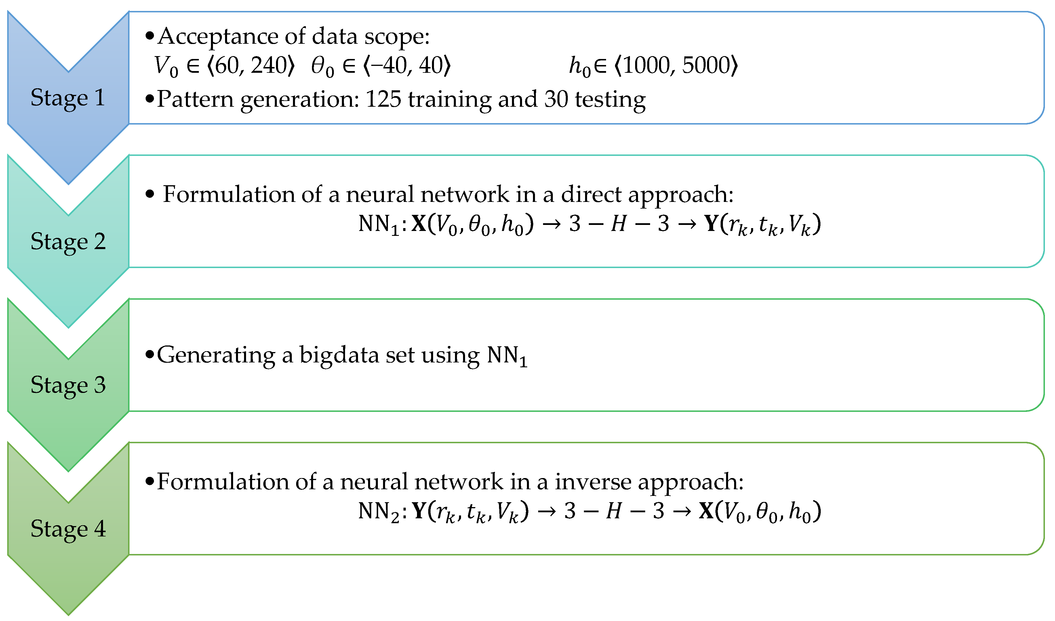
Figure 2.
Trajectories, references systems and external forces acting on the air-dropped capsule.
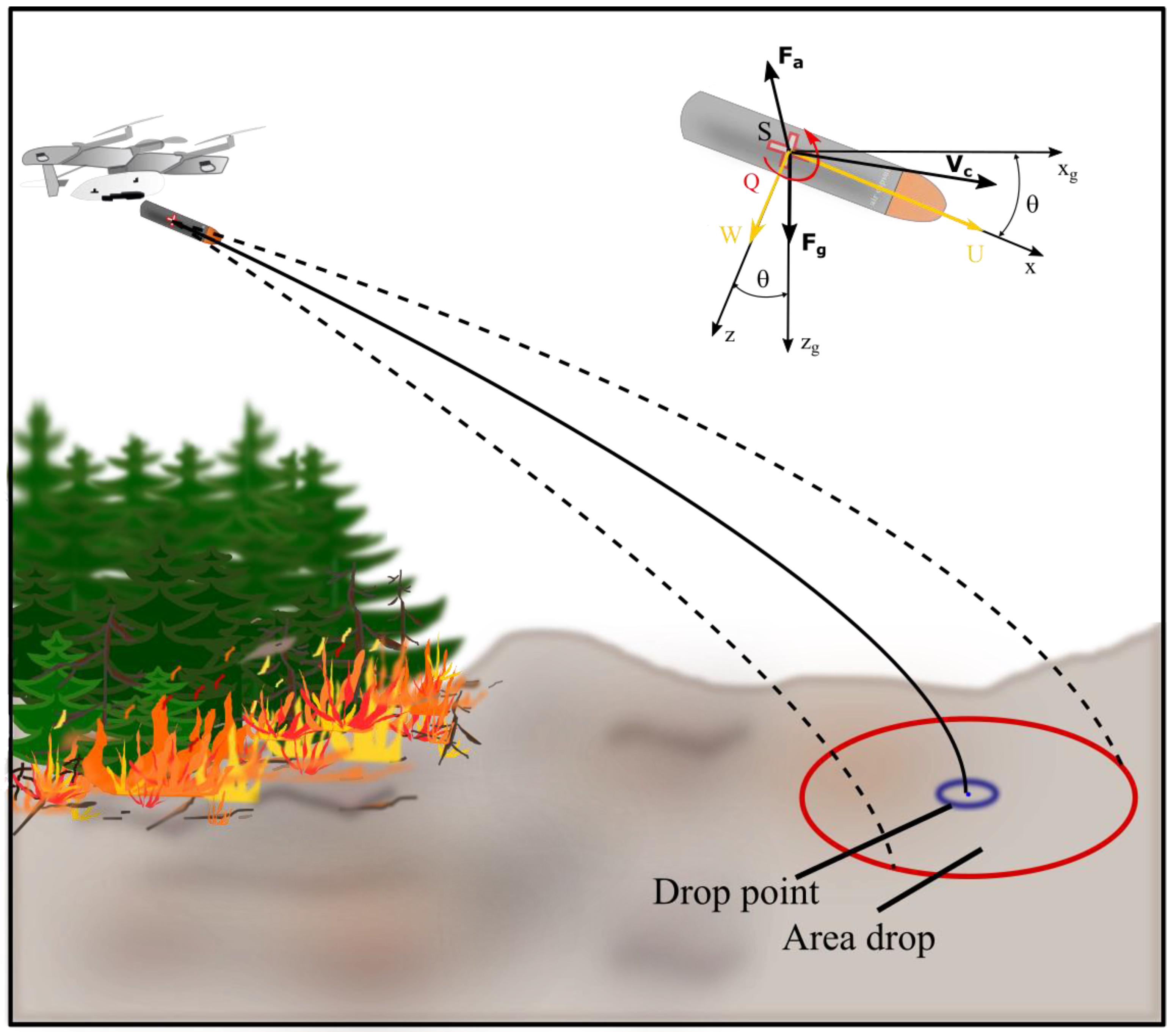
Figure 3.
Visualization of the structure of the reference dataset: scatter plots illustrating the dependency of output variables (rk, tk, Vk) on each of the input parameters (V0, θ0, h0).
Figure 3.
Visualization of the structure of the reference dataset: scatter plots illustrating the dependency of output variables (rk, tk, Vk) on each of the input parameters (V0, θ0, h0).
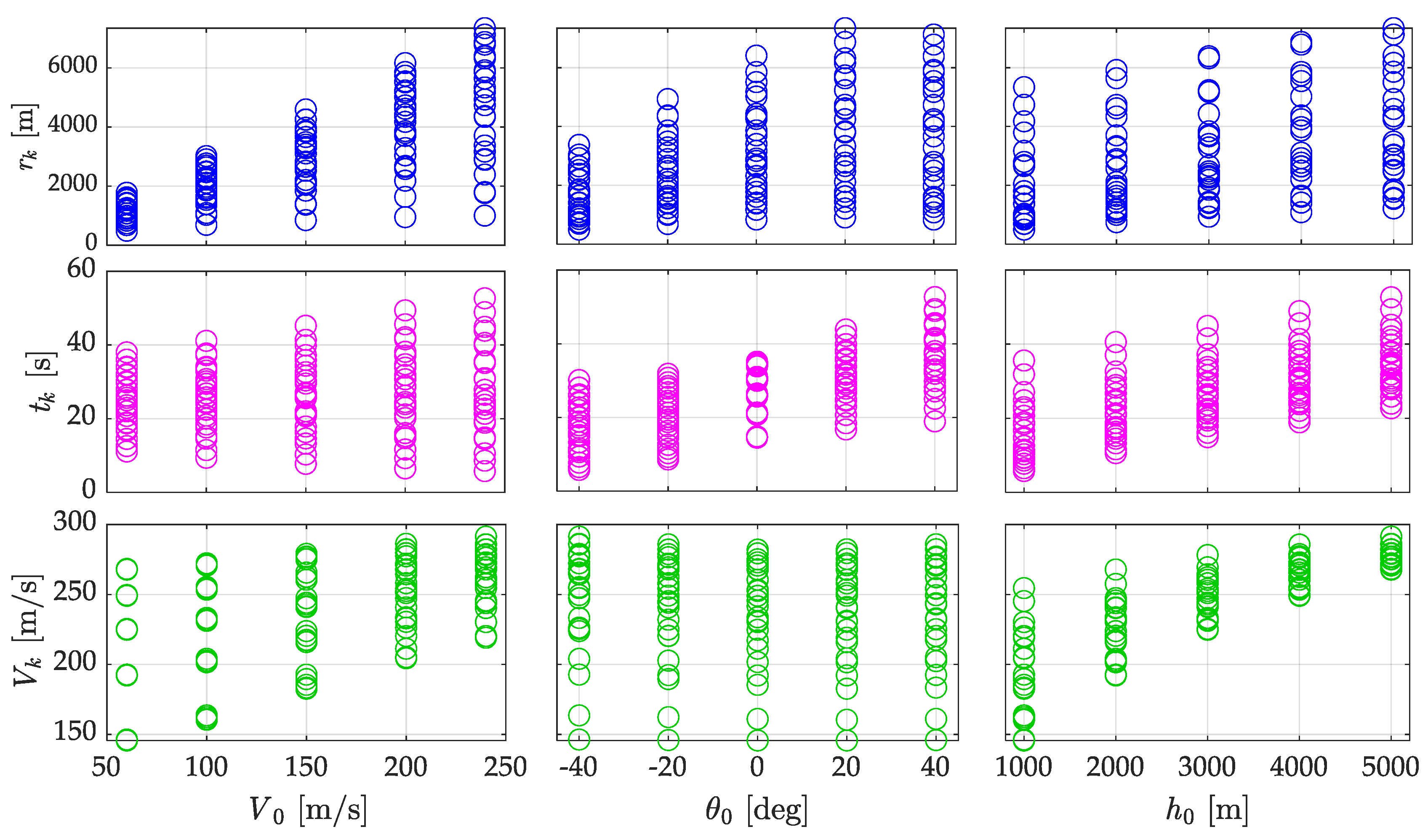
Figure 4.
Structure of NN1.
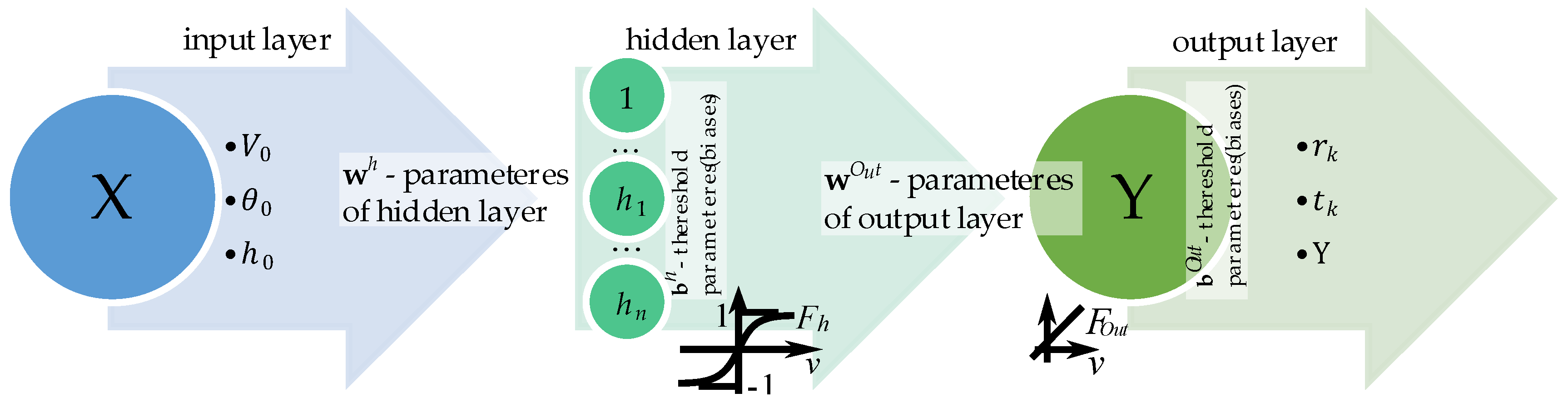
Figure 5.
Mapping of the output variable rk as a function of V0 and θ0, comparing reference data and NN1-generated data.
Figure 5.
Mapping of the output variable rk as a function of V0 and θ0, comparing reference data and NN1-generated data.
Figure 6.
Structure of NN2.
Figure 7.
Bar plots of the percentage error of NN2, for the individual outputs: a) initial speed V₀, b) drop angle θ0, c) drop height h₀.
Figure 7.
Bar plots of the percentage error of NN2, for the individual outputs: a) initial speed V₀, b) drop angle θ0, c) drop height h₀.
Figure 8.
Initial speed V0 reference and predicted values.
Figure 9.
Drop angle θ0 reference and predicted values.
Figure 10.
Drop height h0 reference and predicted values.
Figure 11.
Flight range analysis: comparison of random values with reference data and visualization of minimum deviation.
Figure 11.
Flight range analysis: comparison of random values with reference data and visualization of minimum deviation.
Figure 12.
Flight time analysis: comparison of random values with reference data and visualization of minimum deviation.
Figure 12.
Flight time analysis: comparison of random values with reference data and visualization of minimum deviation.
Figure 13.
Fall speed analysis: comparison of random values with reference data and visualization of minimum deviation.
Figure 13.
Fall speed analysis: comparison of random values with reference data and visualization of minimum deviation.
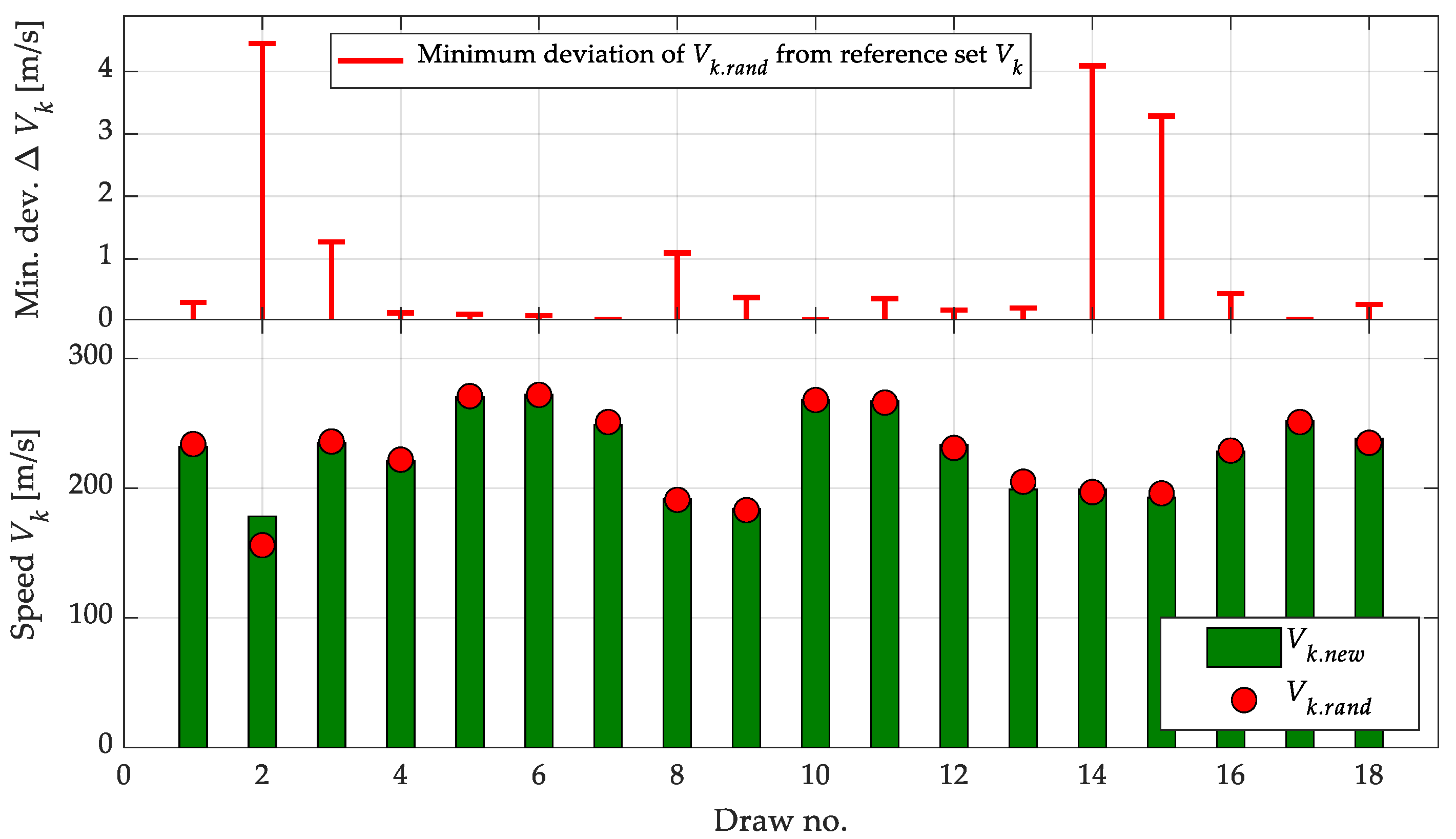

Table 1.
Reference set of 125 data.
| Adopted values | Range | Computed values | Range |
|---|---|---|---|
| [m/s] | [m] | ||
| [deg] | [s] | ||
| [m] | [m/s] |
1 The adopted values were divided into 4 ranges.
Table 2.
Prepared learning and testing data.
| Values | Range | Scale factor | New range |
|---|---|---|---|
| [m/s] | ⟨60, 240⟩ | 252.0 | |
| [deg] | ⟨-40, 40⟩ | 42.0 | |
| [m] | ⟨1000, 5000⟩ | 5250.0 | |
| [m] | ⟨492.8, 734.4⟩ | 7713.7 | |
| [s] | ⟨5.75, 52.68⟩ | 55.3 | |
| [m/s] | ⟨145.62, 291.38⟩ | 305.9 |
Table 3.
MPE and MSE in learning and testing phase of NN1.
| Learning phase | Testing phase | |||
|---|---|---|---|---|
| Values | MPE [%] | MSE | MPE [%] | MSE |
| [m] | 2.03 | 0.0000560 | 2.01 | 0.0000518 |
| [s] | 1.14 | 0.0000331 | 1.30 | 0.0324275 |
| [m/s] | 0.68 | 0.0000421 | 0.63 | 0.1926063 |
Table 4.
MPE, maxPE and MSE in Stage 4.
| Learning phase | |||
|---|---|---|---|
| Values | MPE [%] | maxPE [%] | MSE |
| [m/s] | 0.96 | 7.67 | 0.00002 |
| [deg] | 2.68 | 75.01 | 0.00006 |
| [m] | 0.88 | 10.62 | 0.00001 |
Table 5.
Calculation procedure and error analysis for Case 1.
| Set No. | Variable (A) V0 [m/s] θ0 [deg] h0 [m] |
Stage 1 Output Input to Stage 4 rk [m] tk [s] Vk [m/s] |
Stage 4 Output (B) V0.NN [m/s] θ0.NN [deg] h0.NN [m] |
Percent Error (A−B) [%] |
|---|---|---|---|---|
| 1 (7) | 150.00 -30.00 1500.00 |
1450.20 11.89 207.85 |
150.05 -29.07 1440.27 |
0.03 3.10 3.98 |
| 2 (39) | 150.00 -40.00 2000.00 |
1413.30 13.23 223.83 |
150.93 -39.66 1943.17 |
0.62 0.85 2.84 |
| 3 (59) | 100.00 -20.00 2000.00 |
1538.50 17.61 202.70 |
101.43 -22.89 2102.53 |
1.43 14.47 5.13 |
| 4 (77) | 240.00 -20.00 5000.00 |
4934.00 27.83 285.84 |
236.01 -20.71 4992.56 |
1.66 3.53 0.15 |
| 5 (95) | 200.00 0 3000.00 |
4432.50 26.25 252.51 |
203.75 1.65 2851.01 |
1.88 - 4.97 |
| 6 (123) | 240.00 20.00 1000.00 |
4738.80 24.86 219.08 |
231.50 20.84 1061.39 |
3.54 4.19 6.14 |
Table 6.
Range: random values vs. new reference values and deviation analysis.
| Draw No. | Input to Stage 4 (C): rk.rand [m] |
Stage 1 Result (D): rk.new [m] | Percent Error (C−D) [%] | Absolute Error (C−D) [m] |
Min. Dev. of Δrk [m] |
|---|---|---|---|---|---|
| 1 | 4213.00 | 4205.10 | 0.19 | 7.90 | 35.30 |
| 2 | 2692.00 | 2569.70 | 4.76 | 122.30 | 4.10 |
| 3 | 3504.00 | 3436.00 | 1.98 | 68.00 | 17.40 |
| 4 | 2257.00 | 2319.0 | 2.67 | 62.00 | 7.20 |
| 5 | 3567.00 | 3907.30 | 8.71 | 340.30 | 80.40 |
| 6 | 2966.00 | 3064.90 | 3.23 | 98.90 | 44.00 |
| 7 | 3353.00 | 3344.80 | 0.25 | 8.20 | 21.00 |
| 8 | 1925.00 | 2108.80 | 8.72 | 183.80 | 6.00 |
| 9 | 755.00 | 797.27 | 5.30 | 42.27 | 11.37 |
| 10 | 3067.00 | 3132.80 | 2.10 | 65.80 | 24.80 |
| 11 | 6647.00 | 6731.70 | 1.26 | 84.67 | 139.90 |
| 12 | 3309.00 | 3238.90 | 2.16 | 70.10 | 11.50 |
| 13 | 2636.00 | 2460.00 | 7.15 | 176.00 | 1.30 |
| 14 | 705.00 | 776.87 | 9.25 | 71.87 | 12.99 |
| 15 | 1453.00 | 1431.80 | 1.48 | 21.20 | 2.80 |
| 16 | 5191.00 | 5185.10 | 0.11 | 5.90 | 6.90 |
| 17 | 5921.00 | 5988.70 | 1.13 | 67.70 | 0.50 |
| 18 | 6334.00 | 5597.10 | 13.17 | 736.90 | 11.70 |
Table 7.
Flight time: random values vs. new reference values and deviation analysis.
| Draw No. | Input to Stage 4 (C): tk.rand [s] |
Stage 1 Result (D): tk.new [s] |
Percent Error (C−D) [%] |
Absolute Error (C−D) [s] | Min. Dev. of Δtk [s] |
|---|---|---|---|---|---|
| 1 | 26.00 | 25.86 | 0.54 | 0.14 | 0.010 |
| 2 | 18.00 | 23.35 | 22.91 | 5.35 | 0.145 |
| 3 | 33.00 | 33.11 | 0.33 | 0.11 | 0.048 |
| 4 | 15.00 | 15.00 | 0 | 0 | 0.114 |
| 5 | 48.00 | 44.94 | 6.81 | 3.06 | 0.924 |
| 6 | 41.00 | 41.13 | 0.32 | 0.13 | 0.133 |
| 7 | 38.00 | 37.65 | 0.93 | 0.35 | 0.001 |
| 8 | 42.00 | 29.28 | 43.44 | 12.72 | 0.121 |
| 9 | 14.00 | 14.26 | 1.82 | 0.26 | 0.241 |
| 10 | 36.00 | 36.37 | 1.02 | 0.37 | 0.018 |
| 11 | 41.00 | 40.96 | 0.10 | 0.04 | 0.133 |
| 12 | 17.00 | 16.45 | 3.34 | 0.55 | 0.080 |
| 13 | 31.00 | 30.20 | 2.65 | 0.80 | 0.005 |
| 14 | 17.00 | 17.23 | 1.33 | 0.23 | 0.080 |
| 15 | 12.00 | 11.90 | 0.84 | 0.10 | 0.114 |
| 16 | 33.00 | 34.05 | 3.08 | 1.05 | 0.048 |
| 17 | 38.00 | 38.99 | 2.54 | 0.99 | 0.001 |
| 18 | 48.00 | 38.93 | 23.30 | 9.07 | 0.924 |
Table 8.
Final descent velocity: random values vs. new reference values and deviation analysis.
| Draw No. | Input to Stage 4 (C): Vk.rand [m/s] |
Stage 1 Result (D): Vk.new [m/s] |
Percent Error (C−D) [%] |
Absolute Error (C−D) [m/s] |
Min. Dev. of ΔVk [m/s] |
|---|---|---|---|---|---|
| 1 | 234.00 | 231.88 | 0.91 | 2.12 | 0.30 |
| 2 | 156.00 | 178.19 | 12.45 | 22.19 | 4.45 |
| 3 | 236.00 | 235.15 | 0.36 | 0.85 | 1.27 |
| 4 | 222.00 | 220.97 | 0.47 | 1.03 | 0.13 |
| 5 | 271.00 | 270.37 | 0.23 | 0.63 | 0.11 |
| 6 | 272.00 | 272.33 | 0.12 | 0.33 | 0.09 |
| 7 | 251.00 | 248.95 | 0.82 | 2.05 | 0.03 |
| 8 | 191.00 | 191.81 | 0.42 | 0.81 | 1.09 |
| 9 | 183.00 | 184.06 | 0.58 | 1.06 | 0.38 |
| 10 | 268.00 | 268.18 | 0.07 | 0.18 | 0.02 |
| 11 | 266.00 | 267.33 | 0.50 | 1.33 | 0.36 |
| 12 | 231.00 | 233.47 | 1.06 | 2.47 | 0.18 |
| 13 | 205.00 | 199.00 | 3.02 | 6.00 | 0.21 |
| 14 | 197.00 | 198.95 | 0.98 | 1.95 | 4.09 |
| 15 | 196.00 | 192.70 | 1.71 | 3.30 | 3.28 |
| 16 | 229.00 | 228.33 | 0.29 | 0.67 | 0.44 |
| 17 | 251.00 | 252.26 | 0.50 | 1.26 | 0.03 |
| 18 | 235.00 | 238.14 | 1.32 | 3.14 | 0.27 |
Table 9.
Baseline flight parameters determined by the NN2 network.
| Draw No. | V0.NN [m/s] | θ0.NN [°] | h0.NN [m] |
|---|---|---|---|
| 1 | 192.53 | 11.22 | 2126.03 |
| 2 | 140.17 | 30.44 | 1000.00 |
| 3 | 138.71 | 30.62 | 2816.64 |
| 4 | 174.76 | -15.08 | 1663.18 |
| 5 | 153.44 | 46.80 | 4399.42 |
| 6 | 108.77 | 36.14 | 4993.07 |
| 7 | 133.79 | 39.46 | 3442.67 |
| 8 | 119.64 | 48.61 | 1540.09 |
| 9 | 78.36 | -41.24 | 1656.65 |
| 10 | 105.05 | 16.01 | 4797.22 |
| 11 | 237.73 | 26.25 | 3582.56 |
| 12 | 222.36 | -4.50 | 1480.92 |
| 13 | 130.14 | 45.96 | 1610.60 |
| 14 | 66.26 | -43.64 | 2127.58 |
| 15 | 138.07 | -22.62 | 1263.42 |
| 16 | 220.27 | 33.28 | 1625.57 |
| 17 | 226.62 | 31.75 | 2703.74 |
| 18 | 231.41 | 39.59 | 1847.37 |
Disclaimer/Publisher’s Note: The statements, opinions and data contained in all publications are solely those of the individual author(s) and contributor(s) and not of MDPI and/or the editor(s). MDPI and/or the editor(s) disclaim responsibility for any injury to people or property resulting from any ideas, methods, instructions or products referred to in the content. |
© 2025 by the authors. Licensee MDPI, Basel, Switzerland. This article is an open access article distributed under the terms and conditions of the Creative Commons Attribution (CC BY) license (http://creativecommons.org/licenses/by/4.0/).
Copyright: This open access article is published under a Creative Commons CC BY 4.0 license, which permit the free download, distribution, and reuse, provided that the author and preprint are cited in any reuse.


