Submitted:
29 August 2025
Posted:
02 September 2025
Read the latest preprint version here
Abstract
Meta-analysis has become central to evidence-based medicine, yet a persistent gap remains between statistical experts and clinicians in understanding the implications of model choice. The distinction between fixed- and random-effects is often dismissed as a technical detail, when in fact it defines the very philosophy of evidence synthesis and must be addressed conceptually, a priori, rather than dictated by heterogeneity statistics. Fixed-effect models convey the illusion of a single universal truth, offering apparent precision but resting on an assumption rarely met in clinical practice. Random-effects models, by contrast, acknowledge that true effects differ across studies, populations, and settings, providing wider but more credible intervals that reflect real-world diversity. This work presents a tutorial designed to explain, in a simple and accessible manner, how to conduct an updated and robust evidence synthesis. Through real and simulated examples—including clinical scenarios, a worked hypothetical meta-analysis, re-analyses of published reviews, and the metaphor of body temperature—the tutorial demonstrates how model choice can fundamentally alter conclusions. Results that appear significant under a fixed-effect model may become non-significant with more robust random-effects methods, due to wider confidence intervals that account for between-study heterogeneity. In contrast, prediction intervals reveal the range of effects likely to be observed in practice. Drawing on Cochrane guidance, the discussion highlights current standards, including REML and Paule–Mandel estimators, Hartung–Knapp–Sidik–Jonkman confidence intervals, and the routine use of prediction intervals. By combining intuitive analogies with practical applications, the tutorial provides clinicians with an accessible introduction to contemporary meta-analytic methods, promoting more reliable evidence synthesis.
Keywords:
meta-analysis
; fixed-effect model
; random-effects model
; heterogeneity
; evidence synthesis
; Cochrane Handbook
Introduction
Two meta-analyses, based on the very same set of studies, may yield strikingly different conclusions. For the clinician reviewing the literature, this contradiction is more than a statistical curiosity—it is a source of genuine confusion that can shape clinical decisions. Why does this happen? More often than not, the explanation lies in a modeling choice rarely discussed outside statistical circles: whether the analysis was conducted under a fixed-effect or a random-effects framework.
This choice is not a technical footnote. It determines whether a meta-analysis communicates the illusion of a single universal truth or the reality of variable effects across diverse settings.
In practical terms, it is the difference between reporting a highly precise estimate that assumes all studies are interchangeable and presenting a more cautious summary that acknowledges heterogeneity as part of clinical reality—a distinction often misunderstood in clinical research [1]. Not only are such heterogeneity statistics misused to dictate model choice, but doing so confuses cause and effect: model philosophy should be set conceptually a priori, not driven by an I² value.
For clinicians, understanding this distinction is essential. It reframes meta-analysis not as a machine for producing a single “answer,” but as a tool for interpreting variability in evidence. In this article, we offer a foundational explanation of fixed versus random effects, using a familiar clinical metaphor to make the concepts intuitive. This work aims not only to clarify statistical modeling but also to demonstrate why model choice carries direct consequences for how evidence is translated into practice.
The Foundational Question: One True Effect?
At its heart, the choice of model boils down to this: do we believe that every study is measuring the same single effect, or do we accept that true effects differ from one study to another? [2]
The fixed-effect model assumes the former. It treats each study as a repeated measurement of the same underlying truth, with differences explained solely by chance. In this view, there is one “true effect,” and the task of meta-analysis is to identify it with the greatest possible precision.
The random-effects model assumes the latter. It acknowledges that effects may legitimately differ across settings, populations, and methods. Rather than assuming one universal truth, it estimates the average of a distribution of true effects and incorporates that variability into the pooled estimate [3].
A clinical metaphor illustrates the distinction. Consider human body temperature:
- Under a fixed-effect view, we would insist that the true temperature is always 37.0 °C. Any deviation measured in practice—36.8 °C, 37.3 °C—would be dismissed as random error around this single correct value.
- Under a random-effects view, we recognize that normal body temperature is not identical for everyone. Some individuals average 36.5 °C, while others average 37.2 °C, and variations also occur with time of day, measurement method, or physiological state. There is still a meaningful average around 37 °C, but it represents a summary of genuine diversity rather than an immutable truth.
This metaphor captures the essence of fixed versus random effects: one offers the illusion of uniformity, the other reflects the reality of variability. Choosing between them is not just a statistical decision—it determines whether we present evidence as a single number or as a distribution that mirrors clinical practice. Just as an individual’s temperature can vary yet still be normal, in meta-analysis a treatment’s effect can vary across studies yet still be real. Importantly, clinical effects often exhibit even greater variability than body temperature—sometimes differing not only in magnitude but also in direction.
While the body temperature metaphor effectively illustrates the contrast between a single value and a distribution, it is worth noting that clinical treatment effects can exhibit far wider variability. In some cases, results may not only differ in magnitude but even cross the null—showing benefit in certain contexts and possible harm in others. This broader spectrum of heterogeneity goes beyond the relatively narrow physiological range of normal temperature, but the metaphor remains useful as an entry point to the concept. This distinction is critical: while a fluctuation between 36.5 °C and 37.2 °C carries little clinical consequence, the variability of treatment effects can extend from meaningful benefit to genuine harm. In this sense, the stakes of heterogeneity in clinical research are far higher than in physiology, making the recognition of treatment-effect distributions a matter of patient safety and health policy.
Table 1 provides additional clinical examples that illustrate how fixed- and random-effects models embody fundamentally different assumptions, leading to distinct interpretations of the same evidence.
Fixed-Effect: Clarity with a Cost
The appeal of the fixed-effect model lies in its apparent simplicity. By treating every study as a replicate of the same underlying truth, it produces a single pooled estimate with narrow confidence intervals. To the busy clinician, this precision can be seductive: it seems to promise certainty.
Yet this clarity comes at a cost. If true effects genuinely differ across settings, the fixed-effect approach erases that variability, presenting heterogeneity as if it were mere random noise. The result is an artificially precise number that risks overstating the generalizability of the evidence.
Returning to our metaphor of body temperature, the fixed-effect model insists that the true temperature of a human being is exactly 37.0 °C. A reading of 36.7 °C or 37.3 °C is treated only as a measurement error. Clinically, however, we know that variation in normal body temperature is real, not illusory.
A practical example illustrates the point. As shown in Table 1, a fixed-effect model assumes, for instance, that screening colonoscopy reduces colorectal cancer mortality by the same amount everywhere, or that ACE inhibitors lower blood pressure identically in all patients. Such pooling yields a deceptively precise number, but one that obscures real differences driven by program quality, patient characteristics, or adherence. Importantly, this cost is not merely a loss of realism but a quantifiable statistical bias: when the assumption of homogeneity is violated, fixed-effect models yield biased significance tests and misleadingly narrow confidence intervals. Evidence from large-scale re-analyses supports this concern.
In short, fixed-effect analysis can create the mirage of certainty: an attractive single number that conceals rather than reflects clinical diversity. Although there are rare situations where a fixed-effect approach may be justified—such as highly homogeneous studies or sensitivity analyses—it should not be the default choice in clinical meta-analysis, where acknowledging variability is almost always the more appropriate stance.
Random-Effects: Embracing Variability
In contrast, the random-effects model begins from a different premise: that variation across studies is not merely noise, but often reflects genuine differences between them. These differences may arise from multiple sources—such as populations, clinical settings, or how an intervention is implemented. Instead of forcing all studies into a single truth, the random-effects model estimates the mean of a distribution of true effects and widens the confidence interval to reflect that diversity.
Returning to our body temperature metaphor, the random-effects model accepts that normal temperature does not have to be exactly 37.0 °C. Some people run at 36.5 °C, others at 37.2 °C. These differences are real, influenced by factors such as genetics, race, age, time of day, or even the measurement method used. The pooled value around 37 °C is still useful, but only when understood as an average of many true values, not as a universal constant.
Clinically, this perspective is more faithful to reality. As shown in Table 1, the benefit of screening colonoscopy may be greater in well-resourced, high-coverage programs and smaller in under-resourced settings. The blood-pressure response to ACE inhibitors differs across patient groups, shaped by comorbidity, adherence, baseline risk, and even race. Random-effects models explicitly incorporate such heterogeneity into the summary estimate.
The price to pay is less apparent precision. Confidence intervals under random-effects are usually wider. Put simply, a confidence interval is the range of values within which the true effect is most likely to lie. A narrow interval may look more reassuring, but if it ignores genuine variation, it can be misleading. Wider intervals under random-effects are not a weakness—they are a more honest reflection of the uncertainty clinicians face when applying evidence across diverse contexts.
In practice, random-effects analysis acknowledges what every clinician already knows: patients, hospitals, and health systems are not identical. By embracing variability, it avoids the illusion of false certainty and produces estimates that more accurately reflect the realities of real-world medicine.
Methodological Choices within the Random-Effects Framework
Random-effects analysis is not a single recipe. There are different ways to estimate the average effect and its uncertainty, and the choice can influence the final numbers. Two aspects matter most: how we estimate the amount of heterogeneity (the model) and how we calculate the confidence interval (the CI method).
1. Estimating heterogeneity (“the model”): All random-effects models try to capture how much the true effects vary between studies, but they use different formulas to do it.
- DerSimonian–Laird (DL): the classic method, fast and simple, but tends to underestimate variability (i.e., the real differences between study results) when there are few studies. This underestimation can result in overly narrow confidence intervals, thereby increasing the risk of false-positive findings (especially in meta-analyses with a small number of studies) [4]. This method persists because it is the long-standing default in many software packages.
- Paule–Mandel (PM): another robust option, often recommended today as an alternative to DL, particularly when heterogeneity is moderate. It has been endorsed in the Cochrane Handbook and supported by comparative evaluations [6].
2. Calculating confidence intervals (“the CI”): Once the average effect is estimated, we need to decide how wide the confidence interval should be.
- Wald CI: the traditional, straightforward approach; it often produces intervals that look reassuringly precise but can be too narrow, especially when there are few studies or some heterogeneity [2].
- Hartung–Knapp–Sidik–Jonkman (HKSJ): a modern method that produces wider and generally more reliable intervals. It is now considered the standard when heterogeneity is present. With very few studies, it can sometimes yield excessively wide (over-conservative) intervals; however, it remains the better option overall, as cautious inference is safer than overconfident conclusions [7,8].
- Modified or truncated HKSJ (mHK): a refinement of the HKSJ method, designed to prevent confidence intervals from becoming excessively wide in rare situations—typically when the number of studies is very small, a common scenario in clinical research, or when the between-study variance is close to zero [9].
Random-effects models all share the same philosophy—accepting variability—but they differ in how cautious they are. DL + Wald often looks neat and “precise” but can be misleading. REML or Paule–Mandel combined with HKSJ intervals are increasingly seen as the safer choices when evidence is sparse or heterogeneous [2].
Heterogeneity as the Compass for Model Choice
What Heterogeneity Means
Heterogeneity means that the results of studies are not identical [10,11,12,13]. Sometimes this variation is small and trivial; other times it is significant and clinically meaningful. In meta-analysis, the question is not whether differences exist—they almost always do—but whether we interpret them as noise around one truth or as signals of genuinely different effects.
Clinical vs. Statistical Heterogeneity
Two forms of heterogeneity should be distinguished:
- Clinical heterogeneity: This is the real-world variability we expect when studies are not identical in who they include, what they do, or where they are done. Patients may differ in age, comorbidities, or disease severity; interventions may vary in dose, surgical technique, or how strictly protocols are followed; and settings may range from highly specialized hospitals to resource-limited clinics. These differences are not errors but part of normal clinical diversity—and they often explain why study results do not all look the same.
- Statistical heterogeneity: this is heterogeneity “put into numbers.” It describes how much the results of the included studies differ once we account for normal random fluctuations due to sample size. Every study will vary slightly, simply due to chance—this is known as sampling error. However, when the differences are greater than what chance alone would explain, we refer to it as statistical heterogeneity. Indices like Q, I², and τ² are simply ways of expressing that variability in numbers.
Model Choice Should Come First (and I² Should not Be Used to Make This Choice)
Crucially, the decision between fixed- and random-effects models must be made conceptually before looking at any statistics [2]. The choice rests on whether we believe in a single universal effect or in a distribution of effects shaped by context. Measures of heterogeneity are helpful descriptors, but they do not dictate the model's philosophy.
Statistical heterogeneity refers to the variability observed when combining study results, beyond what would be expected from random sampling error alone. Indices such as Q, I², and τ² quantify this variability [6,10,11,12], but they should be interpreted as guides to the extent of differences, not as arbiters of which model to use. As we will emphasize later, selecting between fixed and random effects purely based on I² is misguided: the underlying conceptual question is whether one effect or many?—must always come first.
Measuring Statistical Heterogeneity
There are several common tools, each with a distinct role:
- Cochran’s Q: a test that asks whether the differences between studies are greater than expected by chance [10]. Its main limitation is that it strongly depends on the number of studies: with few, it often misses real differences; with many, it flags even trivial ones. A non-significant Q should therefore never be taken as proof of homogeneity.
- I²: the percentage of total variation explained by real heterogeneity rather than chance. Values of 25%, 50%, and 75% are often described as low, moderate, and high heterogeneity, though thresholds are arbitrary [11,12]. Moreover, I² itself is only an estimate and carries considerable uncertainty, particularly when the number of studies is small. It is also strongly influenced by the precision of the included studies: meta-analyses with large sample sizes can yield high I² values even when the absolute differences in effects are clinically trivial. These limitations further reinforce why model choice should be made conceptually rather than dictated by I².
- τ² (between-study variance): measures how much the true effects differ across studies. It is reported on the same scale as the effect size (e.g., risk difference in absolute %, or log scale for risk ratios). A τ² of 0 means no variability at all [2,6]. An estimated τ² of 0 suggests that there is no evidence of between-study variance beyond what would be expected by chance. τ² matters because it drives the weights in a random-effects model and is essential for calculating prediction intervals [2,6].
Putting it Together
In practice, heterogeneity is expected in almost every clinical question. The key is not whether it exists, but what it means. If studies are highly consistent, fixed- and random-effects estimates converge. If studies diverge, random-effects models acknowledge that reality, whereas fixed-effect models may suppress it.
The Guiding Role of Heterogeneity
Heterogeneity is thus not a flaw to be eliminated, but a compass: it helps us interpret the evidence and understand when variability matters. By embracing it, meta-analysis shifts from delivering a single, over-simplified answer to providing a more nuanced picture of reality—one that clinicians can trust when applying results to diverse patients and settings. Returning to our metaphor, heterogeneity in meta-analysis is no different from the spread of normal body temperatures: expected, natural, and informative when properly understood.
Prediction Intervals: Looking Beyond Confidence Intervals
Confidence intervals (CIs) around the pooled effect describe the precision of the average estimate. However, clinicians are often less interested in the mean effect and more concerned with what might happen in their own setting. For this purpose, prediction intervals (PIs) are more informative: they estimate the range within which the true effect of a new study, in a comparable context, is expected to fall [3,14,15]. Most importantly, PIs often expose the fragility of apparently significant findings. In large-scale reanalysis, almost 75% of statistically significant meta-analyses had PIs including the null [16].
Returning to our body temperature metaphor, the average human temperature may be 37.0 °C, and a 95% CI around the mean might be 36.9–37.1 °C. This interval is very narrow—but it only tells us how precisely we know the mean. A PI, in contrast, reflects the actual spread of normal body temperatures (e.g., 36.5–37.5 °C). This is directly linked to τ², which quantifies the between-study variance (τ²): the larger τ², the wider the prediction interval. This width is not arbitrary; the PI is calculated directly from the τ². A large τ² mathematically guarantees a wide PI. In our metaphor, τ² is the statistical estimate of how much temperatures vary across the studies we have in hand, while the prediction interval (e.g., 36.5–37.5 °C) conveys the range we would expect to observe in new or future patients.
Clinically, this distinction is crucial. A confidence interval might suggest that the effect of screening colonoscopy is “precisely” a 20% reduction in mortality, but the prediction interval may reveal that in some contexts, the effect is close to 40%, while in others, it approaches zero. By reporting both CIs and PIs, meta-analyses can move from abstract averages to a more realistic picture of how results may vary across real-world settings. Therefore, when counseling a patient or developing a local protocol, the prediction interval—when available—provides a more realistic and clinically relevant range of potential outcomes than the confidence interval alone. For example, when communicating results, a clinician might say: ‘Across all studies, the average benefit of this treatment was about a 20% reduction in risk (as reflected by the confidence interval). However, the prediction interval indicates that in a specific future setting, the effect could plausibly range from a 40% reduction to no benefit at all. This wider range provides a more realistic expectation of how the treatment might perform in our own patient population
So, Which Model Should I Choose?
Key Principles for Model Choice
The decision between fixed- and random-effects is not a technical footnote—it reflects how we understand the evidence. Fixed-effect assumes that there is a single underlying effect that applies everywhere. Random-effects models, by contrast, assume that true effects differ across studies, shaped by patient characteristics, interventions, and contexts. In medicine, such diversity is the rule, not the exception.
For this reason, model choice should be made conceptually, before looking at any statistics. Numbers like Q, I², or τ² are useful for describing how much studies vary, but they do not determine the philosophy of the model. The starting point must always be the question: do we believe in one effect, or in many? It is the same distinction as asking whether there is one single ‘normal’ temperature or a distribution of normal values across people.
Table 2 summarizes the key criteria that distinguish fixed-effect from random-effects models and guides the use of each when they may be appropriate in clinical meta-analysis.
What Cochrane Recommends
The Cochrane Handbook is explicit on this issue [2]. Random-effects models are generally the safer choice whenever clinical diversity is present—meaning, in most clinical questions. Fixed-effect can be defensible only when studies are virtually identical in design, participants, and context, a situation that is rare outside very narrow questions.
Cochrane also warns against a common mistake: switching between models based on whether I² is “high” or “low.” Heterogeneity statistics describe variability, but they should not dictate the model. Instead, the model should be chosen a priori, guided by the plausibility of one universal effect versus a distribution of effects. Increasingly, Cochrane reviews present both: random-effects as the main analysis, and fixed-effect as a sensitivity check.
Table 3 reports the explicit recommendations of the Cochrane Handbook on model choice and inference, together with their practical implications for clinical meta-analysis.
Practical Guidance for Clinicians
For clinicians interpreting meta-analyses, several practical lessons can be drawn. Random-effects should usually be the default, because patients and hospitals are not interchangeable. Fixed-effect has a role, but mainly as a sensitivity analysis or in narrowly defined questions where studies are genuinely homogeneous.
Statistical significance under fixed-effect should not be mistaken for robustness. If a result disappears when random effects are applied, that is a warning sign that variability matters and the evidence is fragile. Finally, always look at the forest plot before the summary number. If studies point in different directions, an apparently precise fixed-effect estimate is misleading. Just as a single thermometer reading can miss the natural variability across individuals, a single fixed-effect estimate can obscure meaningful differences between studies.
Making it Visual: Fixed vs Random at a Glance
The contrast between fixed- and random-effects models is not only conceptual but also readily visible. Figure 1 presents, for illustrative purposes, a simulated meta-analysis of six randomized trials evaluating a hypothetical new antithrombotic agent for the prevention of postoperative thrombosis. Each trial compared the novel drug with conventional prophylaxis, reporting the number of thrombotic events in each group. While all studies suggested fewer events in the treatment arm, the magnitude of benefit varied substantially across trials.
Under a fixed-effect Mantel–Haenszel model (a fixed-effect pooling method), pooling the six studies yielded a statistically significant reduction in thrombotic events with narrow confidence intervals (RR 0.73, 95% CI 0.62–0.87; p<0.01). At face value, this implies that the new antithrombotic reduces postoperative thrombosis by roughly 27% in every surgical context. However, when a random-effects model with REML estimation was applied, the pooled effect remained directionally similar but the confidence interval widened (RR 0.76, 95% CI 0.58–0.99; p = 0.04). Incorporating the Hartung–Knapp adjustment further broadened the interval, rendering the result statistically non-significant (RR 0.76, 95% CI 0.55–1.05; p = 0.08).
Most importantly, the prediction interval revealed the fragility of the evidence: in a future trial, the true effect could plausibly range from a 64% risk reduction to a 57% risk increase (95% PI 0.36–1.57). In other words, while some surgical populations might experience substantial benefit, others could see little to no advantage—or even possible harm. With moderate heterogeneity (I² = 50.77%, Q = 10.96, p = 0.05, τ² = 0.05), this example underscores how fixed-effect analysis may create the illusion of a universal benefit, whereas random-effects modelling more faithfully represents the uncertainty and variability encountered in clinical practice.
The heterogeneity observed in this example could plausibly arise from multiple sources: Do all patients across trials share the same baseline thrombotic risk, or were study populations selected differently? Were thrombotic events documented consistently across centers, or did outcome assessment vary? Were prophylaxis protocols strictly adhered to in all trials, or was implementation uneven? These questions illustrate that heterogeneity is not a nuisance but often reflects genuine clinical and methodological differences that need to be acknowledged rather than averaged away.
How to Report a Meta-Analysis
Methods
Transparency in methods is essential. A well-reported meta-analysis should clearly state which statistical model was used (fixed- or random-effects, with the specific estimator such as DerSimonian–Laird, Paule–Mandel, or REML), the software and commands employed, and the planned strategies to explore heterogeneity. This includes pre-specified subgroup analyses (e.g., by population, setting, or intervention dose), sensitivity analyses (e.g., excluding high-risk-of-bias studies), and, when appropriate, meta-regression. Any continuity corrections (adjustments for studies with zero events in one arm) should be explicitly described, as different corrections can yield different results. By laying out these choices in advance, the analysis avoids the perception of selective reporting and allows full reproducibility. Continuing with our metaphor, report not only the mean body temperature (37 °C), but also the normal spread (for example, 36.5–37.5 °C), as both are important for interpretation. Equally important, meta-analyses should adhere rigorously to established methodological standards. The Cochrane Handbook for Systematic Reviews of Interventions provides detailed guidance on appropriate model selection, heterogeneity assessment, and sensitivity analyses [2], while the PRISMA 2020 statement ensures transparent and complete reporting of methods and results [17]. Following these frameworks not only strengthens methodological rigor but also facilitates critical appraisal, reproducibility, and trust in the evidence synthesized.
Results
In the results section, findings should be presented with forest plots that are legible and fully annotated, showing study-level estimates, pooled effects, and heterogeneity measures (Q, I², τ²). Both confidence intervals (CI) and, when possible, prediction intervals (PI) should be reported to convey not only the precision of the mean effect but also the likely range of effects in future settings. The type of model and interval calculation method (e.g., Wald vs. Hartung–Knapp–Sidik–Jonkman) must be specified, since some software packages (such as CMA) provide only default or limited options. If continuity corrections were applied, these must also be reported, with justification for the chosen method. Above all, the principle of maximum transparency is paramount: every analytical choice should be transparent to the reader, ensuring that conclusions are seen as robust and reproducible.
Table 4 summarizes the essential elements that should be transparently reported in the methods and results of a meta-analysis, including model choice, heterogeneity measures, confidence and prediction intervals, and sensitivity analyses.
Real-World Case Studies: How Fixed vs Random-Effects Alter Conclusions
Applied case study 1: Urination stimulation techniques in infants
Clean urine collection in non-toilet-trained infants is clinically challenging: invasive methods, such as suprapubic aspiration, are painful, while non-invasive alternatives, like urine bags, are prone to contamination. Recently developed stimulation techniques (e.g., Herreros’ tapping/massage and the Quick-Wee cold gauze method) aim to facilitate voiding in infants under one year. The available trials, however, differ in infant age, maneuver applied, clinical setting, and outcome definitions, introducing substantial heterogeneity.
In this context, a published meta-analysis applied a fixed-effect Mantel–Haenszel model, pooling three small randomized trials and reporting a precise and statistically significant effect (OR 3.88, 95% CI 2.28–6.60; p < 0.01; I² = 72%) [18]. This approach assumes identical efficacy across studies, an assumption that may not hold given the clinical diversity. When the data were re-analysed using a random-effects model with REML estimation, the effect remained directionally similar but with wider confidence intervals (OR 3.44, 95% CI 1.20–9.88; p = 0.02). With the Hartung–Knapp–Sidik–Jonkman (HKSJ) adjustment, recommended for small and heterogeneous datasets, the interval widened further and statistical significance was lost (OR 3.44, 95% CI 0.34–34.91; p = 0.15) [19]. This scenario remains partially conflicting: with very few studies, Wald-type intervals tend to be overly optimistic, whereas HKSJ intervals can become excessively conservative. In such cases, the most informative approach is to present both sets of results and interpret them jointly. Nevertheless, this example illustrates how fixed-effect modelling can overstate precision in the presence of variability. In contrast, random-effects methods with robust interval estimation provide a more cautious and clinically faithful interpretation.
Applied case study 2: musculoskeletal outcomes after esophageal atresia repair
Children with esophageal atresia (EA) require surgical repair, most commonly through conventional open thoracotomy repair (COR) or thoracoscopic repair (TR). Long-term musculoskeletal sequelae—such as scoliosis, rib fusion, and scapular winging—are recognized complications, particularly after open procedures involving rib spreading. A recent meta-analysis compared TR with thoracotomy; however, the included studies varied in follow-up duration, diagnostic methods (clinical assessment versus imaging), and surgeon expertise. These differences introduce clinical heterogeneity, making the assumption of a single common effect less plausible.
In this setting, the analysis employed a fixed-effect Mantel–Haenszel model, reporting statistically significant and precise reductions in musculoskeletal complications with TR (e.g., scoliosis: RR 0.35, 95% CI 0.14–0.84; p = 0.02) [20]. With only four small retrospective studies and moderate inconsistency (I² = 38%), a random-effects model using REML estimation yielded wider intervals and reduced certainty (RR 0.35, 95% CI 0.09–1.36; p = 0.13). When the Hartung–Knapp–Sidik–Jonkman (HKSJ) adjustment was applied, the confidence interval broadened further, and statistical significance was lost (RR 0.35, 95% CI 0.05–2.36; p = 0.18) [21].
This case illustrates how fixed-effect modelling can produce narrow intervals that may overstate certainty. In contrast, random-effects approaches, particularly REML with HKSJ adjustment, provide a more cautious and clinically appropriate interpretation.
Applied case study 3: re-analysis of psychological bulletin meta-analyses
Schmidt et al. revisited 68 meta-analyses published in Psychological Bulletin, many of which had relied on fixed-effect models as their primary approach. They aimed to test whether this choice was justified, given that most sets of studies in psychology—and, by extension, in medicine—are drawn from diverse populations, designs, and settings, where assuming a single common effect is unrealistic.
When they re-analysed the same datasets using random-effects procedures, the results changed substantially. Confidence intervals that had looked narrow and precise under fixed-effect became much wider, and in many cases, the apparent statistical significance disappeared. On average, the “95% CIs” reported with fixed-effect overstated precision by about half, giving an impression of robustness that the data did not actually support.
The key conclusion was that only in a small minority of cases (~3%) could a fixed-effect model reasonably be defended. In the overwhelming majority, random-effects models better captured the genuine variability between studies [22]. This large-scale re-analysis showed convincingly that reliance on fixed-effect can create an illusion of certainty and systematically exaggerate confidence in meta-analytic findings.
Applied case study 4: the rosiglitazone link with myocardial infarction and cardiac death
Shuster et al. revisited the influential meta-analysis by Nissen and Wolski on rosiglitazone and cardiovascular risk [23]. The original authors had chosen a fixed-effect approach, arguing that homogeneity tests did not reject the null. However, this decision was problematic: with rare adverse events and many trials, such tests have very low power. Moreover, the studies pooled differed substantially in dose, comparators, follow-up, and populations—conditions that make the assumption of a single common effect implausible. When Shuster and colleagues re-analysed the 48 eligible trials using random-effects methods specifically adapted for rare events, the findings shifted. For myocardial infarction, the fixed-effect model suggested statistical significance (RR 1.43, 95% CI 1.03–1.98, p = 0.03), whereas the random-effects estimate was non-significant (RR 1.51, 95% CI 0.91–2.48, p = 0.11). Conversely, for cardiac death, the fixed-effect result was null (RR 1.64, 95% CI 0.98–2.74, p = 0.06), but the random-effects analysis indicated a clear increase in risk (RR 2.37, 95% CI 1.38–4.07, p = 0.0017). The key message was that reliance on fixed-effect models, especially in the rare-event setting, can both mask and exaggerate signals depending on how large studies dominate the weights. By contrast, random-effects better accounted for the true diversity of trial scenarios. This re-analysis underscored that method choice was not a technical detail: for rosiglitazone, it meant the difference between concluding “no risk” and identifying a serious safety concern.
Applied case study 5: The Role of magnesium in acute myocardial infarction
A meta-analysis of 12 randomized trials assessed intravenous magnesium for acute myocardial infarction. Under a fixed-effect model, the pooled odds ratio was null (OR 1.02, 95% CI 0.96–1.08), but heterogeneity was extreme (p < 0.0001), driven largely by a single large trial where magnesium was administered late, often after fibrinolysis. Applying a random-effects model changed the conclusion: the pooled odds ratio indicated significant benefit (OR 0.61, 95% CI 0.43–0.87; p = 0.006) [24]. Experimental data support that magnesium’s cardioprotective effect depends on timely administration—before or at reperfusion, not after. Here, heterogeneity reflected a true effect modifier (timing), not random noise. This case illustrates that fixed-effect pooling can obscure clinically meaningful patterns, whereas random-effects better accommodate mechanistic plausibility and context.
Table 5 summarizes how conclusions shifted in the five real-world case studies when analyses were re-examined under random-effects models, highlighting how methodological choice can transform the apparent certainty and even the direction of evidence.
A final Nuance: Diagnostic Test Accuracy Studies
Model choice has particular nuances in diagnostic test accuracy (DTA) meta-analyses [25,26,27]. Here, the standard is not a simple fixed-versus-random-effects dichotomy, but rather hierarchical models that almost always assume random effects by default. Modern approaches, such as the bivariate model or the hierarchical summary receiver operating characteristic (HSROC) model, are estimated by maximum likelihood methods. These models jointly account for sensitivity and specificity, explicitly allowing for between-study variability in both parameters, as well as differences in diagnostic thresholds. In practice, this means that DTA meta-analyses are nearly always conceptualized within a random-effects framework, with heterogeneity treated as intrinsic to diagnostic performance rather than an optional feature.
Conclusions
For ease of application, the core principles of this tutorial are summarized in Table 6 as key take-away messages. These concise points highlight best practices—model choice, heterogeneity, modern methods, and transparent reporting—ensuring that evidence synthesis remains both rigorous and clinically meaningful.
At first glance, fixed- and random-effects models may seem like technical details, but they embody fundamentally different views of evidence. Fixed-effect conveys the illusion of one universal truth, while random-effects embraces the diversity that defines real-world medicine.
Returning to our metaphor, body temperature is not always 37.0 °C; it fluctuates across people, time, and circumstances. The same is true of treatment effects. To insist on one “true” number is to ignore that reality. To acknowledge a distribution of effects is not to weaken evidence, but to strengthen its credibility.
For clinicians, the message is clear. Random-effects models should be the default in most situations, because medicine is heterogeneous. Fixed-effect models retain a role in very specific contexts or as sensitivity analyses, but not as the starting point. Heterogeneity is not a flaw to be eliminated—it is the compass that guides interpretation.
Original work
The manuscript's author declares that it is an original contribution, not previously published.
Ethical Statement
This study did not involve human subjects or animals. As only simulated data were used, no ethical approval or informed consent was required.
Informed consent
N/A.
AI Use Disclosure
A large language model (ChatGPT, version 4; OpenAI, San Francisco, CA, USA) was used to enhance the grammar, style, and clarity of the manuscript text. The author reviewed and takes full responsibility for the final content.
Data Availability Statement
A synthetic dataset was generated exclusively for illustrative purposes to construct the simulated meta-analysis shown in Figure 1. This dataset is provided as Supplementary File 1.
Conflict of interest
There is no conflict of interest or external funding to declare. The author does not have anything to disclose
References
- Riley RD, Gates S, Neilson J, Alfirevic Z. Statistical methods can be improved within Cochrane pregnancy and childbirth reviews. J Clin Epidemiol. 2011 Jun;64(6):608-18. Epub 2010 Dec 13. [CrossRef] [PubMed]
- Higgins JPT, Thomas J, Chandler J, Cumpston M, Li T, Page MJ, Welch VA (eds.). Cochrane Handbook for Systematic Reviews of Interventions. Version 6.5 (updated March 2023). Cochrane, 2023.
- Riley RD, Higgins JP, Deeks JJ. Interpretation of random effects meta-analyses. BMJ. 2011;342:d549.
- DerSimonian R, Laird N. Meta-analysis in clinical trials. Control Clin Trials. 1986;7:177–88.
- Viechtbauer, W. (2005). Bias and Efficiency of Meta-Analytic Variance Estimators in the Random-Effects Model. Journal of Educational and Behavioral Statistics, 30(3), 261-293. (Original work published 2005). [CrossRef]
- Veroniki AA, Jackson D, Viechtbauer W, Bender R, Bowden J, Knapp G, Kuss O, Higgins JP, Langan D, Salanti G. Methods to estimate the between-study variance and its uncertainty in meta-analysis. Res Synth Methods. 2016 Mar;7(1):55-79. Epub 2015 Sep 2. PMID: 26332144; PMCID: PMC4950030. [CrossRef]
- IntHout J, Ioannidis JP, Borm GF. The Hartung-Knapp-Sidik-Jonkman method for random effects meta-analysis is straightforward and considerably outperforms the standard DerSimonian-Laird method. BMC Med Res Methodol. 2014;14:25.
- Hartung J, Knapp G. A refined method for the meta-analysis of controlled clinical trials with binary outcome. Stat Med. 2001 Dec 30;20(24):3875-89. [CrossRef] [PubMed]
- Röver C, Knapp G, Friede T. Hartung-Knapp-Sidik-Jonkman approach and its modification for random-effects meta-analysis with few studies. BMC Med Res Methodol. 2015 Nov 14;15:99. PMID: 26573817; PMCID: PMC4647507. [CrossRef]
- Cochran, WG. The combination of estimates from different experiments. Biometrics. 1954;10:101–29.
- Higgins JP, Thompson SG. Quantifying heterogeneity in a meta-analysis. Stat Med. 2002;21:1539–58.
- Higgins JP, Thompson SG, Deeks JJ, Altman DG. Measuring inconsistency in meta-analyses. BMJ. 2003;327:557–60.
- Arredondo Montero, J. Understanding Heterogeneity in Meta-Analysis: A Structured Methodological Tutorial. Preprints 2025, 2025081527. [Google Scholar] [CrossRef]
- IntHout J, Ioannidis JP, Rovers MM, Goeman JJ. Plea for routinely presenting prediction intervals in meta-analysis. BMJ Open. 2016 Jul 12;6(7):e010247. PMID: 27406637; PMCID: PMC4947751. [CrossRef]
- Nagashima K, Noma H, Furukawa TA. Prediction intervals for random-effects meta-analysis: A confidence distribution approach. Stat Methods Med Res. 2019 Jun;28(6):1689-1702. Epub 2018 May 10. PMID: 29745296. [CrossRef]
- Siemens W, Meerpohl JJ, Rohe MS, Buroh S, Schwarzer G, Becker G. Reevaluation of statistically significant meta-analyses in advanced cancer patients using the Hartung-Knapp method and prediction intervals-A methodological study. Res Synth Methods. 2022 May;13(3):330-341. Epub 2022 Jan 6. [CrossRef] [PubMed]
- Page MJ, McKenzie JE, Bossuyt PM, Boutron I, Hoffmann TC, Mulrow CD, Shamseer L, Tetzlaff JM, Akl EA, Brennan SE, Chou R, Glanville J, Grimshaw JM, Hróbjartsson A, Lalu MM, Li T, Loder EW, Mayo-Wilson E, McDonald S, McGuinness LA, Stewart LA, Thomas J, Tricco AC, Welch VA, Whiting P, Moher D. The PRISMA 2020 statement: an updated guideline for reporting systematic reviews. BMJ. 2021 Mar 29;372:n71. PMCID: PMC8005924. [CrossRef] [PubMed]
- M. Molina-Madueño, S. Rodríguez-Cañamero, and J. M. Carmona-Torres, “Urination Stimulation Techniques for Collecting Clean Urine Samples in Infants Under One Year: Systematic Review and Meta-Analysis,” Acta Paediatrica (2025). [CrossRef]
- Arredondo Montero, J. Meta-Analytical Choices Matter: How a Significant Result Becomes Non-Significant Under Appropriate Modelling. Acta Paediatr. 2025 Jul 28. Epub ahead of print. [CrossRef] [PubMed]
- Azizoglu M, Perez Bertolez S, Kamci TO, Arslan S, Okur MH, Escolino M, Esposito C, Erdem Sit T, Karakas E, Mutanen A, Muensterer O, Lacher M. Musculoskeletal outcomes following thoracoscopic versus conventional open repair of esophageal atresia: A systematic review and meta-analysis from pediatric surgery meta-analysis (PESMA) study group. J Pediatr Surg. 2025 Jun 27;60(9):162431. Epub ahead of print. [CrossRef] [PubMed]
- Arredondo Montero, J. Letter to the editor: Rethinking the use of fixed-effect models in pediatric surgery meta-analyses. J Pediatr Surg. 2025 Aug 8:162509. Epub ahead of print. [CrossRef] [PubMed]
- Schmidt FL, Oh IS, Hayes TL. Fixed- versus random-effects models in meta-analysis: model properties and an empirical comparison of differences in results. Br J Math Stat Psychol. 2009 Feb;62(Pt 1):97-128. Epub 2007 Nov 13. [CrossRef] [PubMed]
- Shuster JJ, Jones LS, Salmon DA. Fixed vs random effects meta-analysis in rare event studies: the rosiglitazone link with myocardial infarction and cardiac death. Stat Med. 2007 Oct 30;26(24):4375-85. [CrossRef] [PubMed]
- Woods KL, Abrams K. The importance of effect mechanism in the design and interpretation of clinical trials: the role of magnesium in acute myocardial infarction. Prog Cardiovasc Dis. 2002 Jan-Feb;44(4):267-74. [CrossRef] [PubMed]
- Deeks JJ, Bossuyt PM, Gatsonis C (eds.). Cochrane Handbook for Systematic Reviews of Diagnostic Test Accuracy. Version 2.0. Cochrane, 2023.
- Reitsma JB, Glas AS, Rutjes AW, Scholten RJ, Bossuyt PM, Zwinderman AH. Bivariate analysis of sensitivity and specificity produces informative summary measures in diagnostic reviews. J Clin Epidemiol. 2005 Oct;58(10):982-90. [CrossRef] [PubMed]
- Rutter CM, Gatsonis CA. A hierarchical regression approach to meta-analysis of diagnostic test accuracy evaluations. Stat Med. 2001 Oct 15;20(19):2865-84. [CrossRef] [PubMed]
Figure 1.
Simulated meta-analysis of six randomized trials of a new antithrombotic agent for postoperative thromboprophylaxis. Each study reports the number of thrombotic events in the treatment (novel agent) and control (conventional prophylaxis) groups. The top panel displays the fixed-effect Mantel–Haenszel model (RR 0.73, 95% CI 0.62–0.87, p < 0.01). The middle panel shows the random-effects model using the REML estimator of τ² (RR 0.76, 95% CI 0.58–0.99, p = 0.04), with between-study variance τ² = 0.05, heterogeneity I² = 50.8%, and Q = 10.96 (p = 0.05); Wald confidence intervals are presented. The bottom panel illustrates the random-effects model using REML with Hartung–Knapp adjustment (RR 0.76, 95% CI 0.55–1.05, p = 0.08), where τ² = 0.05, I² = 50.8%, and Q = 10.96 (p = 0.05); confidence intervals are based on the Hartung–Knapp method. For the random-effects models, the 95% prediction interval (0.36–1.57) indicates that the effect in a future study could plausibly range from substantial benefit to no benefit—or even harm, underscoring the importance of model choice in clinical interpretation. All analyses were performed using Stata version 19.0 (StataCorp LLC, College Station, TX, USA), employing the meta package. A small note for readers: if the analyses are replicated under a Mantel–Haenszel fixed-effect model or using the DerSimonian–Laird method, the heterogeneity summaries will be slightly different from the REML-based figures reported here—specifically, Q = 11.06 on 5 degrees of freedom (p = 0.05) and I² = 54.8%. This occurs because Q and its derivative I² are formally defined within a fixed-effect framework, where study weights depend only on within-study variance. When software such as Stata recalculates these indices using random-effects weights (as in REML), the values shift modestly. Conceptually, the “canonical” values are those from the fixed-effect calculation (54.8% here); DL is consistent with this convention because it computes Q using fixed-effect inverse-variance weights.
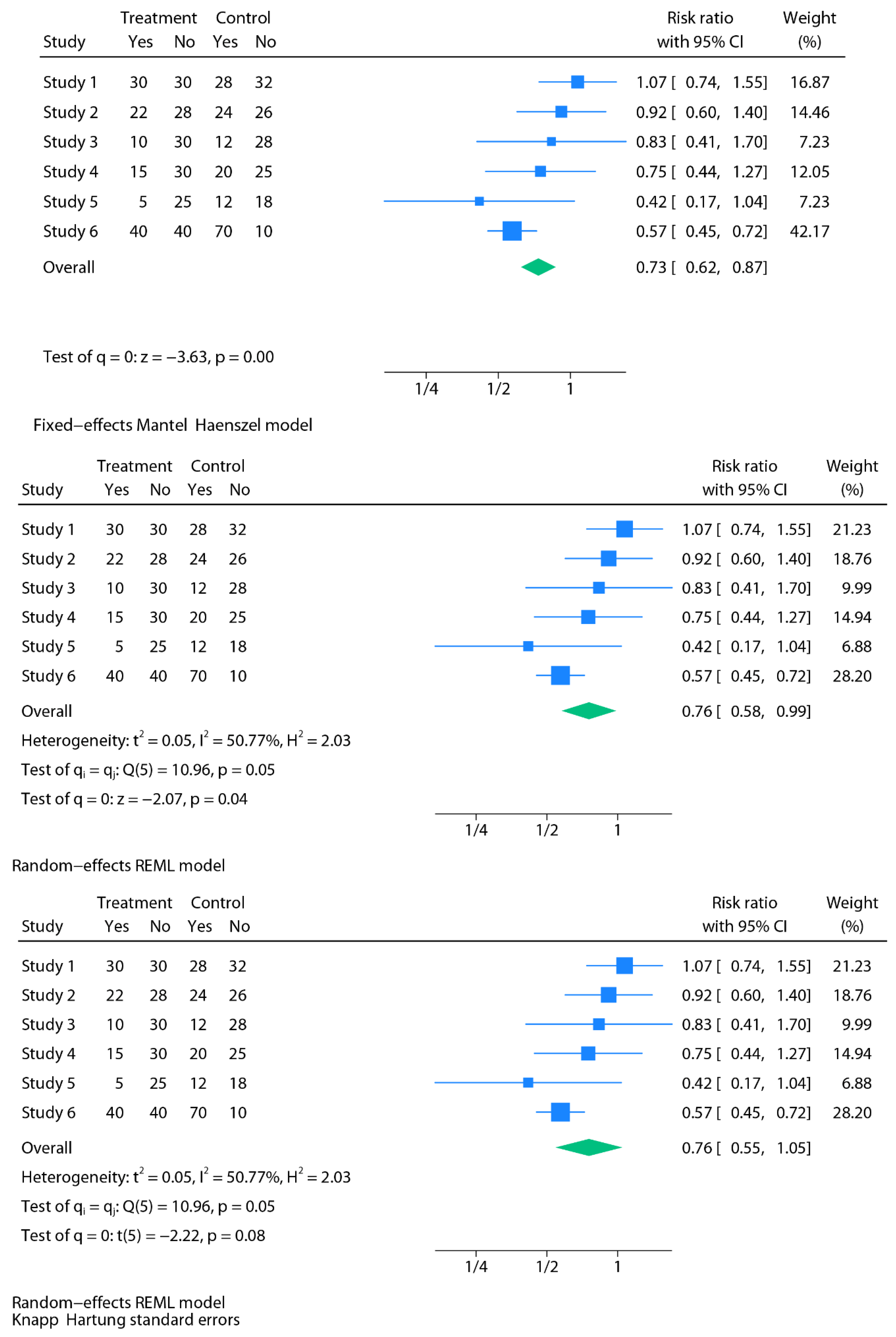

Table 1.
Illustrative and simplified clinical scenarios contrasting the assumptions of fixed-effect and random-effects models.
Table 1.
Illustrative and simplified clinical scenarios contrasting the assumptions of fixed-effect and random-effects models.
| Clinical Scenario | What does assuming fixed effects mean | What does assuming random effects mean |
|---|---|---|
| In non-operative management of uncomplicated appendicitis (antibiotics alone), is the success rate the same across all hospitals? | Assumes that non-operative antibiotic management yields the same success rate everywhere, with any between-hospital differences attributed only to chance. | Recognizes that true success rates differ—e.g., ~90% in some centers and ~70% in others—owing to patient selection, imaging protocols, antibiotic regimens, criteria for failure/crossover, and local care pathways. |
| Do ACE inhibitors lower blood pressure by the same amount in every patient? | Assumes that all patients experience an identical reduction (e.g., 10 mmHg), with observed deviations dismissed as random noise. | Recognizes that true responses vary according to patient- and context-specific factors—such as race (e.g., Black patients often respond differently to ACE inhibitors), comorbidities, baseline blood pressure, and treatment adherence. |
| Does screening colonoscopy reduce colorectal cancer mortality equally in all health systems? | Assumes that screening colonoscopy provides the same mortality reduction regardless of context. | Recognizes that the benefit of screening colonoscopy varies according to program- and practice-level factors. For example, mortality reduction is greater in robust, high-coverage programs and smaller in under-resourced systems; likewise, differences in endoscopist quality—such as adenoma detection rates—also influence the magnitude of effect. |
| Does prone positioning reduce mortality in ARDS patients to the same extent across ICUs? | Assumes a uniform mortality reduction across all settings (e.g., 15%). | Recognizes that the benefit varies according to multiple factors. For example, outcomes may be better in experienced centers with established protocols, adequate nurse-to-patient ratios, and optimal ventilatory management, compared to smaller units with less prepared staff. These are illustrative factors that influence the true effect, rather than random noise. |
| Do COVID-19 vaccines protect against infection? | Assumes identical vaccine effectiveness across all groups, regardless of age, comorbidity, or circulating variants. | Recognizes that effectiveness genuinely varies, with higher protection in some groups and lower in others, the pooled estimate reflecting an average across these conditions. |
| Does a smoking cessation intervention increase quit rates equally across settings? | Assumes that this intervention produces the same improvement in quit rates everywhere, with any observed variation across studies explained only by chance. | Recognizes that effectiveness depends on contextual and patient-level factors—for example, behavioral support intensity, pharmacotherapy access, or patient characteristics—so that observed differences reflect genuine variability rather than random noise. |
ACE = angiotensin-converting enzyme; ARDS = acute respiratory distress syndrome; ICU = intensive care unit.
Table 2.
Choosing between fixed and random-effects: a clinician’s guide.
| Criterion | Fixed-effect (common-effect) model | Random-effects model |
|---|---|---|
| Underlying assumption | Assumes a single true effect applies to all studies; observed differences are due only to chance. | Assumes true effects vary across studies; the pooled estimate represents the average of a distribution. |
| Clinical diversity | Suitable only when studies are essentially identical in population, intervention, and setting. | Preferred when studies differ in patients, protocols, or healthcare contexts. |
| Number of studies | Appears stable with very few studies, but precision is often misleading | Safer with few; use HKSJ to better reflect uncertainty. HKSJ may be over-conservative with very few studies; consider modified/truncated HKSJ (mHK) |
| Statistical heterogeneity | Ignores between-study variability; heterogeneity is treated as sampling error. | Explicitly incorporates between-study variability into the analysis. |
| Precision vs realism | Produces narrower confidence intervals that may overstate certainty. | Produces wider intervals that better reflect real-world uncertainty. |
| Generalizability | Limited; results apply only to the specific studies included. | Broader; results are more applicable across diverse contexts. |
| Role in practice | Occasionally useful for sensitivity analyses or narrowly defined questions. | Default choice in most clinical meta-analyses. |
Table 3.
Explicit recommendations from the Cochrane Handbook for Systematic Reviews.
| Criterion | Fixed-effect (common-effect) model | Random-effects model |
|---|---|---|
| Underlying assumption | Assumes a single true effect applies to all studies; observed differences are due only to chance. | Assumes true effects vary across studies; the pooled estimate represents the average of a distribution. |
| Clinical diversity | Suitable only when studies are essentially identical in population, intervention, and setting. | Preferred when studies differ in patients, protocols, or healthcare contexts. |
| Number of studies | Appears stable with very few studies, but precision is often misleading | Safer with few; use HKSJ to better reflect uncertainty. HKSJ may be over-conservative with very few studies; consider modified/truncated HKSJ (mHK) |
| Statistical heterogeneity | Ignores between-study variability; heterogeneity is treated as sampling error. | Explicitly incorporates between-study variability into the analysis. |
| Precision vs realism | Produces narrower confidence intervals that may overstate certainty. | Produces wider intervals that better reflect real-world uncertainty. |
| Generalizability | Limited; results apply only to the specific studies included. | Broader; results are more applicable across diverse contexts. |
| Role in practice | Occasionally useful for sensitivity analyses or narrowly defined questions. | Default choice in most clinical meta-analyses. |
ACE = angiotensin-converting enzyme; ARDS = acute respiratory distress syndrome; ICU = intensive care unit.
Table 4.
Reporting essentials for a meta-analysis.
| Section | What should be reported | Why it matters |
|---|---|---|
| Methods |
|
Transparency; reproducibility; avoids selective reporting. |
| Results |
|
Ensures clarity; communicates both precision (CI) and expected variability across contexts (PI); readers understand robustness of findings. |
τ² = between-study variance; I² = inconsistency index; Q = Cochran’s Q test; CI = confidence interval; PI = prediction interval; DL = DerSimonian–Laird; REML = restricted maximum likelihood; HKSJ = Hartung–Knapp–Sidik–Jonkman; CMA = Comprehensive Meta-Analysis; RevMan = Review Manager.
Table 5.
Summary of how conclusions shifted in five real-world case studies when re-analysed under random-effects models.
Table 5.
Summary of how conclusions shifted in five real-world case studies when re-analysed under random-effects models.
| Case study | Clinical question | Original model & result | Re-analysed model & result | Key lesson |
|---|---|---|---|---|
| 1. Urination stimulation in infants | Non-invasive stimulation to collect urine samples | FE Mantel–Haenszel: OR 3.88 (95% CI 2.28–6.60), p<0.01; I²=72% → strongly positive | RE REML: OR 3.44 (1.20–9.88), p=0.02; HKSJ: OR 3.44 (0.34–34.91), p=0.15 → wide, inconclusive | FE overstates precision; RE + HKSJ highlight the underlying uncertainty. With very few studies, confidence intervals become challenging to interpret—either too narrow under FE or excessively wide under HKSJ—underscoring the inherent difficulty of sparse-data scenarios |
| 2. Esophageal atresia repair | Musculoskeletal sequelae after thoracoscopic vs open repair | FE Mantel–Haenszel: RR 0.35 (0.14–0.84), p=0.02 → significant reduction | RE REML: RR 0.35 (0.09–1.36), p=0.13; HKSJ: RR 0.35 (0.05–2.36), p=0.18 → loss of significance | Certainty collapses when heterogeneity is acknowledged; RE prevents false confidence |
| 3. Psychological Bulletin re-analysis | 68 psychology meta-analyses re-examined | FE gave narrow, often “significant” CIs; apparent robustness | RE widened CIs, significance often disappeared; FE defensible in ~3% only | Large-scale evidence that FE systematically exaggerates certainty |
| 4. Rosiglitazone & CV risk | Myocardial infarction & cardiac death with rosiglitazone | FE: MI RR 1.43 (1.03–1.98), p=0.03 (↑ risk); cardiac death RR 1.64 (0.98–2.74), p=0.06 (NS) | RE (rare-event): MI RR 1.51 (0.91–2.48), p=0.11 (NS); cardiac death RR 2.37 (1.38–4.07), p=0.0017 (↑ risk) | FE masked real risk signal; RE exposed to clinically important harm |
| 5. Magnesium in acute MI | IV Mg²⁺ for AMI | FE: OR 1.02 (0.96–1.08) → null; extreme heterogeneity (p<0.0001) | RE: OR 0.61 (0.43–0.87), p=0.006 → protective | FE obscured mechanistic truth; RE aligned with biological plausibility (timing of administration) |
FE = fixed-effect; RE = random-effects; REML = restricted maximum likelihood; HKSJ = Hartung–Knapp–Sidik–Jonkman; OR = odds ratio; RR = risk ratio; MI = myocardial infarction; AMI = acute myocardial infarction.
Table 6.
Takeaway messages.
|
Disclaimer/Publisher’s Note: The statements, opinions and data contained in all publications are solely those of the individual author(s) and contributor(s) and not of MDPI and/or the editor(s). MDPI and/or the editor(s) disclaim responsibility for any injury to people or property resulting from any ideas, methods, instructions or products referred to in the content. |
© 2025 by the authors. Licensee MDPI, Basel, Switzerland. This article is an open access article distributed under the terms and conditions of the Creative Commons Attribution (CC BY) license (http://creativecommons.org/licenses/by/4.0/).
Copyright: This open access article is published under a Creative Commons CC BY 4.0 license, which permit the free download, distribution, and reuse, provided that the author and preprint are cited in any reuse.


