Submitted:
28 August 2025
Posted:
01 September 2025
You are already at the latest version
Abstract
Given that most microbes experience spatially structured environments, examining how such environments affect microbial growth and functions is paramount. Previous studies have shown that a spatially structured environment can impact microbial growth and interactions, and that microbial growth can create or magnify spatial structure. Here, we review some of these instances of past studies to develop a consistent framework that highlights the interplay between microbial interactions, spatial structure of the environment, and spatial organization of microbes. We discuss how mathematical models can reveal the contribution of the spatial structure to community assembly and coexistence. Lastly, we offer an outlook of important steps for the progress of this field.
Keywords:
microbial communities
; coexistence
; spatial structure
; spatial organization
; microbial interactions
1. Introduction
1.1. What is Spatial Structure?
In the context of microbial ecology and evolution, a spatially structured environment is one in which individual microbes experience different local conditions [1]. This environment can include abiotic factors, such as temperature or physical barriers, or biotic factors, such as the physical presence of other microbes or a gradient of their metabolic byproducts. A spatially structured environment is defined in contrast with a uniform (also called homogeneous or well-mixed) environment in which all individual microbes experience exactly (or almost exactly) the same conditions in their environment. As one would expect, most microbes live in spatially structured environments. Individual microbes may experience different environments because of several reasons. The environment may not be uniform, and individuals may experience different levels of temperature, pH, nutrients, or oxygen availability, for example. Every cell within a biofilm may experience different local conditions, simply due to having different numbers and types of neighboring cells around it. Some microbes may be spatially associated with other microbes, for example because of physical aggregation. Even when there may not be exchange of molecules between two microbes, the competition for locally available nutrients means that one microbe affects other microbes in its vicinity. In this sense, living in a spatially structured environment is the norm rather than the exception.
1.2. The Level and Degree of Spatial Structure
The impact of spatial structure can be examined at different levels [2], from cell-level, i.e. the influence between individual cells, to population-level, i.e. the net effect between populations of cells. For the majority of our following discussions, we choose to focus on the population-level scale. With this choice, the impact of a spatial environment is still represented but is simplified into net effects on populations, allowing direct comparison with well-mixed counterparts. Each population designates a specific ‘type’ of cell which, depending on the context of interest, may refer to a community, a phylogenetic group (such as a phylum, a genus, a species, or a strain), or even phenotypically different groups within the same genotype [3]. For each population, we define its spatial distribution as how that population is spread across space. The spatial distribution of each population is often the product of many different factors, from environmental influences and extracellular matrix production to interpopulation interaction and cell motility [4]. Motility, in particular, can have a profound impact on the spatial distribution of populations, especially when considering processes such as chemotaxis, collective response, or quorum sensing [5,6,7].
The presence or absence of spatial structure conceptually is defined based on whether individuals within a population experience the same environment [1]. Considering that the mere presence of other individuals changes the environment experienced by each individual (e.g. in a colony), it is clear that the absence of spatial structure is only an abstract theoretical possibility. However, the degree of spatial structure matters. For example, whether individuals from one population are clustered with their own type or are distributed among a partner population can influence the access to resources and interpopulation interactions.
Several metrics have been defined in ecological studies to quantify the degree of spatial organization of organisms, resources, and environmental factors. These metrics can be broadly divided into three groups: (1) Spatial autocorrelation metrics [8], such as Moran’s I or Geary’s C, which quantify the degree of similarity or dissimilarity at nearby spatial locations to represent the degree of clustering or dispersion. (2) Point pattern analysis metrics [9], such as nearest neighbor distance analysis or Ripley’s K function, to assess whether the distribution of individuals in the domain of interest is random or structured. (3) Landscape ecology metrics [10], such as metrics for patch size, shape, distribution, and connectivity, which measure how patches are spread across a landscape. In practice, a modified version of such metrics is often used, tailored to the biological phenomenon of interest. For example, Maire et al. and Dang et al. introduced a spatial correlation function weighted by the communication strength between every pair of cells to represent a spatial index I [11,12]. This single number captured the degree of order in the spatial structure, as related to the spatial self-organization of cells communicating via one or more diffusible ligands.
1.3. The Scale of Spatial Structure
Related to the idea of the degree of spatial structure is the scale of biological processes in a community. Temporal and spatial scales are often of particular interest—the relevant time over which the biological processes of interest occur and the relevant spatial reach of these processes. The relevant scales can be substantially impacted by the underlying physical processes that are in effect, such as the spread of nutrients in an environment by diffusion versus by flux or transport. Depending on the underlying processes, the temporal and spatial scales can also be linked. For example, two processes commonly governing metabolite-mediated interactions are diffusion and transport. If an interaction is driven by a diffusion process, the temporal scale and spatial scale are related as . In contrast, with flux or transport processes, , where is the transport speed in the environment. It is important to note that such relationships can have profound consequences. For instance, if a metabolite spreads in space by diffusion, it is unlikely for it to reach long distances within relevant time scales. Assuming a relatively large diffusion coefficient of , diffusion takes a metabolite a distance of 100 µm, 1 mm, and 10 mm in approximately in 15 seconds, 25 minutes, and 42 hours, respectively. In contrast, the time required for transport linearly scales with distance.
Previous reports have also examined the consequences of spatial scale. For instance, Hart et al. examined whether a certain spatial scale is required to maintain species diversity [13]. They introduced the coexistence-area relationship as a practical measure to represent how coexistence can be driven by the spatial scale of the environment. As another example, Song et al. have shown that when interactions had the same spatial scale as the spatial distributions, increased motility negatively impacted diversity in an engineered model of interpopulation exploitation [14]. As another example, Luo et al. showed that a structured environment may also suppress cooperation by allowing cheaters to more effectively exploit the cooperators [15].
1.4. Functional Consequences of Spatial Structure
From a practical point of view, the motivation behind examining spatial structure is to understand its functional consequences. Some impacts of spatial structure on microbial communities and their functions are intuitive. It is easy to imagine how restricting the access of interaction partners to each other affects the outcomes; notably, as Gause showed, prey-predator coexistence may depend on the ability of prey to avoid the predator in a spatial refuge [16]. Later it was shown that a simple spatial structure of two connected patches might be enough to allow the prey to stably persist in a predator-prey system [17]. Population distributions can also be functionally consequential. For example, wastewater microbial granules have layers of different microbial populations and successively break down complex compounds; such granules will not work as effectively if the order of species is reversed [18]. Spatial structure can also change the intensity of competition. This has been shown in plant systems, when slow growers could persist in a spatial environment in direct competition with fast growers, if the slow growers were better at colonizing new territory compared to fast growers [19]. In a bacterial system, Gude et al. showed that in a patchy spatial environment, a trade-off between motility and competitive advantage can allow bacterial populations to coexist [20]. Several additional examples that highlight the impact of spatial structure are reviewed nicely in [21].
Spatial structure has been found to influence species interactions in several empirical studies. We highlight a few past examples, noting that these examples are chosen not to comprehensively represent the prior work but to bring up some of the underlying mechanisms and concepts. Kim et al. used microfluidic chambers connected via channels to assess how spatial separation between populations can affect coexistence. They observed that when the spacing was too short, competition dominated and disrupted coexistence, and when the spacing was too long, facilitative interactions became too weak to sustain coexistence; coexistence was achieved at intermediate spatial spacing between these extremes [22]. Harcombe et al. examined the spatial arrangement of different populations. They observed that metabolic interactions between two partner populations may be intercepted by other populations that are spatially situated between the two partners—they referred to this phenomenon as the metabolic ‘eclipse’ effect [23]. In our own prior work, we have shown that in a system of cooperators and cheaters, spatial self-organization driven by species interactions can favor cooperation and disfavor cheating [24]. Datta et al. explored how spatial structure at the expanding range of a community reshaped distance between different phenotypes and thereby influenced their competition and the trajectory of evolution [25]. In these studies, the role of spatial distance between interacting populations in modulating their interactions is noteworthy.
In the rest of this paper, we take the simplified view of examining the role of spatial structure in creating or modifying the feedback [26] between the environmental constraints, the survival and growth of populations in those environments, and the resulting spatial distributions of the populations (Figure 1A). Taking one additional step towards a more mechanistic representation, we examine population interactions in the spatial context and how they might act as an intermediate in the interplay between the environment, growth, and patterns (Figure 1B). The interactions, for example by competition for resources, cross-feeding, or release of inhibitory compounds, take place at a cellular level, but the ‘population interactions’ terminology refers to the net effect of interactions on a population across the community and depends on the spatial distribution of the interacting populations.
2. The Drivers of Spatial Structure in Microbial Communities
Spatial structure can be generated by abiotic or biotic processes. Abiotic structure might be the result of existing heterogeneity in the environment, which leads to individuals experiencing different environments, for example across a gradient of oxygen [27], nutrients [28], or light [29]. In contrast, biotic spatial structure can be caused either by the physical presence of other organisms in the environment, by the heterogeneity in the environment caused by the activity of other populations, or even by population heterogeneity arising from noisy gene expression within an isogenic population. Competition for space in territorial populations [30]—when populations occupy spatial locations and exclude others from those locations—can be considered an example of the former, and the heterogeneous distribution of a beneficial mediator in commensalisms between two species [31,32] would be an example of the latter. These drivers of spatial structure rarely work in isolation. The spatial structure of a microbial community is often the result of several factors, both biotic and abiotic, dynamically changing and modulating each other. This intricate interplay makes spatial distribution patterns complex and context-dependent. A well-known manifestation of this interplay is the emergence of Turing patterns from a combination of short-range facilitation and long-range inhibition interactions [33,34].
From a different perspective, how the structure is generated can be categorized into two different types: guided versus self-organized (also called non-autonomous versus autonomous [35]). Guided spatial structure refers to situations in which the spatial distribution of populations is driven by external factors. These external factors could be imposed by the physical and/or chemical constraints of the environment, including abiotic environmental heterogeneity, or by signals and/or cues generated by populations within the community. As an example, an external oxygen gradient could restrict the presence of some anaerobic oral bacteria to regions below the gum line in the mouth [36]. Self-organized spatial structure can be either internally coordinated or interaction driven. Internally coordinated spatial structure refers to situations in which the spatial distribution of populations is driven by an evolutionary adapted genetic program. Conceptually, this is akin to coordinated patterns developing in multicellular organisms [37]. Examples of internally coordinated self-organized spatial patterns include the phenotypic differentiation in B. subtilis biofilms [3,38], metabolic differentiation in S. cerevisiae colonies [39], or cell differentiation in stalk-like structures of S. cerevisiae [40]. Interaction driven self-organized spatial structure refers to situations in which spatial patterns emerge from interactions among populations [41]. Examples of Interaction driven self-organized spatial patterns include the spatial intermixing of mutualists [31], spatial isolation of cheaters [24], spatial isolation of antibiotic-sensitive members from antibiotic-producers [42], or engineered patterns in synthetic populations [43]. A defining feature of self-organized spatial structure is that it can be explained by intra- and inter-population interactions among the constituents of the community, without necessarily involving evolutionarily selected programs for patterning. We acknowledge that the distinction between different types of guided versus self-organized patterns may not be clear in communities in which the interactions and molecular mechanisms are less known.
In what follows, we will briefly survey some examples of driving forces that can generate spatial structure and influence interactions in microbial communities.
2.1. Abiotic Spatial Heterogeneity
The heterogeneous environment can take many forms. There are instances where heterogeneity that microbes experience is intrinsic to the abiotic environment. For example, the porous soil structure generates a patchy environment [44] and affects the transport of water through the soil and subsequently impacts microbial interactions and functions (Figure 2A). On the surface of skin, glands and hair follicles offer heterogeneous shelter to bacterial populations (Figure 2B) [45]. Similarly, in bacterial colonization of wounds, different zones in this heterogeneous environment allow different bacteria to persist (Figure 2C). Although in the last two examples the host is a living organism, from the perspective of microbes and for a limited timescale, it can be viewed as static, similar to an abiotic environment.
2.2. Biotic Spatial Heterogeneity via Population Viscosity
A major driver of biotic spatial structure is population viscosity—a phenomenon in which progenies remain physically close to their parents, being unable or slow to disperse away (Figure 2D). Often such population viscosity leads to increased intrapopulation interactions over interpopulation interactions [46]. During range expansion of mixed populations, for example, this competition becomes an important factor in how different populations compete as they take over new territory [32,47,48].
2.3. Biotic Spatial Heterogeneity via Niche Construction and Ecosystem Engineering
In many cases, the microbial populations themselves are a major contributor to the spatial structure of the environment. Conceptually, this can be viewed as niche construction, changing the environment experienced by those populations as well as other populations encountering that habitat (Figure 2E). For example, altruistic cell death and toxin release by a competitively disadvantaged strain can create a zone in which that strain can survive and prosper in a spatial environment [49]. A conceptually similar phenomenon is species creating spatial gradients of environmental resources and properties. For example, in a multispecies community that degrades cellulose, obligate aerobes in a static liquid culture can create a low-oxygen zone for oxygen-sensitive cellulolytic members to survive and contribute to the community function [50,51]. Aerobic nitrifying bacteria and anaerobic ammonium oxidizing bacteria work together and form micro-granule with a layered structure [52]. In oral microbiota, early-colonizers create a spatial niche in which attachment of others to these early-colonizers is a critical component of community development [53]. Primary producer cyanobacteria can create anoxic zones in aggregates that support stable persistence of heterotrophs [54]. Even more directly, the extracellular matrix generated by microbial species in biofilms can create the spatial structure within which other cells are distributed and organized [55,56].
Overall, the spatial structure of a microbial community can have different sources. It can originate from external biotic or abiotic sources, from the activities of each population, from the presence or activities of other populations within the community, or a combination of these sources. Recognizing which sources contribute to the spatial structure of a community can be important for better understanding how the spatial structure of the community establishes, persists, or progresses.
3. How Interactions Are Affected by the Spatial Context
The spatial context can determine what populations within the community interact with each other, how often they can interact, and what outcomes emerge from those interactions. In a simplified view, access to the partner is the primary factor that directly modulates interactions. Spatial self-organization, driven by microbe-environment and microbe-microbe interactions can also influence population distributions and subsequently affect interactions.
3.1. Access to a Partner
One of the primary ways that spatial structure affects population structure is through affecting interaction opportunities among cells. Guided spatial structure can influence the chance of interactions between species. As an example, environmental compartments in Gause’s study of prey-predator dynamics allow the prey to avoid the predator [16]. An intuitive example of species-driven structure affecting access to partners happens with population viscosity: accumulation of progeny around dividing cells increases the likelihood of encounters and interactions within the same population and decreases the likelihood of interactions with other populations [57]. The eclipse effect mentioned earlier and shown by Harcombe et al. underscores another facet of access, when a population intercepts the interaction mediators and blocks or weakens interactions between other populations [23].
A key determinant of access to the partner is the spatial distance between cells of each population from other cells of their own population or other populations. In their seminal work, Kim et al. used controlled experiments in connected microfluidic chambers to show that the strength of interactions could be modulated by changing the distance between populations [22]. A clear manifestation of the role of distance is in the interspecies syntrophic hydrogen transfer in syntrophic methanogenic consortia [58]. The dependency of interactions on the spatial distance between populations can take different forms. Romdhane and colleagues conceptually categorize the dependency into three possibilities: independent, linearly decreasing, and threshold-based [59]. For interactions that rely on metabolite exchange or influence, the linear dependence likely indicates that they can be associated with transport processes. In contrast, threshold-based interactions are likely associated with diffusion processes, where long-range interactions at relevant timescales are not expected (see Section 1.3).
3.2. Microbial Interactions Can Be Modulated by Spatial Self-Organization
Self-organized spatial structure—ordered spatial structure emerging from interactions within the community—can also change intra- and inter-population interactions. These changes often follow certain trends based on the intrinsic feedback between population growth, spatial patterns, and interaction-driven dynamics. When driven by interpopulation interactions, spatial self-organization often favors facilitation and disfavors inhibition [60]. This trend is intuitive, as growth of each population in space will be favored in regions that are closer to facilitatory partners and away from inhibitory ones (Figure 3). The emergence of patterns such as intermixing of mutualists, layered pattern of commensal, and segregation of competitors, is the result of this trend [24,61].
4. How Coexistence Is Affected by the Spatial Context
4.1. Niche Partitioning Enabled by Spatial Heterogeneity
Spatial context can be an important factor to permit and maintain coexistence. A primary concept through which coexistence is supported in a spatial structure is through niche partitioning [62]. Niche partitioning is defined as the process by which different populations access different resources or niches within a community, often leading to reduced competition and more coexistence. As an example, spatial structure can support the coexistence of antagonistic competitors in a patchy environment, with each patch dominated by one or the other competitor who has gained majority within that patch [63]. The weaker competitors can persist by occupying patches or microhabitats where they escape competition by other competitors. Strong spatial heterogeneity can preserve diversity by diminishing the chance of fixation for advantageous mutations; however, this barrier can be overcome if the mutant has improved migration capability [64].
Niche partitioning can also be enabled by different ecological strategies of coexisting populations. For example, coexistence between marine bacterioplankton populations of V. cyclitrophicus in a nutrient patchy environment may be supported by different utilization/dispersal strategies: one population specializing in accessing localized resources within each patch and the other population specializing in dispersing and discovering new patches [65].
4.2. Successional Niche Occupation
Niche partitioning can also happen through temporal succession. For example, spatial dynamics can contribute to coexistence by allowing successive colonization of patches by different populations, a process called successional niche occupation. Conceptually, this can be considered to be another manifestation of niche partitioning—in time rather than space—enabled by dispersal among interconnected patches. Hassell et al., for example, showed that dispersal in a patchy environment can support coexistence of competitors, even if patches are identical. They interpreted this phenomenon as self-organized spatial dynamics [66]. Similarly, spatial heterogeneity has been shown to allow the stabilization of predator–prey interactions by allowing spatial dynamics across interconnected patches [67]. Successional niche occupation can also involve the generation of new spatial niches by other populations. For example, early colonizers in oral microbiota generate a new niche by creating opportunities for cell adhesion for the successors [68,69].
4.3. Loss of Coexistence Due to Spatial Isolation
A pronounced spatial structure may not always support more coexistence. For example, slower diffusion of interaction mediators in the environment—making the effect of the spatial structure stronger—also weakens interpopulation facilitation and may lead to less coexistence overall [70,71]. Snyder and Chesson examined the interplay between dispersal, competition, and environmental heterogeneity and found that depending on the scales of different processes, the overall effect could either promote or suppress coexistence [72].
4.4. Populations-Driven Spatial Self-Organization
In addition to spatial heterogeneity of the environment itself, spatial self-organization emerging from species activities can also generate or modify niches and influence coexistence. For instance, in a community of antibiotic-producer, antibiotic-sensitive, and antibiotic-resistant bacteria, spatial patterns emerged, driven by interactions through antibiotics, that allowed coexistence [42].
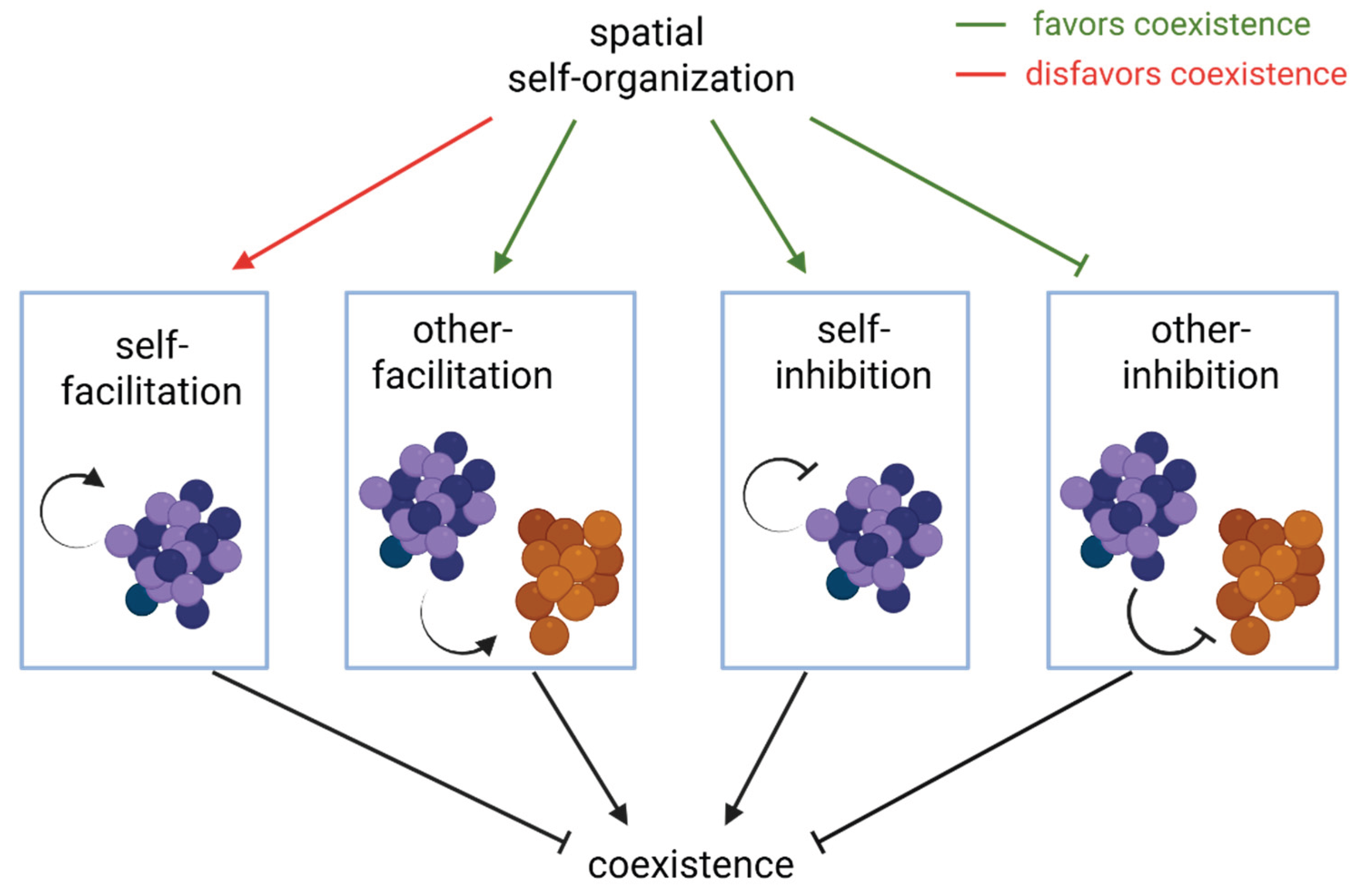
In a simplified view, three prominent trends can contribute to higher coexistence and diversity in spatial communities (Figure 4): (1) magnifying intrapopulation competition for resources over interpopulation competition [73], (2) reinforcing inter-population facilitation by spatial intermixing [31], and (3) suppressing inter-population inhibitory effects by spatial segregation of antagonistic populations [74]. Coexistence can also be driven by spatial patterns arising from interactions between the populations and the environment. For example, in biofilms of Klebsiella pneumoniae and Pseudomonas aeruginosa, different attachment and detachment rates can balance the competitive advantage and allow coexistence [75].
Emergent spatial patterns can also act against coexistence. For example, in a community of cooperators and cheaters, self-organization and intermixing of cooperators can spatially isolate cheaters and drive them to extinction [24]. Spatial structure can also amplify self-facilitation—a population converting resources to a beneficial factor for its own—which can be useful for maintaining competitively disadvantaged populations but can also act as a destabilizing force by providing positive feedback [70].
5. The Impact of Spatial Structure Through the Lens of Mathematical Models
Mathematical modeling offers a complementary source of insights, enabling more control to set up desired assumptions and arrangements and more transparency to facilitate the interpretation of the outcomes. These in turn allow more mechanistic investigations into how and by how much the spatial context contributes to community outcomes. Below we briefly summarize a few conceptual models, each capable of capturing the relevant biological processes and the impact of spatial structure within a range of scales and assumptions. Even though we present these models as separate entities, a mathematical model can be a combination of these models, capturing each relevant process using a corresponding model at an appropriate scale and level of abstraction.
There are different levels of simplification to capture the main aspects of spatial structure, and a choice can be made on how to represent the system. As Durret and Levin put it [1], “[this choice] goes far beyond the mathematical convenience to the heart of understanding the mechanism,” especially to unravel what mechanisms are important for explaining spatial phenomena of interest.
At one extreme, the simplest representation is a mean-field model which captures how on average the spatial structure affects the populations experiencing that environment. When a global average adequately represents the net effect on a population in a spatial context, the mean-field model offers significant simplification. However, the expectation is that when there is significant heterogeneity in the environment, significant structure in population distributions, or short-range interactions are dominant, a mean-field model may not capture the details of spatial distribution.
Patch models, predominantly used in ecological studies, refer to representations in which the environment consists of well-mixed patches connected by a network of links between patches. With limited dispersal, the environment will become structured as individuals within the same patch interact more strongly with each other compared to individuals residing in different patches [76].
Recognizing diffusion as a primary process for population dispersal and chemical spread in the environment, reaction-diffusion models are often utilized [31,70]. The essence of these models considers agents that can move or spread in the environment (e.g. via random walk [77]) and interact with other agents through defined reactions. These models can also capture how chemical compounds, such as nutrients, toxins, and metabolic byproducts, mediate microbial interactions [78,79].
A more explicit approach is to explicitly simulate individual cells/units within a population along with the relevant processes for their interactions in an agent-based model [11,12,80,81,82]. Keeping track of individuals, their unique environment, and possibly even their unique properties (or behaviors) allow a detailed representation of the microbes in a spatial context. Such a detailed presentation of patterns and dynamics can reveal complex dynamics emerging from individual-level rules. The downside is that such models require an understanding of the detailed mechanistic rules that apply to individuals and are often computationally intensive.
6. Outlook: What Is Next?
6.1. Measuring Spatial Patterns in Nature
Although the impact of spatial structure in microbial communities has been studied in many examples, there is still room to explore the mechanisms involved in the emergence and maintenance of community patterns. A necessary step for proper interpretation of the role of space is developing the tools and techniques to observe the spatial details of communities. Recent advances in multimodal and multiplexed imaging is one of the significant steps forward, allowing detailed characterization of the spatial positioning of cells [83,84] and the spatial profile of the chemical environment [85,86]. Advances in sequencing have also complemented this progress by offering the capability to monitor the spatial distribution of microbial populations [87], proteins, and metabolites.
6.2. Controlling Spatial Structure and Pattern
A major shift in recent years has been in making laboratory-based studies more realistic. An important aspect of such efforts involves better representation of the intrinsic spatial structure of the corresponding biological system. A variety of examples, from artificial soil to organ-on-a-chip devices underscore the recent advances and highlight the impact of the spatial context [88,89,90].
The technical difficulties of controlling the spatial arrangement of cells poses limitations on how detailed studies can be designed for spatial studies. Advances in microfluidics [22,91] and bioprinting [92,93] have already taken steps to address this shortcoming. Recent technological improvements in these areas have made these strategies more accessible and broadly applicable.
6.3. Designing Community Functions in a Spatial Context
An important step toward implementing synthetic communities with desired functions is to utilize the spatial context for stability or enhanced functionality. For example, Kim et al. implemented pre-structured synthetic communities to control community processes and achieve efficient degradation of organic pollutants in the presence of inhibitory heavy metals [91]. Beyond pre-structuring, programmed pattern formation can be viewed as an additional design opportunity [35]. Maintaining microbial populations is thought to be a main challenge in consolidating bioprocessing [94], and programmed pattern formation can offer a solution for maintaining important community functions.
6.4. Accounting for Evolution in a Spatial Context
A better understanding of coexistence in a spatially structured environment cannot be achieved without considering evolutionary processes. There are several ways that spatial structure can impact the trajectory of evolution and coevolution. Spatial structure can create the niche for the rise of certain mutations and genotypes [55]. For example, Chao et al. showed that a toxin-producer genotype was disfavored in well-mixed environments and could arise only when the spatial structure localized the competitive benefits to the toxin-producing genotype [49]. In phage-bacteria dynamics, Kerr et al. showed that unrestricted dispersal selected for more aggressive phage and loss of productivity, whereas restricted migration favored prudent phage and averted the tragedy of the commons [95]. Spatial structure can also reshape interpopulation interactions. For example, Hansen et al. demonstrated that the interaction between Pseudomonas and Acinetobacter in a community transitioned from commensalism to exploitation only in a spatially structured environment [96]. The evolution of spatially relevant traits is another aspect enabled by the spatial context. For instance, Parvinen et al. have shown that under different circumstances, such as the presence or absence of temporal heterogeneity, spatial heterogeneity can have opposing effects on the evolution of dispersal [97]. Lastly, as an example of coevolution, Hochberg and van Baalen have examined the evolution of a prey-predator system in a patchy system and found that within-population diversity was highest in habitats at intermediate levels of productivity [98]. Although not comprehensive, the above examples serve as snapshots of some of the ways through which evolutionary processes both impact the spatial structure and are impacted by it.
6.5. Concluding Remarks
Studying microbial communities is motivated by the need to understand the mechanisms involved in microbiota functions and ecosystem processes. Given that the spatial context is often an intrinsic feature of microbial communities, here we have highlighted what processes the spatial structure stems from, how the spatial context affects interactions among different populations within a community, and how the spatial structure influences community properties, including properties as fundamental as coexistence of community members. In our treatment of the spatial structure and its role, we have used conceptual simplifications to find common threads among diverse and often complex microbial systems. Rather than delving into the complexities of each system, we simplified the representation by focusing on general concepts such as the localization of populations, average distance among interacting populations, and interaction-driven self-organization. These simplifications, in our opinion, provide intuitive—even if not fully accurate—guidelines about the essence, emergence, and progression of spatial structure for microbial communities. The next milestone, in our opinion, is to take this insight and apply it to control the structure and function of microbial communities. Towards this goal, recent progress in quantifying the extent and impact of spatial structure, in controlling the distribution of microbial populations within a community, and in incorporating microbial ecology and evolution in designing spatial communities are important and promising steps.
Acknowledgments
This work was supported by a grant from the National Science Foundation (NSF-MCB Grant No. 2430384). ER and YC were partially supported by Undergraduate Research Fellowships from Boston College. HY was supported by a grant from the National Institutes of Health (NIH-NIGMS R35 Grant, GM147508).
Competing Interest
The authors declare that they have no known competing interests.
References
- Durrett R, Levin S (1994) The Importance of Being Discrete (and Spatial). Theor Popul Biol 46:363–394. [CrossRef]
- Borisy GG, Valm AM (2021) Spatial scale in analysis of the dental plaque microbiome. Periodontol 2000 86:97–112. [CrossRef]
- Vlamakis H, Aguilar C, Losick R, Kolter R (2008) Control of cell fate by the formation of an architecturally complex bacterial community. Genes Dev 22:945–953. [CrossRef]
- Booth SC, Rice SA (2020) Influence of interspecies interactions on the spatial organization of dual species bacterial communities. Biofilm 2:100035. [CrossRef]
- Mohanty S, Firtel RA (1999) Control of spatial patterning and cell-type proportioning in Dictyostelium. Semin Cell Dev Biol 10:597–607. [CrossRef]
- Ben-Jacob E, Cohen I, Levine H (2000) Cooperative self-organization of microorganisms. Adv Phys 49:395–554. [CrossRef]
- Parsek MR, Tolker-Nielsen T (2008) Pattern formation in Pseudomonas aeruginosa biofilms. Curr Opin Microbiol 11:560–566. [CrossRef]
- Getis A (2010) Spatial Autocorrelation. In: Handbook of Applied Spatial Analysis. Springer, Berlin, Heidelberg, Berlin, Heidelberg, pp 255–278. [CrossRef]
- Ben-Said M (2021) Spatial point-pattern analysis as a powerful tool in identifying pattern-process relationships in plant ecology: an updated review. Ecological Processes 2021 10:1 10:1–23. [CrossRef]
- Francis RA, Millington JDA, Perry GLW, Minor ES (2022) The Routledge Handbook of Landscape Ecology, 1st ed. Routledge.
- Dang Y, Grundel DAJ, Youk H (2020) Cellular Dialogues: Cell-Cell Communication through Diffusible Molecules Yields Dynamic Spatial Patterns. Cell Syst 10:82-98.e7. [CrossRef]
- Maire T, Youk H (2015) Molecular-Level Tuning of Cellular Autonomy Controls the Collective Behaviors of Cell Populations. Cell Syst 1:349–360. [CrossRef]
- Hart SP, Usinowicz J, Levine JM (2017) The spatial scales of species coexistence. Nature Ecology & Evolution 2017 1:8 1:1066–1073. [CrossRef]
- Song H, Payne S, Gray M, You L (2009) Spatiotemporal modulation of biodiversity in a synthetic chemical-mediated ecosystem. Nat Chem Biol 5:929–935. [CrossRef]
- Luo N, Lu J, Şimşek E, et al (2024) The collapse of cooperation during range expansion of Pseudomonas aeruginosa. Nat Microbiol 9:1220–1230. [CrossRef]
- Gause GF (1934) The Struggle for Existence. Baltimore: Williams & Wilkins.
- Jansen VAA (1995) Regulation of Predator-Prey Systems through Spatial Interactions: A Possible Solution to the Paradox of Enrichment. Oikos 74:384. [CrossRef]
- Satoh H, Miura Y, Tsushima I, Okabe S (2007) Layered structure of bacterial and archaeal communities and their in situ activities in anaerobic granules. Appl Environ Microbiol 73:7300–7307. [CrossRef]
- Tilman D (1994) Competition and Biodiversity in Spatially Structured Habitats. Ecology 75:2. [CrossRef]
- Gude S, Pinçe E, Taute KM, et al (2020) Bacterial coexistence driven by motility and spatial competition. Nature 2020 578:7796 578:588–592. [CrossRef]
- Tolker-Nielsen T, Molin S (2000) Spatial Organization of Microbial Biofilm Communities. Microb Ecol 40:75–84. [CrossRef]
- Kim HJ, Boedicker JQ, Choi JW, Ismagilov RF (2008) Defined spatial structure stabilizes a synthetic multispecies bacterial community. Proceedings of the National Academy of Sciences 105:18188–18193. [CrossRef]
- Harcombe WRR, Riehl WJJ, Dukovski I, et al (2014) Metabolic resource allocation in individual microbes determines ecosystem interactions and spatial dynamics. Cell Rep 7:1104–1115. [CrossRef]
- Momeni B, Waite AJ, Shou W (2013) Spatial self-organization favors heterotypic cooperation over cheating. Elife 2:e00960. [CrossRef]
- Datta MS, Korolev KS, Cvijovic I, et al (2013) Range expansion promotes cooperation in an experimental microbial metapopulation. Proceedings of the National Academy of Sciences 110:7354–7359. [CrossRef]
- Henderson A, Del Panta A, Schubert OT, et al (2025) Disentangling the feedback loops driving spatial patterning in microbial communities. npj Biofilms and Microbiomes 2025 11:1 11:1–14. [CrossRef]
- Ludemann H, Arth I, Liesack W (2000) Spatial Changes in the Bacterial Community Structure along a Vertical Oxygen Gradient in Flooded Paddy Soil Cores. Appl Environ Microbiol 66:754–762. [CrossRef]
- Codeço CT, Grover JP (2001) Competition along a spatial gradient of resource supply: a microbial experimental model. Am Nat 157:300–315. [CrossRef]
- Martinez JN, Nishihara A, Lichtenberg M, et al (2019) Vertical distribution and diversity of phototrophic bacteria within a hot spring microbial mat (Nakabusa hot springs, Japan). Microbes Environ 34:374–387. [CrossRef]
- Weiner BG, Posfai A, Wingreen NS (2019) Spatial ecology of territorial populations. Proc Natl Acad Sci U S A 116:17874–17879. [CrossRef]
- Momeni B, Brileya KA, Fields MW, et al (2013) Strong inter-population cooperation leads to partner intermixing in microbial communities. Elife 2:e00230. [CrossRef]
- Martinez-Rabert E, van Amstel C, Smith C, et al (2022) Environmental and ecological controls of the spatial distribution of microbial populations in aggregates. PLoS Comput Biol 18:e1010807. [CrossRef]
- Karig D, Michael Martini K, Lu T, et al (2018) Stochastic Turing patterns in a synthetic bacterial population. Proc Natl Acad Sci U S A 115:6572–6577. [CrossRef]
- Oliver Huidobro M, Tica J, Wachter GKA, Isalan M (2022) Synthetic spatial patterning in bacteria: advances based on novel diffusible signals. Microb Biotechnol 15:1685–1694. [CrossRef]
- Lu J, Şimşek E, Silver A, You L (2022) Advances and challenges in programming pattern formation using living cells. Curr Opin Chem Biol 68:102147. [CrossRef]
- Fine DH, Schreiner H (2023) Oral microbial interactions from an ecological perspective: a narrative review. Frontiers in Oral Health 4:1229118. [CrossRef]
- O’Toole G, Kaplan HB, Kolter R (2000) Biofilm Formation as Microbial Development. Annu Rev Microbiol 54:49–79. [CrossRef]
- van Gestel J, Vlamakis H, Kolter R (2015) From Cell Differentiation to Cell Collectives: Bacillus subtilis Uses Division of Labor to Migrate. PLoS Biol 13:e1002141. [CrossRef]
- Cáp M, Váchová L, Palková Z (2009) Yeast colony survival depends on metabolic adaptation and cell differentiation rather than on stress defense. J Biol Chem 284:32572–81. [CrossRef]
- Scherz R, Shinder V, Engelberg D (2001) Anatomical analysis of saccharomyces cerevisiae stalk-like structures reveals spatial organization and cell specialization. J Bacteriol 183:5402–5413. [CrossRef]
- Johnson CR, Boerlijst MC (2002) Selection at the level of the community: the importance of spatial structure. Trends Ecol Evol 17:83–90. [CrossRef]
- Narisawa N, Haruta S, Arai H, et al (2008) Coexistence of antibiotic-producing and antibiotic-sensitive bacteria in biofilms is mediated by resistant bacteria. Appl Environ Microbiol 74:3887–3894. [CrossRef]
- Basu S, Gerchman Y, Collins CH, et al (2005) A synthetic multicellular system for programmed pattern formation. Nature 434:1130–1134. [CrossRef]
- Raynaud X, Nunan N (2014) Spatial ecology of bacteria at the microscale in soil. PLoS One 9:e87217. [CrossRef]
- Grice EA, Segre JA (2011) The skin microbiome. Nat Rev Microbiol 9:244–253. [CrossRef]
- Taylor PD (1992) Altruism in viscous populations — an inclusive fitness model. Evol Ecol 6:352–356. [CrossRef]
- Hallatschek O, Hersen P, Ramanathan S, Nelson DR (2007) Genetic drift at expanding frontiers promotes gene segregation. Proceedings of the National Academy of Sciences 104:19926–19930. [CrossRef]
- Korolev KS, Müller MJI, Karahan N, et al (2012) Selective sweeps in growing microbial colonies. Phys Biol 9:26008. [CrossRef]
- Chao L, Levin BR (1981) Structured habitats and the evolution of anticompetitor toxins in bacteria. Proc Natl Acad Sci U S A 78:6324–6328. [CrossRef]
- Kato S, Haruta S, Cui ZJ, et al (2005) Stable Coexistence of Five Bacterial Strains as a Cellulose-Degrading Community. Appl Environ Microbiol 71:7099–7106. [CrossRef]
- Kato S, Haruta S, Cui ZJ, et al (2004) Effective cellulose degradation by a mixed-culture system composed of a cellulolytic Clostridium and aerobic non-cellulolytic bacteria. FEMS Microbiol Ecol 51:133–142. [CrossRef]
- Chen R, Ji J, Chen Y, et al (2019) Successful operation performance and syntrophic micro-granule in partial nitritation and anammox reactor treating low-strength ammonia wastewater. Water Res 155:288–299. [CrossRef]
- Kolenbrander PE, Palmer RJ, Periasamy S, Jakubovics NS (2010) Oral multispecies biofilm development and the key role of cell–cell distance. Nat Rev Micro 8:471–480. [CrossRef]
- Duxbury SJN, Raguideau S, Cremin K, et al (2025) Niche formation and metabolic interactions contribute to stable diversity in a spatially structured cyanobacterial community. ISME J. [CrossRef]
- Nadell CD, Drescher K, Foster KR (2016) Spatial structure, cooperation and competition in biofilms. Nature Reviews Microbiology 2016 14:9 14:589–600. [CrossRef]
- Kolenbrander PE, Andersen RN, Kazmerzak K, et al (1999) Spatial organization of oral bacteria in biofilms. Methods Enzymol 310:322–332. [CrossRef]
- Kruuk L, Neiman M, Brosnan S, et al (2022) Population viscosity promotes altruism under density-dependent dispersal. Proceedings of the Royal Society B 289:. [CrossRef]
- Ishii S, Kosaka T, Hotta Y, Watanabe K (2006) Simulating the contribution of coaggregation to interspecies hydrogen fluxes in syntrophic methanogenic consortia. Appl Environ Microbiol 72:5093–5096. [CrossRef]
- Romdhane S, Huet S, Spor A, et al (2024) Manipulating the physical distance between cells during soil colonization reveals the importance of biotic interactions in microbial community assembly. Environ Microbiome 19:1–14. [CrossRef]
- Estrela S, Brown SP (2013) Metabolic and Demographic Feedbacks Shape the Emergent Spatial Structure and Function of Microbial Communities. PLoS Comput Biol 9:e1003398. [CrossRef]
- Estrela S, Brown SP (2018) Community interactions and spatial structure shape selection on antibiotic resistant lineages. PLoS Comput Biol 14:e1006179. [CrossRef]
- Amarasekare P (2003) Competitive coexistence in spatially structured environments: a synthesis. Ecol Lett 6:1109–1122. [CrossRef]
- Hanski I (1983) Coexistence of Competitors in Patchy Environment. Ecology 64:493–500. [CrossRef]
- Manem VSK, Kaveh K, Kohandel M, Sivaloganathan S (2015) Modeling Invasion Dynamics with Spatial Random-Fitness Due to Micro-Environment. PLoS One 10:e0140234. [CrossRef]
- Yawata Y, Cordero OX, Menolascina F, et al (2014) Competition-dispersal tradeoff ecologically differentiates recently speciated marine bacterioplankton populations. Proc Natl Acad Sci U S A 111:5622–5627. [CrossRef]
- Hassell MP, Comins HN, May RM (1994) Species coexistence and self-organizing spatial dynamics. Nature 370:290–292. [CrossRef]
- Petrenko M, Friedman SP, Fluss R, et al (2020) Spatial heterogeneity stabilizes predator–prey interactions at the microscale while patch connectivity controls their outcome. Environ Microbiol 22:694–704. [CrossRef]
- Kuramitsu HK, He X, Lux R, et al (2007) Interspecies Interactions within Oral Microbial Communities. Microbiology and Molecular Biology Reviews 71:653–670. [CrossRef]
- Jakubovics N, Kolenbrander P (2010) The road to ruin: the formation of disease-associated oral biofilms. Oral Dis 16:729–739. [CrossRef]
- Lobanov A, Dyckman S, Kurkjian H, Momeni B (2023) Spatial structure favors microbial coexistence except when slower mediator diffusion weakens interactions. Elife 12:. [CrossRef]
- Saxer G, Doebeli M, Travisano M (2009) Spatial structure leads to ecological breakdown and loss of diversity. Proceedings of the Royal Society B: Biological Sciences 276:2065–2070. [CrossRef]
- Snyder RE, Chesson P (2004) How the spatial scales of dispersal, competition, and environmental heterogeneity interact to affect coexistence. Am Nat 164:633–50. [CrossRef]
- Stoll P, Prati D (2001) Intraspecific aggregation alters competitive interactions in experimental plant communities. Ecology 82:319–327. [CrossRef]
- Kreth J, Merritt J, Shi W, Qi F (2005) Competition and coexistence between Streptococcus mutans and Streptococcus sanguinis in the dental biofilm. J Bacteriol 187:7193–7203. [CrossRef]
- Stewart PS, Camper AK, Handran SD, et al (1997) Spatial distribution and coexistence of Klebsiella pneumoniae and Pseudomonas aeruginosa in biofilms. Microb Ecol 33:2–10. [CrossRef]
- Pacala SW, Hassell MP, May RM (1990) Host-parasitoid associations in patchy environments. Nature 344:150–153. [CrossRef]
- Berg HC (1993) Random walks in biology. Princeton University Press.
- Dukovski I, Bajić D, Chacón JM, et al (2021) A metabolic modeling platform for the computation of microbial ecosystems in time and space (COMETS). Nat Protoc 16:5030–5082. [CrossRef]
- Niehaus L, Boland I, Liu M, et al (2019) Microbial coexistence through chemical-mediated interactions. Nat Commun 10:2052. [CrossRef]
- Kreft JU, Picioreanu C, Wimpenny JWT, Van Loosdrecht MCM (2001) Individual-based modelling of biofilms. Microbiology (N Y) 147:2897–2912. [CrossRef]
- Grimm V, Railsback SF (2005) Individual-based modeling and ecology. Princeton University Press.
- Ferrer J, Prats C, López D (2008) Individual-based Modelling: An Essential Tool for Microbiology. J Biol Phys 34:19–37. [CrossRef]
- Valm AM, Welch JLM, Rieken CW, et al (2011) Systems-Level Analysis of Microbial Community Organization Through Combinatorial Labeling and Spectral Imaging. Proceedings of the National Academy of Sciences 108:4152–4157. [CrossRef]
- Welch JLM, Rossetti BJ, Rieken CW, et al (2016) Biogeography of a human oral microbiome at the micron scale. Proc Natl Acad Sci U S A 113:E791–E800. [CrossRef]
- Watrous J, Roach P, Heath B, et al (2013) Metabolic Profiling Directly from the Petri Dish Using Nanospray Desorption Electrospray Ionization Imaging Mass Spectrometry. Anal Chem 85:10385–10391. [CrossRef]
- Alcolombri U, Pioli R, Stocker R, Berry D (2022) Single-cell stable isotope probing in microbial ecology. ISME Communications 2:. [CrossRef]
- Sheth RU, Li M, Jiang W, et al (2019) Spatial metagenomic characterization of microbial biogeography in the gut. Nat Biotechnol 37:877–883. [CrossRef]
- Del Valle I, Gao X, Ghezzehei TA, et al (2022) Artificial Soils Reveal Individual Factor Controls on Microbial Processes. mSystems 7:e00301-22. [CrossRef]
- Mafla-Endara PM, Arellano-Caicedo C, Aleklett K, et al (2021) Microfluidic chips provide visual access to in situ soil ecology. Commun Biol 4:1–12. [CrossRef]
- Thacker V, V., Dhar N, Sharma K, et al (2020) A lung-on-chip model of early m. Tuberculosis infection reveals an essential role for alveolar epithelial cells in controlling bacterial growth. Elife 9:1–73. [CrossRef]
- Kim HJ, Du W, Ismagilov RF (2011) Complex function by design using spatially pre-structured synthetic microbial communities: degradation of pentachlorophenol in the presence of Hg(ii). Integrative Biology 3:126. [CrossRef]
- Lan X, Adesida A, Boluk Y, et al (2018) Bioprinting microbial communities to examine interspecies interactions in time and space. Biomed Phys Eng Express 4:055010. [CrossRef]
- Mohammadi Z, Rabbani M (2018) Bacterial Bioprinting on a Flexible Substrate for Fabrication of a Colorimetric Temperature Indicator by Using a Commercial Inkjet Printer. J Med Signals Sens 8:170. [CrossRef]
- Olson DG, McBride JE, Joe Shaw A, Lynd LR (2012) Recent progress in consolidated bioprocessing. Curr Opin Biotechnol 23:396–405. [CrossRef]
- Kerr B, Neuhauser C, Bohannan BJM, Dean AM (2006) Local migration promotes competitive restraint in a host-pathogen “tragedy of the commons.” Nature 442:75–78. [CrossRef]
- Hansen SK, Rainey PB, Haagensen JAJ, Molin SS (2007) Evolution of species interactions in a biofilm community. Nature 445:533–536. [CrossRef]
- Parvinen K, Ohtsuki H, Wakano JY (2023) Evolution of dispersal under spatio-temporal heterogeneity. J Theor Biol 574:111612. [CrossRef]
- Hochberg ME, Van Baalen M (1998) Antagonistic Coevolution over Productivity Gradients. https://doi.org/101086/286194 152:620–634. [CrossRef]
Figure 1.
The interplay between biotic and abiotic factors drives spatial distribution of populations within a community and affects community properties. (A) From a conceptual perspective, population survival and growth and spatial distribution of populations mutually impact each other, with environmental constraints influencing both. (B) Population interactions—how populations within the community on average interact with each other depending on their spatial distributions—can be seen as an intermediate between spatial distribution and population growth.
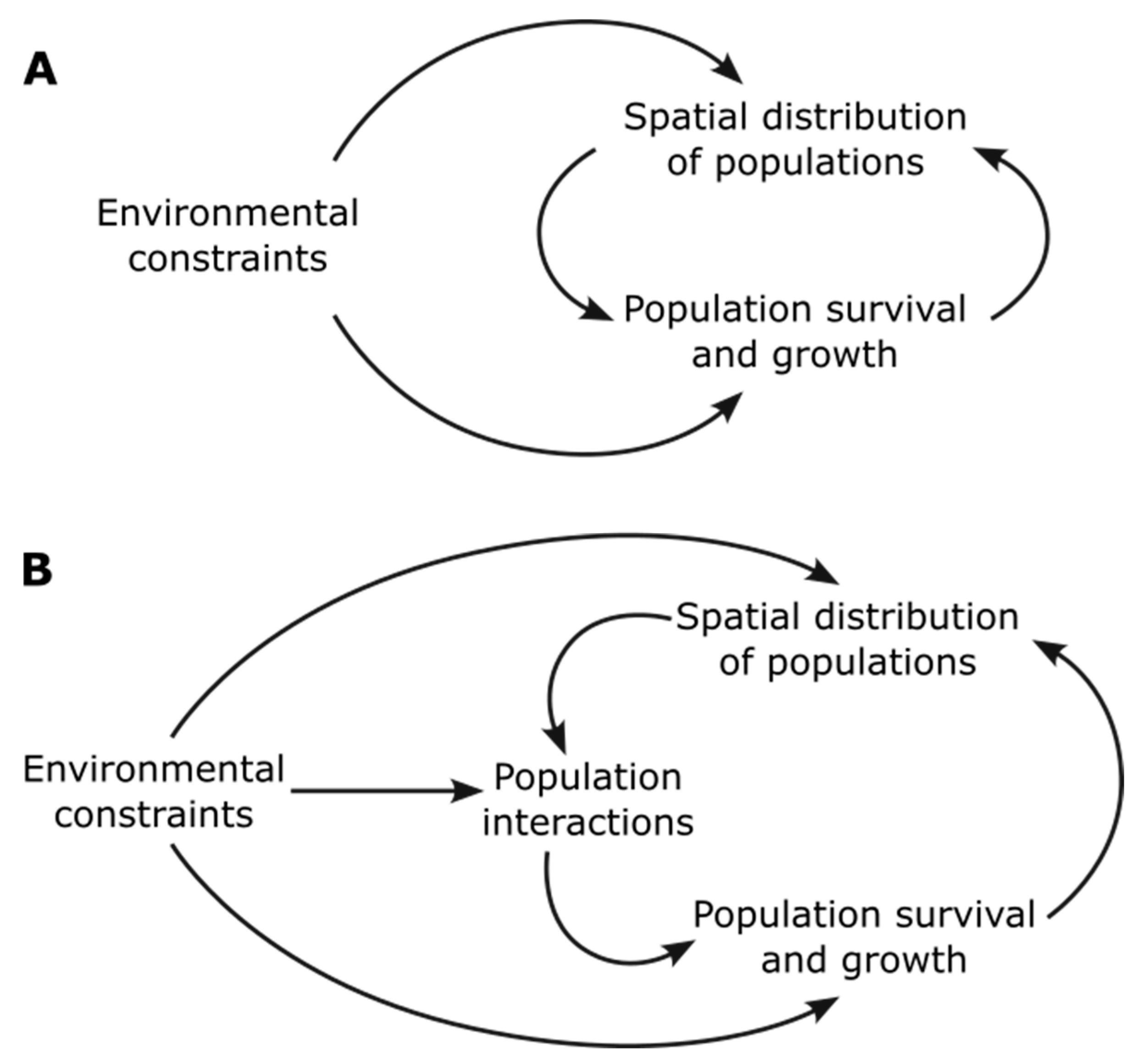
Figure 2.
Abiotic and biotic spatial heterogeneity affects the spatial distribution of microbial populations. As representative examples, abiotic spatial heterogeneity is experienced by (A) soil microbes in water channels around soil particles, (B) commensal bacteria colonizing skin glands and hair follicles, and (C) pathogenic bacteria and archaea at the site of a skin wound. Biotic forces can also make the environment heterogeneous, for example by (D) accumulation of progeny in the vicinity of parent cells due to slow dispersal or (E) creation of environmental gradients from species activities such as production of a diffusible metabolite.
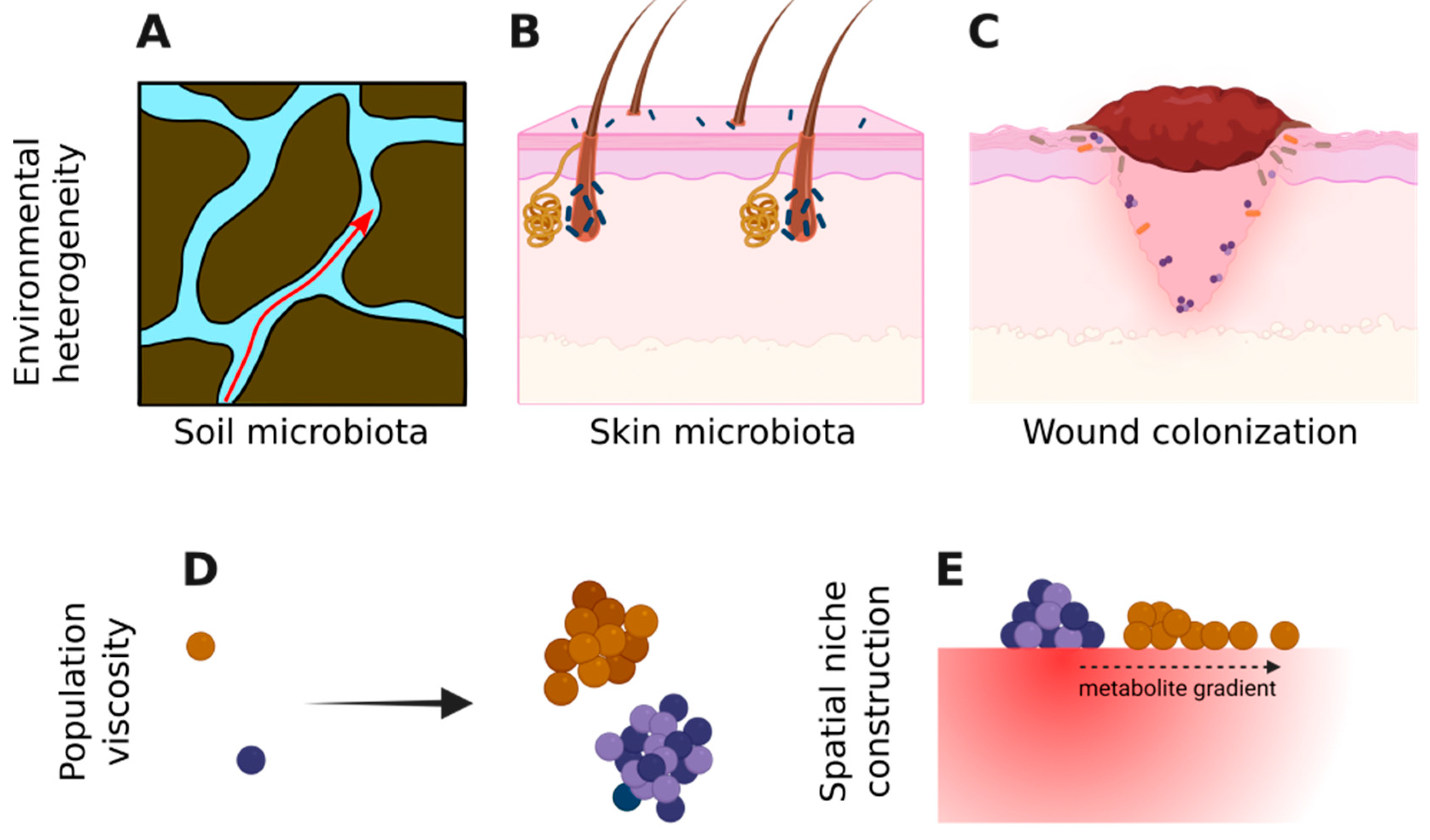
Figure 3.
When spatial self-organization drives population distributions within a community, the effective strength of interpopulation interactions will change. In mutualism (top), since each population grows better in the vicinity of the partner population, over time the populations become more spatially associated and the effective mutualism interaction becomes stronger. In antagonism (bottom), each population grows poorly in the vicinity of the partner, thus the populations become more segregated over time and the effective antagonism interaction becomes weaker.
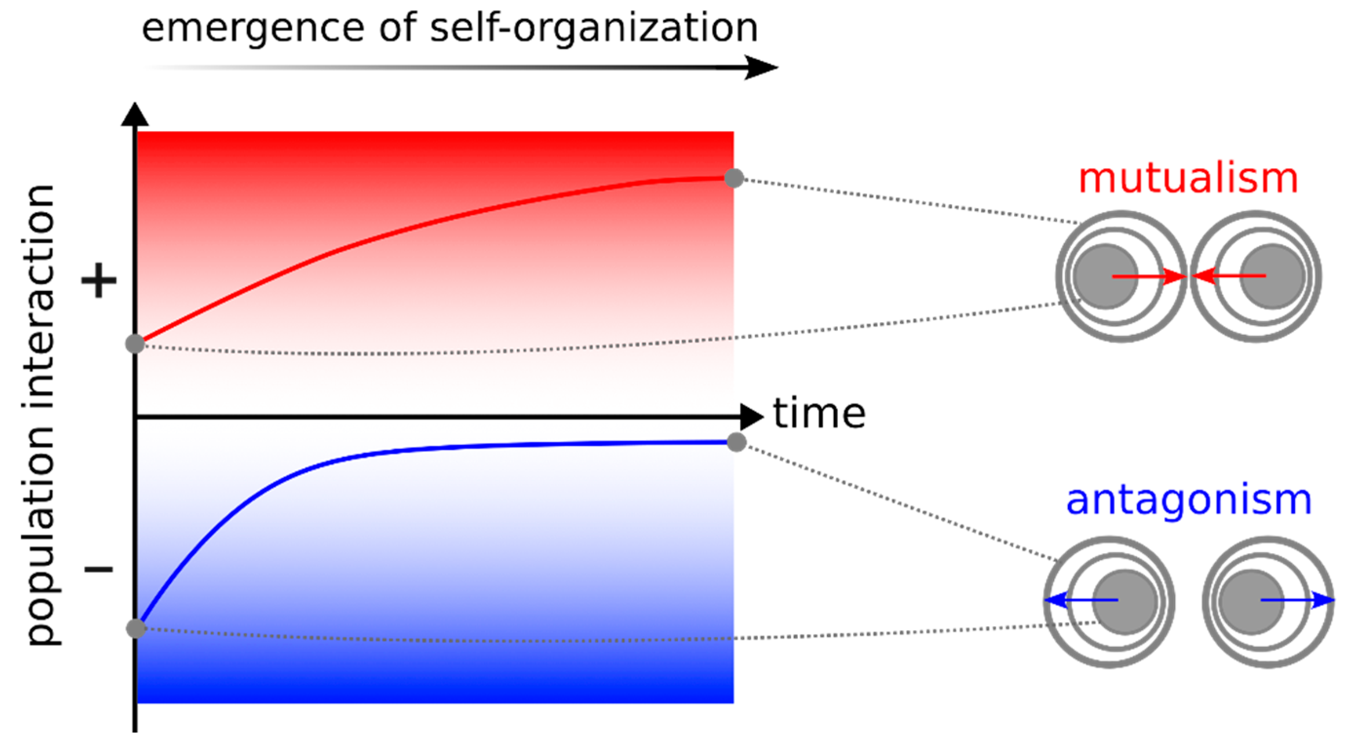
Figure 4.
Spatial self-organization can impact coexistence by changing the effective strength of interactions. Spatial self-organization is expected to strengthen facilitation (both for self and others) and self-inhibition, but to weaken the inhibition of other populations. Given that self-facilitation and other-inhibition are expected to disrupt coexistence, overall, spatial self-organization is expected to disfavor coexistence by supporting self-facilitation and favor coexistence by supporting other types of interactions.
Disclaimer/Publisher’s Note: The statements, opinions and data contained in all publications are solely those of the individual author(s) and contributor(s) and not of MDPI and/or the editor(s). MDPI and/or the editor(s) disclaim responsibility for any injury to people or property resulting from any ideas, methods, instructions or products referred to in the content. |
© 2025 by the authors. Licensee MDPI, Basel, Switzerland. This article is an open access article distributed under the terms and conditions of the Creative Commons Attribution (CC BY) license (http://creativecommons.org/licenses/by/4.0/).
Copyright: This open access article is published under a Creative Commons CC BY 4.0 license, which permit the free download, distribution, and reuse, provided that the author and preprint are cited in any reuse.


