Submitted:
29 August 2025
Posted:
02 September 2025
You are already at the latest version
Abstract
Fluoroscopy (real-time X-Ray) images are used for monitoring minimally-invasive coronary angioplasty operations such as stent placement.
During these operations a thin wire called a guidewire is used to guide different tools such as the stent or a balloon in order to repair the vessels.
However, fluoroscopy images are noisy and the guidewire is very thin, practically invisible in many places, making its localization very difficult.
Guidewire segmentation is the task of finding the guidewire pixels, while guidewire localization is the higher level task aimed at finding a parameterized curve describing the guidewire points.
This paper presents a method for guidewire localization that starts from a guidewire segmentation, from which it extracts a number of initial curves as pixel chains and uses a novel perceptual grouping method to merge these initial curves into a small number of curves.
The paper also introduces a novel guidewire segmentation method that uses a residual network (ResNet) as a feature extractor and predicts a coarse segmentation that is refined only in promising locations to a fine segmentation.
Experiments on two challenging datasets show that the method outperforms existing segmentation methods such as Res-UNet and nnU-Net, while having no skip connections and a faster inference time.
Keywords:
fluoroscopy
; guidewire segmentation
; guidewire localization
1. Introduction
Heart disease is still the number one cause of death in the US, accounting to 22% of the deaths in 2023 [1]. Heart disease is caused in main part by atherosclerosis, in which cholesterol deposits line the heart arteries, in time occluding them and starving the heart of oxygen. Currently there exists no medication to reverse atherosclerosis, only medication to prevent heart attacks and strokes.
The occluded arteries can be repaired either via bypass surgery, an invasive procedure that stops the heart and bypasses the clogged arteries, or by coronary angioplasty, a minimally invasive procedure that places stents (little specialized springs) at the occluded locations to keep the arteries open. The coronary angioplasty procedure is performed through catheters inserted in the body through an artery, and is monitored using real-time X-ray called fluoroscopy.
Inside the catheter is a thin wire called the guidewire that is used to penetrate the occluded location and guide different tools such as a stent or a balloon to perform the procedure. Because X-rays are harmful in high doses, the energy and duration of the X-ray is kept to a minimum, which results in noisy images and decreased guidewire visibility.
Finding the guidewire automatically is important for different purposes such as image augmentation, 2D-3D integration, etc. However, there are different levels of finding the guidewire.
The lowest level is guidewire segmentation, where just the pixels of the guidewire are desired to be found. A higher level task is guidewire localization, where a parametrization of the guidewire is desired to be found, either as a spline or another parametrized curve representation. This task is especially challenging because there might be multiple guidewires present in the image, and a separate curve is required for each of them. At the same time, because of the noisy nature of the fluoroscopy images, large parts of the guidewire might be invisible and seemingly disparate guidewire segments need to be combined into the same curve based on good continuation.
Finding a parameterization of the guidewire is important for certain tasks such as guidewire tracking or 2D/3D registration.
For this purpose, the paper brings the following contributions:
- (1)
- It introduces a guidewire segmentation method that uses two prediction outputs from a residual network or other feature extractor: one that that predicts a coarse segmentation directly from the encoder output, and one that refines the coarse segmentation only at the relevant places using a single convolutional layer. In contrast to the UNet or other segmentation methods, this architecture does not have any skip connections, making is simpler and faster to train.
- (2)
- It introduces a method for guidewire localization based on perceptual grouping of the curves extracted from the guidewire segmentation output. The novel perceptual grouping method uses a continuity measure to score what curves might belong to the same guidewire and the Hungarian algorithm to match the curve ends for grouping.
- (3)
- It performs experiments on two datasets, showing that the proposed segmentation outperforms other existing segmentation methods including the Res-UNet [2], a UNet with residual layers, and the nnU-Net [3], a well-celebrated segmentation method that is the state of the art for many medical imaging segmentation problems.
- (4)
- It also performs localization experiments and extensive ablations on the same datasets, showing that the proposed perceptual grouping obtains state of the art localization results with a small average number of curves per image.
2. Related Work
While there are quite a lot of work in guidewire segmentation, we are only aware of a small number of works on guidewire localization.
2.1. Guidewire Segmentation
The UNet [4] is a U-shape CNN architecture that has an encoder-decoder structure. The encoder has convolutional blocks followed by max-pooling to gradually reduce the spatial resolution of the output while increasing the number of channels. The decoder has mirror architecture with the encoder, with same number of blocks and uses skip-connections to bring information from the corresponding encoder layer, which are combined with the upscaled inputs from the previous block using convolutions.
The Res-Unet [2] is a modified UNet that was introduced for catheter segmentation. As opposed to the standard UNet that uses convolutions for the encoder and decoder blocks, [2] uses residual blocks [5], which are convolutional layers that sum the input to the block output for improved back-propagation.
A simple method based on image processing was introduced in [6] for guidewire segmentation and localization. The segmentation is obtained by applying a Frangi filter [7] and using a k-nearest neighbor classifier to classify pixel patches centered at high response locations and oriented by the Frangi filter orientation. The method is evaluated only on 8 image sequences and successfully detects the guidewire in 83.4% of the frames.
A steerable CNN was introduced in [8] as first level of screening for guidewire segmentation, where the CNN’s filters were steered to align with the guidewire direction for better accuracy. The paper used pixel patches for predicting the whether the center pixel is on the guidewire or not, and was focused on obtaining a good precision for 90% recall. In contrast, the proposed segmentation method uses a fully convolutional ResNet that takes a much larger context into account and is able to obtain a much better guidewire segmentation results that trade-off precision and recall.
A version of UNet was used in [9] for catheter segmentation. The method used a small UNet and transfer learning from synthetic data or phantom data, to obtain results similar to [2] on a catheter dataset.
In [10] the authors propose a two-phase guidewire segmentation method that uses a neural network to predict a binary indicator whether overlapping patches contain the guidewire or not, and a UNet to obtain the segmentation result on the patches that are predicted positive. The paper does not specify how to combine the obtained overlapping segmentations, and also misses details on data augmentation during training, and has no code available. In contrast, the guidewire segmentation part of our work uses a single neural network to predict at the same time a binary indicator on non-overlapping patches and to obtain the final segmentation on the predicted positive patches, without any UNet-like decoder and without any skip connections. Moreover, our architecture is fully convolutional and does not need to extract image patches, gathering larger context and obtaining much better segmentation results, besides being more computationally efficient.
Another UNet architecture with 12 transformer layers in the bottleneck was used in [11] for guidewire segmentation. However, the method was evaluated only on 11 image sequences and instead of segmenting the whole guidewire, the paper only segments the guidewire tip, which is much more visible. Moreover, the method cannot be reproduced due to missing important training details, such as the training loss function, data augmentation information, and there is no code available. The authors’ follow-up paper [12] introduces a background residual attention layer and multiple frames to obtain even better guidewire tip segmentation results, but the paper has the same reproducibility issues.
Another vision transformer has been used in [13] together with a shape sensitive loss function to improve the segmentation accuracy for many standard CNN architectures such as UNet [4], TransUNet [14], SwinU-Net [15], etc. This work is complementary to our work since it introduces a loss function, while our work introduces a novel architecture that is not a UNet. The shape sensitive loss could be also used in principle together with our architecture to further increase accuracy.
From the guidewire segmentation papers discussed in this section, one could see that that the segmentation results vary a lot from dataset to dataset. This is probably due to the variability introduces by the fluoroscopy machines, X-Ray intensity, sensor sensitivity, etc., as well as the quality of the annotation. Therefore, in our opinion, guidewire segmentation methods cannot be compared if they are evaluated on different datasets. They can only be compared on the same dataset using the same evaluation measure. Actually, [16] has pointed out that the same conclusion applies to many other medical image segmentation tasks.
In that respect, [17] introduced the CathAction dataset, a dataset of more than 23,000 of X-ray images obtained on endovascular interventions on pigs and phantoms. This dataset together with a more challenging guidewire dataset will be used in experiments to evaluate the proposed method and compare it with the state of the art.
2.2. Guidewire Localization
A hierarchical method for guidewire localization was introduced in [18]. The method first detects short segments on the guidewire using a trained object detector. The segments are used as nodes in a weighted graph, where the edge weighs are obtained by another classifier. Finally, a curve is obtained as the shortest path in the graph, thus a single curve is obtained for each image. In contrast, the proposed approach uses a deep CNN to obtain a good segmentation, from which initial curves are extracted, which are linked using a matching algorithm and a continuity measure.
Besides the Res-UNet segmentation method described in Section 2.1,2] also introduced a catheter localization method that extracts a centerline using skeletonization and connected components. The extracted curves are merged into a single curve using heuristics. Our proposed localization method also extracts centerlines using a type of skeletonization, but it constructs the curves as maximal chains of degree two nodes instead of connected components, which insures that each obtained curve is a chain of pixels with no bifurcations. Moreover, our method uses the Hungarian algorithm and a measure of curve continuation for merging the curves and the final number of curves is obtained automatically.
The k-NN based method [6] connects the segmented guidewire blocks using a greedy energy minimization algorithm that tries to minimize the sum of distances and the cosine of angles between the connected blocks.
3. Method Description
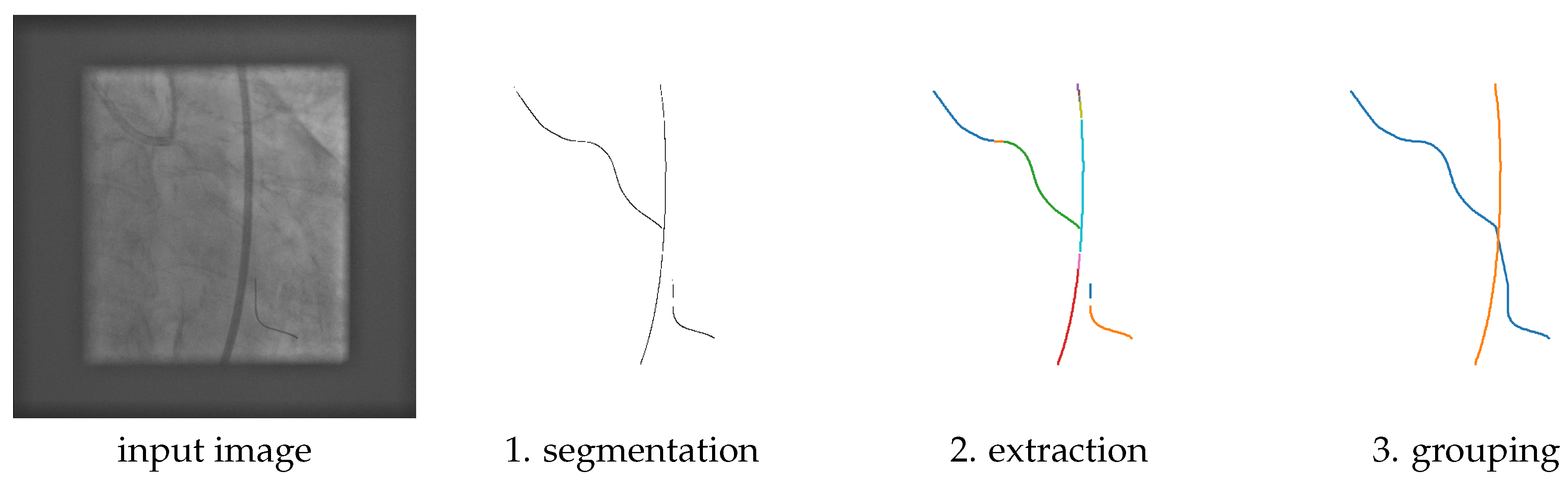
The proposed guidewire localization method is composed of four steps:
- (1)
- Guidewire segmentation, which labels the image pixels whether they belong to the guidewire or not.
- (2)
- Initial curve extraction, which takes the segmentation result and returns a number of pixel chains as initial curves.
- (3)
- Perceptual curve grouping, which merges the initial curves into longer curves based on a continuation measure.
- (4)
- Cleanup, an optional step that removes all obtained curves that are shorter than in length.
The first three steps are illustrated in Figure 1, and will be described in the following subsections.
Figure 1.
Example output obtained after each step of the proposed method on a test image. Each curve is shown in a different color.
Figure 1.
Example output obtained after each step of the proposed method on a test image. Each curve is shown in a different color.
3.1. Guidewire Segmentation
This step uses a deep CNN to obtain a good guidewire segmentation. The quality of the segmentation will be reflected in the quality of the obtained localization result, which is why we aim for the best possible segmentation.
For that reason, we introduce a novel segmentation method called MSLNet, described below.
3.1.1. Proposed MSLNet Segmentation Architecture
The proposed guidewire segmentation architecture is illustrated in Figure 2. It contains a ResNet (or other type of) feature extractor ) and two convolution filters, of size and of size , with in our experiments.
Figure 2.
Diagram of the proposed MSLNet guidewire segmentation architecture.
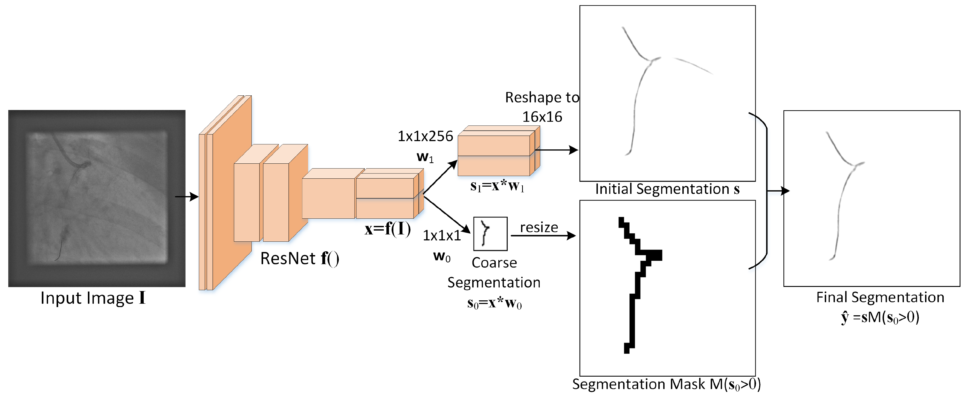
The MSLNet segmentation method consists of the following steps:
- (1)
- From an image of size , the ResNet is used as an encoder to extract a feature map of size with .
- (2)
- An initial segmentation is obtained from the feature map using the convolution kernel , which produces a map of size . Each dimensional vector from this map is reshaped to a patch and placed at the corresponding location in a grid of patches, which together form the initial segmentation of size .
- (3)
- From the feature map , a coarse segmentation of size is also obtained using the convolution kernel .
- (4)
- The final segmentation is obtained as , where is the indicator function and resizes the input to make it z times larger in each direction, without interpolation, thus
The whole process is summarized in Algorithm 1 below, where the number of channels used in this paper is .
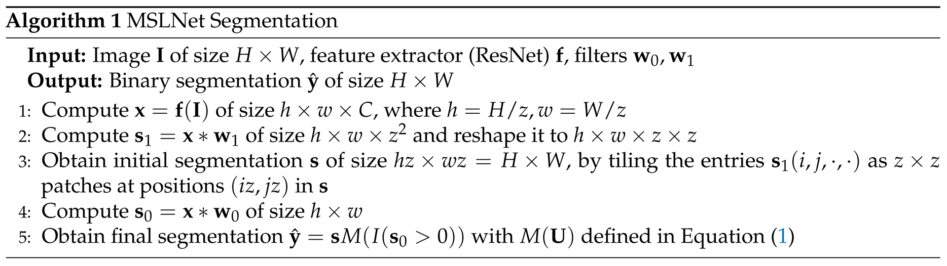
Observe that this approach requires the input image dimensions to be divisible by z. If that’s not the case, the image is padded with zeros to make it divisible.
It is worth noting that this architecture directly predicts the segmentation from the encoded representation without many decoder layers and without skip connections. This reduces the number of trainable parameters and the depth of the CNN, but faces some overfitting issues that are addressed by the coarse segmentation branch .
This approach can be thought as a Marginal Space Learning (MSL) approach [18,19], where the marginal space is the space of coarse segmentations , which is times smaller than the final segmentation space. Only the patches corresponding to locations where are expanded to a fine segmentation, the rest are just set to zero. This is the reason why this approach is called MSLNet.
3.2. Training the MSLNet
Training is done end-to-end using a two-term loss function that encourages a good coarse segmentation and a good final segmentation . This is in contrast with [10], where the coarse segmentation and the UNet are trained separately.
The trainable parameters consist of the ResNet feature extractor parameters and the two convolution kernels .
Given a training example with input and target binary segmentation , the coarse target is first constructed as a binary indicator for the grid of patches whether they contain at least one guidewire pixel:
After constructing , the training loss function for an observation has two parts,
the coarse segmentation loss and the fine segmentation loss , where is the ResNet feature extractor and ’*’ is the convolution operator.
Inspired by [3], who combine the Dice and BCE losses, the coarse segmentation loss is the sum
of the Dice loss and the weighted BCE loss. The Dice loss is
where the sums are taken over the coarse pixels, the function is the sigmoid, and is a tuning parameter ( in our experiments).
The weighted binary cross-entropy (BCE) loss is
where are the positive pixels of the coarse target and are the negative ones.
The fine segmentation loss is also the sum of the Dice loss and the weighted binary cross entropy (BCE) loss:
where here and with as defined in Equation (1).
By restricting the fine segmentation loss only to patches where , we make sure that the training data is more balanced, since in this case the percentage of foreground pixels is about , as opposed to when considering the entire image when the percentage of foreground pixels is about .
However, due to inaccuracies in the annotation, the BCE fine segmentation loss might not be the best choice because it is not very robust to labeling noise. For that reason, we also experimented replacing with the Lorenz loss [20]:
where is the ReLU and are the same as for Equation (7). This loss is more robust to labeling noise because it penalizes a mistake less than the BCE loss.
3.3. Initial Curve Extraction
To extract the initial curves, the thresholded segmentation result is processed using the thinning morphological operation so that each pixel of the obtained output has a small number of neighbors, enabling the extraction of the initial curves as pixel chains. Thinning [21] is an iterative morphological algorithm that is applied to a binary image until convergence, and aims to find the centerline of a strip of pixels. In our experiments, we used Matlab’s bwmorph with the thinning option and scikit-image’s thin with identical results. We also experimented with two other related morphological operations: skeletonization and medial axis, but observed that thinning obtained slightly better results.
To extract the pixel chains as curves, first the 8-neighbor graph is constructed with V as the positive pixels of the thinned segmentation. On the thinned segmentation result, most nodes of this graph have degree 2 and some have degree 3. Nodes with degrees more than 3 are very rare.
The rest of the curve extraction is described in Algorithm 2 below.
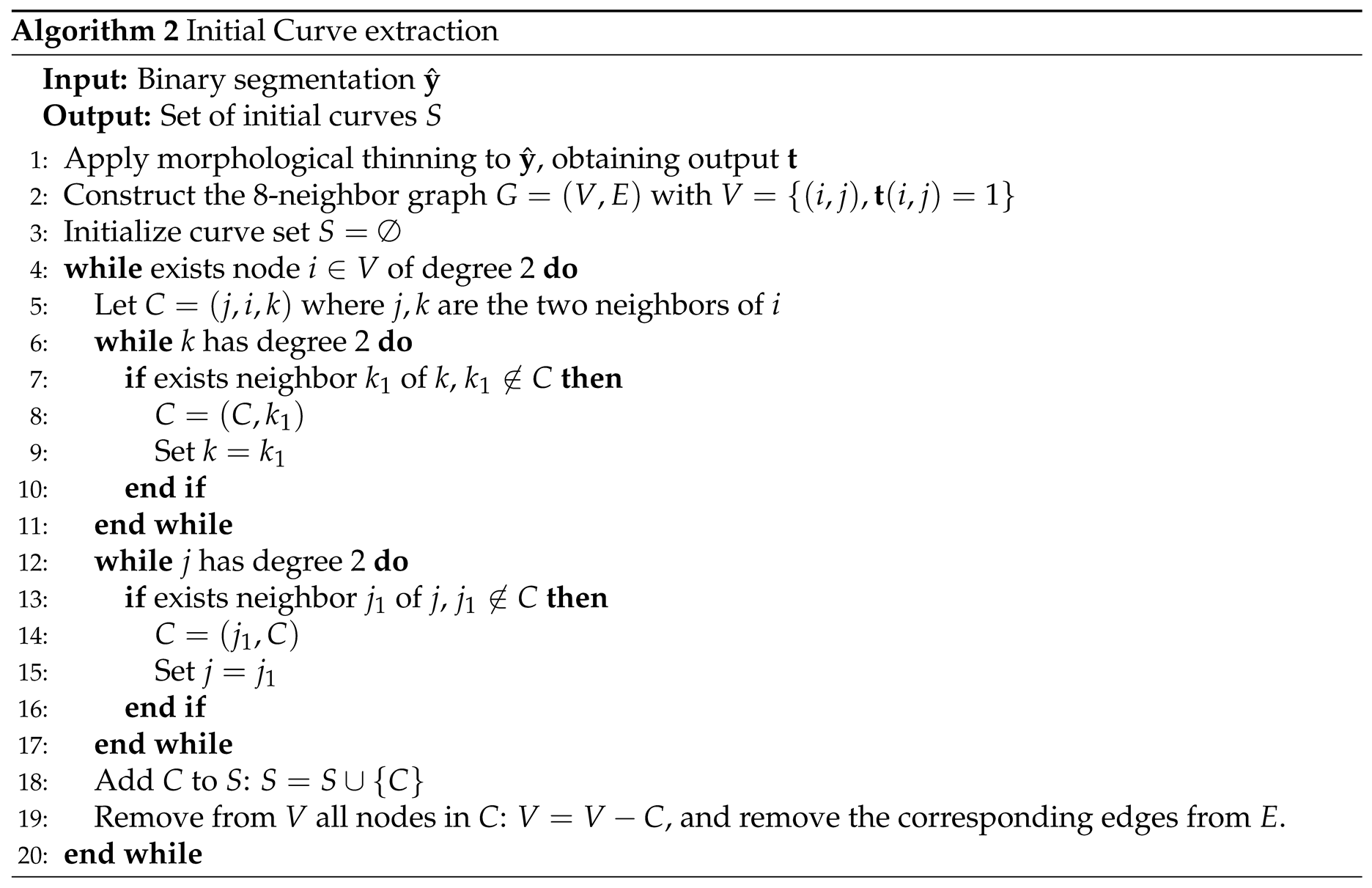
Lines 6-17 extract the initial curves as maximal chains C containing a node i of degree 2. Observe that because it is a chain, each curve C induces an ordering of its nodes, ordering that is unique up to its reversal.
3.4. Perceptual Curve Grouping
Perceptual curve grouping takes the curves extracted in sec:extract and merges them into longer curves using a continuation measure. When two curves are merged, the pixel ordering for one of them might need to be reversed to obtain a consistent ordering for the merged curve. The whole perceptual grouping algorithm is described in Algorithm 3, with its components being described below.
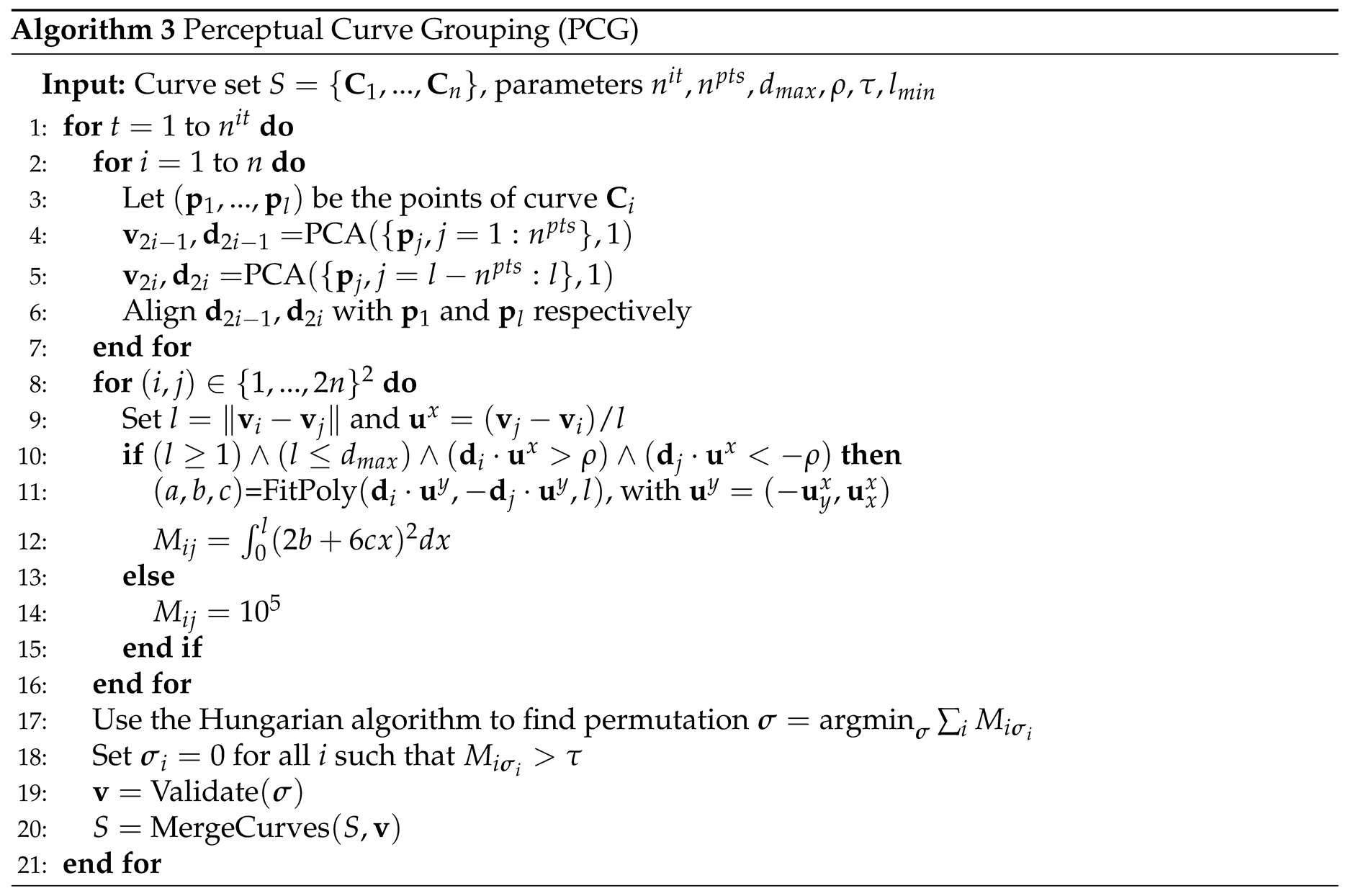
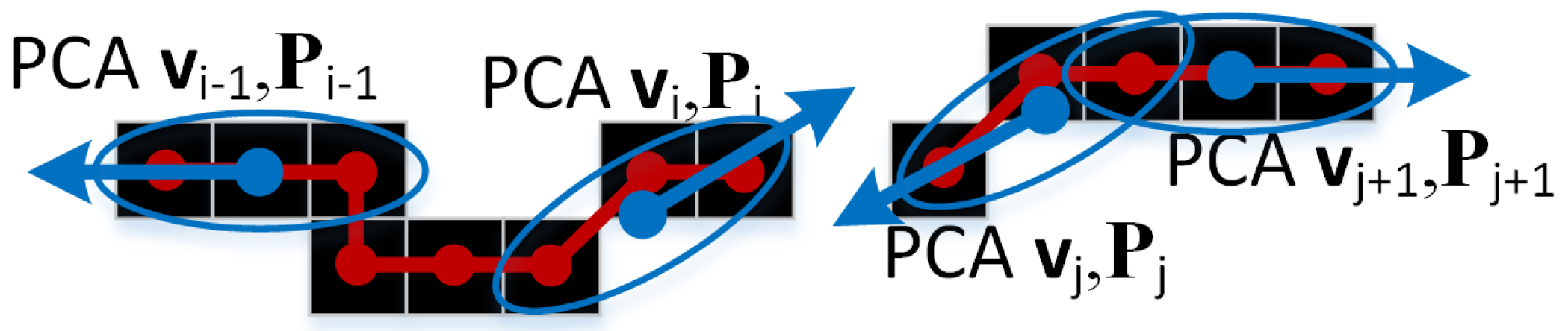
In Algorithm 3, end curve directions are estimated using PCA for each curve, and are used for the curve continuation measure.
So, for n curves, there are PCA models, with models and corresponding to curve . Model is built from the first k points of the curve, as illustrated in Figure 3, while model is built from the last k points. If the curve is less than k points long, the PCA models are estimated from all curve points. We used in experiments.
Figure 3.
The end curve models are PCAs constructed from the first and last pixels of each curve (shown as blue ellipses) and aligned to point outwards from the curve.
Figure 3.
The end curve models are PCAs constructed from the first and last pixels of each curve (shown as blue ellipses) and aligned to point outwards from the curve.
The directions are then aligned in step 6 to point outwards from the curve by making them point towards the respective end of the curve. To align a direction with mean to point towards , first is computed. If , then is already aligned. If , then the direction is reversed: .
The point-direction pairs are checked in line 10 to be within a distance range and an angle alignment. The angle alignment checks that the angles between and , and between and , are less than , corresponding to in line 10 of alg:grouping.
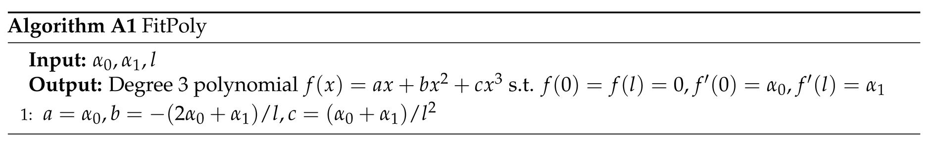
For the pairs that pass the check, a continuation measure is computed as based on fitting a degree 3 polynomial , as specified in alg:poly and illustrated in Figure 4.
Figure 4.
A degree 3 polynomial is fitted between the points and on the coordinate system with the x-axis connecting the two points.
Figure 4.
A degree 3 polynomial is fitted between the points and on the coordinate system with the x-axis connecting the two points.
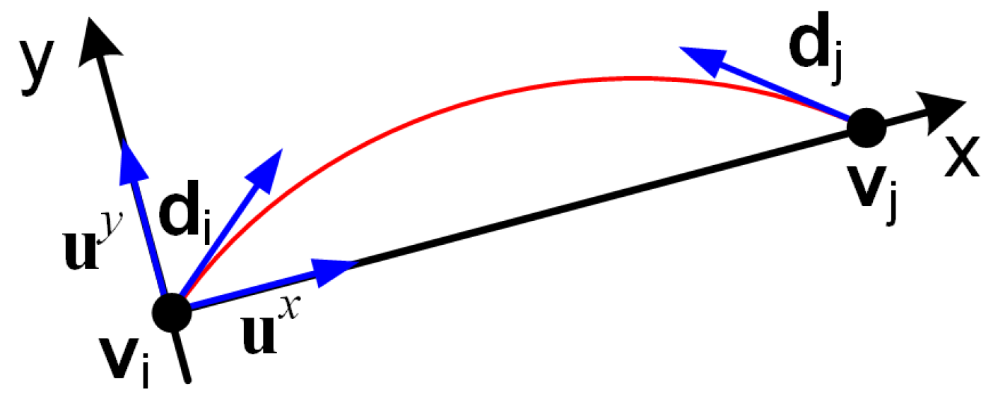
For that, a coordinate system is constructed, centered at with x-axis towards , thus the x-axis is and the y-axis is .
Then a degree three polynomial is fitted analytically to go through and be tangent to as described in alg:poly. One can easily check that , so the continuation matrix M is symmetric.
The curve ends are matched using the Hungarian algorithm [22] and the matches with cost are discarded.
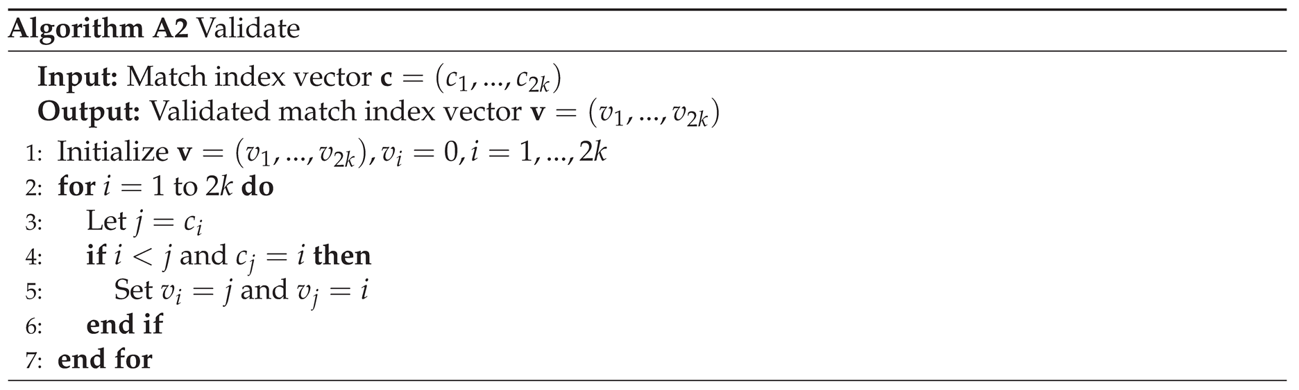
The matches are validated so that only pairs such that i is matched to j and j is matched to i are kept, as described in alg:validate. This step is essential, since the curve merging step would fail without it.
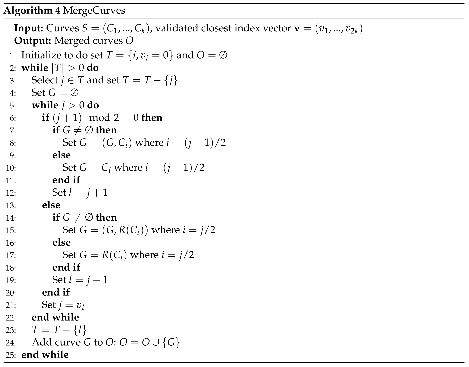
Then the curves are merged based on the validated endpoint matches, as described in Algorithm 4. The function reverses the points of a curve C.
4. Experiments
Experiments are performed on two datasets: a guidewire dataset and the CathAction dataset [17].
The guidewire dataset contains 82 fluoroscopic video sequences recorded during coronary angioplasty procedures with 871 frames of various sizes in the range . Of the 82 video sequences, 42 were used as training data, containing 433 frames, and 40 as test data containing 438 frames. Two example images from this dataset are shown in Figure 1 and Figure 2.
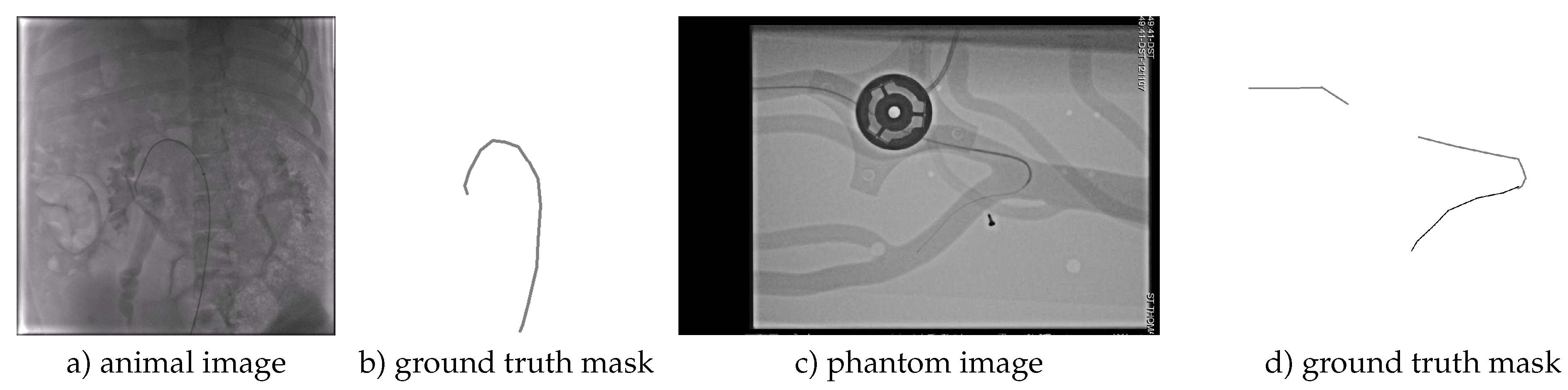
The CathAction dataset [17] contains 23449 X-ray images obtained from endovascular interventions on animals (pigs) and imaging phantoms. The CathAction dataset divides the images into 18758 training images consisting of 4021 animal and 14737 phantom, and 4691 test images with 1006 animal and 3685 phantom frames. The dataset is annotated for segmentation, with the catheter pixels and guidewire pixels annotated with different labels, with two examples shown in Figure 5. As one can see, the guidewire is not annotated inside the catheter and the catheter is approximated with long line segments, so the annotation is not very precise. The annotation is 3-5 pixels thick.
Figure 5.
Example images from the CathAction dataset and their corresponding ground truth masks.
4.1. Methods Compared and Implementation Details
For segmentation, we compared our proposed MSLNet segmentation approach with the nnU-Net [3], the ResUNet [2], the SCNN [8], the two step method from [10], and the hierarchical method from [18].
For localization, we compared with the hierarchical localization [18], and with [2], as these two were the only methods that output parameterized curves.
For nnU-Net we used the GitHub package https://github.com/MIC-DKFZ/nnU-Net, and trained it on our data using the default parameters except the number of epochs was 300. Ensembling was not used, for a fair comparison.
The MSLNet was also trained as part of the NN-UNet framework, for better segmentation results, because the NN-UNet framework offers a rich array of data augmentation transformations that were proven to be useful in many segmentation applications [16].
For the Res-UNet [2] architecture, we used the authors’ code from the GitHub package https://github.com/pambros/CNN-2D-X-Ray-Catheter-Detection, but trained it within the NN-UNet framework, again for better segmentation results. We also used the authors’ curve grouping code from the same GitHub package to obtain the localization results.
Because the two step method [10] does not have code available, we used our own implementation of the classification CNN and the segmentation UNet based on the description in the paper. However, we encountered overfitting issues when training these models without data augmentation. For the UNet, without data augmentation, the train was 0.78 and the test was 0.26 on the guidewire dataset. With data augmentation, the train was 0.36 and the test was 0.26. For the binary classification CNN, data augmentation in the form of random translation up to 4 pixels and random rotation up to 15 degrees helped with overfitting, obtaining a train of 0.90 and a test of 0.46 on the guidewire dataset.
For the SCNN [8] we used our own implementation of a four-layer SCNN, and for the Hierarchical method [18] we used a pretrained model.
All experiments were performed on a Core I7 computer with 32 GB Ram and a NVIDIA GeForce 3090 GPU.
The training and test times for the different methods on the guidewire dataset are summarized in Table 1, where the test times and the FLOPS are shown for 512×512 images. From Table 1 one could see that the MSLNet has the smallest detection time, due to the fact that the ResNet feature extractor is a fully convolutional network, so it can be applied directly to images of any size. The other competitive methods such as NN-UNet and Res-UNet need to crop images of a certain size on which to apply the segmentation, and then to merge the obtained results into a final segmentation output, which increases the segmentation time.

4.2. Evaluation Measures
The methods are evaluated using precision, recall, scores, Dice coefficient and IOU (Intersection over Union). Because some methods only obtain a segmentation, separate comparisons are conducted for segmentation and for localization. All results are shown as the average and standard deviation obtained from four independent runs, except for the Hierarchical method from [18], for which we only have a pretrained model.
Annotating a one-pixel wide guidewire is prone to inaccuracies, which can drastically affect standard measures such as the Dice coefficient or IOU . To see that, one can imagine evaluating a perfect 1-pixel wide result with a 1-pixel wide annotation that is one pixel off everywhere. Such a result would have a Dice and IOU of 0, while being visually close to perfect. Our conclusion is that Dice and IOU are very good for evaluating blob-like structures such as organs, but not for very thin structures such as the guidewire. The catheter segmentation evaluation is somewhere in the middle, be because the catheter is 3-5 pixels wide, so the Dice and IOU are less sensitive than for the guidewire evaluation, but they are still sensitive to some extent.
For this reason, besides the Dice and IOU, we will also evaluate using precision, recall and scores measures that are specifically designed for robustness to such inaccuracies. The precision is defined as the percent of detected pixels that have an annotated guidewire or catheter pixel at a distance of at most 3 pixels. The recall is defined as the percent of guidewire pixels that are at a distance at most 3 from a detected pixel. The score is defined as usual, , in terms of the precision p and the recall r defined above.
On the CathAction dataset, the mask annotation is usually several pixels thick, but the method from [18] always outputs a one-pixel wide result, so the Dice and IOU results are even less relevant for this method on this dataset.
For guidewire localization, the same precision and recall measures are used to evaluate the rasterization of the obtained curves. However, for the CathAction dataset, which does not provide a one-pixel wide annotation but a several pixels wide segmentation, the annotation is first thinned to approximate the location of the guidewire inside the catheter and this thinned segmentation is used to compute the recall. The localization Dice and IOU are also evaluated on this thinned segmentation to be able to compare one-pixel wide results with one-pixel wide annotations. The guidewire localization is also evaluated on the average number of curves obtained per image, which is desired to be close to the true average number of curves, obtained from the annotation, which on the guidewire test set is 1.1. We don’t know the average number of curves on the CathAction dataset because the dataset does not provide curve annotations, only segmentation masks. Approximating the number of curves using connected components on the CathAction GT masks, we obtained an average of 1.4 curves per image on the test set. However, this might not be an accurate number as one could see in Figure 5, d), where there is only one catheter but the GT mask is broken into two connected components.
4.3. Segmentation Results
The segmentation results are displayed in Table 2 for both datasets. Two sample t-tests based on the results on the four independent runs runs were conducted to compare the best results with the other ones, except the Hierarchical method [18], which is quite behind anyway. Based on these t-tests, the best results and the ones that are not significantly worse () are shown in bold.
Table 2.
Segmentation results. Shown are the mean (and std) obtained on the test set from four independent runs.
Table 2.
Segmentation results. Shown are the mean (and std) obtained on the test set from four independent runs.
| Method | Precision | Recall | Dice | IOU | ||
|---|---|---|---|---|---|---|
| Guidewire dataset | ||||||
| Hierarchical [18] | 94.80 | 57.14 | 71.30 | 19.25 | 11.00 | |
| SCNN [8] | 44.86 (1.31) | 62.15 (0.78) | 52.09 (0.62) | 18.67 (0.11) | 10.71 (0.06) | |
| Two phase [10] | 28.18 (2.12) | 70.74 (3.59) | 40.22 (2.18) | 15.45 (1.22) | 8.63 (0.77) | |
| Res-UNet[2] | 94.30 (0.99) | 69.50 (0.13) | 80.02 (0.33) | 40.17 (0.26) | 26.53 (0.20) | |
| nnU-Net [3] | 98.18 (0.35) | 73.47 (0.89) | 84.04 (0.54) | 41.51 (0.67) | 27.22 (0.54) | |
| MSLNet | 98.25 (0.22) | 81.98 (0.45) | 89.38 (0.29) | 45.06 (0.11) | 30.05 (0.10) | |
| MSLNet-Lor | 97.16 (0.24) | 88.60 (0.46) | 92.68 (0.20) | 48.82(0.03) | 33.00 (0.02) | |
| CathAction dataset | ||||||
| Hierarchical [18] | 56.13 | 42.23 | 48.20 | 11.92 | 6.55 | |
| SCNN [8] | 70.68 (0.19) | 70.32 (1.18) | 70.50 (0.67) | 17.01 (0.26) | 9.37 (0.15) | |
| Two phase [10] | 50.24 (3.57) | 93.49 (0.21) | 65.28 (2.94) | 36.71 (2.15) | 23.54 (1.65) | |
| Res-UNet [2] | 91.33 (0.13) | 93.66 (0.03) | 92.48 (0.08) | 62.07 (0.05) | 46.13 (0.07) | |
| nnU-Nnet [3] | 91.46 (0.30) | 93.82 (0.47) | 92.62 (0.15) | 62.19 (0.18) | 46.25 (0.20) | |
| MSLNet | 91.52 (0.10) | 94.62 (0.13) | 93.05 (0.02) | 62.51 (0.04) | 46.58 (0.04) | |
| MSLNet-Lor | 87.36 (0.20) | 97.74 (0.06) | 92.26 (0.09) | 60.45 (0.14) | 44.04 (0.15) | |
Two MSLNet versions are shown, with "MSLNet" being trained with the Dice+BCE loss function from Equation (7), and "MSLNet-Lor" being trained with the Dice + the Lorenz loss from Equation (8).
From Table 2, MSLNet performs better than the other methods, including the nnU-Net. The Lorenz loss has a strong influence on the results for the guidewire dataset, where the wire is one pixel wide, increasing the score from 89.38 to 92.68, but not for the CathAction dataset where the catheter is 3-5 pixels wide.
As expected, the nnU-Net [3] performed very well on both datasets, being the second best after MSLNet, followed by the Res-UNet [2]. The other three methods, SCNN[8], Two phase [10] and Hierarchical [18] are behind by a large margin. The Steerable CNN [8] was designed to only serve as an initial step towards segmentation, using patches to predict whether the center pixel is on the guidewire or not. For that reason it is not capable to capture long range interactions and it has scores comparable with the Two-phase method [10], which uses patches. Also because it uses a Spherical Quadrature Filter [23] response map as a preprocessing step, the output is one pixel thin, so the Dice/IOU scores for the CathAction data are very small and unreliable.
We can also see from Table 2 that some methods reach quite high scores around 90% while the Dice/IOU scores are very low. In our opinion, this serves as a confirmation that the Dice/IOU scores are more sensitive to annotation inaccuracies for the wire-like structures than the precision/recall and scores defined in Section 4.2. Moreover, we see that the Dice/IOU scores are higher on the CathAction data than on the guidewire data for some methods with similar scores of about . This is in line with the fact that the catheter that is evaluated in the CathAction data is thicker than the guidewire, so the Dice/IOU are less sensitive to annotation errors for the catheter than for the guidewire. Nevertheless, all three measures ( score, Dice and IOU) tell the same story about how the best segmentation methods compare with each other.
4.4. Localization Results
The localization results are shown in Table 3. From Table 3 one could see that the two MSLNet versions obtain the best results in all measures by a large margin, followed by Res-UNet [2] and then by the Hierarchical method [18].
Table 3.
Localization results. Shown are the mean (and std) obtained on the test set from four independent runs.
Table 3.
Localization results. Shown are the mean (and std) obtained on the test set from four independent runs.
| Method | Precision | Recall | Dice | IOU | Avg #curves | |
|---|---|---|---|---|---|---|
| Guidewire dataset | ||||||
| Hierarchical [18] | 94.80 | 57.48 | 71.56 | 18.79 | 10.68 | 1.0 (0.0) |
| Res-UNet [2] | 95.66 (0.82) | 60.62 (0.75) | 74.20 (0.39) | 34.30 (0.32) | 21.84 (0.27) | 1.0 (0.0) |
| MSLNet | 97.56 (0.14) | 82.52 (0.73) | 89.41 (0.41) | 37.29 (0.14) | 23.74 (0.09) | 1.3 (0.0) |
| MSLNet-Lor | 96.76 (0.20) | 88.19 (0.49) | 92.28 (0.22) | 37.00 (0.09) | 23.51 (0.06) | 1.3 (0.0) |
| CathAction dataset | ||||||
| Hierarchical [18] | 49.62 | 45.67 | 47.57 | 8.48 | 4.61 | 1.0 (0.0) |
| Res-UNet [2] | 56.88 (0.45) | 50.49 (0.75) | 53.49 (0.62) | 6.28 (0.12) | 3.33 (0.07) | 1.0 (0.0) |
| MSLNet | 85.65 (0.09) | 81.58 (0.14) | 83.57 (0.04) | 16.90 (0.07) | 9.53 (0.04) | 1.1 (0.0) |
| MSLNet-Lor | 84.93 (0.08) | 82.01 (0.05) | 83.44 (0.06) | 16.88 (0.03) | 9.51 (0.02) | 1.3 (0.1) |
Here the Dice and IOU scores are even less reliable because the results as well as the annotations are both 1-pixel wide (see examples in Figure A3 and Figure A4) and the Dice/IOU scores are extremely sensitive to even 1-pixel discrepancies between the annotation and the localization result.
Looking at the CathAction scores, we notice that the Res-UNet [2] curve grouping method starts with a good segmentation score of 92.48, and obtains a localization score of 53.49, while the MSLNet-Lor starts from a slightly smaller score of 92.26, obtaining a localization of 83.44. A similar but not so dramatic phenomenon is observed on the guidewire dataset. This is an indication that our proposed perceptual grouping method does a better job at grouping curves based on good continuation than the method from [2].
4.5. Segmentation Ablation Studies
The segmentation ablation studies evaluate the importance of using the MSL training, the form of the loss function for the coarse segmentation , and the form of the loss function for the fine segmentation.
The importance of MSL. In this experiment, we removed the coarse segmentation and its coarse loss function, so we just kept the upper path in Figure 2, so the final segmentation is the initial segmentation . The results using the Dice+BCE loss from Equation (7), with and without MSL are shown in Table 4. From Table 4 one could see that the MSL training is important for the guidewire dataset, but not for the CathAction dataset.
Table 4.
The influence of using the MSL training for segmentation accuracy.
| Dataset | MSL | Precision | Recall | Dice | IOU | |
|---|---|---|---|---|---|---|
| Guidewire | N | 98.78 (0.14) | 78.74 (0.38) | 87.63 (0.27) | 44.47 (0.39) | 29.71 (0.30) |
| Guidewire | Y | 98.25 (0.22) | 81.98 (0.45) | 89.38 (0.29) | 45.06 (0.11) | 30.05 (0.10) |
| CathAction | N | 91.27 (0.05) | 94.80 (0.11) | 93.01 (0.07) | 62.68 (0.04) | 46.76 (0.04) |
| CathAction | Y | 91.52 (0.10) | 94.62 (0.13) | 93.05 (0.02) | 62.51 (0.04) | 46.58 (0.04) |
The form of the coarse segmentation loss function . Intuitively, the course segmentation loss function should follow the pattern observed by [3], that the Dice+BCE loss is better for segmentation than the individual Dice or BCE losses. Indeed, Table 5 confirms this intuition, with the Dice+BCE loss obtaining higher scores than using the Dice or BCE losses for the guidewire dataset. However, the Dice scores are higher when using the Dice loss only, because in this case the Dice is explicitly maximized by that loss. But the higher Dice score is not reflected in a higher score, so we consider it as unreliable.
Table 5.
The influence of the form of the coarse segmentation loss function on the guidewire dataset.
Table 5.
The influence of the form of the coarse segmentation loss function on the guidewire dataset.
| Loss | Precision | Recall | Dice | IOU | |
|---|---|---|---|---|---|
| Dice | 97.04 (0.66) | 79.84 (0.80) | 87.60 (0.70) | 45.13 (0.57) | 30.14 (0.43) |
| BCE | 98.14 (0.17) | 80.30 (0.57) | 88.33 (0.39) | 44.19 (0.28) | 29.40 (0.21) |
| Dice+BCE | 98.25 (0.22) | 81.98 (0.45) | 89.38 (0.29) | 45.06 (0.11) | 30.05 (0.10) |
The form of the fine segmentation loss function . For the fine segmentation, we know from [3] that Dice+BCE is better than Dice or BCE alone, so we only compare the Dice+BCE from Equation (7) with Dice+Lorenz, where the Lorenz loss is given in Equation (8). The results are given in Table 6. From Table 6, one could see that the Lorenz loss is important for obtaining higher and Dice scores for the guidewire dataset which has 1-pixel wide annotations, but not for the CathAction dataset, which has thicker annotations.
Table 6.
The influence of the form of the fine segmentation loss function .
| Dataset | Loss | Precision | Recall | Dice | IOU | |
|---|---|---|---|---|---|---|
| Guidewire | Dice+BCE | 98.25 (0.22) | 81.98 (0.45) | 89.38 (0.29) | 45.06 (0.11) | 30.05 (0.10) |
| Guidewire | Dice+LOR | 97.16 (0.24) | 88.60 (0.46) | 92.68 (0.20) | 48.82 (0.03) | 33.00 (0.02) |
| CathAction | Dice+BCE | 91.52 (0.10) | 94.62 (0.13) | 93.05 (0.02) | 62.51 (0.04) | 46.58 (0.04) |
| CathAction | Dice+LOR | 87.36 (0.20) | 97.74 (0.06) | 92.26 (0.09) | 60.45 (0.14) | 44.04 (0.15) |
4.6. Localization Ablation Studies
The localization ablation evaluates the importance of the whole perceptual grouping algorithm and its tuning parameters in the quality of the localization result.
The importance of perceptual grouping. First, we evaluate the importance of the proposed perceptual grouping algorithm. For that, in Table 7 are shown localization results after initial curve extraction, with and without perceptual grouping on the guidewire dataset starting from the MSLNet-Lor segmentation. Also shown are results after the cleanup step of removing short curves (less than pixels) directly from the extracted curves, without perceptual grouping.
Table 7.
Ablation of the two main localization steps after curve extraction: perceptual grouping (PG) and cleanup (removing short curves) on the guidewire dataset. Shown are test set means (std) from four independent runs.
Table 7.
Ablation of the two main localization steps after curve extraction: perceptual grouping (PG) and cleanup (removing short curves) on the guidewire dataset. Shown are test set means (std) from four independent runs.
| Perceptual grouping | Cleanup | Precision | Recall | Dice | IOU | Avg #curves | |
|---|---|---|---|---|---|---|---|
| N | N | 97.24 (0.20) | 87.76 (0.44) | 92.26 (0.20) | 37.01 (0.09) | 23.52 (0.07) | 2.5 (0.0) |
| N | Y | 97.48 (0.21) | 86.61 (0.46) | 91.73 (0.25) | 36.83 (0.11) | 23.39 (0.07) | 1.6 (0.0) |
| Y | N | 96.76 (0.20) | 88.19 (0.49) | 92.28 (0.22) | 37.00 (0.09) | 23.51 (0.06) | 1.3 (0.0) |
| Y | Y | 96.88 (0.20) | 88.08 (0.53) | 92.27 (0.25) | 36.98 (0.11) | 23.49 (0.08) | 1.3 (0.0) |
From Table 7, one could see that the extracted initial curves are broken into many pieces, and just removing the short pieces results in a worse localization result with more curves than when using the proposed perceptual grouping method.
We can also see that cleanup after perceptual grouping has a minimal influence and the cleanup step can be removed.
Tuning parameters. The perceptual grouping method has a number of tuning parameters: the number of iterations , the number of points to estimate the endpoint directions , the maximum distance for endpoint matching, the minimum alignment parameter , the maximum continuity score and the minimum final curve length . They are set to the following values: .
The dependence of the obtained result on each of these parameters while the others are kept to the above values is shown in Table 8. These experiments are performed on the guidewire dataset starting from the MSLNet-Lor segmentation. From Table 8, one could see that the score and average number of curves depend only slightly on these parameters when their value is in the range from the table.
Table 8.
The influence of perceptual grouping parameters and in localization scores and average number of curves per image. The base segmentation is from MSLNet-Lor. Shown are test means (std) from four runs.
Table 8.
The influence of perceptual grouping parameters and in localization scores and average number of curves per image. The base segmentation is from MSLNet-Lor. Shown are test means (std) from four runs.
| 1 | 2 | 3 | 4 | |
|---|---|---|---|---|
| 92.28 (0.20) | 92.31 (0.22) | 92.28 (0.22) | 92.26 (0.22) | |
| Avg # curves | 1.5 (0.0) | 1.4 (0.0) | 1.3 (0.0) | 1.3 (0.0) |
| 3 | 5 | 10 | 20 | |
| 92.22 (0.27) | 92.10 (0.25) | 92.28 (0.22) | 92.27 (0.25) | |
| Avg # curves | 1.4 (0.0) | 1.3 (0.0) | 1.3 (0.0) | 1.4 (0.0) |
| 10 | 20 | 40 | 50 | |
| 92.03 (0.31) | 92.29 (0.20) | 92.28 (0.22) | 92.26 (0.22) | |
| Avg # curves | 1.5 (0.0) | 1.4 (0.0) | 1.3 (0.0) | 1.3 (0.0) |
| 0.3 | 0.5 | 0.7 | 0.9 | |
| 92.24 (0.23) | 92.25 (0.23) | 92.28 (0.22) | 92.29 (0.22) | |
| Avg # curves | 1.3 (0.0) | 1.3 (0.0) | 1.3 (0.0) | 1.4 (0.0) |
| 1 | 3 | 10 | 30 | |
| 92.28 (0.22) | 92.28 (0.22) | 92.28 (0.22) | 92.28 (0.22) | |
| Avg # curves | 1.3 (0.0) | 1.3 (0.0) | 1.3 (0.0) | 1.3 (0.0) |
| 0 | 20 | 40 | 60 | |
| 92.28 (0.22) | 92.28 (0.22) | 92.27 (0.25) | 92.23 (0.23) | |
| Avg # curves | 1.3 (0.0) | 1.3 (0.0) | 1.3 (0.0) | 1.3 (0.0) |
Continuation measure. The continuation measure between nearby curves used in line 12 of alg:grouping is based on fitting a polynomial f between the two curves and measuring the . We also experimented with the Bhattacharyya distance (BD), a measure of similarity between distributions.
For that, in the PCA steps 4-5 of alg:grouping, when we obtain , we also obtain the corresponding singular values . Then we use probabilistic PCA (PPCA) models with to compute a continuation measure based on the Bhattacharyya distance (9) instead of lines 11-12 in alg:grouping. The Bhattacharyya distance for two Gaussians is:
where . Observe that this BD measure has one more tuning parameter than the polynomial measure: .
An evaluation of the BD continuation measure with different values of are shown in Table 9. The other parameters were: . From Table 9, one could see that the dependence on the parameters is minimal, but the best score is slightly lower than that obtained by the polynomial measure. The difference is significant, the p value for a paired t test of the difference in values between the two results obtained from the same four MSLNet-Lor segmentation runs is , which is quite low. This confirms that the polynomial measure based on the polynomial fit is better than the BD continuation measure.
Table 9.
Parameter experiments using the Bhattacharyya distance continuation measure (9). The base segmentation is from MSLNet-L. Shown are test means (std) from four runs.
Table 9.
Parameter experiments using the Bhattacharyya distance continuation measure (9). The base segmentation is from MSLNet-L. Shown are test means (std) from four runs.
| 0.3 | 0.5 | 0.7 | 0.9 | |
|---|---|---|---|---|
| 92.13 (0.22) | 91.92 (0.26) | 91.97 (0.28) | 92.21 (0.28) | |
| Avg # curves | 1.5 (0.0) | 1.3 (0.1) | 1.3 (0.0) | 1.4 (0.0) |
| 1 | 10 | 100 | 300 | |
| 91.97 (0.26) | 92.01 (0.28) | 91.97 (0.28) | 91.97 (0.28) | |
| Avg # curves | 1.5 (0.0) | 1.4 (0.0) | 1.3 (0.0) | 1.3 (0.0) |
| 0.1 | 1 | 10 | 100 | |
| 91.27 (0.22) | 91.26 (0.23) | 91.97 (0.28) | 91.43 (0.31) | |
| Avg # curves | 1.4 (0.0) | 1.3 (0.0) | 1.3 (0.0) | 1.3 (0.0) |
5. Discussion
The segmentation experiments show that the end-to-end trained segmentation methods obtain better results than the other methods that obtain the result in a number of steps that are trained separately. These experiments also indicate that the proposed MSLNet segmentation method obtains better results than the other methods on both datasets. Moreover, using the Lorenz loss for robustness to annotation imperfections further improves the results for the guidewire dataset, but not for the CathAction data where the annotation is thicker and the imperfections are not so important.
The localization experiments show that the proposed perceptual grouping method is better than the existing methods evaluated in organizing the segmented pixels into a number of initial curves, together with filling in gaps between the initial curves based on good continuation. The proposed perceptual organization method is less greedy than existing methods because it uses the globally optimal Hungarian algorithm instead of heuristics or greedy loss minimization.
6. Conclusions
This paper introduced a method for guidewire localization based on a perceptual grouping algorithm that groups a set of initial curves into longer curves based on good continuation measure using PCA models at the curve endpoints. The initial curves are extracted from a guidewire segmentation result.
The paper also introduces a guidewire segmentation method based on a ResNet that directly predicts a coarse segmentation as well as a fine segmentation at promising locations indicated by the coarse segmentation.
Experiments on two datasets show that the proposed method obtains very good results, outperforming existing guidewire segmentation and localization methods.
The perceptual organization method has some weaknesses, since it relies on a good guidewire segmentation and it has six tuning parameters, which could be considered as too many. However, we saw in the ablation study that the method is quire robust to the tuning parameters taking a large range of values.
In the future we plan to study deep-learning based methods for perceptual grouping that can be trained end-to-end, possibly by reinforcement learning.
Funding
This research received no external funding
Data Availability Statement
The CathAction dataset is available at https://airvlab.github.io/cathaction/. The guidewire dataset is not publicly available and we don’t have permission to publish it. The code for the proposed MSLNet and perceptual organization methods will be available at https://github.com/barbua/MSLNet upon paper acceptance.
Conflicts of Interest
The authors declare no conflicts of interest.
Abbreviations
The following abbreviations are used in this manuscript:
| BCE | Binary cross-entropy |
| BD | Bhattacharyya distance |
| CNN | Convolutional neural network |
| k-NN | k-nearest neighbors |
| MSL | Marginal Space Learning |
| PCA | Principal Component Analysis |
| ResNet | Residual network |
| SCNN | Steerable CNN |
Appendix A
Algorithm A1 fits a polynomial of degree three , as illustrated in Figure 4.
Algorithm A2 is a simple algorithm that only keeps the endpoint matches such that and .
Appendix B
Example segmentations results on the guidewire and CathAction test sets are shown in Figure A1 and Figure A2 respectively.
Example localization results on the guidewire and CathAction test sets are shown in Figure A3 and Figure A4 respectively.
Figure A1.
Example segmentation results (green) and annotation (red) on the guidewire test set. From top to bottom: input images, Hierarchical [18], SCNN[8], Two-Phase[10], Res-UNet[2], nnU-Net[3] and MSLNet-Lor.
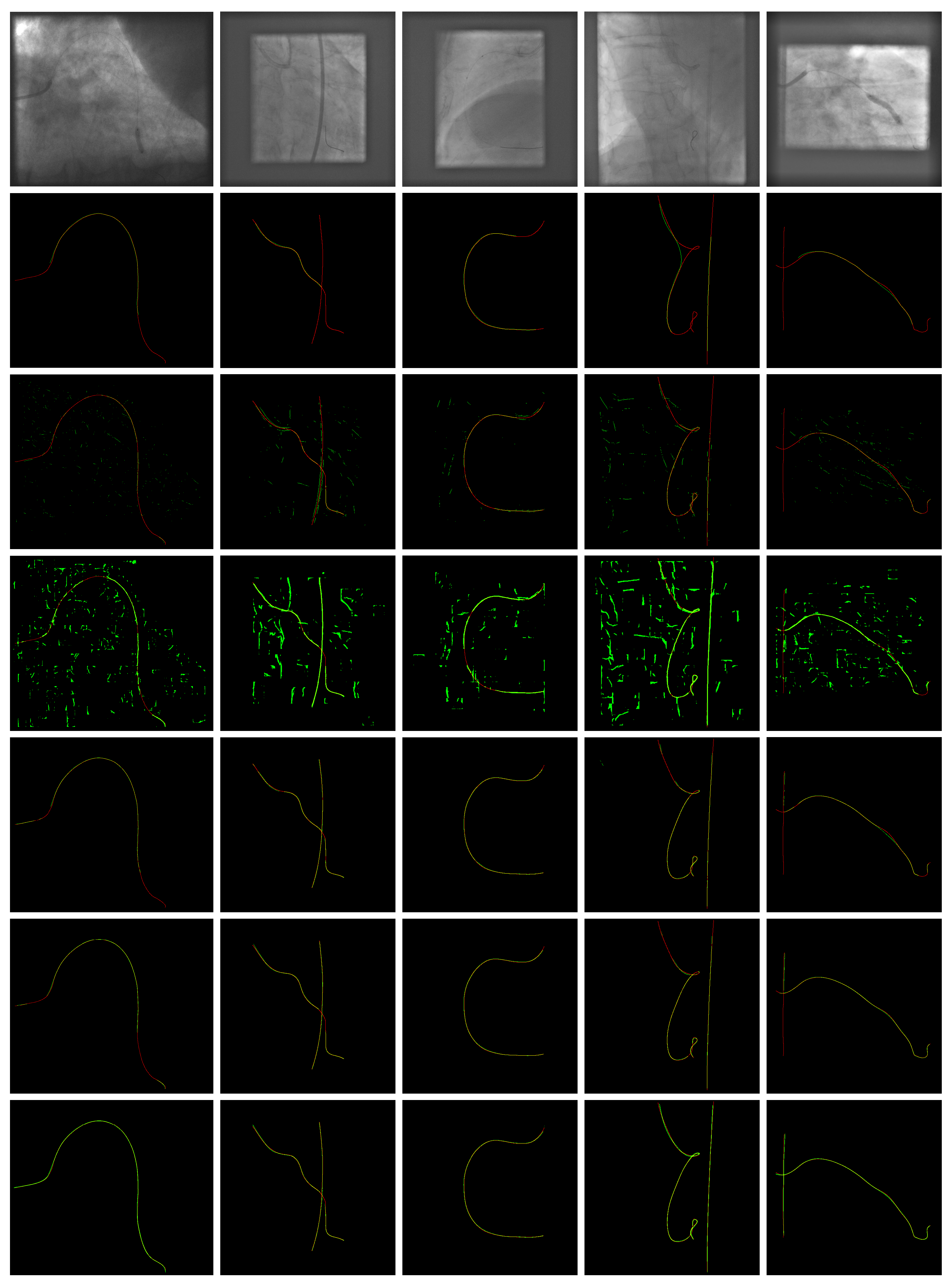
Figure A2.
Example segmentation results (green) and annotation (red) on the CathAction test set. From top to bottom: input images, Hierarchical [18], SCNN[8], Two-Phase[10], Res-UNet[2], nnU-Net[3] and MSLNet-Lor.
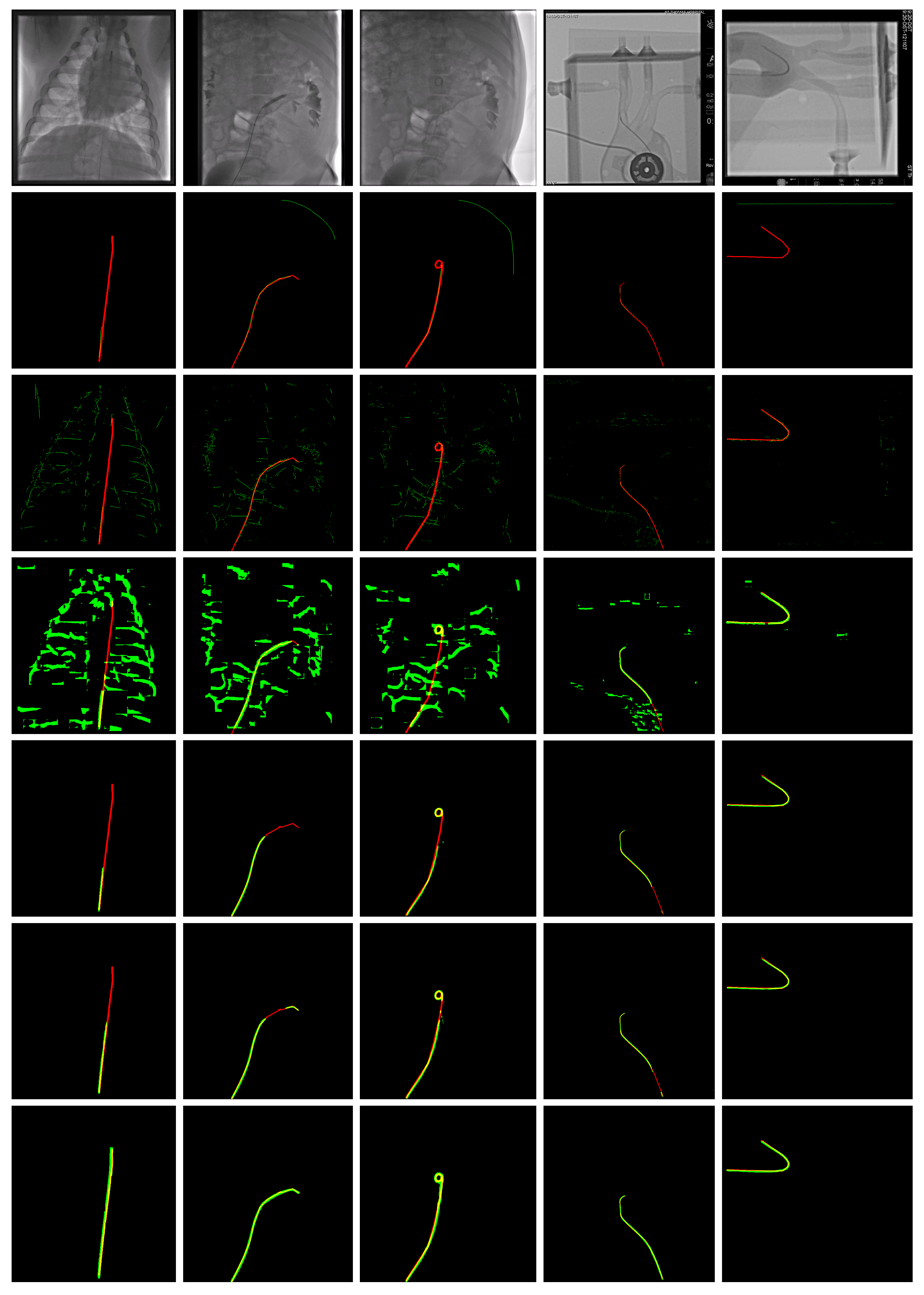
Figure A3.
Example localization results (green) and annotation (red) on the guidewire test set.
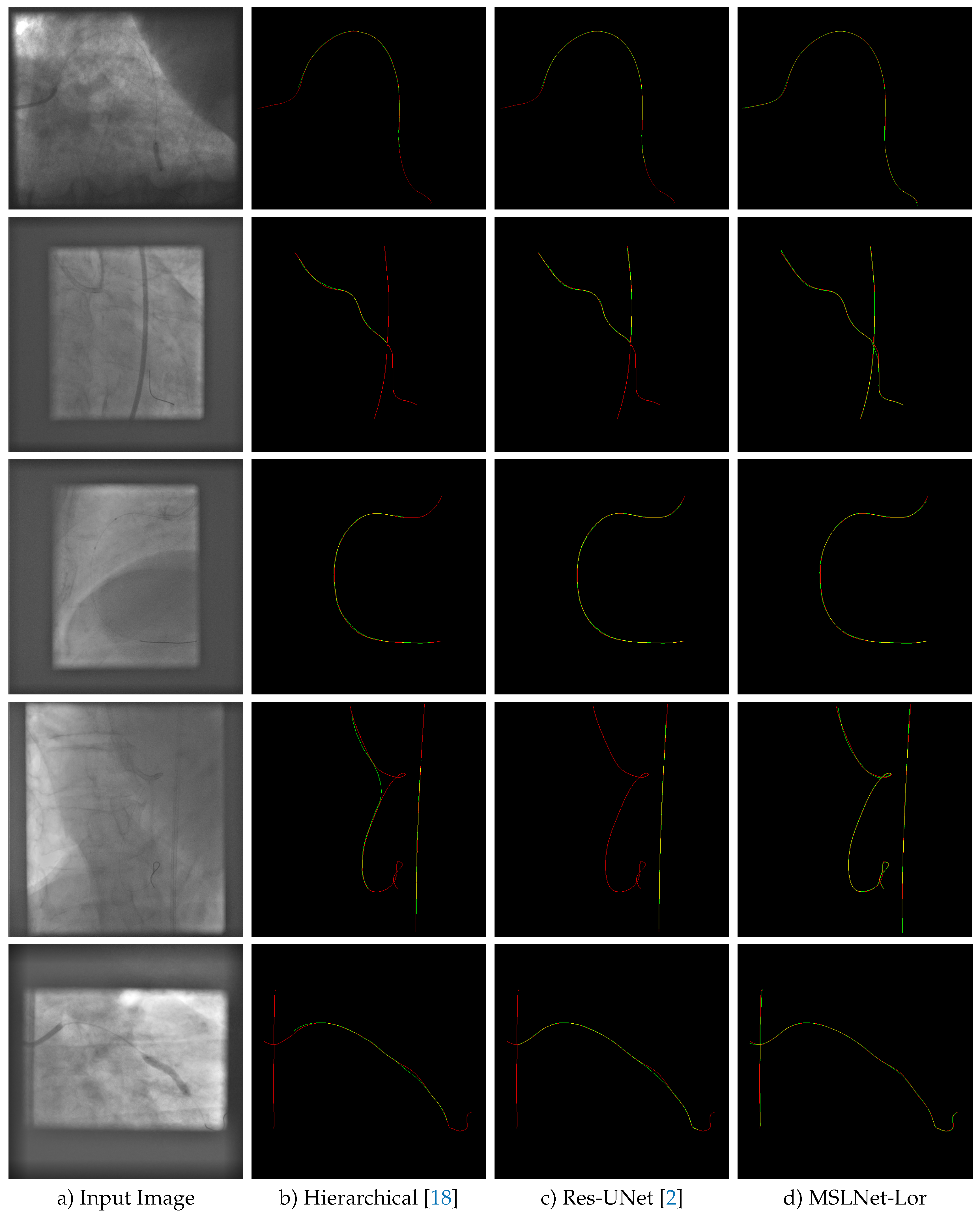
| a) Input Image | b) Hierarchical [18] | c) Res-UNet [2] | d) MSLNet-Lor |
Figure A4.
Example localization results (green) and annotation (red) on the CathAction test set. The annotation was thinned, as mentioned in Section 4.2.
Figure A4.
Example localization results (green) and annotation (red) on the CathAction test set. The annotation was thinned, as mentioned in Section 4.2.
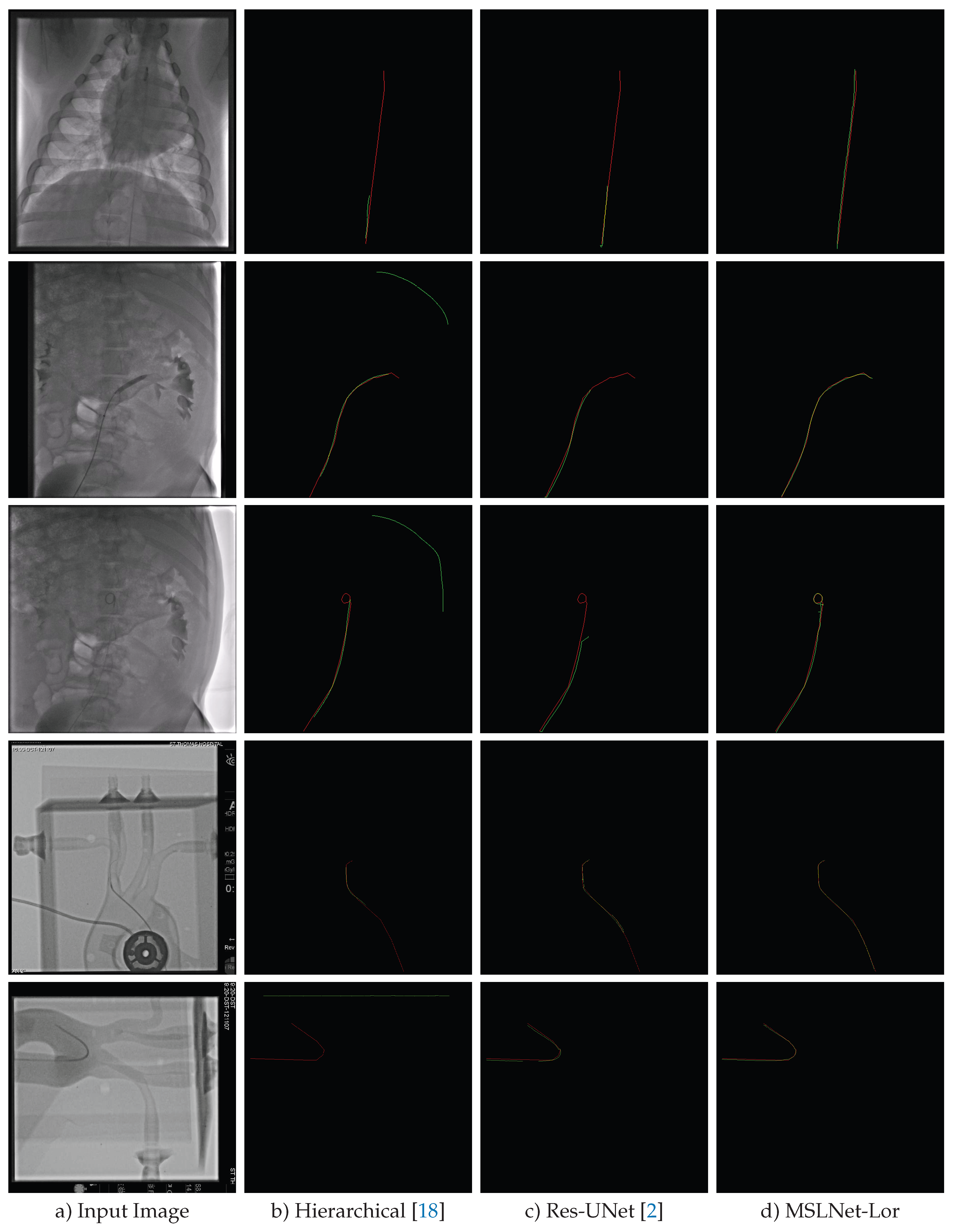
| a) Input Image | b) Hierarchical [18] | c) Res-UNet [2] | d) MSLNet-Lor |
References
- Murphy, S.L.; Kochanek, K.D.; Xu, J.; Arias, E. Mortality in the United States, 2023. NCHS Data Brief 2024, p. CS356116.
- Ambrosini, P.; Ruijters, D.; Niessen, W.J.; Moelker, A.; van Walsum, T. Fully automatic and real-time catheter segmentation in X-ray fluoroscopy. In Proceedings of the Medical Image Computing and Computer-Assisted Intervention- MICCAI 2017: 20th International Conference, Quebec City, QC, Canada, September 11-13, 2017, Proceedings, Part II 20. Springer, 2017, pp. 577–585.
- Isensee, F.; Jaeger, P.F.; Kohl, S.A.; Petersen, J.; Maier-Hein, K.H. nnU-Net: a self-configuring method for deep learning-based biomedical image segmentation. Nature methods 2021, 18, 203–211. [Google Scholar] [CrossRef] [PubMed]
- Ronneberger, O.; Fischer, P.; Brox, T. U-net: Convolutional networks for biomedical image segmentation. In Proceedings of the MICCAI; 2015; pp. 234–241. [Google Scholar]
- He, K.; Zhang, X.; Ren, S.; Sun, J. Deep residual learning for image recognition. In Proceedings of the Proceedings of the IEEE conference on computer vision and pattern recognition, 2016, pp.
- Ma, Y.; Alhrishy, M.; Panayiotou, M.; Narayan, S.A.; Fazili, A.; Mountney, P.; Rhode, K.S. Real-time guiding catheter and guidewire detection for congenital cardiovascular interventions. In Proceedings of the International Conference on Functional Imaging and Modeling of the Heart. Springer; 2017; pp. 172–182. [Google Scholar]
- Frangi, A.F.; Niessen, W.J.; Vincken, K.L.; Viergever, M.A. Multiscale vessel enhancement filtering. In Proceedings of the International conference on medical image computing and computer-assisted intervention. Springer, 1998, pp. 130–137.
- Li, D.; Barbu, A. Training a Steerable CNN for Guidewire Detection. In Proceedings of the CVPR; 2020; pp. 13955–13963. [Google Scholar]
- Gherardini, M.; Mazomenos, E.; Menciassi, A.; Stoyanov, D. Catheter segmentation in X-ray fluoroscopy using synthetic data and transfer learning with light U-nets. Computer Methods and Programs in Biomedicine 2020, 192, 105420. [Google Scholar] [CrossRef] [PubMed]
- Chen, K.; Qin, W.; Xie, Y.; Zhou, S. Towards real time guide wire shape extraction in fluoroscopic sequences: a two phase deep learning scheme to extract sparse curvilinear structures. Computerized Medical Imaging and Graphics 2021, 94, 101989. [Google Scholar] [CrossRef] [PubMed]
- Zhang, G.; Wong, H.C.; Wang, C.; Zhu, J.; Lu, L.; Teng, G. A temporary transformer network for guide-wire segmentation. In Proceedings of the International Congress on Image and Signal Processing, BioMedical Engineering and Informatics. IEEE; 2021; pp. 1–5. [Google Scholar]
- Zhang, G.; Wong, H.C.; Zhu, J.; An, T.; Wang, C. Jigsaw training-based background reverse attention transformer network for guidewire segmentation. Int. Journal of Computer Assisted Radiology and Surgery 2023, 18, 653–661. [Google Scholar] [CrossRef] [PubMed]
- Kongtongvattana, C.; Huang, B.; Kang, J.; Nguyen, H.; Olufemi, O.; Nguyen, A. Shape-sensitive loss for catheter and guidewire segmentation. In Proceedings of the International Conf. on Robot Intelligence Technology and Applications; 2023; pp. 95–107. [Google Scholar]
- Chen, J.; Lu, Y.; Yu, Q.; Luo, X.; Adeli, E.; Wang, Y.; Lu, L.; Yuille, A.L.; Zhou, Y. Transunet: Transformers make strong encoders for medical image segmentation. arXiv preprint arXiv:2102.04306 2021.
- Cao, H.; Wang, Y.; Chen, J.; Jiang, D.; Zhang, X.; Tian, Q.; Wang, M. Swin-unet: Unet-like pure transformer for medical image segmentation. In Proceedings of the ECCV; 2022; pp. 205–218. [Google Scholar]
- Isensee, F.; Wald, T.; Ulrich, C.; Baumgartner, M.; Roy, S.; Maier-Hein, K.; Jaeger, P.F. nnu-net revisited: A call for rigorous validation in 3d medical image segmentation. In Proceedings of the MICCAI; 2024; pp. 488–498. [Google Scholar]
- Huang, B.; Vo, T.; Kongtongvattana, C.; Dagnino, G.; Kundrat, D.; Chi, W.; Abdelaziz, M.; Kwok, T.; Jianu, T.; Do, T.; et al. Cathaction: A benchmark for endovascular intervention understanding. arXiv preprint arXiv:2408.13126 2024.
- Barbu, A.; Athitsos, V.; Georgescu, B.; Boehm, S.; Durlak, P.; Comaniciu, D. Hierarchical learning of curves application to guidewire localization in fluoroscopy. In Proceedings of the CVPR, 2007, pp. 1–8.
- Zheng, Y.; Barbu, A.; Georgescu, B.; Scheuering, M.; Comaniciu, D. Four-chamber heart modeling and automatic segmentation for 3-D cardiac CT volumes using marginal space learning and steerable features. IEEE transactions on medical imaging 2008, 27, 1668–1681. [Google Scholar] [CrossRef] [PubMed]
- Barbu, A.; She, Y.; Ding, L.; Gramajo, G. Feature selection with annealing for computer vision and big data learning. IEEE transactions on pattern analysis and machine intelligence 2016, 39, 272–286. [Google Scholar] [CrossRef] [PubMed]
- Lam, L.; Lee, S.W.; Suen, C.Y. Thinning methodologies-a comprehensive survey. IEEE Transactions on Pattern Analysis & Machine Intelligence 1992, 14, 869–885. [Google Scholar]
- Crouse, D.F. On implementing 2D rectangular assignment algorithms. IEEE Transactions on Aerospace and Electronic Systems 2016, 52, 1679–1696. [Google Scholar] [CrossRef]
- Marchant, R.; Jackway, P. Feature detection from the maximal response to a spherical quadrature filter set. In Proceedings of the 2012 International Conference on Digital Image Computing Techniques and Applications (DICTA). IEEE; 2012; pp. 1–8. [Google Scholar]
Disclaimer/Publisher’s Note: The statements, opinions and data contained in all publications are solely those of the individual author(s) and contributor(s) and not of MDPI and/or the editor(s). MDPI and/or the editor(s) disclaim responsibility for any injury to people or property resulting from any ideas, methods, instructions or products referred to in the content. |
© 2025 by the authors. Licensee MDPI, Basel, Switzerland. This article is an open access article distributed under the terms and conditions of the Creative Commons Attribution (CC BY) license (http://creativecommons.org/licenses/by/4.0/).
Copyright: This open access article is published under a Creative Commons CC BY 4.0 license, which permit the free download, distribution, and reuse, provided that the author and preprint are cited in any reuse.


