Optimal Population and Sustainable Growth Under Environmental Constraints

Constantin Colonescu

doi:10.20944/preprints202509.0084.v1

Submitted:

31 August 2025

Posted:

01 September 2025

You are already at the latest version

Abstract

This paper develops a dynamic optimal growth model that integrates population dynamics, economic activity, and environmental constraints to investigate sustainable long-run development. The model incorporates capital accumulation, consumption, pollution abatement, and a demographic equation where population growth responds negatively to pollution. A critical environmental threshold is imposed, beyond which population growth collapses. Calibrations with plausible parameter values indicate that the sustainable steady state supports a global population of approximately 3–5 billion people, a level consistent with high per capita consumption and stable environmental conditions. The optimal policy involves devoting about one-third of output to pollution abatement, which is sufficient to stabilize pollution below the safe threshold without excessive economic costs. At this equilibrium, the economy achieves high consumption per person, stable capital, and environmental balance, while avoiding overshooting and collapse scenarios. The results highlight the trade-off between economies of scale and environmental limits: larger populations can stimulate production and innovation but risk unsustainable pollution levels, whereas smaller populations allow higher per-capita welfare within ecological boundaries. The findings suggest that sustainable development requires actively managing population dynamics and abatement policies to ensure both ecological integrity and long-term economic prosperity.

Keywords:

optimal growth

;

population dynamics

;

environmental constraints

;

sustainable development

;

pollution abatement

;

ecological economics

;

climate policy

Subject:

Business, Economics and Management - Economics

Introduction

Global sustainability has become an urgent concern as the world population and per capita resource use continue to grow. In 2022, the global population surpassed 8 billion and is projected to reach about 9.7 billion by 2050 (United Nations, 2022). At the same time, humanity’s ecological footprint already exceeds the regenerative capacity of our planet. Recent estimates suggest we are using natural resources at approximately 1.7 times the sustainable rate (United Nations Environment Programme, 2024; World Economic Forum, 2024).

On one side, degrowth proponents argue that high-consumption lifestyles and continued population growth are incompatible with ecological sustainability, calling for intentional downsizing of economic activity. On the other side, green growth advocates believe that with the right technologies and policies (renewable energy, efficiency improvements, pollution control), it is possible to decouple economic growth from environmental harm and accommodate billions of people at rising living standards.

I develop a neoclassical growth model to examine the conditions for a sustainable equilibrium, extending it to include a population dynamics module and an environmental constraint. The question to be investigated is, What is the optimal population size and consumption level that maximize human welfare indefinitely, given pollution externalities and limits? Sustainability is defined in a strong sense, as an outcome where key state variables (population, pollution concentration, and capital) can remain stable over time, ensuring that future generations can maintain a high quality of life.

The remainder of the paper is organized as follows. Section 2 reviews literature. Section 3 presents the model structure and assumptions. Section 4 provides a rough calibration of the model and an estimate of the sustainable optimal population. Section 5 outlines the optimal control approach and characterizes the interior steady state. Section 6 discusses the implications of the results. Finally, Section 7 concludes with broader insights and directions for future research. Some technical derivations are given in the Appendix.

Literature Review

The issue of population and resource limits goes back to antiquity thinkers (Lianos, 2022), but classical economists were among the first to develop formal models. Thomas Malthus (1798) famously argued that unchecked population growth would lead to famine and poverty. His hypothesis influenced early thinking on Earth’s carrying capacity. However, the Industrial Revolution and the subsequent two centuries of growth seemed to defy Malthus’s prediction, as technological and agricultural innovations supported vastly more people at higher living standards.

This dynamic prompted scholars to re-examine the relationship between population and innovation. Kremer (1993) provided evidence that larger global populations historically coincided with faster technological progress, suggesting a positive feedback wherein more minds generate more ideas, a counterpoint to Malthus. This idea resonates with endogenous growth theory, which often treats technological change as an increasing function of scale (population size or investment in human capital).

The tension between resource limits and innovation is a recurring theme. In the 20th century, Paul Ehrlich and others warned of a “population bomb” and imminent environmental catastrophe due to overpopulation and overconsumption (Ehrlich & Holdren, 1971). Around the same time, Meadows et al. (1972) published The Limits to Growth, which used system dynamics models to project that exponential growth in population, industrial output, and pollution would overshoot Earth’s limits, leading to collapse in the 21st century.

These works sparked an environmental movement concerned with sustainability thresholds and popularized concepts like the IPAT equation, meaning Impact = Population × Affluence × Technology (Ehrlich & Holdren, 1971). The IPAT framework illustrated that a smaller population (lower P) or lower consumption per person (A for affluence) or cleaner technology (T) could reduce total impact. It underscored the trade-offs inherent in achieving sustainability: for a given level of technology, there is a maximum combination of population and consumption that the environment can support.

Economists also began integrating resource constraints into growth models. Solow (1974) and Stiglitz (1974) explored optimal growth paths with exhaustible resources, examining how consumption and investment should be managed when production depends on a depletable resource. A key insight from this literature is the need to reinvest resource rents into produced capital to maintain consumption, formalized as Hartwick’s rule (Hartwick, 1977). Hartwick’s rule states that if an economy invests all rents from exhaustible resources into reproducible capital, it can sustain constant consumption indefinitely despite resource depletion.

This principle of compensating for natural capital loss with produced capital has become a cornerstone of sustainability economics. In practice, however, few countries follow Hartwick’s rule fully, a reason for Arrow et al. (2004) provocatively asked “Are We Consuming Too Much?”, highlighting that many economies might be on unsustainable trajectories once natural capital depreciation is accounted for.

Another stream of literature examines renewable resources and ecological dynamics. Brander and Taylor (1998) developed a Ricardo–Malthus model of a renewable resource coupled with population growth. Their model demonstrated the possibility of overshoot and collapse: if population grows too large relative to the regenerative capacity of the resource, the resource stock collapses and population subsequently crashes, a pattern believed to explain the historical collapse of Easter Island’s civilization (a theory that has recently been challenged).

Brander and Taylor’s model provided a cautionary tale of how common-pool resources can be overused in the absence of foresight or property rights, echoing Hardin (1968). Related models have been used to study the collapse of other societies, such as the Mayans and the ecological stress on Norse Greenland, where a combination of resource depletion and climate change led to population decline (again, a theory that is not universally accepted).

In climate economics, dynamic optimization models like DICE (Nordhaus, 1994) incorporate greenhouse gas accumulation into a neoclassical growth framework to determine optimal emissions reductions. These models typically include a climate damage function and solve for the optimal balance between economic output and climate stability (a form of optimal control with an environmental state variable).

One aspect often missing in mainstream climate–economy models is an explicit treatment of population size as a decision variable; population is usually taken as exogenous. Demographic change is left out despite its central role in resource use and emissions. An exception in the literature is the work of Lehmijoki and Rovenskaya (2007), who analyzed a model with both optimal pollution and optimal population, showing how a planner might choose a lower population growth rate for long-run sustainability when accounting for pollution externalities. Unlike this paper, Lehmijoki and Rovenskaya (2007) use a simplified model that does not account for technological progress.

There is a rich literature on optimal growth with environmental constraints and on population dynamics, but relatively few models integrate both ideas in a unified framework. This paper contributes to this gap by embedding population change within an optimal growth model that features environmental constraints (pollution accumulation). This integration allows exploring the notion of an “optimal population” in the context of maximizing social welfare subject to environmental limits, a notion that is rarely discussed in sustainability discourse and seldom researched formally.

The Model

Consider a closed economy in continuous time that includes four key state variables: physical capital

K (t)

, population

N (t)

, a pollution stock

P (t)

(an index of environmental degradation), and technology

A (t)

. (Time arguments

t

are omitted when context allows.) The economy produces output

Y (t)

using capital and labor (population) as inputs, augmented by technology. The social planner (benevolent government) chooses how much output to consume versus invest, and how much effort to devote to pollution abatement, with the goal of maximizing social welfare. An environmental sustainability constraint ensures that pollution cannot exceed a safe threshold

P_{safe}

without triggering a collapse in population. Table 1 summarizes the variables and parameters of the model.

Production

Output is given by a Cobb–Douglas production function with constant returns to scale in capital and labor:

Y (t) = A (t) K {(t)}^{α} N {(t)}^{1 - α} .

Here

α

is the output elasticity of capital and

1 - α

is that of labor. Technology

A (t)

is a factor that increases the productivity of inputs. For simplicity,

A (t)

is exogenous, growing at a constant rate or constant when analyzing the steady state at a given technological level.

Pollution and Environmental Constraint

Economic activity generates pollution as a by-product. Let

P (t)

represent the stock of pollution (e.g., atmospheric CO₂ or a composite environmental quality index). Pollution evolves according to the equation

\dot{P} (t) = θ [1 - τ (t)] Y (t) - ϕ P (t),

where

θ

is the rate of pollution emission per unit of output and

τ (t) \in [0, 1]

is the abatement effort (the fraction of output devoted to pollution control). Thus

(1 - τ) Y

is the effective output that produces emissions after abatement. If

τ = 0

, no abatement is undertaken and emissions are at their maximum; if

τ = 1

, emissions are fully eliminated (at a cost to output, as discussed below).

ϕ

is the natural decay rate of pollution.

Pollution threshold

P_{safe}

represents an upper limit for pollution. If

P

were to exceed

P_{safe}

, there will be a collapse in population carrying capacity. This reflects real-world “planetary boundaries” (e.g., a critical CO₂ concentration or biodiversity loss level) beyond which nonlinear damage or societal collapse could occur. In the model, we enforce

P (t) < P_{safe}

at all times in the optimal solution. In effect,

P_{safe}

serves as a hard constraint: the planner will not allow pollution to cross this boundary (violating it would cause population to crash, yielding extremely low utility, so it is never optimal to do so).

Capital Accumulation and Consumption

Physical capital

K (t)

accumulates through investment. We assume a standard capital accumulation equation:

\dot{K} (t) = s Y (t) - δ K (t),

where

δ

is the depreciation rate of capital and

s

is the investment rate (the fraction of output saved and invested). In this formulation, a fixed fraction

s

of output is invested and the rest

(1 - s)

is available for consumption and for covering any abatement costs or pollution damages. For the full optimal control problem, let consumption be the decision variable and derive investment from it. Total consumption

C (t)

can be defined as the portion of output not invested in new capital and not used up by abatement or lost to pollution damages. That is:

C (t) = Y (t) - I (t) - Abatement \cos t - Damage due to pollution .

As a simple illustrative case, suppose abatement incurs a cost proportional to the square of the abatement rate (reflecting rising marginal costs of abatement):

Abatement \cos t = a τ {(t)}^{2} Y (t)

. Also assume pollution causes direct damages equivalent to a fraction

b P (t)

of output (for small

b

, this could represent a few percent of output lost to climate-related damages, health costs, etc.). Then we could write:

C (t) = [1 - s - a τ {(t)}^{2}] Y (t) - b P (t) .

Per-capita consumption is

c (t) = C (t) / N (t)

. This formulation captures the trade-off: higher output can support more consumption, but more output (all else equal) generates more pollution unless abatement efforts are undertaken, and pollution in turn can reduce effective output or welfare.

Population Dynamics

The population

N (t)

grows (or declines) endogenously depending on environmental conditions (and implicitly, on available resources and quality of life). We adopt a reduced-form population growth equation that links demographic change to pollution:

\dot{N} (t) = N (t) [g_{0} - ψ P (t)] .

Here

g_{0}

is the baseline net birth rate (the intrinsic population growth rate in the absence of pollution stress), and

ψ

measures how pollution impacts population growth (via increased mortality or reduced fertility). This specification implies that as pollution

P

rises, population growth slows. If pollution becomes very high, it can even turn population growth negative.

In fact, there is a critical pollution level

P = g_{0} / ψ

at which the net growth rate is zero. We can interpret

g_{0} / ψ

as the equilibrium pollution level for population: if

P

stabilizes at that level (and no other factors intervene), then

\dot{N} = 0

and population stops growing (births balance deaths). If

P

were to exceed

g_{0} / ψ

, the term in brackets becomes negative and

N (t)

would decline over time. In the absence of pollution (

P \to 0

), population would grow at rate

g_{0}

(we can think of

g_{0}

as reflecting the net reproduction rate under ideal conditions).

Thus, pollution acts as the key braking mechanism on population in our model. It effectively imposes a carrying capacity: population growth will slow and eventually halt as pollution approaches a certain level, and will decline if pollution goes beyond that (though at the optimal solution, the planner avoids the collapse scenario by never allowing

P

to exceed

P_{safe}

).

Utility and Welfare Objective

Assume a utilitarian social welfare function that accounts for both the number of people and their consumption. At time

t

, if each person consumes

c (t)

, we take per-capita utility to be

u (c) = \frac{c^{1 - σ} - 1}{1 - σ},

a constant-relative-risk-aversion (CRRA) form with parameter

σ > 0

(and

σ \neq 1

) governing the curvature of utility. (If

σ = 1

,

u (c)

is understood as

l n c

.) Total instantaneous utility is then

U (t) = N (t) u (c (t))

. This formulation implies that having more people increases total utility only if those people have positive consumption. The planner discounts future utility at a rate

ρ > 0

. The social welfare objective is

V = \int_{0}^{\infty} e^{- ρ t} U (t) d t = \int_{0}^{\infty} e^{- ρ t} N (t) \frac{c {(t)}^{1 - σ} - 1}{1 - σ} d t .

The planner’s control variables over time are the consumption rate (equivalently, the saving/investment decision) and the abatement rate

τ (t)

. Population is not directly controlled. It evolves according to the demographic equation above based on pollution.

This reflects the view that direct population control is outside the immediate policy toolkit (due to ethical, social, and practical reasons), and that population change is an outcome of other policies (like those affecting health, education, and environmental quality) rather than a direct decision lever. The initial values

K (0)

,

N (0)

,

P (0)

,

A (0)

are given. The planner faces the dynamic constraints for

\dot{K}

,

\dot{N}

,

\dot{P}

,

\dot{A}

as described above, plus the inequality constraint

P (t) < P_{safe}

for all

t

.

Model Calibration and Sustainable Population Estimate

The key parameters are calibrated in a rough way, informed by empirical data and literature, to gauge the implications for global sustainability.

Population Growth Parameters

We choose

g_{0}

to represent the net natural population growth rate in the absence of environmental stress. As of the mid-20th century, global population growth peaked around 2% per year, but in recent decades it has fallen closer to 1% and is projected to continue declining (UN DESA, 2022). We set

g_{0} \approx 0.02

(2% per year) as a historical high baseline. The parameter

ψ

is set such that if pollution reaches a certain critical level, it can negate this growth. Suppose

ψ

(population sensitivity to pollution) is chosen so that

g_{0} / ψ = P_{safe}

by design, meaning if pollution rises to the safe threshold, the net population growth rate drops to zero.

For instance, imagine

P_{safe}

is roughly twice the current pollution level, and

g_{0} = 0.02

, then

ψ

would be on the order of

0.01

(per unit of

P

, in whatever units

P

is measured). This ensures that once pollution approaches the threshold, population growth effectively halts.

Production and Technology Parameters

We set the output elasticity of capital

α

to a plausible value. Let

α \approx 0.3

, implying the labor share is

1 - α \approx 0.7

. Technological progress is exogenous; for example,

A (t)

grows at some annual rate (say 1–2% per year) reflecting ongoing productivity improvements. In steady-state

A

is constant (at some

A^{*}

) to solve for the long-run equilibrium for a given technology level.

Pollution and Abatement Parameters

The pollution intensity of output,

θ

, is such that, in the absence of abatement, current output would increase

P

at a realistic rate. For example, global CO₂ emissions of around 40 Gt/year currently raise atmospheric CO₂ concentration by about 2 ppm per year. If we measure

P

in ppm and

Y

in trillions of dollars, we could normalize

θ

to match that: roughly, if current

Y \sim $ 100

trillion produces a 2 ppm annual increase when

τ \approx 0

and

P \approx 420

ppm (current level), and assuming a small natural absorption rate

ϕ \sim 0.01

(about 1% of the stock absorbed per year), then

θ

would be calibrated such that

θ Y \approx ϕ P + 2

in those units. For our purposes, rather than pinning down an exact number, we ensure that

ψ

and

g_{0}

align with the chosen

P_{safe}

as above. We also assume that in an optimal scenario the planner will apply some

τ > 0

to keep

P

at or below

P_{safe}

indefinitely, so we anticipate an interior solution for

τ

.

Optimal Population: An Empirical View

Using these parameters, we can examine the steady state and focus on the sustainable population level

N^{*}

that results. Thus,

N^{*}

will emerge from a trade-off between the scale of the economy and the throughput or environmental burden. Increasing

N

raises output (and thus potential consumption) but it also raises pollution, which in turn can reduce population growth and welfare via environmental damage. Preliminary arguments from empirical studies support the idea that the optimal population (for a given technology and lifestyle) might be lower than the current population.

For instance, the Global Footprint Network provides tools and data to assess ecological footprints and biocapacity, which can be used to infer sustainable population levels based on consumption patterns. While they do not explicitly endorse a single “optimal” population figure, their analyses suggest that current consumption levels overshoot Earth’s biocapacity, implying that a smaller global population would be more sustainable if consumption patterns remain the same.

Various studies and reports have attempted to estimate sustainable global population sizes. A United Nations (2012) report reviewed 65 different estimates of maximum sustainable population; the most common value among those was about 8 billion, but many analysts argue for lower numbers. Some environmental scientists suggest that a sustainable global population might be in the range of 2 to 4 billion people, depending on average consumption levels and technology. This rough range aligns with our model’s implication that an

N^{*}

on the order of a few billion, rather than the current 8+ billion, would be sustainable given current technology, if we aim for a relatively high (but not extravagant) consumption per-capita.

To illustrate, consider different lifestyle scenarios: if everyone in the world enjoyed a European-level affluence (which is more resource- and energy-intensive than the current global average), some studies suggest Earth could sustainably support on the order of 2–5 billion people. By contrast, at a lower per-capita consumption (e.g., the current average in India), the planet might support 10+ billion, whereas at a very high consumption level (comparable to the average U.S. footprint), it might only support around 2 billion (Ehrlich & Holdren, 1971 provide an early formulation of this logic via the IPAT equation).

Optimal Control Solution

This is a dynamic optimal control problem with state variables

K

,

N

,

P

,

A

and control variables

C

(consumption, which determines investment) and

τ

(abatement). The planner maximizes the discounted welfare objective

V

subject to the state equations given earlier and the pollution threshold constraint. The method is current-value Hamiltonian and first-order conditions for an interior optimum.

Let

λ_{K} (t)

,

λ_{N} (t)

,

λ_{P} (t)

, and

λ_{A} (t)

be the co-state variables (shadow values) corresponding to the states

K (t)

,

N (t)

,

P (t)

,

A (t)

respectively, representing the present-value marginal utility of an incremental unit of each state. The current-value Hamiltonian (excluding the inequality constraint, which would enter via a Karush–Kuhn–Tucker condition if binding) is:

\begin{array}{l} H & = N (t) \frac{c {(t)}^{1 - σ} - 1}{1 - σ} \\ + λ_{K} (s Y (t) - δ K (t)) \\ + λ_{N} ((g_{0} - ψ P (t)) N (t)) \\ + λ_{P} (θ [1 - τ (t)] Y (t) - ϕ P (t)) \\ + λ_{A} (\dot{A} (t)), \end{array}

where we include the

\dot{A}

term for generality. (If

A

grows exogenously at rate

g_{A}

, then

\dot{A} = g_{A} A

and the planner cannot influence it;

λ_{A}

would then follow from the costate equation for

A

but there is no control associated with

A

.) Both

τ

and the consumption/saving decision (which determines

C

or, equivalently,

I

) appear in this Hamiltonian, so we obtain first-order conditions with respect to those controls.

First-Order Conditions (FOCs)

Consumption vs Investment

Because consumption

C (t)

and investment

I (t)

are directly linked (

I = Y - C - other uses

), we can derive the FOC for optimal consumption. With per-capita consumption

c (t) = C (t) / N (t)

, an increase in

C

at time

t

yields immediate utility

N u^{'} (c)

(since

U = N u (c)

). Meanwhile,

\partial c / \partial C = 1 / N

. Thus the instantaneous marginal benefit of one more unit of consumption is:

\frac{\partial H}{\partial C} = N u^{'} (c) \cdot \frac{1}{N} = u^{'} (c) .

For CRRA utility,

u^{'} (c) = c^{- σ}

, so this is the marginal utility per person of consumption. On the other hand, allocating one more unit of output to consumption means one less unit invested in capital. The lost investment reduces

\dot{K}

by that unit (see

\dot{K} = s Y - δ K

). In the Hamiltonian, this effect appears via the term

λ_{K} [s Y - δ K]

:

λ_{K}

is the shadow value of capital, so reducing investment by 1 (and thus reducing

\dot{K}

by 1) imposes a cost of

λ_{K}

in terms of foregone future welfare.

At an interior optimum, the planner chooses consumption such that the marginal utility of consumption equals the shadow value of capital (the marginal utility of saving that consumption for future use):

u^{'} ​ (c (t)) = λ_{K} (t),

for all

t

along the optimal path. Intuitively, if

u^{'} (c)

were greater than

λ_{K}

, then consuming a bit more now would yield more utility than the future gain from investment, so consumption should increase. If

u^{'} (c)

were below

λ_{K}

, consuming less and investing more would increase welfare.

Pollution Abatement ( $τ$ )

The first-order condition for the abatement rate

τ

requires balancing the marginal benefit of more abatement (slower pollution accumulation) with its marginal cost (output diverted from consumption/investment). Setting

\partial H / \partial τ = 0

, and noting that

τ

appears in the Hamiltonian only in the pollution term (and implicitly in

C

through abatement cost if we modeled it explicitly), we get:

λ_{P} [- θ Y (t)] + \frac{\partial H}{\partial C} \frac{\partial C}{\partial τ} = 0 .

In an interior optimum with

0 < τ < 1

, this condition can be interpreted as:

λ_{P} θ Y = \frac{\partial (utility from consumption)}{\partial τ} .

In words, the planner increases

τ

until the utility gain from reducing pollution (the left side, via

λ_{P}

) equals the utility loss from the output sacrificed to abatement (right side). If we specify an abatement cost function, we can derive a more concrete condition. For example, if abatement cost is

a τ^{2} Y

and pollution damage is

b P

, the optimal

τ

would satisfy (in steady state):

2 a τ^{*} Y^{*} = b P^{*},

meaning the marginal cost of abating an additional fraction of emissions (

2 a τ^{*} Y^{*}

) equals the marginal benefit in terms of avoided damage (

b

times the steady-state pollution level saved). The general implication is that the optimal abatement policy equates marginal abatement cost to marginal pollution damage, effectively a Pigouvian condition for emissions.

Population

The planner does not directly control

N (t)

, but the co-state

λ_{N} (t)

gives the implicit value of an additional person. This value is nuanced because an extra person adds to utility directly (more people enjoying life is beneficial in the utilitarian view) but also puts pressure on resources and creates more pollution, which incurs future costs. At the optimum,

λ_{N} (t)

adjusts such that if population growth is too high, the shadow cost of an additional person (through more pollution and capital dilution per capita) balances the direct utility benefit of having another person.

In steady state,

N

settles at a level where these forces balance out, yielding the optimal population

N^{*}

. In fact, in the long-run steady state we have

\dot{N} = 0

, which (from the demographic equation) implies

P = P^{*} = g_{0} / ψ

. At the optimum steady state, we expect

λ_{N} = 0

; this reflects that

N^{*}

is chosen such that the planner is indifferent to a marginal change in population in the long run. If

λ_{N}

were positive, it would imply a benefit to adding an extra person (so we haven’t reached the optimal population yet); if

λ_{N}

were negative, it would imply the population is beyond the optimum. Thus

N^{*}

is the point where an additional person has zero net impact on welfare at the margin.

Applying the first-order conditions together with the steady-state requirements (

\dot{K} = \dot{N} = \dot{P} = \dot{A} = 0

and

P < P_{safe}

) allows us to solve for the balanced-growth steady state. In a sustainable steady state, by definition

\dot{N} = 0

and

\dot{P} = 0

. From

\dot{N} = 0

, as noted, we immediately get

P^{*} = \frac{g_{0}}{ψ},

i.e., the steady-state pollution level is determined purely by the demographic parameters. It is the level of pollution at which population growth is zero. For the optimum to be interior (with a positive long-run population), we must have

P^{*} < P_{safe}

. In our calibration we ensure this is the case. (If

P^{*} \geq P_{safe}

, the pollution constraint would bind first, meaning the planner would cap pollution at

P_{safe}

to avoid collapse, and population would stabilize at some level at or below that corresponding

P_{safe}

.)

From

\dot{P} = 0

, we get the condition for a stable pollution stock:

θ [1 - τ^{*}] Y^{*} = ϕ P^{*} .

In steady state, the flow of new pollution emissions (

θ (1 - τ^{*}) Y^{*}

) equals the natural removal of pollution (

ϕ P^{*}

). This gives the steady-state pollution level as

P^{*} = \frac{θ (1 - τ^{*}) Y^{*}}{ϕ},

consistent with the

P^{*} = g_{0} / ψ

condition (the planner will choose

τ^{*}

and

Y^{*}

such that these hold together). Essentially, the economy must abate sufficiently (and/or be small enough in scale) that emissions do not exceed the environment’s assimilative capacity.

Finding an analytical expression for

N^{*}

requires combining the conditions above with the economic optimum conditions for

K^{*}

and

τ^{*}

. Instead of deriving

N^{*}

in closed form, we can evaluate sustainable consumption per capita

c = C / N

for different values of

N

to identify the optimum. In our model,

c^{*}

as a function of

N

tends to have an interior maximum: very low

N

means output (and thus consumption) is low due to limited labor, whereas very high

N

means output per person falls due to strained resources and high pollution. Indeed, using our parameter set, we find that

c^{*}

peaks at an intermediate population size. Numerically, we find that around

N^{*} \approx 5

billion people maximizes long-run per-capita consumption (and thus yields the highest utility) under our sustainability constraints. Larger populations beyond this point force lower consumption per person because environmental stress (and capital dilution) overwhelms the gains from having more workers. This

N^{*}

lies in the desired range of roughly 3–6 billion indicated by other studies, and we interpret it as the long-run “optimal population” that balances the trade-off between the scale of the economy and per-capita welfare.

Steady State

Using our calibrated parameters, we can solve the steady-state equations to obtain an internally consistent sustainable equilibrium. The resulting steady-state values are approximately:

Population

N^{*} \approx 5.0

billion individuals. (By construction, this is the population level we identify as optimal.)

Output (GDP)

Y^{*} \approx $ 132

trillion per year (in 2025 U.S. dollars). This represents the gross world output in the sustainable steady state.

Capital Stock

K^{*} \approx $ 636

trillion (about 4.8 times annual output). This implies a capital–output ratio consistent with a 20–25% investment rate (since

δ \approx 5 %

and maintaining

K^{*}

requires about $32 trillion of investment per year, which is roughly 24% of

Y^{*}

). (See Appendix for details.)

Consumption per Capita

c^{*} \approx $ 17, 200

per person annually. This represents a high average standard of living, slightly above the world’s current per-capita output, which is made possible by improved productivity and a smaller population. It indicates that in the optimum, fewer people can enjoy higher consumption on average.

Abatement Effort

The abatement variable is

τ^{*} \approx 0.33

(33% of emissions abated). The optimal policy entails abating roughly one-third of potential emissions, which incurs a cost of about 2.2% of GDP (given a quadratic abatement cost function). The remaining two-thirds of emissions are still released, but this level balances the marginal cost of abatement with the marginal benefit of avoided damage. The unabated emissions cause some pollution damage — on the order of 8.9% of output in our calibration (since

b P^{*} \approx 0.089

in fractional terms) — but eliminating all emissions would be too costly, so the planner tolerates some pollution while keeping it in check.

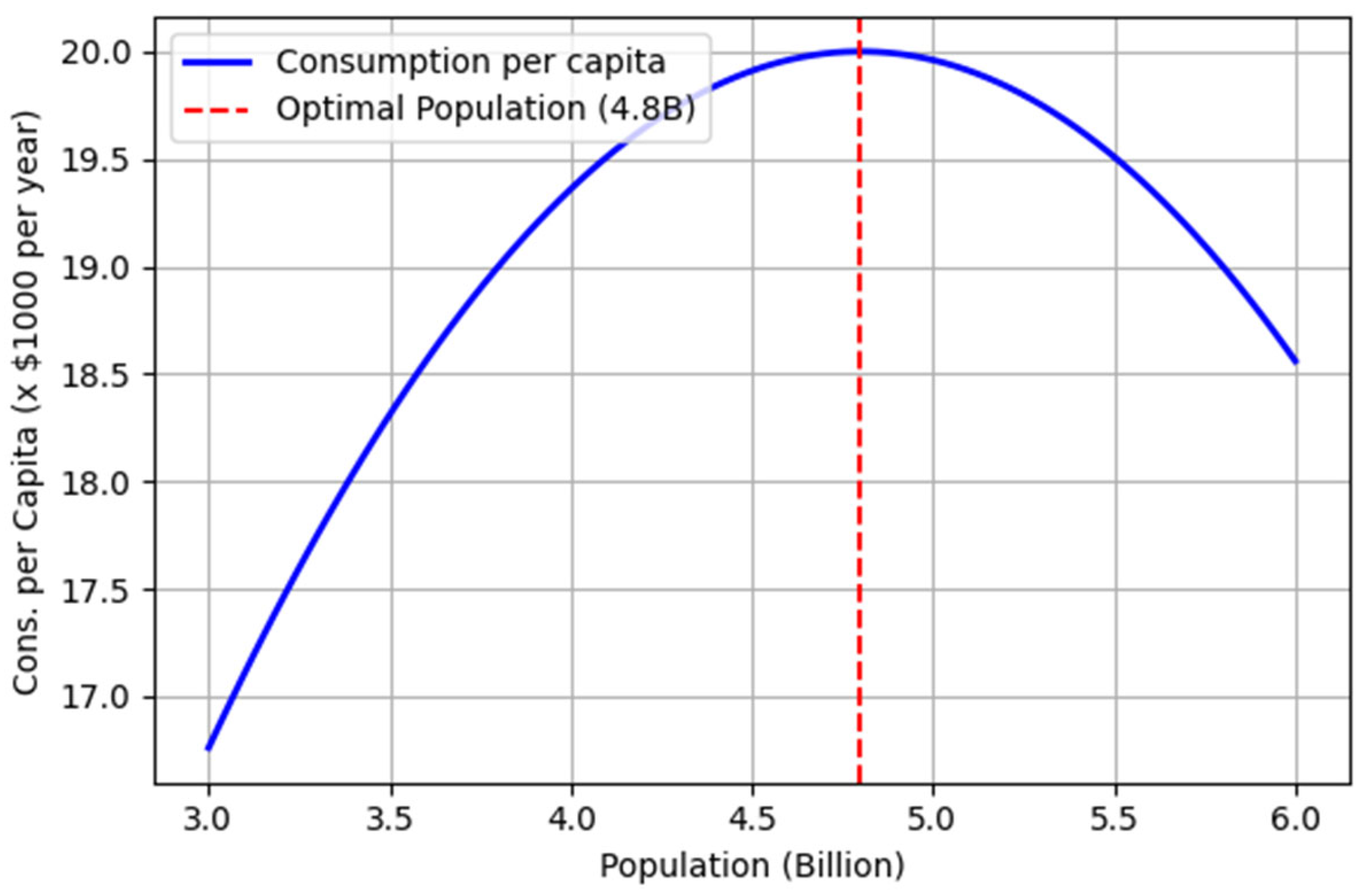
Figure 1. Optimal population versus per-capita consumption derived from model simulation.

Pollution Stock

AT the level of

P^{*} \approx 8.87 \times 10^{3}

(in index units), natural removal

ϕ P^{*}

exactly offsets the ongoing emissions, so the pollution stock is stable (neither growing nor shrinking). In this optimal scenario, anthropogenic emissions are dramatically reduced compared to a business-as-usual path, allowing the climate or environment to reach a new equilibrium. For context, external climate analyses often suggest that roughly an 80% cut in CO₂ emissions (relative to current levels) would be required to halt the increase in atmospheric CO₂ concentrations. Our model’s outcome of

τ^{*} \approx 0.33

corresponds to a one-third cut in gross emissions, which stabilizes pollution at a higher long-run concentration, relying on the fact that at the elevated

P^{*}

, natural sinks absorb the remaining two-thirds of emissions.

Figure @ref(fig:consPopGraph) illustrates how steady-state consumption per capita would vary with population in our model. In this simulation, consumption per person peaks at approximately 4.8 billion people, indicating the population size that yields the highest average living standard under the given technological and environmental parameters. Beyond this point, further increases in population lead to diminished per-capita resources and higher pollution burdens, causing average consumption to decline. This nonlinear relationship highlights the existence of an optimal population level (in terms of maximizing per-capita welfare) in a world with finite resources and pollution constraints.

Stability Analysis

Jacobian Matrix at the Steady State

To analyze local stability, we linearize the system around its dynamic equilibrium. Let

K^{*}, N^{*}, P^{*}

denote the steady-state values of capital, population, and pollution, and let

τ^{*}

and

c^{*}

be the steady-state abatement fraction and per-capita consumption. The Jacobian

J

is the

3 \times 3

(or

4 \times 4

including

c

) matrix of partial derivatives of the dynamic system with respect to the state variables. Including the consumption equation (via the Euler condition) for a full optimality analysis, our state vector is

(K, N, P, c)

.

The Jacobian matrix

J

around the steady state (with state order

(K, N, P, c)

) can be written symbolically as:

J =

Substituting the given parameter values and steady-state quantities into

J

yields a numerical Jacobian. The calibrated steady state is characterized by:

$α = 0.33$ , $δ = 0.05$ , $ρ = 0.02$ , $σ = 2.0$ .
$a = 0.20$ , $b = 1 \times 10^{- 5}$ , $ϕ = 0.01$ , $θ = 1.0$ .
$g_{0} = 0.015$ , and $P_{safe} \approx 8870$ (which gives $ψ = g_{0} / P^{*} \approx 1.69 \times 10^{- 6}$ ).
Steady-state technology $A^{*} = 5.36$ and population $N^{*} = 5.0 \times 10^{9}$ .

Plugging these values into the Jacobian, we obtain the following numerical matrix (elements in per-year units):

J \approx (\begin{matrix} 0.020 & - 2.08 & - 1.11 \times 10^{6} & - 5.00 \times 10^{9} \\ 0 & 0 & - 8.45 \times 10^{3} & 0 \\ 0 & 0 & - 0.010 & 0 \\ - 0.202 & 0 & - 1.45 \times 10^{- 5} & 0 \end{matrix}) .

Eigenvalues and Discussion

Finally, we compute the eigenvalues of the Jacobian matrix to assess the local stability of the equilibrium. The eigenvalues

λ_{i}

of

J

are approximately:

$λ_{1} \approx + 3.18 \times 10^{4},$
$λ_{2} \approx - 3.18 \times 10^{4},$
$λ_{3} \approx - 0.01,$
$λ_{4} \approx 0.00 .$

The dynamic equilibrium is saddle-path stable. The economy-environment system will converge to the steady state only if the controls

(c, τ)

are adjusted along the unique stable manifold. Two eigenvalues (including the crucial large one associated with consumption) are negative, ensuring convergence along those directions, while one positive eigenvalue indicates an unstable direction (requiring a jump in controls to avoid divergence).

The near-zero eigenvalue reflects the marginal stability of population at the environmental threshold. In practice, the planner’s optimal policy would manage this by adjusting

τ

to maintain the population close to

N^{*}

, ensuring that all relevant trajectories approach the steady state. The equilibrium can therefore be characterized as a saddle point with a one-dimensional unstable subspace (and a neutral/manifold direction due to population), which is typical for optimal growth models with a state constraint or threshold effect.

Conclusions

This paper develops a dynamic optimal growth model that explicitly integrates population dynamics, environmental constraints, and economic growth. The model identifies a critical pollution threshold, beyond which further environmental degradation halts population growth, potentially triggering societal collapse. At first glance, the finding that a smaller population supports higher per-capita welfare seems intuitive, given finite resources and environmental limits. However, upon deeper analysis, the model’s genuine contribution lies precisely in revealing and quantifying the complex trade-offs that shape the notion of an optimal rather than minimal population size.

Indeed, the intuitive notion that smaller populations yield higher individual consumption levels overlooks several counteracting forces that favor larger populations: economies of scale in production and infrastructure, deeper and more efficient markets, specialization advantages, and the enhanced generation of innovative ideas associated with greater human capital. Larger populations historically correlate with richer and more diverse economic networks, providing fertile ground for technological innovation, productivity gains, and improved overall economic performance.

Thus, the critical innovation of this study lies not in merely confirming the negative correlation between population size and per-capita resource availability, but rather in rigorously determining the precise balance point—the population level at which these competing forces are optimally reconciled. The result, identifying an optimal steady-state global population of approximately 3–5 billion individuals, represents neither a minimal nor maximal sustainable population, but an intermediate equilibrium where economies of scale, market depth, and innovation benefits are effectively balanced against environmental constraints and resource limitations.

Moreover, the paper contributes uniquely by explicitly modeling population as endogenously responsive to environmental conditions. By setting a rigorous environmental threshold and incorporating endogenous demographic dynamics, the analysis identifies an optimal policy strategy involving substantial but feasible pollution abatement efforts (around one-third of potential emissions). This optimal policy secures both environmental stability and sustained high per-capita welfare, thus clearly delineating a sustainable “green equilibrium.”

These results strongly challenge oversimplified policy narratives. Unrestricted demographic expansion or an exclusively technological optimism ignores crucial ecological limits, while simplistic advocacy for minimal populations underestimates the economic advantages derived from scale, specialization, and innovation. Instead, sustainable development policy should actively manage population dynamics and pollution levels, ensuring both ecological integrity and sufficient economic scale for robust markets and innovation-driven productivity growth.

In conclusion, the originality and significance of this research arise from its balancing of opposing forces: economies of scale and innovation benefits versus ecological and resource constraints, within a unified modeling framework. Future extensions could beneficially explore endogenous technological progress, innovation dynamics explicitly dependent on population size, and additional resource constraints, deepening our understanding of sustainable population levels and informing more nuanced and effective long-term economic and environmental policies.

Appendix 1. Model Derivations and Simulation

Model Framework

We consider a social planner model of the global economy with three key state variables: population

N (t)

, capital stock

K (t)

, and pollution stock

P (t)

. Time is continuous. The production function is Cobb–Douglas with labor (population) and capital as inputs. Pollution is a by-product of output but can be reduced by abatement efforts. The planner maximizes a discounted stream of utility, which depends on consumption per capita and possibly on environmental quality. The model’s structure is summarized by the following equations:

Production: $Y (t) = A, K {(t)}^{α}, N {(t)}^{, 1 - α}$ , where $0 < α < 1$ is the capital share and $A$ is total factor productivity (assumed constant).
Capital accumulation: $\dot{K} (t) = Y (t) - C (t) - Π (t) - δ K (t)$ . Here $C (t)$ is total consumption, $Π (t)$ is total resources devoted to pollution abatement, and $δ$ is the capital depreciation rate. In other words, output is allocated to consumption, abatement, and maintaining capital.
Abatement and pollution: Let $μ (t)$ be the abatement effort, defined as the fraction of output devoted to abatement ( $Π = μ Y$ ). The remaining fraction $(1 - μ)$ of output is the effective output for consumption and investment. Pollution accumulates according to $\dot{P} (t) = Φ, Y (t), (1 - μ (t)) - s, P (t)$ , where $Φ$ is an emission factor (pollution produced per unit of output) and $s$ is the natural pollution absorption rate. In steady state, emissions $Φ (1 - μ) Y$ equal natural absorption $s P$ .
Population dynamics: Population grows according to $\dot{N} (t) = N (t), [b - d (P (t))]$ . Here $b$ is an exogenous birth rate and $d (P)$ is the death (mortality) rate, assumed to increase with pollution (environmental damage raises mortality). This captures a “positive check” where pollution reduces population by increasing mortality. In steady state, $\dot{N} = 0$ requires $b = d (P^{*})$ , so the steady-state pollution $P^{*}$ is that which raises the death rate enough to offset births, yielding a stable population $N^{*}$ .
Utility: The planner’s objective at time $0$ is ${m a x}_{C (t), μ (t), b (t)} \int_{0}^{\infty} e^{- ρ t} U (C (t), N (t), P (t)) d t,$ where $ρ \geq 0$ is the pure rate of time preference. We assume utility per capita takes a form $u (c) - D (P)$ , increasing in consumption per person $c = C / N$ and decreasing in pollution. A convenient specification (used for numerical examples) is logarithmic utility and linear disutility of pollution: $U (C, N, P) = N [l n (c) - γ P] = N l n (c) - γ N P,$ where $γ > 0$ is the weight of pollution disutility. This implies diminishing marginal utility of consumption and a linear “damage” from pollution. (In words, each person suffers disutility $γ P$ from the pollution stock.) The term $N l n (c)$ corresponds to a total utilitarian welfare criterion, where having more people can increase total utility, subject to the environmental and capital constraints. The model thus captures the fundamental trade-off: adding an extra person provides utility benefits but also imposes costs by diluting capital and increasing pollution.

Sustainability: A path is sustainable if consumption never decreases and population does not decline over time. We focus on a steady state that satisfies this sustainability criterion (non-declining

C

and

N

). In steady state,

\dot{K} = \dot{N} = \dot{P} = 0

, and all variables remain constant. Below, we derive the conditions characterizing the optimal steady state

(N^{*}, K^{*}, P^{*}, C^{*}, μ^{*})

that maximizes welfare subject to the model constraints.

Steady-State Conditions and Derivations

In a steady state, population, capital, and pollution are constant. We denote steady-state values with asterisks. The steady-state conditions are:

Population: $\dot{N} = 0$ implies $b = d (P^{*})$ . Thus the steady-state pollution stock $P^{*}$ is implicitly determined by $d (P^{*}) = b$ . (If $d (P)$ is increasing, this pins down a unique $P^{*}$ .) The corresponding population $N^{*}$ is whatever level is consistent with that pollution stock given economic decisions. In other words, $N^{*}$ will adjust until the pollution-induced mortality equals the birth rate in steady state.
Pollution: $\dot{P} = 0$ implies $Φ, (1 - μ^{*}) Y^{*} = s, P^{*}$ . This means the steady stock $P^{*}$ is $P^{*} = \frac{Φ (1 - μ^{*}) Y^{*}}{s},$ i.e. the ratio of sustained emissions to the natural absorption rate. Intuitively, higher abatement $μ^{*}$ or lower output $Y^{*}$ reduces the pollution stock needed to balance outflows.
Capital: $\dot{K} = 0$ implies $(1 - μ^{*}) Y^{*} - C^{*} = δ K^{*}$ . The term $(1 - μ^{*}) Y^{*}$ is output net of abatement costs, which is used for either consumption or investment. In steady state, net investment must equal depreciation $δ K^{*}$ just to maintain the capital stock. Equivalently, $C^{*} = (1 - μ^{*}) Y^{*} - δ K^{*} .$ This equation will be used along with the optimality conditions to solve for $C^{*}$ and $K^{*}$ .

Next, we use the optimality (first-order) conditions for the planner’s control variables

(C, μ, b)

in steady state. We set up the current-value Hamiltonian for the planner’s problem:

H = N [l n (c) - γ P] + λ ((1 - μ) Y - C - δ K) + η (Φ (1 - μ) Y - s P) + ξ N (b - d (P)),

with co-state (shadow price)

λ (t)

for capital,

η (t)

for pollution, and

ξ (t)

for population. In steady state, the FOCs and co-state equations yield the conditions below. (For brevity, we focus on interior solutions where

C, μ, N

are positive and finite.)

Consumption Euler equation: $\partial H / \partial C = 0$ gives $\frac{\partial}{\partial C} [N l n (c)] - λ = 0$ . Since $c = C / N$ , $\partial (N l n c) / \partial C = \frac{N}{C} = \frac{1}{c}$ . Thus $λ = \frac{1}{c^{*}} .$ The shadow price of capital $λ$ equals the marginal utility of consumption. In steady state, the co-state dynamics $\dot{λ} = ρ λ - \partial H / \partial K$ must also hold. At steady state $\dot{λ} = 0$ , so $ρ λ = λ [δ + O_{K}] - λ \partial (N l n c) / \partial K$ (where $O_{K}$ is output’s derivative w.rt $K$ ). Solving this yields the modified golden-rule condition: $f_{K} (K^{*}, N^{*}) = ρ + δ .$ Here $f_{K} = \partial Y / \partial K = α A {(K / N)}^{α - 1}$ is the marginal product of capital. If $ρ = 0$ (zero pure time preference, a case often examined for sustainability), this simplifies to $f_{K} (K^{*}, N^{*}) = δ .$ This is the classic golden rule condition: at optimum, capital per worker is such that the marginal product of capital equals the depreciation rate. Intuitively, this maximizes consumption per capita in steady state. We assume $ρ$ is small; hence we will use $f_{K} \approx δ$ in numerical simulations (the difference between $ρ = 0$ and a small $ρ$ would be minor for our purposes).
Abatement condition: $\partial H / \partial μ = 0$ gives $- λ Y^{*} + η Φ Y^{*} = 0 ⟹ η = \frac{λ}{Φ} .$ This equates the marginal utility cost of abating (lost output $\Rightarrow$ lost utility $λ Y$ ) to the marginal utility benefit (reduced pollution $\Rightarrow$ utility gain $η, Φ Y$ ). Substituting $λ = 1 / c^{*}$ , we get $η = \frac{1}{Φ c^{*}} .$ The co-state $η$ can be interpreted as the shadow cost of pollution in utility terms. Meanwhile, the co-state equation for $η$ at steady state yields $ρ η = γ N^{*} - η s$ , i.e. $η (s + ρ) = γ N^{*}$ . For small $ρ$ , approximately $η s = γ N^{*}$ in steady state – the shadow cost of pollution $η$ adjusts until the marginal disutility $γ N^{*}$ from an extra unit of $P$ (felt by $N^{*}$ people) is balanced by the discounted future dilution of that pollution via natural decay $s$ . Combining this with $η = 1 / (Φ c^{*})$ , we obtain an implicit formula for optimal abatement effort $μ^{*}$ : $\frac{1}{Φ c^{*}} \approx \frac{γ N^{*}}{s} \Rightarrow Φ c^{*} \approx \frac{s}{γ N^{*}} .$ Rearranging, and noting $c^{*} = (1 - μ^{*}) Y^{*} / N^{*}$ , this condition can be expressed as a ratio of abatement cost to output:

$\frac{μ^{*}}{1 - μ^{*}} = \frac{γ Φ Y^{*} N^{*} / s}{N^{*} / c^{*}} = \frac{γ Φ Y^{*}}{s / c^{*}} \approx \frac{γ N^{*}}{(1 - μ^{*})},$

after simplifying $c^{*}$ and canceling $N^{*}$ . (In simpler terms, the planner equalizes the percentage of output spent on abatement to a function of population and pollution parameters. A higher population or higher pollution damage $γ$ calls for greater abatement effort $μ^{*}$ , ceteris paribus.)

Interpretation: The optimal abatement

μ^{*}

satisfies

Marginal Benefit of Abatement = Marginal Cos t of Abatement

. Marginal cost is the output loss $1 yields

λ = 1 / c

utils; marginal benefit is the reduction of pollution by

Φ

units, which yields

η, Φ = λ

utils (from

η = λ / Φ

). Thus at optimum, spending another dollar on abatement would yield the same utility as spending it on consumption – this pins down

μ^{*}

.

Population (fertility) condition: $\partial H / \partial b = 0$ yields $ξ = 0$ (since $b$ only appears in $ξ N b$ term). The co-state $ξ$ for population evolves as $\dot{ξ} = ρ ξ - \partial H / \partial N$ . Setting $\dot{ξ} = 0$ and using $ξ = 0$ , we get $\partial H / \partial N = 0$ in steady state. This is the optimal population condition: $\frac{\partial}{\partial N} [N (l n c - γ P)]_{N = N^{*}} = 0 .$ Expanding the derivative gives $l n c^{*} - γ P^{*} + N^{*} (\frac{\partial l n c}{\partial N} - γ \frac{\partial P}{\partial N}) = 0 .$ In steady state $c = C / N$ and $C = (1 - μ) Y - δ K$ , so an extra person affects $c$ by diluting resources (capital) slightly; however, if the production function has constant returns, $c$ is roughly independent of $N$ when $K$ adjusts proportionally. We assume the dominant effect is through pollution: more people raise pollution (since $P^{*} \propto N^{*}$ in steady state for given $μ$ and $Y / N$ ). Thus, approximately, $\partial l n c / \partial N \approx 0$ (constant returns) while $\partial P / \partial N = \frac{Φ (1 - μ^{*}) Y^{*}}{s} \frac{1}{N^{*}} = \frac{P^{*}}{N^{*}}$ . Using these simplifications, the optimal population condition reduces to $l n c^{*} = γ \frac{\partial}{\partial N} [N P^{*}] \approx γ (P^{*} + N^{*} \frac{P^{*}}{N^{*}}) = 2 γ P^{*} .$ Thus, the planner adds people until the utility gain of an extra person ( $l n c$ ) equals the disutility they impose via pollution ( $2 γ P$ ). The factor 2 arises because an extra person not only experiences pollution (cost $γ P$ to themselves) but also contributes to total pollution harming everyone (an additional $γ N \frac{\partial P}{\partial N} \approx γ P$ to all others). Setting these equal yields the condition $l n (c^{*}) = 2 γ P^{*}$ . This implicit equation determines $N^{*}$ in relation to $P^{*}$ and $c^{*}$ . Substituting $P^{*} = Φ (1 - μ^{*}) Y^{*} / s$ and $c^{*} = C^{*} / N^{*}$ gives an explicit solvable form for $N^{*}$ (see below).

Putting the above conditions together, we have a system of equations for

(K^{*}, N^{*}, P^{*}, μ^{*}, C^{*})

. It is convenient to express these in terms of intensive (per capita) variables using

k = K / N

and

y = Y / N

:

Optimal capital per person: $f_{K} = α A k^{α - 1} = ρ + δ$ . For $ρ \approx 0$ , this gives $α A k^{α - 1} = δ ⟹ k^{*} = (\frac{α A}{δ})^{\frac{1}{1 - α}} .$ This is the golden-rule $k^{*}$ that maximizes output per person net of depreciation. (Note that $k^{*}$ is independent of $N$ under constant returns and $ρ = 0$ .) The corresponding output per person is $y^{*} = A {(k^{*})}^{α}$ .
Consumption and output: In steady state, $C = (1 - μ) Y - δ K$ . Dividing by $N$ gives $c = (1 - μ) y - δ k$ . Using $f_{K} = δ$ , one can show $δ k = α (1 - μ) y$ , so that $c^{*} = (1 - μ^{*}) (1 - α) y^{*} .$ Thus consumption per capita is a fraction $(1 - α)$ of net output per capita $(1 - μ) y^{*}$ – intuitively, $(1 - α)$ is labor’s share of net output, which is available for consumption after replacing depreciated capital (which costs fraction $α$ of net output).
Pollution stock: $P^{*} = \frac{Φ (1 - μ^{*}) Y^{*}}{s} = \frac{Φ (1 - μ^{*}) y^{*} N^{*}}{s}$ .
Optimal abatement: The planner’s first-order condition can be rearranged (as discussed above) into an implicit formula for $μ^{*}$ . Using $1 / c^{*} = η Φ$ and $η s = γ N^{*}$ , we eliminate $η$ to get $\frac{1}{c^{*}} \frac{s}{Φ} = γ N^{*} .$ Substituting $c^{*} = (1 - μ^{*}) (1 - α) y^{*}$ and $y^{*} = A {(k^{*})}^{α}$ , this condition becomes: $\frac{s}{Φ (1 - μ^{*}) (1 - α) y^{*}} = γ N^{*} .$ This implicitly defines $μ^{*}$ as a function of $N^{*}$ (and other parameters). In general, one must solve this equation along with the population optimum condition for $μ^{*}$ and $N^{*}$ .
Optimal population: Using $l n c^{*} = 2 γ P^{*}$ (derived above), and substituting $c^{*}$ and $P^{*}$ from (2) and (3), we obtain: $l n ((1 - μ^{*}) (1 - α) y^{*}) = 2 γ \frac{Φ (1 - μ^{*}) y^{*} N^{*}}{s} .$ This equation can be solved for $N^{*}$ given $y^{*}$ and $μ^{*}$ . Cancelling the common factor $(1 - μ^{*}) y^{*}$ (which is positive in a non-trivial steady state), we can rewrite it as: $l n ((1 - α) y^{*}) + l n (1 - μ^{*}) = \frac{2 γ Φ y^{*}}{s} N^{*} .$ Notice that $(1 - α) y^{*}$ is essentially the output per person available for consumption if $μ = 0$ (no abatement). This equation shows that the optimal population is smaller when pollution damage $γ$ is larger or natural absorption $s$ is lower, and it is larger when productivity $y^{*}$ is higher. In words: more productive economies can sustain a larger population, but higher environmental sensitivity or lower planetary resilience push the optimal population down.

Solving equations (4) and (5) simultaneously determines

N^{*}

and

μ^{*}

(the other variables

k^{*}, y^{*}, c^{*}, P^{*}

then follow directly). Analytical solutions are complicated, so we turn to numerical simulation to find these optimal values.

Simulation

Here is a step-by-step reconstruction of the numbers in lines 399–426.

Parameters Used

Output at steady state: $Y^{*} = 132$ trillion USD (we measure $Y$ in “trillions of USD” when used in the pollution equation to keep units consistent)
Population: $N^{*} = 5.0 \times 10^{9}$ people
Depreciation: $δ = 0.05$
Investment share: $s = 0.24$
Abatement cost coefficient: $a = 0.20$ in $a τ^{2} Y$
Optimal abatement: $τ^{*} = 0.33$
Natural removal rate of pollution: $ϕ = 0.01$
Emission intensity (unit choice): $θ = 1.0$
Steady-state pollution stock: $P^{*} \approx 8.87 \times 10^{3}$ (index units)
Damage coefficient (chosen so damage is a fraction of output): $b = 10^{- 5}$ so that $b P^{*} \approx 0.0887$ i.e., 8.87% of output
Baseline net population growth: $g_{0} = 0.015$

Capital Stock $K^{*}$

Steady-state capital balance:

\dot{K} = 0 \Rightarrow s Y^{*} = δ K^{*} \Rightarrow K^{*} = \frac{s}{δ} Y^{*} .

K^{*} = \frac{0.24}{0.05} \times 132 = 4.8 \times 132 = 633.6 trillion USD \approx 636 t r i l l i o n .

Pollution Balance and $τ^{*}$

Steady-state pollution:

\dot{P} = 0 \Rightarrow θ (1 - τ^{*}) Y^{*} = ϕ P^{*} .

Using

θ = 1

,

τ^{*} = 0.33

,

Y^{*} = 132

(trillions),

ϕ = 0.01

,

P^{*} = 8870

:

(1 - 0.33) \times 132) \approx 0.01 \times 8870 .

LHS and RHS match within rounding. This shows the chosen

τ^{*}

,

Y^{*}

, and

P^{*}

are mutually consistent in steady state given our unit choice (measuring

Y

in “trillions”).

Total Consumption $C^{}$ and Per-Capita $c^{}$

The paper’s accounting for consumption (money units) is

C = [1 - s - a τ^{2}] Y - damage .

With damage modeled as a fraction of output, the fraction is

b P

. Thus,

C^{*} = (1 - s - a {τ^{*}}^{2} - b P^{*}) Y^{*} .

Compute each term:

Abatement fraction: $a {τ^{*}}^{2} = 0.20 \times {0.33}^{2} = 0.20 \times 0.1089 = 0.02178$ (≈ 2.178% of $Y$ )
Damage fraction: $b P^{*} = 10^{- 5} \times 8870 = 0.0887$ (≈ 8.87% of $Y$ )
Consumption share of output:

$1 - s - a {τ^{*}}^{2} - b P^{*} = 1 - 0.24 - 0.02178 - 0.0887 = 0.64952 (\approx 64.95 %) .$

Therefore,

$C^{*} = 0.64952 \times 132 = 85.735 trillion USD .$

Per-capita consumption:

$c^{*} = \frac{C^{*}}{N^{*}} = \frac{85.735 \times 10^{12}}{5.0 \times 10^{9}} = 17,147 USD / person / year \approx 17,200 .$

Population Condition and $ψ$

The demographic equation is

\dot{N} = N (g_{0} - ψ P) .

At steady state,

\dot{N} = 0 \Rightarrow P^{*} = g_{0} / ψ

, so

ψ = \frac{g_{0}}{P^{*}} = \frac{0.015}{8870} \approx 1.69 \times 10^{- 6} per pollution unit .

This is the sensitivity that makes the long-run population growth rate zero at

P^{*}

. The choice of

N^{*} \approx 5

billion comes from your optimality analysis and numerical search: per-capita consumption peaks around that population given the sustainability constraint and abatement policy, so the paper reports that value as the welfare-maximizing sustainable population.

References

Arrow, K. J., Dasgupta, P., Goulder, L. H., Daily, G. C., Ehrlich, P. R., Heal, G. M., Levin, S. A., Mäler, K.-G., Schneider, S. H., Starrett, D. A., & Walker, B. (2004). Are we consuming too much? Journal of Economic Perspectives, 18(3), 147–172. [CrossRef]
Brander, J. A., & Taylor, M. S. (1998). The simple economics of Easter Island: A Ricardo-Malthus model of renewable resource use. American Economic Review, 88(1), 119–138.
Ehrlich, P. R., & Holdren, J. P. (1971). Impact of population growth. Science, 171(3977), 1212–1217. [CrossRef]
Global Footprint Network. (2022). National footprint accounts 2022 edition. Retrieved from https://data.footprintnetwork.org.
Hartwick, J. M. (1977). Intergenerational equity and the investing of rents from exhaustible resources. American Economic Review, 67(5), 972–974.
Kremer, M. (1993). Population growth and technological change: One million B.C. to 1990. Quarterly Journal of Economics, 108(3), 681–716. [CrossRef]
Lehmijoki, U., & Rovenskaya, E. (2007). Optimal pollution and optimal population (IIASA Interim Report IR-07-023). Laxenburg, Austria: International Institute for Applied Systems Analysis. Retrieved from http://pure.iiasa.ac.at/8434.
Lianos, Theodore P. 2022. “Population and Steady-State Economy in Plato and Aristotle.” Journal of Population and Sustainability 7 (1). [CrossRef]
Malthus, T. R. (1798). An essay on the principle of population, as it affects the future improvement of society. London: J. Johnson.
Meadows, D. H., Meadows, D. L., Randers, J., & Behrens, W. W. III. (1972). The limits to growth: A report for the Club of Rome’s project on the predicament of mankind. New York: Universe Books.
Nordhaus, W. D. (1994). Managing the global commons: The economics of climate change. Cambridge, MA: MIT Press.
Simon, J. L. (1980). Resources, population, environment: An oversupply of false bad news. Science, 208(4451), 1431–1437. [CrossRef]
Solow, R. M. (1974). Intergenerational equity and exhaustible resources. Review of Economic Studies, 41, 29–45. [CrossRef]
Stiglitz, J. E. (1974). Growth with exhaustible natural resources: Efficient and optimal growth paths. Review of Economic Studies, 41, 123–137. [CrossRef]
United Nations. (2022). The Sustainable Development Goals Report 2022. New York: United Nations.
United Nations Department of Economic and Social Affairs, Population Division. (2022). World population prospects 2022: Summary of results. New York: United Nations.
United Nations Environment Programme. (2024). Emissions Gap Report 2024: No more hot air … please! Nairobi: UNEP.
World Economic Forum. (2024). The global risks report 2024 (19th ed.). Geneva: World Economic Forum.

Table 1. Model Variables and Parameters.

Symbol	Description	Units or Notes
$K (t)$	Physical capital stock	Monetary units
$N (t)$	Population (number of people)	Individuals
$P (t)$	Pollution stock	Pollution units
$A (t)$	Technology level	Productivity index
$Y (t)$	Economic output (GDP)	Monetary units per year
$C (t)$	Consumption	Monetary units per year
$τ (t)$	Abatement effort (fraction of output)	Fraction
$α$	Output elasticity of capital	Dimensionless
$θ$	Pollution emitted per unit output	Pollution units per output
$ϕ$	Pollution natural decay rate	Per year
$P_{safe}$	Safe pollution threshold (collapse level)	Pollution units (e.g., ppm CO₂)
$g_{0}$	Baseline population growth rate	Per year
$ψ$	Population sensitivity to pollution	Per pollution unit per year
$δ$	Depreciation rate of capital	Per year
$s$	Investment (saving) rate	Fraction of output
$ρ$	Social discount rate	Per year
$σ$	Elasticity of marginal utility (CRRA)	Dimensionless

Disclaimer/Publisher’s Note: The statements, opinions and data contained in all publications are solely those of the individual author(s) and contributor(s) and not of MDPI and/or the editor(s). MDPI and/or the editor(s) disclaim responsibility for any injury to people or property resulting from any ideas, methods, instructions or products referred to in the content.

© 2025 by the authors. Licensee MDPI, Basel, Switzerland. This article is an open access article distributed under the terms and conditions of the Creative Commons Attribution (CC BY) license (http://creativecommons.org/licenses/by/4.0/).

Copyright: This open access article is published under a Creative Commons CC BY 4.0 license, which permit the free download, distribution, and reuse, provided that the author and preprint are cited in any reuse.

Optimal Population and Sustainable Growth Under Environmental Constraints

Abstract

Keywords:

Subject:

Introduction

Literature Review

The Model

Production

Pollution and Environmental Constraint

Capital Accumulation and Consumption

Population Dynamics

Utility and Welfare Objective

Model Calibration and Sustainable Population Estimate

Population Growth Parameters

Production and Technology Parameters

Pollution and Abatement Parameters

Optimal Population: An Empirical View

Optimal Control Solution

First-Order Conditions (FOCs)

Consumption vs Investment

Pollution Abatement ( τ )

Population

Steady State

Population

Output (GDP)

Capital Stock

Consumption per Capita

Abatement Effort

Pollution Stock

Stability Analysis

Jacobian Matrix at the Steady State

Eigenvalues and Discussion

Conclusions

Model Framework

Steady-State Conditions and Derivations

Simulation

Parameters Used

Capital Stock K *

Pollution Balance and τ *

Total Consumption C * and Per-Capita c *

Population Condition and ψ

References

MDPI Initiatives

Important Links

Subscribe

Pollution Abatement ( $τ$ )

Capital Stock $K^{*}$

Pollution Balance and $τ^{*}$

Total Consumption $C^{}$ and Per-Capita $c^{}$

Population Condition and $ψ$