Submitted:
29 August 2025
Posted:
01 September 2025
You are already at the latest version
Abstract
Background/Objectives Breast cancer (BC) remains the most prevalent cancer among women, and its effective treatment relies heavily on early detection. To our knowledge, this is the first study to integrate serum tryptophan fluorescence data with Gaussian Process Regression (GPR) and validate findings through confocal and histopathological imaging. Optical techniques are employed to assess fluorescence variations of key endogenous biomolecules, including tryptophan, Reduced Nicotinamide Adenine Dinucleotide (NADH), and Flavin Adenine Dinucleotide (FAD), which play vital roles in cellular metabolism. Changes in their concentrations are associated with malignancy. The objective is to distinguish between normal and cancerous breast tissues based on tryptophan fluorescence spectra. Methods Intrinsic fluorescence spectra of tryptophan, NADH, and FAD were acquired and compared to assess their potential for distinguishing between normal and cancerous conditions. Among them, tryptophan fluorescence intensity in serum emerged as the most effective marker for differentiation. GPR and other potential models were applied to predict cancer status based on serum fluorescence data, with model performance evaluated using standard error metrics such as root mean squared error (RMSE). Additionally, confocal autofluorescence imaging of breast tissue samples was performed and compared with Hematoxylin and Eosin (H&E)-stained Differential Interference Contrast (DIC) images to validate morphological differences and support the method’s effectiveness. Results The findings reveal a clear distinction between normal and cancerous breast tissues based on serum tryptophan fluorescence intensity. Spectral analysis confirmed that tryptophan, along with NADH and FAD, effectively reflects malignancy-associated metabolic alterations. Among the models tested, GPR outperformed with the highest predictive accuracy, with RMSEs of 1847.5 (range: 2 × 10⁶) for normal and 3621.6 (range: 6 × 10⁶) for cancerous samples, both constituting less than 0.1% of their respective fluorescence intensity ranges. Conclusions Serum tryptophan fluorescence intensity has been identified as a robust biomarker for distinguishing between normal and cancerous breast tissues. The integration of optical spectral data with the GPR model yielded high predictive accuracy, demonstrating the method’s effectiveness in identifying malignancy. The results were supported by stained and confocal imaging. These findings support the development of a non-invasive, real-time screening method that could reduce reliance on traditional histopathological diagnostics and serve as a rapid, cost-effective adjunct to biopsy and mammography in early BC detection.
Keywords:
fluorescence spectroscopy
; tryptophan
; breast cancer
; confocal microscopy
; integrating sphere
; machine learning
1. Introduction
Breast cancer (BC) is the most commonly occurring cancer among women, with nearly 2.3 million women worldwide [1,2]. Its early diagnosis improves the patient's chances of survival [3]. Mammography, ultrasound imaging, magnetic resonance imaging (MRI), and breast biopsy are traditional methods of BC diagnosis [4,5,6]. These traditional methods carry false-positive/false-negative errors [7]. Mammography uses X-ray radiation, which is harmful to human health [8,9,10]. Ultrasound relies on specialist knowledge and has less sensitivity [11]. MRI is expensive, has low resolution, and does not identify the type of cancer [12]. Biopsy is the gold standard method. However, surgical procedures require biopsies and take months, including multiple biopsies [13]. Raman spectroscopy can make real-time detection, but due to the nonlinearity of detectors, device development is complicated [14].
The above-mentioned traditional diagnosis methods are cumbersome, uneconomical, physician experience-dependent, and invasive. An efficient, economical, and real-time method for the early diagnosis of BC is the need of the present medicine market. Modern science is constantly looking for more accurate, non-invasive, economical, and real diagnostic techniques. Optical methods have made an excellent step for early BC diagnosis and are non-invasive, reliable, and highly sensitive [15,16]. Optical methods include diffuse scattering, absorption, Muller matrix polarimetry, fluorescence spectroscopy, and microscopy. Among optical methods, fluorescence spectroscopy and microscopy have a significant role based on volume investigation and application of results [17].
Intrinsic fluorophores in tissues include amino acids, structural proteins, enzymes and coenzymes, vitamins, lipids, and porphyrins. Every fluorophore has its unique excitation and emission spectra across the whole spectral region.
Fluorescence spectroscopy based on tryptophan biomarkers provides a real-time and rapid solution for early diagnosis of BC. A specific wavelength of light λ is used to illuminate intrinsic fluorophores, such as tryptophan. It absorbs light and emits light longer λ having a stock shift of Δλ = 20 nm.
A combination of experimental methods and machine learning (ML) models is the need of the present to make a diagnosis device for BC diagnosis and has been used for mitosis detection [18]. ML-based regression analysis has remained a reliable tool for quite some time in numerous fields of science. It has been used for mitosis counting using deep learning (DL) strategies [19]. The framework’s main features are the down-sampling and upsampling paths, making end-to-end training feasible. DL requires enormous amounts of data compared to ML techniques. Various regression modules along with ML have been used for BC diagnosis, including decision trees, multi-layer perceptron, random forest, and k-nearest neighbors' regressor. Wisconsin BC dataset based on 569 digital images of fine needle aspirate of breast and extracted ten real-valued features [20]. Using clinical data, ML models have been employed to predict BC survival time [21]. The datasets used in their study were integrated with no data loss. Accurate results were claimed using lasso regression, kernel ridge regression, k-neighborhood regression, and decision tree regression. Features like size and stage of tumor with age at the time of diagnosis were used.
In our study, appropriate excitation wavelengths for the targeted endogenous fluorophore, namely tryptophan, Reduced Nicotinamide Adenine Dinucleotide (NADH), and Flavin Adenine Dinucleotide (FAD) were used, and their fluorescence emission spectra were measured through conventional methods. Confocal autofluorescence imaging was performed on normal and cancerous breast tissues and Hematoxylin and Eosin (H&E) stained differential interference contrast (DIC) images were validated. Experimental fluorescence data plots of tryptophan, NADH, and FAD have been acquired from normal and BC patients and ML techniques have been employed for regression analysis of biomarkers. Regression-based validation and prediction analysis for tryptophan, NADH, and FAD (normal/ cancerous cases) has included using Gaussian process regression (GPR), wide neural networks (WNN), support vector regression (SVR), fine decision tree (FDT), and boosted tree (BT) models. The bi-feature approach was used to assign predictor and response variables for the regression analysis. This is a sufficiently informative process to provide tissue differentiation for rapid optical BC screening.
The rest of this paper is structured as follows: the Materials and Methods section describes the sample preparation process, spectral measurements, regression models utilized in this study, and the performance metrics applied for regression evaluation. The Results and Discussion section details the predictive capabilities of the models and examines how different configurations affect performance. The Conclusion section highlights the key findings and proposes potential directions for future investigation.
2. Materials and Methods
This study involved the collection of 300 BC specimens from women who underwent modified radical mastectomies at PIMS and PAEC hospitals between May 2020 and October 2023. The tissue samples, along with serum from patients under the age of 50, were processed and analyzed for histopathological classification, including invasive ductal carcinoma, invasive lobular carcinoma, and other tumor variants. After histopathological grading, fluorescence spectra measurements were performed on cancerous and normal tissues using a Fluorescence Spectro FluoroMax 4.0, capturing excitation-emission matrix (EEM) data. Regression models such as GPR, were then employed to analyze the spectra data. These models aimed to predict cancerous tissue characteristics based on the fluorescence data. Performance measures, namely, root mean squared error (RMSE), mean squared error (MSE), R-squared (R²), and mean absolute error (MAE), were utilized to evaluate the accuracy and fit of the regression models. These comprehensive analyses help to deepen the understanding of BC pathology by linking spectral data with tumor classifications, offering valuable insights for more accurate and intelligent cancer diagnostics.
2.1. Sample Preparation and Histopathological Review
We collected 300 BC specimens from women undergoing modified radical mastectomy for operable primary BC between May 2020 and October 2023. All BC tissues were collected from surgeries performed at the Pakistan Institute of Medical Sciences (PIMS), Islamabad, and the Pakistan Atomic Energy Commission (PAEC) General Hospital, Ni-lore, Islamabad.
Histopathology was based on hematoxylin and eosin (H&E) stained slides. The pathology specimens were reviewed independently by histopathologists to grade and sub-classify the tumors based on established criteria without knowledge of immunohistochemical results. Discrepancies in diagnoses were resolved by consensus with simultaneous viewing. All invasive carcinomas were graded using the Nottingham grading system of Elston and Ellis. After a final histopathologic review, 300 BC cases were further studied, including 200 cases of invasive ductal carcinoma (IDC) and ductal special types (tubular, mucinous); 50 cases of ILC and variants; 10 cases of tubulolobular carcinoma (TLC); and 40 cases of invasive carcinoma (IC), with uncertain classification between lobular and ductal type. Data on patient demographics, tumor size, and axillary lymph node status, stage of disease, ER and PgR status, and HER’s-2/neu overexpression were abstracted from the histopathology reports.
The serum samples and tissue slides of confirmed BC patients used in this study were collected from the Pakistan Institute of Medical Sciences (PIMS), Islamabad, and the Pakistan Atomic Energy Commission (PAEC) General Hospital, Nilore, Islamabad, along with normal patients for samples as control during October 2023 after ethical and legal permission. The study was approved by the Ethical Research Review Committee under document number F5-2 /2023/ERRC/PIMS dated 02/10/2023. Three hundred confirmed BC female patients under the age of 20-50 years were selected, and their blood sera and selected tissue slide data were collected and analyzed. Malignant and normal tissues were collected soon after the patients' surgical resection, and their fluorescence measurements were performed. Samples dimensions vary from 0.2×0.5×0.5 cm3 to 0.3×1.0×1.5 cm3 in the case of tissue slides, and in the case of sera, a 10 mm path length UV cuvette was used. Furthermore, H&E stained slides, as well as fresh slides, were prepared for confocal imaging of normal and BC patients. All the experiments were performed on sera and slide tissues at a controlled room temperature, which is 37 degrees Celsius.
2.2. Spectra Measurement
Fluorescence spectra were measured at room temperature using a Fluorescence Spectro Fluoro max 4.0. The spectra were collected in two phases: a) excitation range from 250 nm to 400 nm and emission range from 300 nm to 450 nm to obtain excitation emission matrix (EEM) as illustrated in Figure 1(a). The peak auto-fluorescence intensity of 0.5 M tryptophan solution measured using Horiba FluoroMax 4 Spectrofluorometer showed a peak at 380 nm when excited at 280 nm has been illustrated in Figure 1(b). Data recorded at a 150 nm/min scan rate. Xenon discharge lamp is used for illumination, and a gated red-sensitive R928 photomultiplier operating up to 900 volts is used for signal detection. The pattern of spectral curves' intensities is analyzed numerically, and the data is used in statistical regression analysis. Statistical analysis was performed using open-source Python libraries on GPU-based systems. Once the EEM excitation emission spectra optimal values are obtained, in the second phase, these optimum values are used to excite tryptophan, NADH, and FAD present in all the samples.
2.3. Regression Models
Following a spot check of several ML-based regression models, a concise summary of the regression models used for the analysis is presented.
2.3.1. GPR-Model 1
GPR is a Bayesian, non-parametric approach used for numeric fitting in ML [22]. It is particularly useful for regression tasks involving datasets with limited instances. Unlike traditional parametric models, GPR does not assume a fixed form for the underlying function. Instead, it infers the function’s form from the data, making it highly adaptable to complex, non-linear relationships. By defining a prior over possible functions and updating this with observed data using Bayes' Theorem, GPR provides a probabilistic framework that naturally incorporates uncertainty into predictions. The core of GPR lies in the choice of covariance function (kernel), which encodes assumptions about the smoothness and structure of the function. This allows the model to capture different types of relationships within the data. GPR is especially valuable in cases where data is sparse, as it exploits the data’s inherent structure through the kernel, making it effective even with fewer samples.
Unlike many popular supervised ML algorithms that learn exact values for every parameter in a function, the Bayesian approach infers a probability distribution over all possible values. Let's assume a linear function. How the Bayesian approach works by specifying a prior distribution, , on the parameter, w, and relocating probabilities based on evidence (observed data) using Bayes’ rule [23]
where is the posterior distribution using prior distribution and dataset information. Regarding the unseen points, , the predictive distribution is based on all possible predictions weighted on the posterior distribution as given by
The prior, , and likelihood, , are assumed Gaussian for a tractable integration. After getting the Gaussian distribution, the point prediction found through its mean and variance as an uncertainty measure.
2.3.2. WNN-Model 2
WNNs are a type of artificial neural network architecture where the focus is on increasing the number of neurons per layer, rather than the network depth. This wide architecture allows for a broader representation of input features, enabling the network to capture complex patterns and interactions in high-dimensional data. Unlike deep neural networks (DNNs), which add layers to increase depth, WNNs excel in tasks where feature engineering is critical, as they can model intricate relationships within the data. They are often used in conjunction with techniques like dropout and regularization to prevent overfitting, ensuring robust generalization performance. WNNs are particularly beneficial in scenarios where capturing non-linear relationships without deepening the network structure leads to improved performance. Here is an illustration of a WNN architecture. It features a large number of neurons in the hidden layers compared to deep networks, and shows how data flows through the input, hidden, and output layers. The network structure is designed to demonstrate the concept of a wide architecture in a clear and simple way.
Let represents the layers’ count in the network, where layer represents the output layer, and denotes the output layer, and the other associated layers have been represented by . The network parameters are represented by, where to address the parameters with the connection between the neuron p in layer l, and q in layer l+1. Further, represents the bias for the ith neuron in the layer l+1. In this case, the objective is to increase the number of units in a layer. WNN utilizes a model with more neurons along the width of each layer and fewer hidden layers than conventional neural networks suitable for low-level feature extraction [24].
2.3.3. SVR-Model 3
SVR is a supervised ML technique introduced in 1996 by Drucker et al. [25], designed to predict unseen numerical values based on a set of known values and features. Like the Support Vector Machine proposed by Cortes and Vapnik [26], SVR focuses on predicting continuous outputs rather than classifying data. The method works by fitting an n-dimensional hyperplane that minimizes prediction errors, essentially finding a function f(x) (linear/ radial basis function/ polynomial) over complex data by minimizing loss function for a continuous numeric outcome that deviates the least from the target values. The accuracy of SVR depends on the fine-tuning of fitting parameters, which are often determined with grid search or Bayesian optimizations through extensive computational processes. Various applications adopting SVR include image reconstruction, biosensor modeling, feature recognition, and extraction [27,28,29].
2.3.4. FDT-Model 4
The FDT model is one of the reference algorithms for making predictions. This algorithm has been widely used partly due to its simplicity and the ease of finding similar instances in multivariate and large-dimensional feature spaces of arbitrary attribute scales. A FDT is a decision tree algorithm used in ML for regression tasks by building the tree structure and handling continuous target variables. FDTs are based on regression-based splits instead of class-based splitting [30].
To minimize the error-measuring criterion for the response or target variable, the best-split points for continuous variables are determined by linear regression. The pruning technique avoids overfitting in FDTs without altering the positive results on new data originating as predictive performance.
2.3.5. BT-Model 5
This model is an ensemble of decision trees and boosting methods to address the performance measure in generalization analysis. This technique repeatedly selects a random subset of a fixed size from the database to create a tree. The model fitting for various trees is carried out sequentially, and the occurrence capability of each outcome is equal for all the subsets. The BT model depends on the different combinations of tree complexity and the learning rate, which determines model prediction accuracy [31]. BT model requires at least two variables for implementation, suitable for large datasets [32]. The predictive error is reduced by increasing the number of variables, and the trees are used to estimate the relative error.
2.4. Performance Measures
In regression analysis, several performance measures are used to evaluate a regression model's generalization capability, which indicates its accuracy and goodness of fit. Some standard performance measures for regression models include RMSE, MSE, R2, and MAE. A brief overview of these potential performance measures is given by
2.4.1. Root Mean Squared Error
RMSE quantifies the average difference between predicted values by a model and the actual values in a dataset, emphasizing larger errors due to its square nature [33]. It measures the model's accuracy, where lower RMSE values indicate a better fit between predicted and actual values. However, RMSE is sensitive to outliers since squaring magnifies larger errors, making it more appropriate when outlier impact needs consideration. The mathematical relationship is given by
where n is the number of instances, yi is the actual ith response and is the predicted response.
2.4.2. Mean Squared Error
It is a fundamental metric used in assessing the accuracy of predictive models. This performance measure determines the proximity of a set of points to the regression line. MSE measures the average of the squares of the errors or residuals, providing a quantitative understanding of the model’s performance [34]. It emphasizes larger errors due to the squaring process, making it sensitive to outliers and penalizing them more heavily. Its computation is as given by
where n, yi and are the same variants defined for Eq. (3).
2.4.3. R-squared
It is a statistical measure that evaluates the goodness of fit of a regression model to the observed data. It represents the proportion of the variance in the dependent variable (the variable being predicted) explained by the independent variables (the predictors) [35]. It ranges from 0 to 1, where a higher value indicates a better fit. The relationship for the computation of R2 is given by
where represent the ith actual response, as the predicted response, and represents the mean response based on n instances.
2.4.4. Mean Absolute Error
It computes the average absolute difference between predicted and actual values, providing a more straightforward representation of error magnitude. MAE does not penalize large errors as heavily as RMSE because it does not square the differences. It offers a more robust understanding of the average prediction error, making it less sensitive to outliers. MAE is easier to interpret and may be preferred in situations where all errors should be considered equally without magnification [36]. It is computed by the relationship as given by
where n, yi and are the same variants defined for Eq. (3).
3. Results and Discussion
This section explores advanced techniques for BC diagnosis using optical imaging and spectral analysis. Confocal and DIC microscopy reveal structural differences between normal and cancerous tissues, while auto-fluorescence imaging captures metabolic changes through endogenous fluorophores. Spectral analysis of biomarkers like tryptophan, NADH, and FAD provides quantitative insights into disease progression. ML models, particularly GPR, are employed to analyze fluorescence data, enabling regression of tissue samples. The findings support the development of a portable optical screening device for early, non-invasive BC detection.
3.1. Sera Spectra Analysis
Excitation-emission spectra (EEM) of tryptophan were measured with an excitation range from 250±5 nm to 450±5 nm and an emission range from 300 nm to 470 nm. The EEM to exploit the intrinsic fluorophore tryptophan is a very useful method to acquire relevant diagnostic information from cells and tissues, and it provides flexibility in using light sources like LEDs. 0.5 M solution of tryptophan made in water and Peak auto-fluorescence intensity measured using Horiba Fluoro-Max 4 Spectrofluorometer, and it shows a peak at 340 nm after excitation at 280 nm shown in Figure 1 (b). Diagnosis of malignant diseases by measuring EEM spectra is time-consuming and, therefore, may not be suitable for use in everyday practice. However, it allows selecting optimum emission spectra that are statistically important for tissues. A list of commonly used fluorophores for diagnostic purposes is provided in Table 1. Among them, three fluorophores selected for this study are highlighted in bold. For each of these fluorophores, their respective excitation and emission peaks are specified. Furthermore, the quantum yield of these fluorophores is detailed offering a quantitative measure of their fluorescence efficiency.
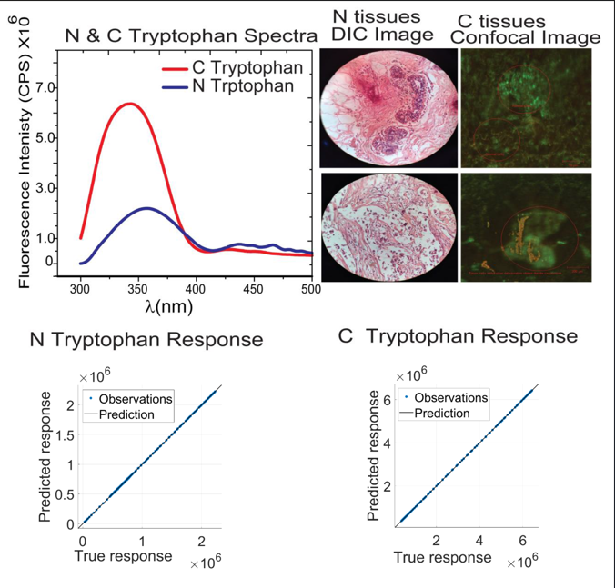
In the case of tryptophan spectra, blood serum of normal and cancerous patients excited at 280 nm and fluorescence spectra acquired on fluorescence spectrometer keeping collection range from 300-500 nm while in the case of NADH blood serum of corresponding patients excited at 340 nm and fluorescence spectra acquired on fluorescence spectrometer keeping collection range from 375-600 nm. In the case of FAD, blood serum of normal and cancerous patients was excited at 360 nm and fluorescence spectra were acquired on the fluorescence spectrometer, keeping the collection range from 440-640 nm. The obtained spectra are shown in Figure 2.
It is much more important to diagnose BC at the micro level using fluorescence spectral properties. Instead, physical models approach the cost of the patient’s health. Standard BC screening techniques did not work to detect small and asymmetrical-shaped tumors in condensed breast tissues. Realistically, tumor models are used, which make use of absorption, diffuse scattering, and fluorescence properties simultaneously to tackle and diagnose tissues. When biological samples are excited with light of a suitable wavelength (), it results in the emission of light with a longer [41]. The collection and analysis of auto-fluorescence signals from tissues is useful for the development of instruments and devices for disease diagnosis and screening. Endogenous fluorophores (tryptophan, NADH, and FAD) have an important role in the metabolism of living cells and tissues [42]. Normal, benign, and malignant tissues differ in their metabolic activity, so the concentration and, consequently auto-fluorescence intensity of these endogenous fluorophores vary in respective tissues and are used to differentiate normal and aggressive cells. These key intrinsic fluorophores in cells and tissues exhibit specific spectrum signatures for absorption and emission from UV-VIS. Being the turbid nature of these tissues, it is difficult to differentiate on the basis of absorption spectroscopy alone.
Tryptophan is identified as a fingerprint for identifying aggressiveness among BC cell line [43]. Tryptophan converts to serotonin within the brain. The serotonin system is vital in the endocrine regulation of reproductive hormone production, and it may alter gonadotropin-releasing hormone (GnRH) pulsatility, which is necessary for reproductive processes [44]. So, the effect appears in the form of aggressiveness to females and is used for BC diagnosis. Müller et al. [45] used a photon migration model to extract the intrinsic fluorescence from the tissue fluorescence measured from the human oral cavity. They found that the displayed intrinsic fluorescence greatly reduced variability in intensity and line shape compared to the turbid tissue fluorescence. Coenzymes NADPH and NADH are two prominent fluorophores responsible for the shape of the fluorescence spectrum of the breast tissue and other tissue types. These coenzymes play a vital role in a metabolic oxidation-reduction process and are also correlated with the redox ratio.
The differentiated spectra of normal and blood serum ultimately guided us toward the development of an integrating sphere light source that can be used to differentiate normal and cancer patients’ serum on the basis of endogenous fluorophores like tryptophan, NADH, and FAD. These auto-fluorescence spectra will provide the basis for the diagnosis of BC at an early stage and provide a route of information for the design and development of BC screening devices. The emission spectrum of NADH measured at 340 nm excitation shows no statistically significant differences (ES) in fluorescent response of tissues. The changes in the metabolic status of tissue obviously have influence on the variation in concentrations of both the coenzymes. It has been established that in a high-grade malignant tissue appear increased levels of these coenzymes [46].
There is always an existence of intra-variance in the spectra of individuals who are different from each other due to Patho-biochemical, and further explanation is still unclear. However, on a molecular level, it has been found that serum amino acid, especially intrinsic auto-fluorescence, is responsible for this type of behavior [47]. The fluorescence quantum yield of tryptophan is 0.13 [48], which is the proportion of photons emitted to absorbed one [37]. Figure 2(a) describes that tryptophan shows aggressiveness towards BC. The high fluorescence intensity of tryptophan was found in cancer serum as compared to normal serum. This type of fingerprint was found to be for normal and cancer breast cell lines also [37].
3.2. Confocal and DIC imaging
H&E stained images provide important information about the structure, pattern, and shape of tissue and cells under investigation. DIC images of both normal and cancerous stained slides were acquired. H&E images of both normal and cancerous breast tissues are shown in Figure 3(a) through (f). DIC images in Figure 3(a) through (c) have regular structures with all types of cells, while in the case of Figure 3(d) through (f), cancer cells have lost their regular structures. H&E staining is a standard histological technique that provides detailed information about the cellular structure and organization of tissues. It allows pathologists to visualize various cell types, nuclei, and other structures within the tissue sample. It can reveal metabolic and structural changes.
Confocal auto-fluorescence imaging is a technique used to examine the intrinsic fluorescence properties of tissues without the need for external labelling. In the context of BC, it can help to differentiate between normal and cancerous tissues based on their auto-fluorescence properties. It can produce images of human breast tissues of normal and cancerous breast cells [48]. Intrinsic fluorophores inside the cells give fluorescence after the excitation on appropriate wavelengths. A confocal microscope in reflectance mode and spectral information confocal images are used for margin assessment during post-operative for breast subcellular resolution and margin marking status [49]. It provides a tool that can be used to depict adipocyte morphology and other features of the tumor microenvironment located adjacent to and far from ductal carcinoma [50]. Cancerous tissues often exhibit alterations in cellular metabolism and composition, manifesting as changes in auto-fluorescence compared to normal tissues. Confocal images are superior to conventional histopathological images because they are real-time, high resolution, and produced by fluorescence after proper excitation. Confocal fluorescence images at different magnifications produced using the cancerous samples are shown in Figure 4(a) through (c). When comparing confocal auto-fluorescence imaging with H&E-stained DIC images, scientists can gather complementary information about tissue morphology and composition. Images acquired on a confocal microscope differentiate normal and malignant cells in tissue slides.
3.3. Regression Performance Analysis of BC Detection
The metabolic activity of cells can be measured indirectly by varying endogenous fluorophores, viz., tryptophan enzymes and their coenzymes. In this study, the optical diagnosis of BC has been carried out on fluorescence spectra of fluorophore tryptophan, NADH, and FAD for healthy and diseased subjects using their confocal images. The emission intensity of biomarker tryptophan in the cancerous (C-tryptophan) serum is (4-8 million counts at FWHM) as compared with the normal blood samples (N-tryptophan) with intensity of 1.50-2.75 million counts at FWHM. The objective of this regression analysis is to predict BC in unknown samples by correlating their response variables with either cancerous or healthy profiles. The regression model estimates approximate emission spectrum values for C- and N-tryptophan, highlighting predicted counts. To further validate and confirm the diagnosis of BC, additional regression analyses of C-NADH and C-FAD are performed. This predictive information can serve as a valuable supplementary tool for clinicians, trainees, and medical experts in treatment planning and accurate diagnosis of BC.
3.3.1. C- and N- tryptophan
The experimentations for different regression-based ML models have been conducted using open source libraries along with standard programming environments and tools using a Dell G7 laptop (Intel ® CoreTM 8th Generation CPU) using 32 GB RAM and 6 GB GPU (NVIDIA GTX-1060 with 1280 CUDA cores). The dataset of 300 patients (Section 2.1) is cross validated 10-fold for five potential regression models.
The experimentation was initiated by selecting an appropriate parametric set. Table 2 presents a sensitivity analysis of regression parameters, validated through 10-fold cross-validation using five potential regression models. Each model was carefully configured to optimize its predictive capability by tuning key parameters.
The GPR model was configured with a constant basis function and a Matern 5/2 kernel function. An isotropic kernel was used, which assumes uniform properties in all directions. Several hyperparameters, including the kernel scale, signal standard deviation, and sigma, were set to be automatically determined during training. Additionally, numeric parameters were optimized to improve the model's accuracy and robustness. Model 2, the WNN, was constructed with a single fully connected layer comprising 100 neurons. The ReLU activation function was applied to introduce non-linearity, and training was capped at 1000 iterations to balance performance with computational efficiency. No regularization was applied, as the lambda value was set to zero, and the input data was standardized to ensure consistent feature scaling across the network. The SVR utilized a Gaussian kernel with a fixed kernel scale of 1. The model's box constraint and epsilon parameters were automatically optimized during training. Similar to the WNN, the SVR model also included data standardization to enhance model convergence and performance. The FDT was designed with a minimum leaf size of 4, enabling the tree to capture fine-grained patterns in the data. To maintain a straightforward structure and avoid additional computational complexity, surrogate decision splits were turned off. The BT consisted of 30 learners and a minimum leaf size of 8. A learning rate of 0.1 was chosen to moderate the contribution of each tree in the ensemble, striking a balance between learning speed and model generalization.
The mean value for each set of tryptophan, NADH, and FAD data concerning the cancerous and healthy subjects have been used for cross-validation analysis. In this study, as illustrated in Table 3, C-Tryptophan fluorescence intensity was investigated as a non-invasive biomarker for breast cancer detection, integrated for the first time with GPR and validated through confocal and histopathological imaging. The regression models were evaluated using a 10-fold cross-validation approach, with fluorescence intensity values standardized across a range of 6 × 10⁶. Among the tested models, GPR, WNN, SVR, FDT, and BT, GPR demonstrated superior performance in both validation and testing phases. It achieved the lowest validation RMSE (3406.5) and MAE (2387.2), alongside a perfect R² score of 1.00, indicating an ideal correlation between predicted and actual values. Testing metrics further confirmed GPR’s robustness, with an RMSE of 3621.6 and MAE of 2573.2, again supported by an R² of 1.00. Additionally, GPR maintained a fast training time of 1.123 seconds, emphasizing its computational efficiency.
In contrast, the WNN model, despite a high R², exhibited significantly higher RMSE (19140.0) and training time (6.667 seconds), suggesting overfitting and poor generalizability. SVR, FDT, and BT showed moderately good performance but fell short in matching the prediction accuracy and consistency offered by GPR. These findings underscore the ability of GPR to model nonlinear and complex biochemical patterns such as serum tryptophan fluorescence, providing a high-fidelity predictive framework suitable for biomedical applications.
The fluorescence of N-Tryptophan, as shown in Table 4, was investigated as a biomarker for modeling N-tryptophan metabolism, employing regression-based ML methods to evaluate predictive performance. This represents the first application of serum N-Tryptophan fluorescence integrated with GPR and validated using confocal and histopathological imaging in the context of breast cancer diagnostics. A 10-fold cross-validation was conducted using five different regressors, GPR, WNN, SVR, FDT, and BT models, on fluorescence intensity data ranging up to 2 × 10⁶.
Among all models, GPR demonstrated outstanding performance in both validation and testing phases. It yielded the lowest validation RMSE (2195.9) and MAE (1585.8), with a perfect R² score of 1.00 and minimal training time of 0.962 seconds. On the test dataset, GPR again outperformed all other models with a testing RMSE of 1847.5, an R² of 1.00, and a MAE of 1391.9, showcasing its remarkable ability to accurately generalize across unseen data. These results emphasize GPR’s ability to capture the subtle spectral nuances of tryptophan fluorescence in healthy individuals, making it a robust tool for distinguishing normal metabolic states.
In contrast, the WNN, while demonstrating reasonable accuracy (testing R² = 0.99), had a significantly higher RMSE (12750.0) and MAE (10210.0), coupled with a longer training time (6.157 seconds), indicating reduced efficiency and greater computational cost. Other models, including SVR, FDT, and BT, showed significantly higher error values, particularly with SVR and FDT reaching MAEs of 58426.0 and 40551.0, respectively, highlighting their limitations in modeling complex biochemical fluorescence data.
Figure 5 presents visual analysis of the results of GPR-model applied to the fluorescence spectra of cancerous and normal tryptophan samples. The top row, Figure 5(a) through (d), corresponds to cancerous tryptophan (C-tryptophan), while the bottom row, Figure 5(e) through (h), illustrates the analysis for normal tryptophan (N-tryptophan). Figure 5(a)&(e) show the actual fluorescence intensity data for C- and N-tryptophan, respectively, whereas Figure 5(b)&(f) display the predicted spectra obtained using the GPR model. The corresponding prediction errors, calculated as the difference between the actual and predicted values, are illustrated in Figure 5(c) for C-tryptophan and Figure 5(g) for N-tryptophan. To provide a comprehensive visualization of model performance, Figure 5(d)&(h) merge the actual, predicted, and error data for both cancerous and normal samples.
The x-axis in all plots represents the wavelength (λ) in nanometers (nm), while the y-axis denotes fluorescence intensity in arbitrary units (a.u.). The visual comparison between the actual and predicted curves demonstrates that the GPR model accurately captures the spectral patterns of both sample types, with minimal discrepancies highlighted in the error plots. These findings indicate the potential of GPR as a reliable regression model for fluorescence-based biomarker analysis, especially in distinguishing between normal and cancerous biological state.
Figure 6 presents a comparative evaluation of models other than GPR applied to cancerous (C-tryptophan) and normal (N-tryptophan) fluorescence data. Figure 6(a) through (d) display the actual versus predicted fluorescence spectra, along with associated errors, for C-tryptophan using Models 2, 3, 4, and 5, respectively. The same sequence of models for N-tryptophan is shown in Figure 6€ through (h). These plots illustrate how each model captures the fluorescence intensity trends (in arbitrary units) across the wavelength range of 300–500 nm. The close alignment between the actual and predicted curves, along with minimal error bands, suggests a strong predictive capability of the models.
To further evaluate the prediction accuracy of the GPR models, Predicted vs. Actual (PvA) plots are presented in Figure 6(i) through (l). Figure 6(i) shows the PvA plot for C-tryptophan using the GPR model, while Figure 6(k) presents the same for N-tryptophan. These plots reflect how closely the predicted fluorescence intensities of GPR align with the true responses. Figure 6(j)&(l) display the PvA plots specifically for Model 5 applied to C-tryptophan and N-tryptophan, respectively. In the case of GPR, the predicted responses closely align with the true values, as indicated by the clustering of points around the ideal diagonal line. These results underscore the potential of model-based spectral analysis for distinguishing between cancerous and normal tryptophan signatures with high precision.
3.3.2. C- and N-NADH
In this study, C-NADH fluorescence data were analyzed as a potential metabolic biomarker for breast cancer detection, utilizing ML regression models validated by confocal and histopathological imaging, as presented in Table 5. This represents the first known integration of serum C-NADH fluorescence with GPR for cancer detection. Using a 10-fold cross-validation strategy, five regression models, GPR, WNN, SVR, FDT, and BT, were assessed for their ability to predict C-NADH intensity values within a fluorescence range of 11 × 10⁶.
Among all models tested, GPR demonstrated superior accuracy, consistency, and efficiency. It yielded the lowest validation RMSE (10776.0) and MAE (6036.5) with an R² of 1.00, indicating an almost perfect fit to the training data. GPR also exhibited efficient computation with a short training time of 0.986 seconds. In testing, GPR again delivered the best performance, with a testing RMSE of 10139.0, R² of 1.00, and MAE of 6791.4, outperforming all other regressors. These results affirm GPR’s reliability in modeling the spectral variations associated with elevated NADH concentrations observed in cancerous tissues.
In contrast, the WNN model, despite a similar R² value, presented far higher RMSE (72781.0) and MAE (52601.0) values in the test set, suggesting that while it could capture general trends, it lacked the precision and stability offered by GPR. Similarly, SVR, FDT, and BT exhibited greater predictive errors, with testing MAE values ranging from 21041.0 to 24052.0, confirming their limitations in handling the non-linear spectral complexity of C-NADH signals.
In another experiment, N-NADH fluorescence intensity was examined as a biomarker of normal metabolic states, with predictive modeling performed using advanced regression algorithms, as demonstrated in Table 6. The dataset was subjected to 10-fold cross-validation, and the fluorescence intensity range for N-NADH was set at 6 × 10⁶. Among the five regression models assessed, GPR, WNN, SVR, FDT, and BT, GPR again emerged as the most effective model in capturing the spectral characteristics of N-NADH.
GPR achieved the lowest validation RMSE of 6866.4 and MAE of 3959.8, alongside a perfect R² of 1.00, indicating an exceptional fit. Its performance remained consistent during testing, where it recorded an RMSE of 4917.6, a testing MAE of 3683.8, and an R² of 1.00. These metrics underscore GPR’s high precision and reliability in modeling normal NADH profiles. Furthermore, GPR maintained computational efficiency with a short training time of 1.125 seconds, making it both accurate and resource-effective.
In contrast, the WNN model exhibited significantly higher error rates, with a testing RMSE of 54425.0 and MAE of 48054.0, despite its moderate training R² of 0.90. SVR and tree-based models (FDT and BT) performed better than WNN in terms of correlation (R² > 0.98), but still lagged behind GPR in RMSE and MAE values. Notably, their MAEs ranged from 17502.0 to 31002.0, highlighting less stable prediction capacity across N-NADH intensity values.
Figure 7 illustrates the visual aspects of GPR model applied to the fluorescence spectra of C- and N- NADH samples. The top row, Figure 7(a) through (d) represents the results for C-NADH, while the bottom row, Figure 7(e) through (h) corresponds to N-NADH. Figure 7(a)&(e) display the actual fluorescence intensity spectra, and Figure 7(b)&(f) show the predicted spectra generated by the GPR model for cancerous and normal samples, respectively. The prediction errors, calculated as the difference between the actual and predicted values, are shown in Figure 7(c)&(g).
To provide a comprehensive assessment, Figure 7(d)&(h) present a merged view of actual, predicted, and error data for C- and N-NADH, respectively. Across all plots, the x-axis represents the wavelength (λ) in nanometers (nm), and the y-axis shows fluorescence intensity in arbitrary units (a.u.). The visual alignment between the actual and predicted curves, along with minimal deviation in the error plots, indicates that the GPR model is capable of accurately capturing the spectral behavior of C- and N-NADH samples.
Figure 8 presents the comparative performance evaluation of models other than GPR, Models 2-5, applied to C- and N-NADH fluorescence data. Figure 8(a) through (d) show the results for C-NADH using Models 2, 3, 4, and 5, respectively. Similarly, Figure 8(e) through (h) display the corresponding model outputs for N-NADH. Each of these plots compares the actual and predicted fluorescence intensity spectra, along with the associated prediction error, across the wavelength range of 350–600 nm. The close alignment between actual and predicted curves, accompanied by narrow error bands, suggests that the models effectively capture the underlying spectral characteristics.
To assess the model accuracy quantitatively, PvA plots are shown in Figure 8(i) through (l). Figure 8(i)&(k) present the overall PvA comparisons using the GPR model for C- and N-NADH, respectively. Figure 8(j)&(l) illustrate the PvA plots specifically for Model 5 applied to C- and N-NADH. In Figure 8(i)&(k) plots, data points lie close to the diagonal line, indicating a high level of agreement between predicted and actual responses. These findings confirm the strong predictive capability and generalizability of the GPR model in analyzing NADH fluorescence signatures in both cancerous and normal conditions.
3.3.3. C- and N-FAD
C-FAD fluorescence intensity was analyzed as a potential metabolic biomarker for breast cancer detection, as shown in Table 7. The research integrates spectral data with advanced ML regressors and validates outcomes through confocal and histopathological imaging, marking the first known use of GPR in modeling C-FAD fluorescence for oncological diagnostics. Five regression algorithms, GPR, WNN, SVR, FDT, and BT, were assessed under a 10-fold cross-validation framework using a fluorescence intensity range of 7.5 × 10⁶.
GPR consistently outperformed all other models, delivering the best predictive performance across both validation and testing datasets. In the validation phase, GPR achieved a low RMSE of 6776.0 and MAE of 6237.6, along with a perfect R² value of 1.00, indicating near-ideal model fit. On the test data, GPR again demonstrated excellent generalization capacity, with an RMSE of 5858.5 and MAE of 4065.9, substantially outperforming competing models. Its training time was also efficient at 0.862 seconds, confirming GPR’s capability to balance both accuracy and computational economy.
In contrast, the WNN model, while yielding a high R² of 1.00, showed much higher error metrics, with a testing RMSE of 9404.9 and MAE of 7479.8. SVR and FDT, despite moderately high correlation scores (R² between 0.94 and 0.95), exhibited larger prediction errors and lower robustness. The BT model showed the weakest performance with an R² of only 0.683 and a testing MAE of 32045.0, rendering it unsuitable for precise clinical prediction.
The fluorescence intensity of N-FAD was modeled using ML algorithms to establish a metabolic baseline in healthy individuals, as illustrated in Table 8.This work marks the integration of serum tryptophan and coenzyme fluorescence data with GPR, supported by confocal and histopathological imaging for validation. A total of five regression models, GPR, WNN, SVR, FDT, and BT, were employed to evaluate predictive performance using 10-fold cross-validation across a fluorescence intensity range of 5 × 10⁶.
GPR emerged as the most accurate and reliable regressor, demonstrating exceptional results in both training and testing phases. During validation, GPR recorded a minimal RMSE of 3207.0 and MAE of 3188.4, accompanied by a perfect R² value of 1.00. This performance extended to the test set, where GPR achieved the lowest RMSE (2819.5) and MAE (2444.6), again with a flawless R² of 1.00, confirming its ability to generalize effectively to unseen data. Moreover, GPR achieved these results with a rapid training time of just 1.008 seconds, reflecting its computational efficiency.
In comparison, the WNN model, while maintaining a high R² of 1.00, presented much larger errors (test RMSE: 12,109.0; MAE: 9177.2), suggesting overfitting or limited robustness. Other regressors, including SVR, FDT, and BT, showed moderate predictive accuracy (R²: 0.95–0.98), but with significantly higher error metrics. The BT model, in particular, underperformed with an R² of 0.93 and MAE exceeding 67678.0, indicating its unsuitability for precise metabolic profiling.
In this study, all these findings underscore the suitability of GPR for modeling normal FAD fluorescence patterns, enabling accurate characterization of normal metabolic states. This method provides a reliable baseline for differentiating between healthy and pathological conditions. The high fidelity of GPR-based predictions supports its application in non-invasive diagnostics, facilitating early detection strategies through comparative metabolic fluorescence mapping in clinical oncology.
Figure 9 illustrates visual analysis of the application of GPR to the fluorescence spectra of C- and N-FAD samples. The top row, Figure 9(a) through (d), represents the results for C-FAD, while the bottom row, Figure 9(e) through (h), displays the results for N-FAD. Specifically, Figure 9(a)&(e) show the actual fluorescence intensity data, and Figure 9(b)&(f) present the predicted spectra generated by the GPR model. The prediction errors, calculated as the difference between the actual and predicted values, are shown in Figure 9(c)&(g) for cancerous and normal samples, respectively.
Figure 9(d)&(h) provide merged views of the actual, predicted, and error data for C- and N-FAD, respectively. The x-axis in all plots represents the wavelength (λ) in nanometers, and the y-axis indicates fluorescence intensity in arbitrary units (a.u.). The close alignment between the predicted and actual data, with minimal error deviation, demonstrates the strong predictive accuracy of the GPR model. These results highlight the potential of GPR in modeling fluorescence behavior and distinguishing between cancerous and non-cancerous biochemical states using FAD spectral information.
Figure 10 presents the comparative performance of GPR model applied to the fluorescence spectra of C- and N-FAD samples. Figure 10 (a) through (d) show the GPR results for C-FAD using Models 2, 3, 4, and 5, respectively, while Figure 10 (e) through (h) display the corresponding results for N-FAD. Each plot includes actual and predicted fluorescence intensity curves along with associated prediction errors, allowing for visual assessment of model accuracy across the spectral range of 450–600 nm. The close overlap between actual and predicted data across GPR reflects its capacity to accurately replicate spectral patterns in cancerous and normal conditions.
To further assess model performance, PvA plots are shown in Figure 10(i) through (l). Figure 10(i) displays the overall PvA comparison for C-FAD using the GPR model, while Figure 10(k) presents the same for N-FAD. Figure 10(j)&(l) highlight PvA plots specifically for Model 5 applied to C- and N-FAD, respectively. In the case of GPR, the data points closely align with the ideal diagonal line, confirming the strong predictive accuracy. These results underscore the robustness of GPR models in capturing and distinguishing the fluorescence behavior of C- and N-FAD.
3.4. Main Findings of Regression Analysis
The theme of this study is the early diagnosis of BC to enhance the retrieval rate. In this context, the optical techniques are highly encouraging with no side effects and there is no need of any labelling. The fluorophores biomolecules, namely tryptophan, NADH, and FAD, are actively involved in the metabolic events of cells. The variation of these biomolecules’ concentration in the tumorous region has been found helpful in tracking metabolic activities and a difference in fluorescence properties of normal and cancerous breast tissues.
The emission intensity of tryptophan (biomarker) in the cancerous serum samples is different from the normal blood sera (normal serum: 1.5-2.75 million counts at FWHM and malignant serum: 4.0-8.0 million counts at FWHM) after excitation at 280±5 nm. This noteworthy difference in counts has been analyzed using ML techniques through regression-based prediction and validation study of tryptophan (normal/ cancerous cases) using GPR, WNN, SVR, FDT, and BT models. The potential performance measures include RMSE, R-squared, MSE, and MAE. Based on this dual-phase study's practical and theoretical results with intensive data collection, we suggest a portable optical screening device for the medical community.
Statistical analysis confirms significant differences in fluorescent characteristics of normal and malignant breast tissue in the whole emission range to distinguish early-stage and advanced-stage BC with reasonable sensitivity and specificity [49]. It is possible to perceive the endogenous auto-fluorescence from coenzymes, including NADH and FAD, important biomolecules that are involved in key metabolic pathways such as oxidative phosphorylation, glycolysis, and Krebs cycle. Among the investigated fluorophores, tryptophan emerged as a particularly strong biomarker for early breast cancer detection. Together, the distinct fluorescence profiles of tryptophan, NADH, and FAD provide a solid foundation for non-invasive diagnostic approaches. Future research combining these spectral biomarkers with advanced techniques like DL may further improve diagnostic accuracy and efficiency.
4. Conclusions and Future Work
Optical techniques offer early diagnosis of BC without any side effects to humans. Endogenous fluorophores such as tryptophan, enzymes, and their coenzymes NADH and FAD play a vital part in the metabolic activities of cells. The varying concentration of these biomolecules throughout the tumor determines their metabolic activities. Normal and cancerous patients on the basis of tryptophan fluorescence spectra are the main subjects of this study. NADH and FAD intrinsic fluorescence spectra and confocal images were studied to validate the authenticity of this optical differentiation. The higher emission intensity of tryptophan biomarkers in the cancerous serum is the dominant parameter of differentiation as compared to normal blood sera. In the case of normal serum samples, it varies from 1.5-2.75 million counts at FWHM, while in the case of malignant blood sera, it varies from 4.0-8.0 million counts at FWHM after excitation at 280±5 nm, i.e., a clear and evident difference. The sensitivity analysis of tryptophan, NADH, and FAD for normal and cancerous patients has been found encouraging using regression ML through GPR, WNN, SVR, FDT, and BT models. All the study will guide us to produce a fluorescence BC screening device fused with a ML method.
Author Contributions
Conceptualization, Aziz-ul- Rehman and Shahzad Ahmad Qureshi; Methodology, Aziz-ul- Rehman, Shahzad Ahmad Qureshi, Hamna Azhar, Uzma Ghazanfar, Asma Khattak and Babar Manzoor Atta Babar Manzoor Atta; Software, Shahzad Ahmad Qureshi and Qurat-ul-ain Aslam; Validation, Aziz-ul- Rehman, Shahzad Ahmad Qureshi, Qurat-ul-ain Aslam, Asma Khattak and Babar Manzoor Atta Babar Manzoor Atta; Formal analysis, Aziz-ul- Rehman, Shahzad Ahmad Qureshi, Hamna Azhar, Qurat-ul-ain Aslam and Uzma Ghazanfar; Investigation, Aziz-ul- Rehman, Hamna Azhar and Babar Manzoor Atta Babar Manzoor Atta; Resources, Shahzad Ahmad Qureshi; Data curation, Shahzad Ahmad Qureshi and Babar Manzoor Atta Babar Manzoor Atta; Writing – original draft, Aziz-ul- Rehman, Hamna Azhar, Qurat-ul-ain Aslam, Uzma Ghazanfar and Babar Manzoor Atta Babar Manzoor Atta; Writing – review & editing, Aziz-ul- Rehman, Shahzad Ahmad Qureshi, Asma Khattak and Babar Manzoor Atta Babar Manzoor Atta; Visualization, Aziz-ul- Rehman, Shahzad Ahmad Qureshi and Uzma Ghazanfar. All authors have read and agreed to the published version of the manuscript.
Institutional Review Board Statement
The samples slides of confirmed BC patients and normal subjects used in this study were taken from the Pakistan Institute of Medical Sciences (PIMS), Islamabad, and the Pakistan Atomic Energy Commission (PAEC) General Hospital, Nilore, Islamabad, in December 2023 after ethical and legal permissions.
Data Availability Statement
The data presented in this study are available on request from the corresponding author.
Conflicts of Interest
The authors declare no conflict of interest.
References
- Bray, F.; et al. Cancer Incidence in Five Continents: inclusion criteria, highlights from Volume X and the global status of cancer registration. International journal of cancer 2015, 137, 2060–2071. [Google Scholar] [CrossRef] [PubMed]
- Sung, H.; et al. Global cancer statistics 2020: GLOBOCAN estimates of incidence and mortality worldwide for 36 cancers in 185 countries. CA: a cancer journal for clinicians 2021, 71, 209-249.
- Li, J.; et al. Non-invasive biomarkers for early detection of breast cancer. Cancers 2020, 12, 2767. [Google Scholar] [CrossRef] [PubMed]
- Chung, H.W.; et al. PET/MRI and Novel Targets for Breast Cancer. Biomedicines 2024, 12, 172. [Google Scholar] [CrossRef] [PubMed]
- Aymaz, S. , A new framework for early diagnosis of breast cancer using mammography images. Neural Computing and Applications 2024, 36, 1665–1680. [Google Scholar] [CrossRef]
- Li, H., J. Zhao, and Z. Jiang, Deep learning based computer-aided detection of ultrasound in breast cancer diagnosis: a systematic review and meta-analysis. Clinical Radiology, 2024.
- Morrow, M. and S. Schnitt, Ductal carcinoma in situ and microinvasive carcinoma. Diseases of the Breast 2nd edition. Harris JR, Lippman ME, Morrow M, Osborne CK eds. 2000, Lippincott Williams & Wilkins. Philadelphia.
- Obeagu, E.I.; Obeagu, G.U. Breast cancer: A review of risk factors and diagnosis. Medicine 2024, 103, e36905. [Google Scholar] [CrossRef] [PubMed]
- Tian, X.; et al. Application of Raman spectroscopy technology based on deep learning algorithm in the rapid diagnosis of glioma. Journal of Raman Spectroscopy 2022, 53, 735–745. [Google Scholar] [CrossRef]
- Qureshi, S.A.; et al. Breast Cancer Detection using Mammography: Image Processing to Deep Learning. IEEE Access, 2024.
- Dramićanin, T., M. Dramićanin, and M. Stauffer, Using fluorescence spectroscopy to diagnose breast cancer. Appl Mol Spectrosc to Curr Res Chem Biol Sci, 2016.
- Kim, H.J.; et al. High-resolution diffusion-weighted MRI plus mammography for detecting clinically occult breast cancers in women with dense breasts. European Journal of Radiology, 2024. 175: p. 111440.
- Choi, S.; et al. A multi-institutional analysis of factors influencing the rate of positive MRI biopsy among women with early-stage breast cancer. Annals of surgical oncology 2024, 31, 3141–3153. [Google Scholar] [CrossRef] [PubMed]
- Ma, M.; et al. Advances in the clinical application of Raman spectroscopy in breast cancer. Applied Spectroscopy Reviews, 2024: p. 1-35.
- Gayen, S.; Alfano, R. Emerging optical biomedical imaging techniques. Optics and Photonics news 1996, 7, 16. [Google Scholar] [CrossRef]
- Vishwanath, K. and N. Ramanujam, Fluorescence spectroscopy in vivo. Encyclopedia of Analytical Chemistry: Applications, Theory and Instrumentation, 2006.
- Dramićanin, T.; et al. Biophysical characterization of human breast tissues by photoluminescence excitation-emission spectroscopy. Journal of Research in Physics 2012, 36, 53–62. [Google Scholar] [CrossRef]
- Maroof, N.; et al. Mitosis detection in breast cancer histopathology images using hybrid feature space. Photodiagnosis and photodynamic therapy, 2020. 31: p. 101885.
- Chen, H., X. Wang, and P.A. Heng. Automated mitosis detection with deep regression networks. in 2016 IEEE 13th International Symposium on Biomedical Imaging (ISBI). 2016. IEEE.
- Alsayadi, H.A.; et al. Ensemble of Machine Learning Fusion Models for Breast Cancer Detection Based on the Regression Model. Fusion: Practice & Applications, 2022. 9(2).
- Mihaylov, I., M. Nisheva, and D. Vassilev, Application of machine learning models for survival prognosis in breast cancer studies. Information 2019, 10, 93.
- Deringer, V.L.; et al. Gaussian process regression for materials and molecules. Chemical Reviews 2021, 121, 10073–10141. [Google Scholar] [CrossRef] [PubMed]
- Schulz, E., M. Speekenbrink, and A. Krause, A tutorial on Gaussian process regression: Modelling, exploring, and exploiting functions. Journal of Mathematical Psychology, 2018. 85: p. 1-16.
- Canatar, A., B. Bordelon, and C. Pehlevan, Spectral bias and task-model alignment explain generalization in kernel regression and infinitely wide neural networks. Nature communications 2021, 12, 2914.
- Drucker, H.; et al. Support vector regression machines. Advances in neural information processing systems, 1996. 9.
- Cortes, C. and V. Vapnik, Support-Vector Networks. Machine Learning, 1995.
- Gonzalez-Navarro, F.F.; et al. Glucose oxidase biosensor modeling and predictors optimization by machine learning methods. Sensors 2016, 16, 1483. [Google Scholar] [CrossRef] [PubMed]
- Ni, K.S. and T.Q. Nguyen, Image superresolution using support vector regression. IEEE Transactions on Image Processing. 2007; 16, 1596–1610.
- Cui, F.; et al. Advancing biosensors with machine learning. ACS sensors 2020, 5, 3346–3364. [Google Scholar] [CrossRef] [PubMed]
- AKINCI, T.Ç. and H.S. NOĞAY, Application of decision tree methods for wind speed estimation. European Journal of Technique (EJT) 2019, 9, 74–83. [Google Scholar] [CrossRef]
- De'Ath, G. Boosted trees for ecological modeling and prediction. Ecology 2007, 88, 243–251. [Google Scholar] [CrossRef] [PubMed]
- Elith, J., J. R. Leathwick, and T. Hastie, A working guide to boosted regression trees. Journal of animal ecology 2008, 77, 802-813.
- Plevris, V., et al. Investigation of performance metrics in regression analysis and machine learning-based prediction models. in 8th European Congress on Computational Methods in Applied Sciences and Engineering (ECCOMAS Congress 2022). 2022. European Community on Computational Methods in Applied Sciences.
- Khan, M. and S. Noor, Performance analysis of regression-machine learning algorithms for predication of runoff time. Agrotechnology 2019, 8, 1-12.
- Chicco, D., M. J. Warrens, and G. Jurman, The coefficient of determination R-squared is more informative than SMAPE, MAE, MAPE, MSE and RMSE in regression analysis evaluation. PeerJ Computer Science, 2021. 7: p. e623.
- Botchkarev, A. , Performance metrics (error measures) in machine learning regression, forecasting and prognostics: Properties and typology. arXiv:1809.03006, 2018.
- Lakowicz, J.R. Principles of Fluorescence Spectroscopy. 2013. 954.
- Vishwanath, K. and M.-A. Mycek, Do fluorescence decays remitted from tissues accurately reflect intrinsic fluorophore lifetimes? Optics letters 2004, 29, 1512-1514.
- Kotaki, A. and K. YAGI, Fluorescence properties of flavins in various solvents. The Journal of Biochemistry 1970, 68, 509-516.
- Macheroux, P., S. Chapman, and G. Reid, Flavoprotein protocols. Methods in Molecular Biology, 1999. 131: p. 1-7.
- Rehman, A.U.; et al. Fluorescence quenching of free and bound NADH in HeLa cells determined by hyperspectral imaging and unmixing of cell autofluorescence. Biomed Opt Express 2017, 8, 1488–1498. [Google Scholar] [CrossRef] [PubMed]
- Georgakoudi, I. and K.P. Quinn, Optical imaging using endogenous contrast to assess metabolic state. Annual review of biomedical engineering, 2012. 14: p. 351-367.
- Zhang, L.; et al. Tryptophan as the fingerprint for distinguishing aggressiveness among breast cancer cell lines using native fluorescence spectroscopy. Journal of biomedical optics 2014, 19, 037005. [Google Scholar] [CrossRef] [PubMed]
- Comai, S.; et al. Serum levels of tryptophan, 5-hydroxytryptophan and serotonin in patients affected with different forms of amenorrhea. International Journal of Tryptophan Research, 2010. 3: p. IJTR. S3804.
- Müller, M.G.; et al. Intrinsic fluorescence spectroscopy in turbid media: disentangling effects of scattering and absorption. Applied Optics 2001, 40, 4633–4646. [Google Scholar] [CrossRef] [PubMed]
- Georgakoudi, I.; et al. NAD (P) H and collagen as in vivo quantitative fluorescent biomarkers of epithelial precancerous changes. Cancer research 2002, 62, 682–687. [Google Scholar] [PubMed]
- Hubmann, M.R., M. Leiner, and R.J. Schaur, Ultraviolet fluorescence of human sera: I. Sources of characteristic differences in the ultraviolet fluorescence spectra of sera from normal and cancer-bearing humans. Clinical chemistry 1990, 36, 1880-1883.
- Chen, R.F. , Fluorescence quantum yields of tryptophan and tyrosine. Analytical Letters 1967, 1, 35–42. [Google Scholar] [CrossRef]
- Kalaivani, R.; et al. Fluorescence spectra of blood components for breast cancer diagnosis. Photomedicine and Laser Surgery 2008, 26, 251–256. [Google Scholar] [CrossRef] [PubMed]
Figure 1.
(a) Tryptophan EEM spectrum, and (b) Peak auto-fluorescence intensity of 0.5 M tryptophan solution measured using Horiba FluoroMax 4 Spectrofluorometer showed a peak at 380±5 nm when excited at 280±5 nm.
Figure 1.
(a) Tryptophan EEM spectrum, and (b) Peak auto-fluorescence intensity of 0.5 M tryptophan solution measured using Horiba FluoroMax 4 Spectrofluorometer showed a peak at 380±5 nm when excited at 280±5 nm.
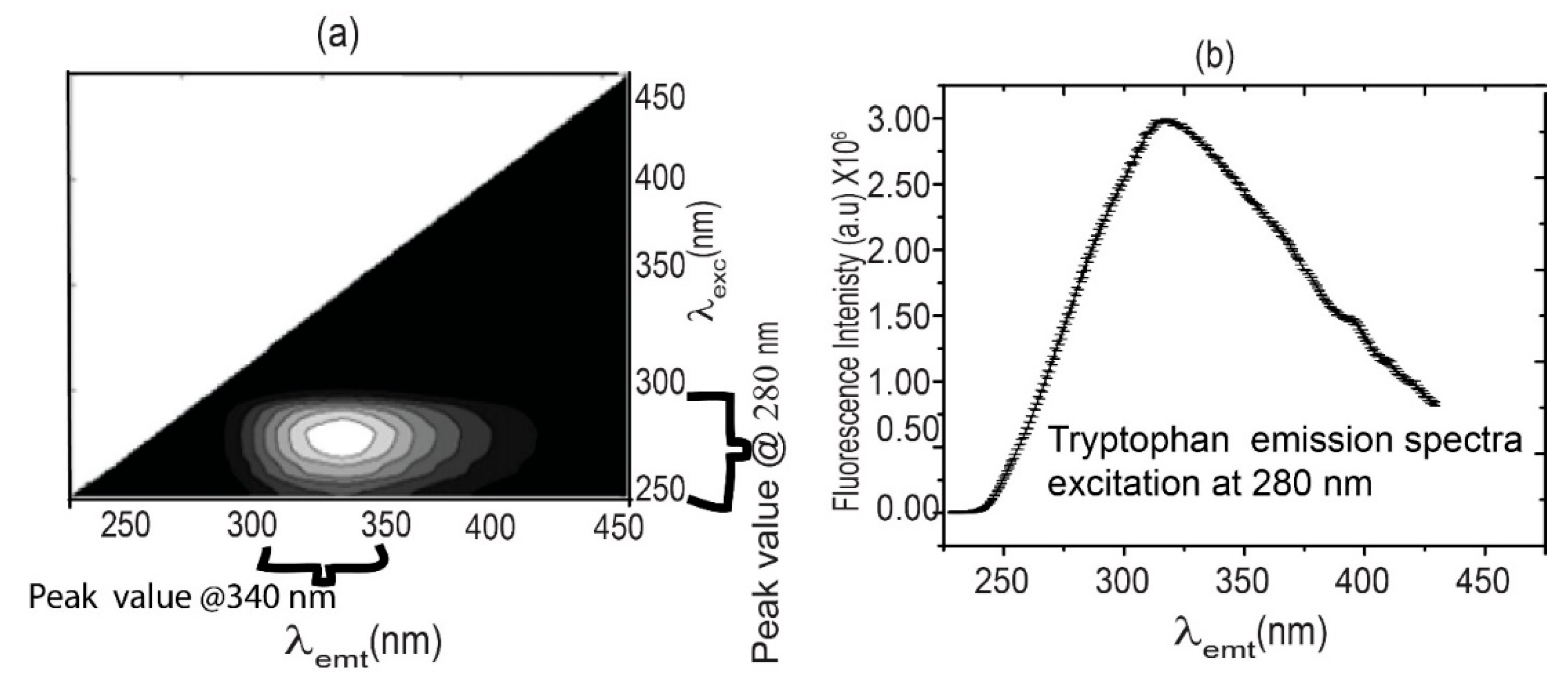
Figure 2.
Emission spectra of three florophors from blood sera, (a) Tryptophan spectra excitaion@280 nm emission range 300-500 nm, (b) NADH spectra excitaion@340 nm emission range 375-600 nm and (c) FAD spectra excitaion@365 nm emission range 440-640 nm.
Figure 2.
Emission spectra of three florophors from blood sera, (a) Tryptophan spectra excitaion@280 nm emission range 300-500 nm, (b) NADH spectra excitaion@340 nm emission range 375-600 nm and (c) FAD spectra excitaion@365 nm emission range 440-640 nm.
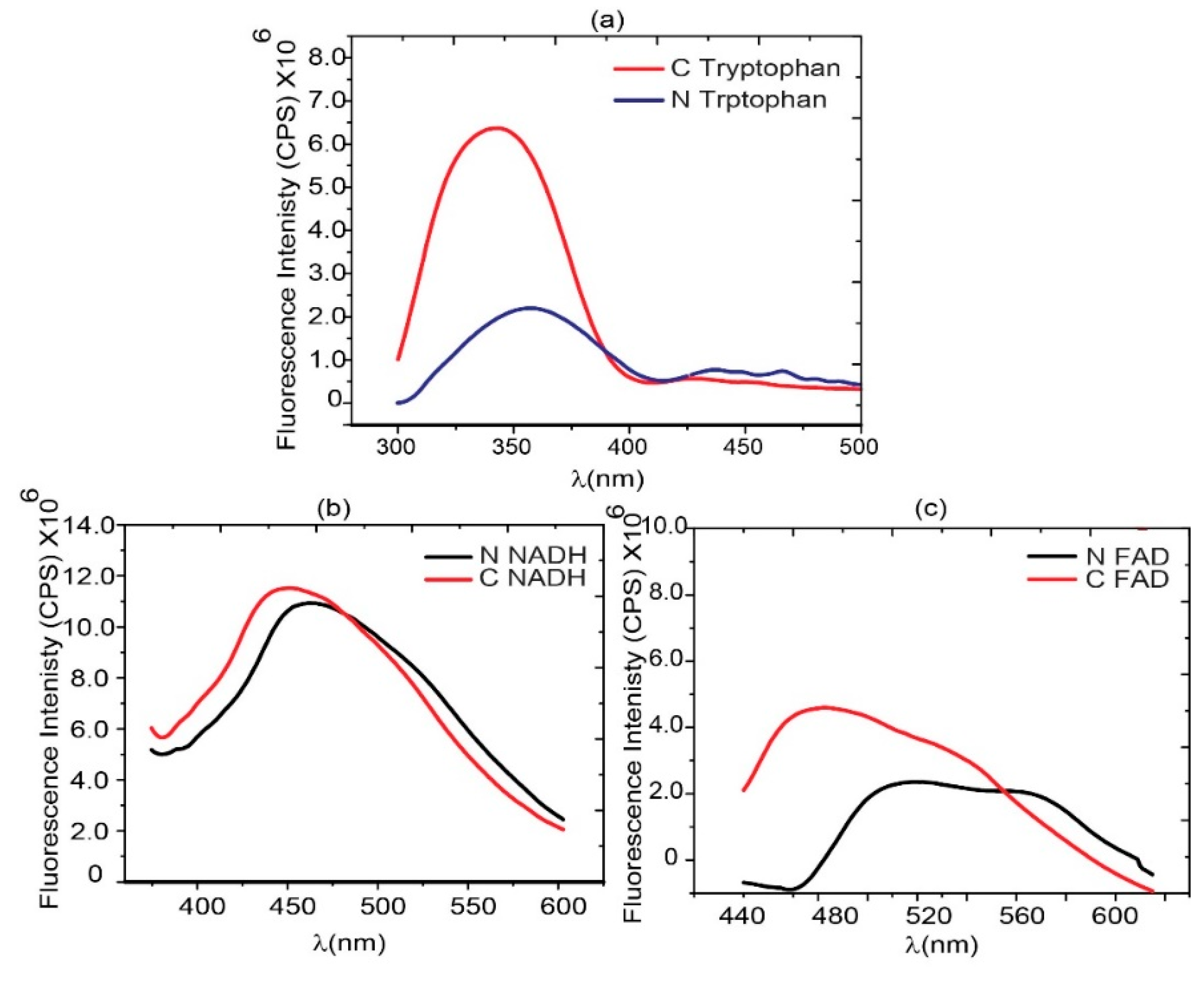
Figure 3.
The DIC image on left side of phomicrograph (a-c) at 20×, 40×, and 100× show normal cells. It shows benign breast ducks with intact myoepithelial layer. The images on right side of phomicrograph (d-f)at 20×, 40×, and 100× show malignant epithelial cells, dischohesive, the nuclei are deeply hyper chromatic, pleomorphic with inconspicuous to vesicular nuclei.
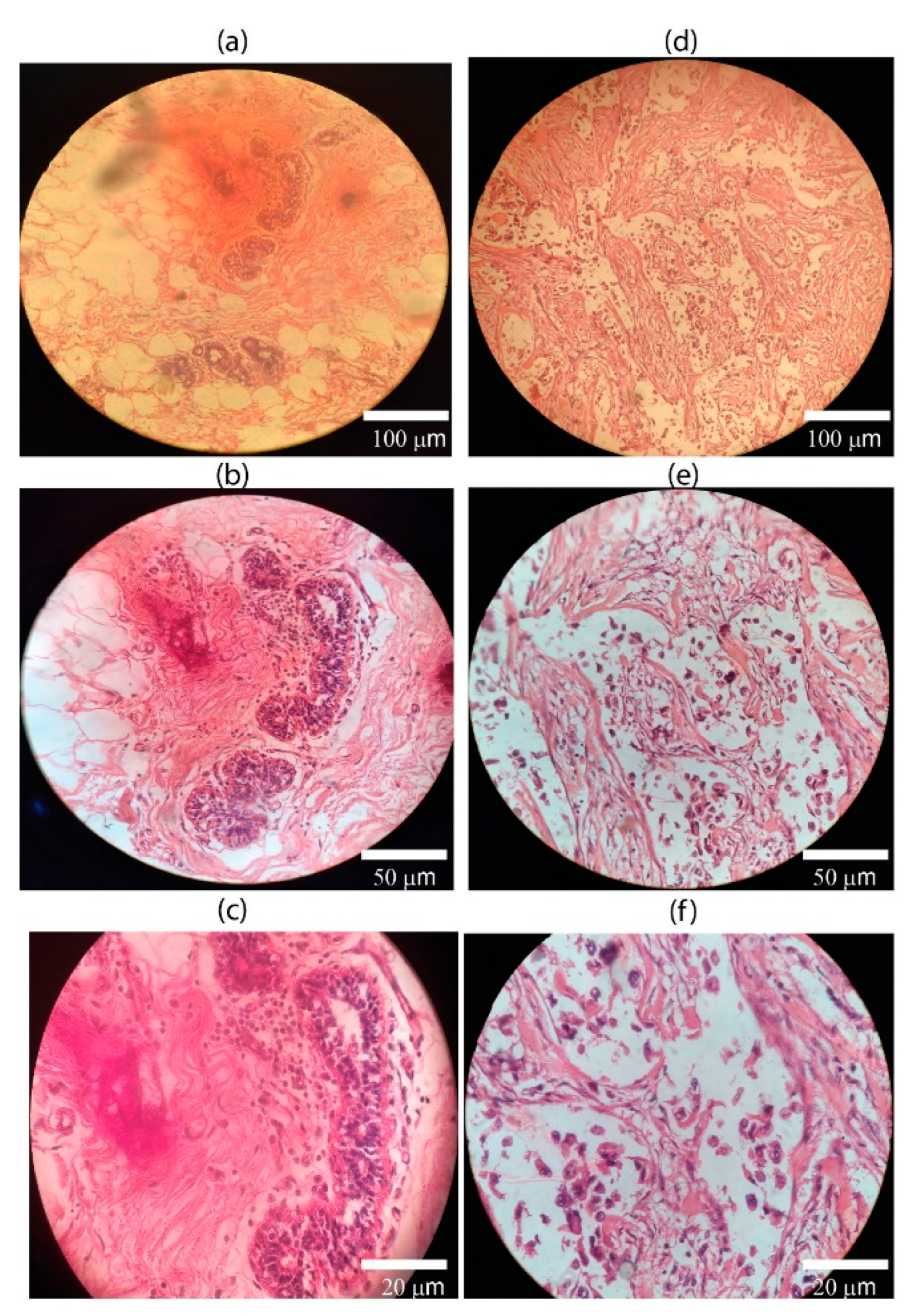
Figure 4.
Confocal auto-fluorescence microscopy of normal and cancerous breast patient’s tissue. Excitation @ λexc = 458 nm, 488 nm and 514 nm laser light with 95% transmission. Main beam splitter (HFT) 458/514 and NFT 515 with mirror depicted in green auto fluorescence, necrotic tissues (excitation λexc = 458 nm, Main beam splitter (HFT) 458/514, NFT 515 in Reddish are visible. Tissue area of (1179.13 × 1179.13) μm2 was scanned and an average of 18 images were obtained. The images on right side of phomicrograph (a-c ) at an objective Ec-Plane 20X/1.3 M27 Oil DIC, an objective Ec-Plane 40X/1.3 M27 Oil DIC and an objective Neofluar Plan-Apochromat 100x/1.40 Oil DIC M27 respectively taken for normal cells. The images on right side of phomicrograph (a-c ) at an objective Ec-Plane 20X/1.3 M27 Oil DIC, an objective Ec-Plane 40X/1.3 M27 Oil DIC and an objective Neofluar Plan-Apochromat 100x/1.40 Oil DIC M27 respectively taken for cancer cells.
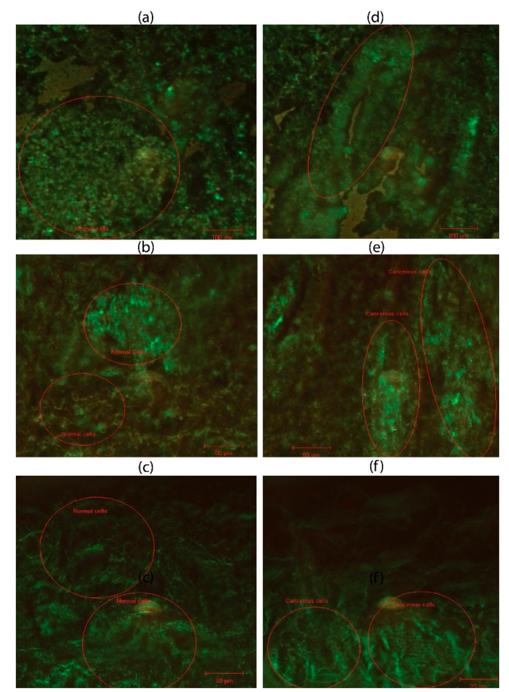
Figure 5.
GPR results for C-tryptophan: actual data (a), predicted data (b), and the corresponding error (c) between (a) and (b). A combined view of (a), (b), and (c) is presented in (d). For N-tryptophan, the GPR results are shown as actual data €, predicted data (f), and error (g) between € and (f). A merged trend of actual, predicted, and error data is displayed in (h).
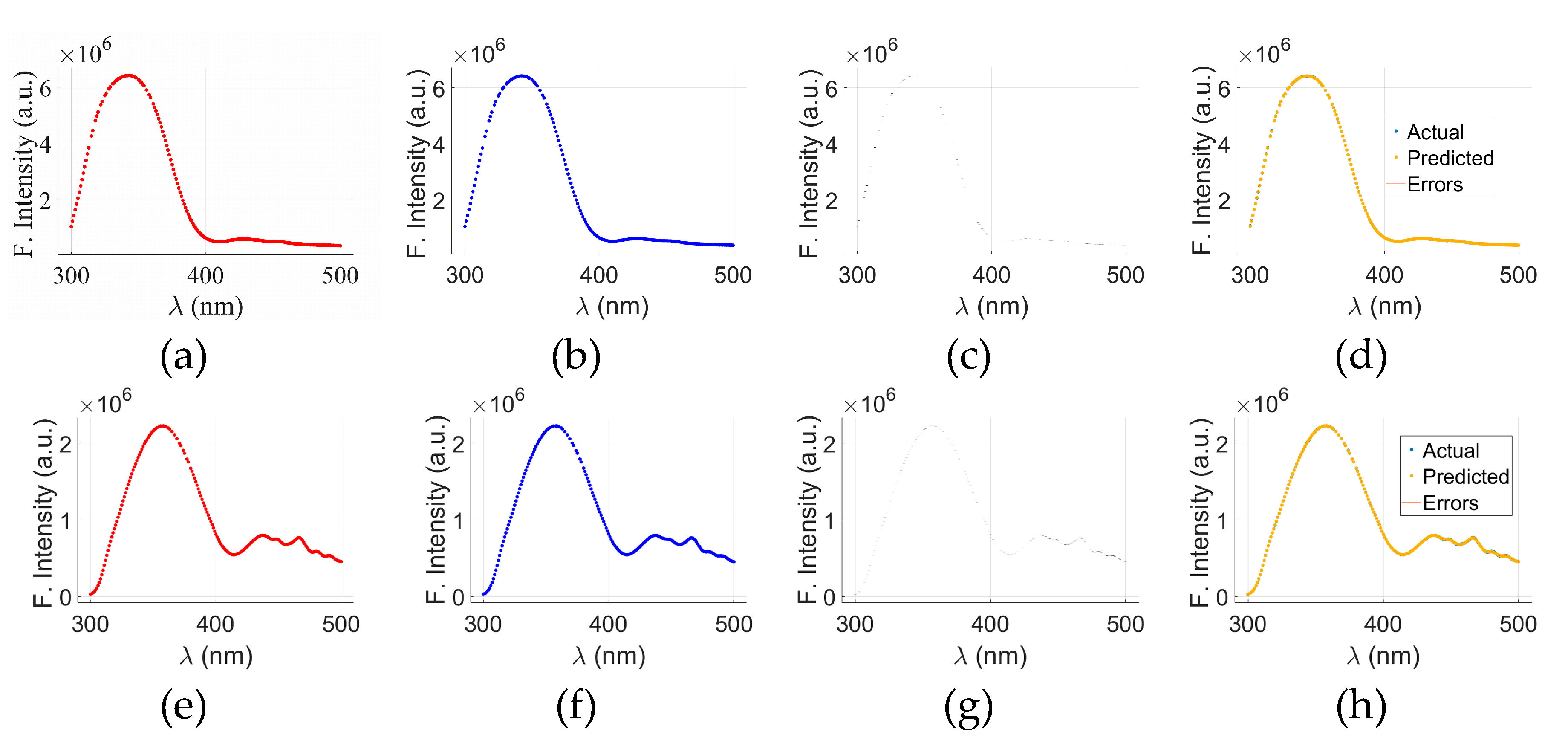
Figure 6.
C-tryptophan-based results for Models 2, 3, 4, and 5 are shown in (a), (b), (c), and (d), respectively, while N-tryptophan-based results for the same models are presented in (e), (f), (g), and (h). PvA plots using the GPR model for C-tryptophan and N-tryptophan are shown in (i) and (k), respectively. PvA plots specifically for Model 5 are illustrated in (j) for C-tryptophan and (l) for N-tryptophan.
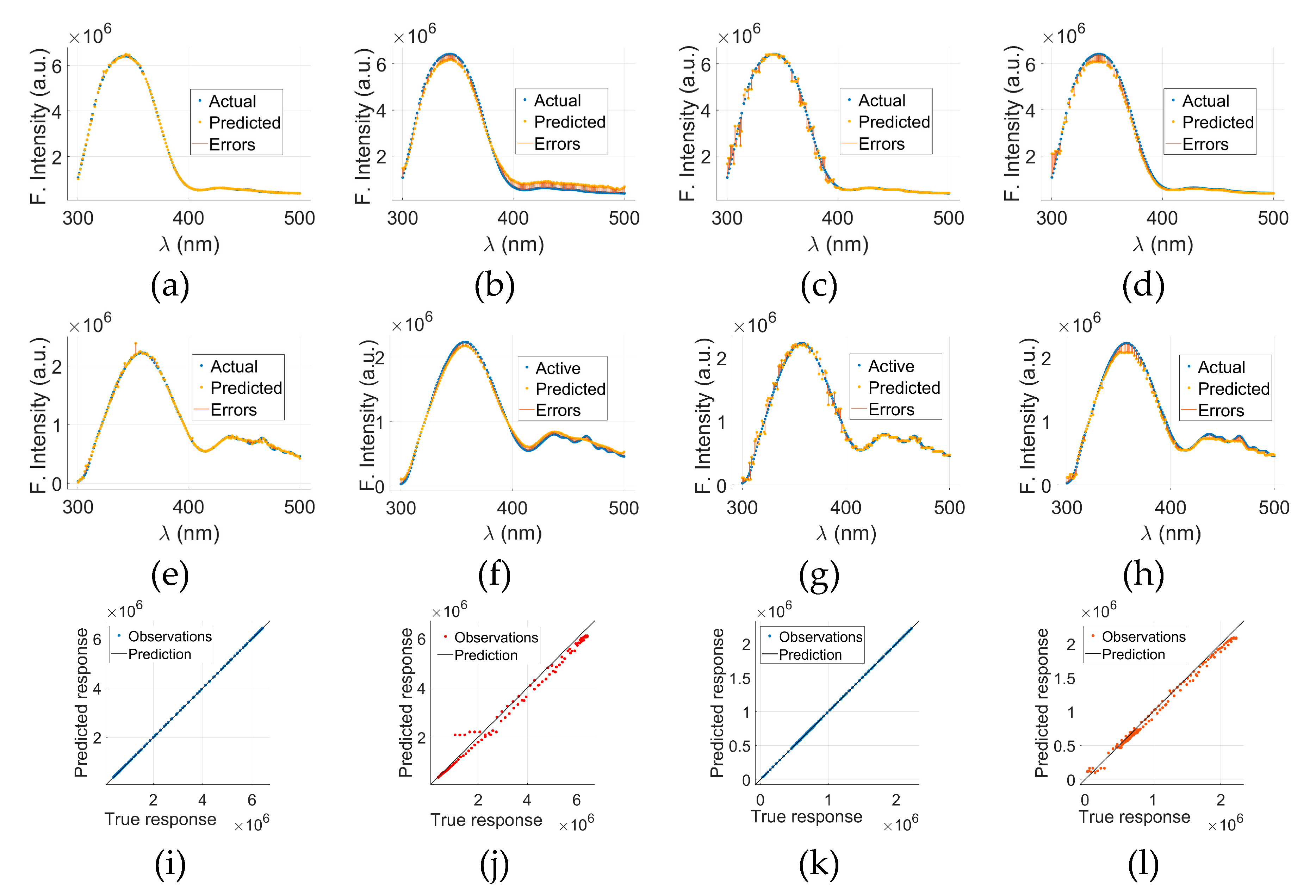
Figure 7.
GPR results for C-NADH: actual data (a), predicted data (b), and the corresponding error (c) between (a) and (b). A combined view of (a), (b), and (c) is presented in (d). For N-NADH, the GPR results are shown as actual data (e), predicted data (f), and error (g) between (e) and (f). A merged trend of actual, predicted, and error data is displayed in (h).
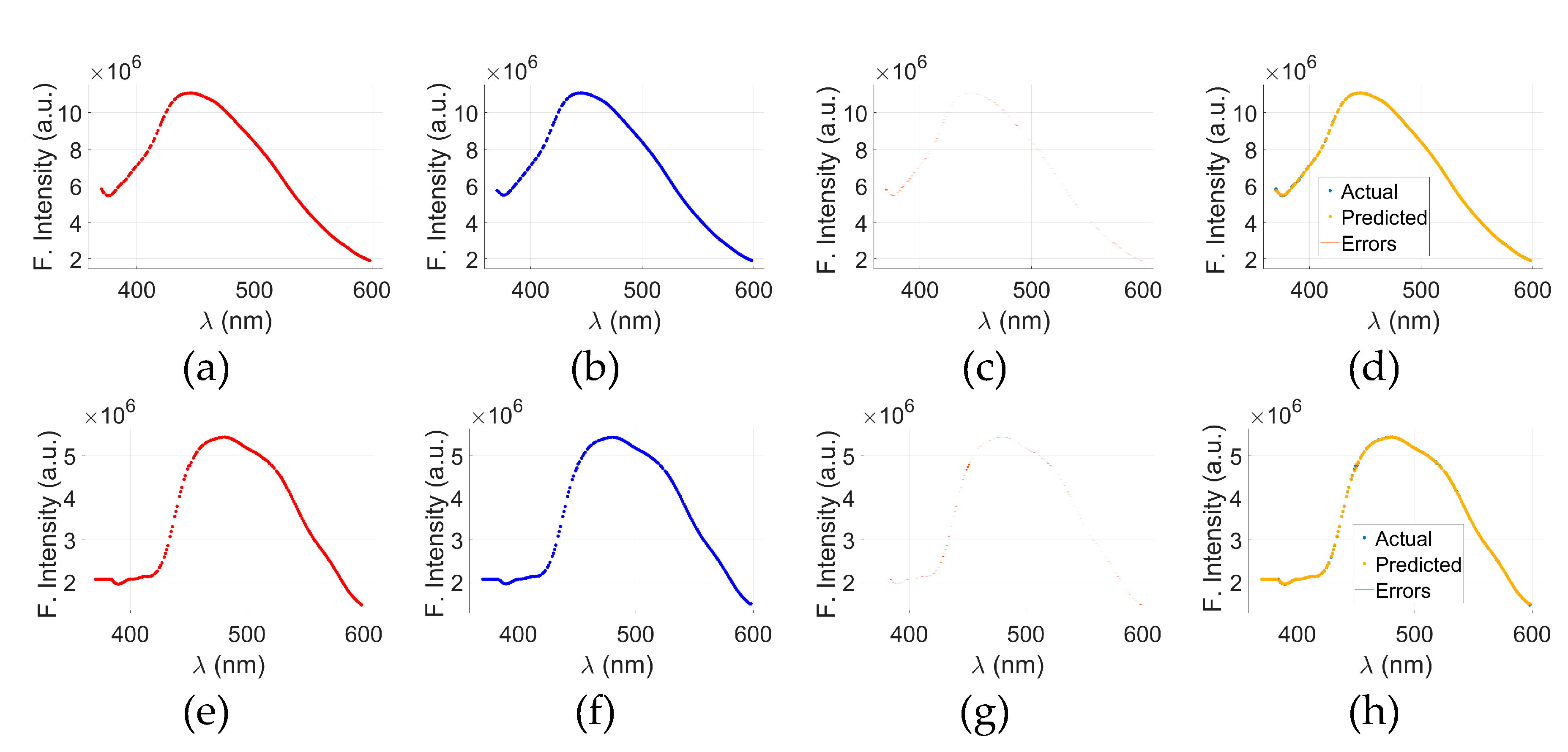
Figure 8.
C-NADH-based results for Models 2, 3, 4, and 5 are shown in (a), (b), (c), and (d), respectively, while N-NADH-based results for the same models are presented in (e), (f), (g), and (h). PvA plots using the GPR model for C-and N-NADH are shown in (i) and (k), respectively. PvA plots specifically for Model 5 are illustrated in (j) for C-NADH and (l) for N-NADH.
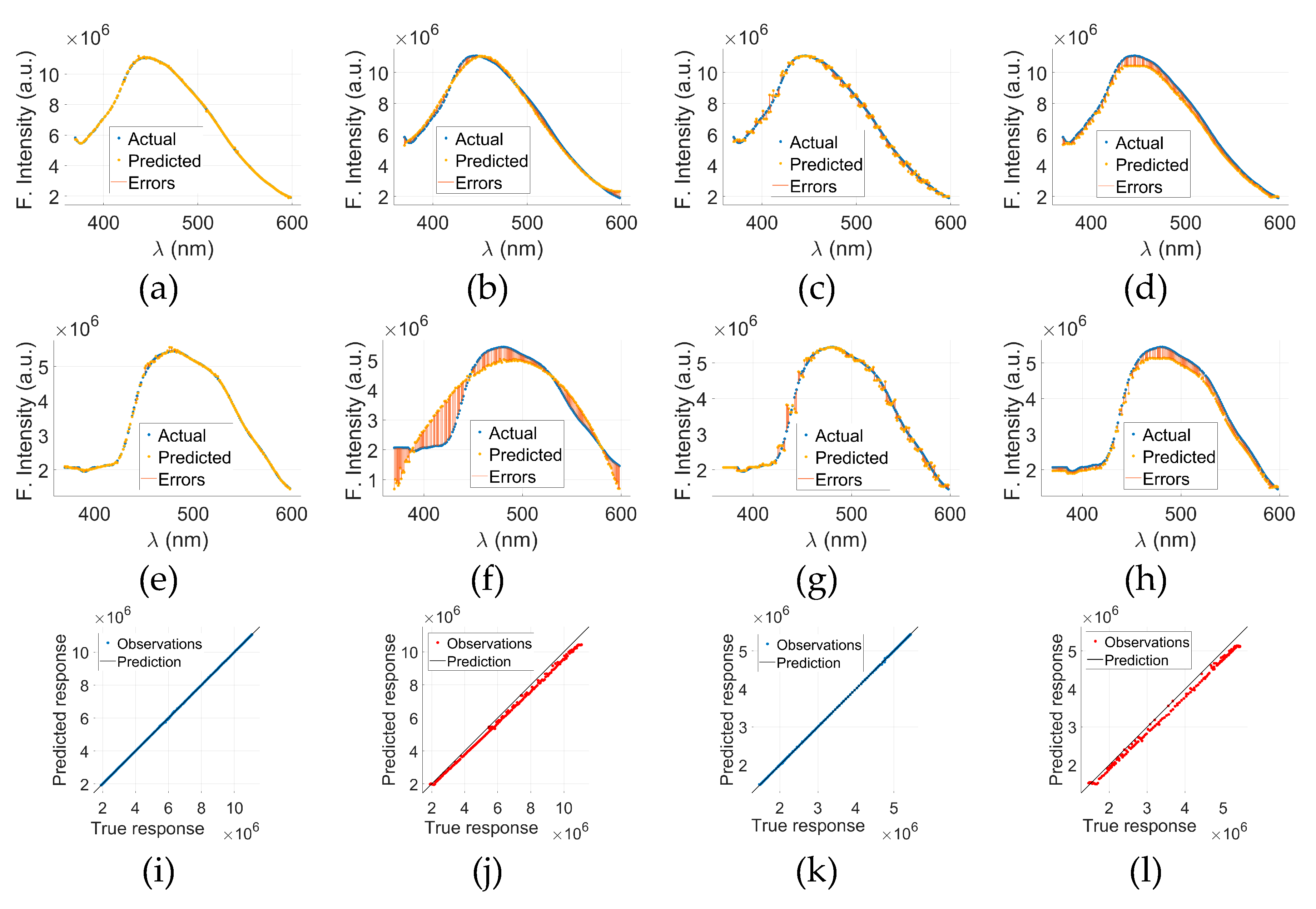
Figure 9.
GPR results for C-FAD: actual data (a), predicted data (b), and the corresponding error (c) between (a) and (b). A combined view of (a), (b), and (c) is presented in (d). For N-FAD, the GPR results are shown as actual data (e), predicted data (f), and error (g) between (e) and (f). A merged trend of actual, predicted, and error data is displayed in (h).
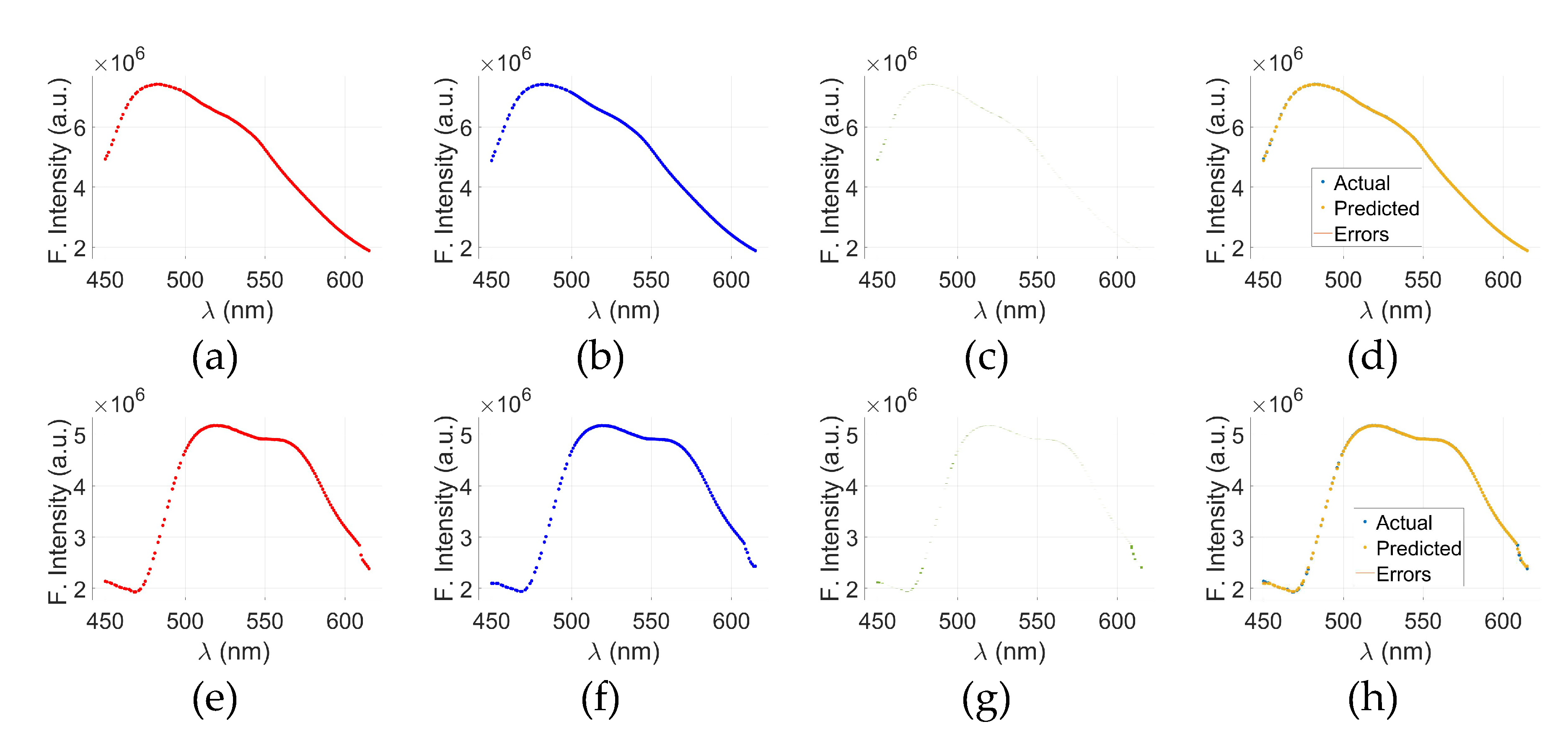
Figure 10.
C-FAD -based results for Models 2, 3, 4, and 5 are shown in (a), (b), (c), and (d), respectively, while N-FAD -based results for the same models are presented in (e), (f), (g), and (h). PvA plots using the GPR model for C- and N-FAD are shown in (i) and (k), respectively. PvA plots specifically for Model 5 are illustrated in (j) for C-FAD and (l) for N-FAD.
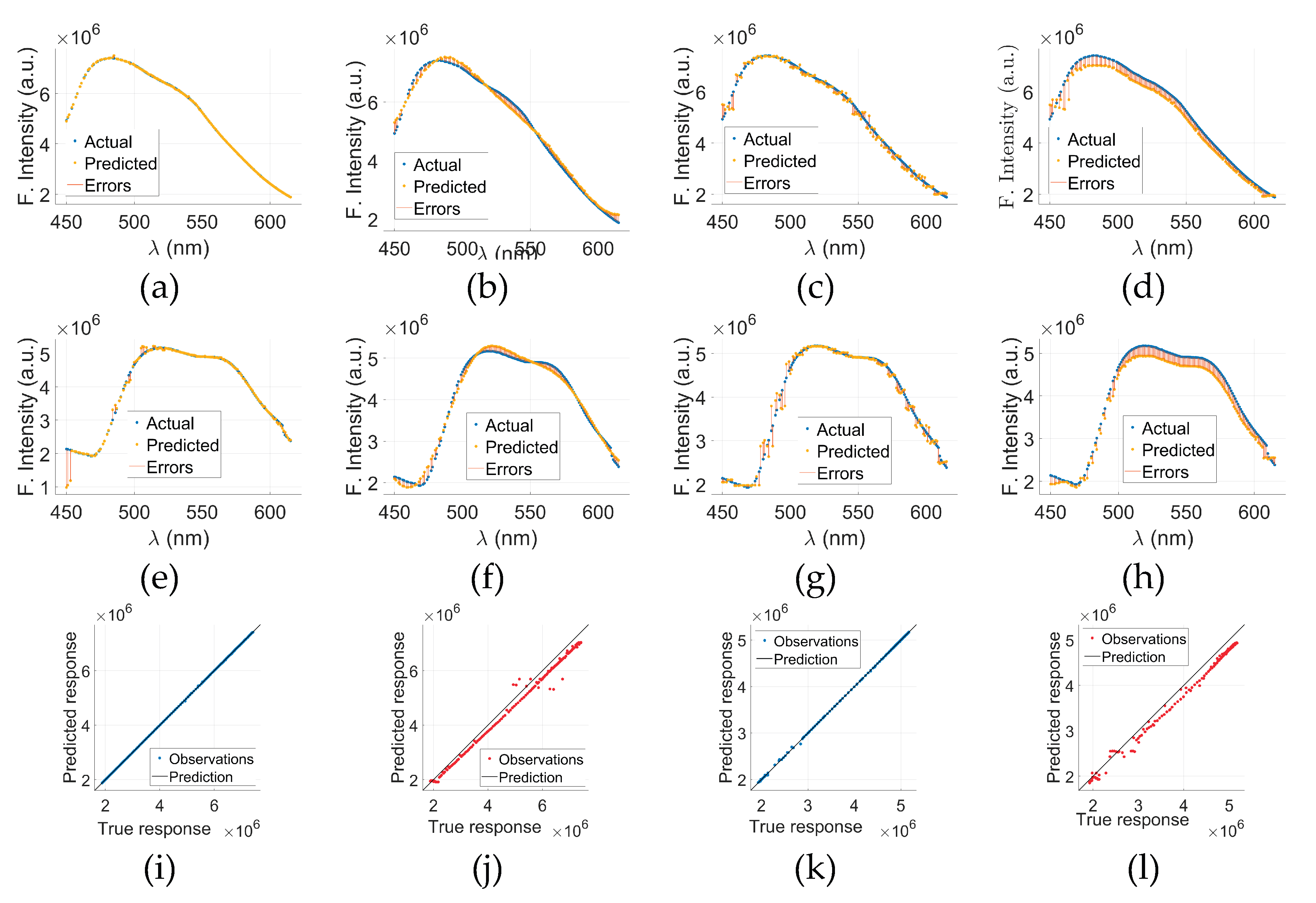

Table 1.
Fluorophores used for diagnosis with excitation/ emission peaks and their quantum yield.
| Fluorophores/ Biomarker |
Excitation Range/ Peak (nm) |
Emission Range/ Peak (nm) |
Quantum Yield |
Reference |
|---|---|---|---|---|
| Tryptophan | 280 | 350 | 0.13 | [37] |
| Tyrosine | 275 | 300 | 0.14 | [37] |
| Phenylalanine | 260 | 280 | 0.024 | [37] |
| Collagen | 325 | 400,405 | 0.1-0.4 | [38] |
| Riboflavin | 370,445 | 535 | 0.24 | [39] |
| FAD | 375,450 | 535 | 0.032 | [40] |
| NADH | 290,351 | 440,460 | 0.02-0.1 | [38] |
| NADPH | 336 | 464 | NA | [37] |
| FMN | 370,445 | 535 | 0.27 | [40] |
Table 2.
Sensitivity analysis of regression parameters validated through 10-fold cross-validation using potential regression models.
Table 2.
Sensitivity analysis of regression parameters validated through 10-fold cross-validation using potential regression models.
| Regression Model | Tuning Parameter | Seclection |
|---|---|---|
| Gaussian process regression (GPR)-Model 1 | Basis function | Constant |
| Kernel function | Matern 5/2 | |
| Use isotropic kernel | TRUE | |
| Kernel scale | Automatic | |
| Signal standard deviation | Automatic | |
| Sigma | Automatic | |
| Optimize numeric parameters | TRUE | |
| Wide Neural Networks (WNN) -Model 2 | Number of fully connected layers | 1 |
| Number of neurons | 100 | |
| Activation function | ReLU | |
| Iteration limit | 1000 | |
| Regularization strength (Lambda) | 0 | |
| Standardize data | Yes | |
| Support Vector Regression (SVR) -Model 3 | Kernel function | Gaussian |
| Kernel scale | 1 | |
| Box constraint | Automatic | |
| Epsilon | Automatic | |
| Standardize data | TRUE | |
| Fine Decision Trees (FDT) -Model 4 | Minimum leaf size | 4 |
| Surrogate decision splits | OFF | |
| Boosted Tree (BT) -Model 5 | Minimum leaf size | 8 |
| Number of learners | 30 | |
| Learning rate | 0.1 |
Table 3.
Sensitivity analysis of C-Tryptophan regression validated through 10-fold cross-validation using potential regression models. The fluorescence intensity range for C-Tryptophane is 6 × 10⁶. The direction of the arrow illustrates whether an upward or downward trend is preferred for each index.
| Regressor* | Validation (training) results** | Training (sec) |
Testing results** | ||||||
|---|---|---|---|---|---|---|---|---|---|
| RMSE↓ | R2↑ | MSE↓ | MAE↓ | RMSE↓ | R2↑ | MSE↓ | MAE↓ | ||
| GPR | 3406.5 | 1.00 | 1.2+07 | 2387.2 | 1.123 | 3621.6 | 1.00 | 1.3e+07 | 2573.2 |
| WNN | 19140.0 | 1.00 | 3.6+08 | 11297 | 6.667 | 33851.0 | 1.00 | 1.1e+09 | 28446.0 |
| SVR | 2.0e+05 | 0.99 | 4.1e+10 | 1.8e+05 | 0.478 | 2.1e+05 | 0.90 | 4.4e+10 | 1.9e+05 |
| FDT | 2.4e+05 | 0.99 | 5.7e+10 | 1.2e+05 | 0.894 | 3.4e+05 | 0.73 | 1.2e+11 | 2.6e+05 |
| BT | 2.1e+05 | 0.99 | 4.4e+10 | 1.3e+05 | 2.340 | 2.2e+05 | 0.88 | 5.0e+10 | 1.9e+05 |
*The data was standardized for GPR, WNN, and SVR. In contrast, FDT and BT, being tree-based models, are unaffected by feature scaling. After standardization, the feature values were adjusted to have zero mean and unit variance, which can reduce the interpretability of tree splits. **Performance measure percentage is calculated by dividing the value by the fluorescence intensity range (cancerious or normal) and multiplying the result by 100.
Table 4.
Sensitivity analysis of N-Tryptophan regression validated through 10-fold cross validation using fiver regression algorithms. The fluorescence intensity range for N-Tryptophane is 2 × 10⁶. The direction of the arrow illustrates whether an upward or downward trend is preferred for each index.
| Regressor* | Validation (training) results** | Training (sec) |
Testing results** | ||||||
|---|---|---|---|---|---|---|---|---|---|
| RMSE↓ | R2↑ | MSE↓ | MAE↓ | RMSE↓ | R2↑ | MSE↓ | MAE↓ | ||
| GPR | 2195.9 | 1.00 | 4.8e+06 | 1585.5 | 0.962 | 1847.5 | 1.00 | 3.4e+06 | 1391.9 |
| WNN | 15187.0 | 1.00 | 2.3e+08 | 10823.0 | 6.157 | 12750.0 | 0.99 | 1.6e+08 | 10210.0 |
| SVR | 55659.0 | 0.99 | 3.1e+09 | 46851.0 | 0.571 | 58831.0 | 0.87 | 3.5e+09 | 58426.0 |
| FDT | 72948.0 | 0.98 | 5.3e+09 | 48355.0 | 1.093 | 55683.0 | 0.89 | 3.1e+09 | 40551.0 |
| BT | 62295.0 | 0.99 | 3.9e+09 | 48893.0 | 2.319 | 1.1e+05 | 0.52 | 1.3e+10 | 1.1e+05 |
*The data was standardized for GPR, WNN, and SVR. In contrast, FDT and BT, being tree-based models, are unaffected by feature scaling. After standardization, the feature values were adjusted to have zero mean and unit variance, which can reduce the interpretability of tree splits. **Performance measure percentage is calculated by dividing the value by the fluorescence intensity range (cancerious or normal) and multiplying the result by 100.
Table 5.
Sensitivity analysis of C-NADH regression validated through 10-fold cross validation using potential regression models. The fluorescence intensity range for C-NADH is 11 × 106. The direction of the arrow illustrates whether an upward or downward trend is preferred for each index.
Table 5.
Sensitivity analysis of C-NADH regression validated through 10-fold cross validation using potential regression models. The fluorescence intensity range for C-NADH is 11 × 106. The direction of the arrow illustrates whether an upward or downward trend is preferred for each index.
| Regressor* | Validation (training) results** | Training (sec) | Testing results** | ||||||
|---|---|---|---|---|---|---|---|---|---|
| RMSE↓ | R2↑ | MSE↓ | MAE↓ | RMSE↓ | R2↑ | MSE↓ | MAE↓ | ||
| GPR | 10776.0 | 1.00 | 1.2e+08 | 6036.5 | 0.986 | 10139.0 | 1.00 | 1.0e+08 | 6791.4 |
| WNN | 36171.0 | 1.00 | 1.3e+09 | 22646.0 | 6.283 | 72781.0 | 1.00 | 5.3e+09 | 52621.0 |
| SVR | 2.1e+05 | 0.99 | 4.3e+10 | 1.7e+05 | 0.446 | 2.5e+05 | 0.98 | 6.4e+10 | 2.3e+05 |
| FDT | 2.2e+05 | 0.99 | 5.0e+10 | 1.7e+05 | 0.879 | 2.4e+05 | 0.99 | 6.0e+10 | 1.7e+05 |
| BT | 3.6e+05 | 0.98 | 1.3e+11 | 3.2e+05 | 2.241 | 3.6e+05 | 0.97 | 1.3e+11 | 3.2e+05 |
*The data was standardized for GPR, WNN, and SVR. In contrast, FDT and BT, being tree-based models, are unaffected by feature scaling. After standardization, the feature values were adjusted to have zero mean and unit variance, which can reduce the interpretability of tree splits.**Performance measure percentage is calculated by dividing the value by the fluorescence intensity range (cancerious or normal) and multiplying the result by 100.
Table 6.
Sensitivity analysis of N-NADH regression validated through 10-fold cross-validation using potential regression models.The fluorescence intensity range for N-NADH is 6 × 10⁶. The direction of the arrow illustrates whether an upward or downward trend is preferred for each index.
Table 6.
Sensitivity analysis of N-NADH regression validated through 10-fold cross-validation using potential regression models.The fluorescence intensity range for N-NADH is 6 × 10⁶. The direction of the arrow illustrates whether an upward or downward trend is preferred for each index.
| Regressor* | Validation (training) results** | Training (sec) |
Testing results** | ||||||
|---|---|---|---|---|---|---|---|---|---|
| RMSE↓ | R2↑ | MSE↓ | MAE↓ | RMSE↓ | R2↑ | MSE↓ | MAE↓ | ||
| GPR | 6866.4 | 1.00 | 4.7e+07 | 3959.8 | 1.125 | 4917.6 | 1.00 | 2.4e+07 | 3683.8 |
| WNN | 4.3e+05 | 0.90 | 1.9e+11 | 1.5e+05 | 6.865 | 5.4e+05 | 0.84 | 3.0e+11 | 4.8e+05 |
| SVR | 1.6e+05 | 0.99 | 2.7e+10 | 1.4e+05 | 0.490 | 2.0e+05 | 0.98 | 4.1e+10 | 1.8e+05 |
| FDT | 1.4e+05 | 0.99 | 2.0e+10 | 87593.0 | 1.018 | 2.0e+05 | 0.98 | 3.9e+10 | 1.1e+05 |
| BT | 1.8e+05 | 0.98 | 3.1e+10 | 1.6e+05 | 2.655 | 1.6e+05 | 0.99 | 2.5e+10 | 1.3e+05 |
*The data was standardized for GPR, WNN, and SVR. In contrast, FDT and BT, being tree-based models, are unaffected by feature scaling. After standardization, the feature values were adjusted to have zero mean and unit variance, which can reduce the interpretability of tree splits.**Performance measure percentage is calculated by dividing the value by the fluorescence intensity range (cancerious or normal) and multiplying the result by 100.
Table 7.
Sensitivity analysis of C-FAD regression validated through 10-fold cross-validation using potential regression models. The fluorescence intensity range for C-FAD is 7.5 × 10⁶. The direction of the arrow illustrates whether an upward or downward trend is preferred for each index.
Table 7.
Sensitivity analysis of C-FAD regression validated through 10-fold cross-validation using potential regression models. The fluorescence intensity range for C-FAD is 7.5 × 10⁶. The direction of the arrow illustrates whether an upward or downward trend is preferred for each index.
| Regressor* | Validation (training) results** | Training (sec) |
Testing results** | ||||||
|---|---|---|---|---|---|---|---|---|---|
| RMSE↓ | R2↑ | MSE↓ | MAE↓ | RMSE↓ | R2↑ | MSE↓ | MAE↓ | ||
| GPR | 6776.0 | 1.00 | 4.3e+08 | 6237.6 | 0.862 | 5858.5 | 1.00 | 3.4e+07 | 4065.9 |
| WNN | 19715.0 | 1.00 | 3.9e+08 | 10956.0 | 5.601 | 9404.9 | 1.00 | 8.8e+07 | 7479.8 |
| SVR | 1.6e+05 | 0.99 | 2.5e+10 | 1.3e+05 | 0.413 | 1.6e+05 | 0.94 | 2.6e+10 | 1.4e+05 |
| FDT | 2.0e+05 | 0.99 | 4.0e+10 | 1.3e+05 | 1.222 | 1.4e+05 | 0.95 | 1.9e+10 | 81553.0 |
| BT | 3.2e+05 | 0.97 | 1.0e+11 | 2.8e+05 | 2.400 | 3.6e+05 | 0.68 | 1.3e+11 | 3.2e+05 |
*The data was standardized for GPR, WNN, and SVR. In contrast, FDT and BT, being tree-based models, are unaffected by feature scaling. After standardization, the feature values were adjusted to have zero mean and unit variance, which can reduce the interpretability of tree splits.**Performance measure percentage is calculated by dividing the value by the fluorescence intensity range (cancerious or normal) and multiplying the result by 100.
Table 8.
Sensitivity analysis of N-FAD regression validated through 10-fold cross-validation using potential regression models. The fluorescence intensity range for N-FAD is 5 × 10⁶. The direction of the arrow illustrates whether an upward or downward trend is preferred for each index.
Table 8.
Sensitivity analysis of N-FAD regression validated through 10-fold cross-validation using potential regression models. The fluorescence intensity range for N-FAD is 5 × 10⁶. The direction of the arrow illustrates whether an upward or downward trend is preferred for each index.
| Regressor* | Validation (training) results** | Training (sec) |
Testing results** | ||||||
|---|---|---|---|---|---|---|---|---|---|
| RMSE↓ | R2↑ | MSE↓ | MAE↓ | RMSE↓ | R2↑ | MSE↓ | MAE↓ | ||
| GPR | 3207.0 | 1.00 | 1.2e+08 | 3188.4 | 1.008 | 2819.5 | 1.00 | 7.9e+06 | 2444.6 |
| WNN | 29584.0 | 1.00 | 8.7e+08 | 19776.0 | 7.663 | 12109.0 | 1.00 | 1.5e+08 | 9177.1 |
| SVR | 1.1e+05 | 0.99 | 1.3e+10 | 96538.0 | 0.509 | 1.4e+05 | 0.97 | 2.1e+10 | 1.3e+05 |
| FDT | 1.5e+05 | 0.98 | 2.2e+10 | 89525.0 | 0.986 | 1.9e+05 | 0.95 | 3.8e+10 | 1.3e+05 |
| BT | 2.0e+05 | 0.97 | 4.0e+10 | 1.9e+05 | 2.272 | 81137.0 | 0.99 | 6.6e+09 | 67678.0 |
*The data was standardized for GPR, WNN, and SVR. In contrast, FDT and BT, being tree-based models, are unaffected by feature scaling. After standardization, the feature values were adjusted to have zero mean and unit variance, which can reduce the interpretability of tree splits.**Performance measure percentage is calculated by dividing the value by the fluorescence intensity range and multiplying the result by 100.
Disclaimer/Publisher’s Note: The statements, opinions and data contained in all publications are solely those of the individual author(s) and contributor(s) and not of MDPI and/or the editor(s). MDPI and/or the editor(s) disclaim responsibility for any injury to people or property resulting from any ideas, methods, instructions or products referred to in the content. |
© 2025 by the authors. Licensee MDPI, Basel, Switzerland. This article is an open access article distributed under the terms and conditions of the Creative Commons Attribution (CC BY) license (http://creativecommons.org/licenses/by/4.0/).
Copyright: This open access article is published under a Creative Commons CC BY 4.0 license, which permit the free download, distribution, and reuse, provided that the author and preprint are cited in any reuse.


