Climate, Water Vapor, and Volcanic Eruptions

J. Higginbotham

doi:10.20944/preprints202508.2148.v1

Submitted:

23 August 2025

Posted:

29 August 2025

You are already at the latest version

Abstract

The objective is to stimulate research into alternative mechanisms that might increase sustained water vapor in the atmosphere and thus drive climate warming. Toward this end a period from the prior interglacial from 130,000 BCE to 110,000 BCE is examined to show that temperature peaks and atmospheric concentration of CO2 reaches its maximum level, then temperature falls by 7 to 8 degrees C over 13,000 years while atmospheric CO2 concentration remains high and constant. Mechanisms that might support this cooling while CO2 remains high and constant are considered. It is noted that the primary assumed source of climate warming is a sustained higher level of water vapor. Current measurements of water vapor are examined. An apparent connection with volcanic eruptions having Volcanic Explosivity Index (VEI) of 5 or greater is noted in the water vapor data for the upper atmosphere. This is suggested as a mechanism that contaminates our atmospheric water vapor measurements to induce a high level of noise from a source disconnected from climate. This noise interferes with efforts to determine or verify the source of sustained atmospheric water vapor. Mechanisms that might cause climate warming while bypassing a CO2 forcing are suggested that involve variations in cloud cover.

Keywords:

Watervapor

;

volcanos

;

clouds

Subject:

Environmental and Earth Sciences - Atmospheric Science and Meteorology

Introduction

The discussion will begin by considering (1) Milankovitch orbital cycles, (2) a time interval of Antarctic ice core data for both temperature and CO2, (3) CO2 and water vapor calculations leading to climate temperature rise, and finally (4) water vapor measurements and volcanic eruptions.

The objective is to raise for consideration the possibility that a sustained concentration of water vapor in our atmosphere is controlled by mechanisms other than the CO2 green house gas. The further objective is to stimulate research into other possible mechanisms for sustained increased atmospheric water vapor.

A quote from Physical Geology [1]:

… climate feedbacks are critically important in amplifying weak climate forcings into full-blown climate changes. When Milankovitch published his theory in 1924, it was widely ignored, partly because it was evident to climate scientists that the forcing produced by the orbital variations was not strong enough to drive the significant climate changes of the glacial cycles. Those scientists did not recognize the power of positive feedbacks. It wasn’t until 1973, 15 years after Milankovitch’s death, that sufficiently high-resolution data were available to show that the Pleistocene glaciations were indeed driven by the orbital cycles, and it became evident that the orbital cycles were just the forcing that initiated a range of feedback mechanisms that made the climate change.

This viewpoint, as well as why water vapor gets downplayed, is also well represented by the MIT Climate Portal:

https://climate.mit.edu/ask-mit/why-do-we-blame-climate-change-carbon-dioxide-when-water-vapor-much-more-common-greenhouse

If we look at Antarctic Ice Core data over the last 800,000 years in particular, we find this warming process reversed and the climate falls into deep cooling of the atmosphere – top of Figure 1, showing this for the prior interglacial warm period. A plot of this same data over 800,000 years, with apparent smoothing, is found at https://www.bas.ac.uk/data/our-data/publication/ice-cores-and-climate-change/ Figure 3, but the reader must zoom in on the specific time interval to compare (this external figure caption references Parrenin, F. et al., https://doi.org/10.1126/science.1226368 ).

It should be clear that to drive climate into a glacial when all these feedback mechanisms have been enabled, it is then required to either find a way to turn them all off when they have reached their maximum effect or find a forcing that can overcome these powerful feedback mechanisms when at their maximum.

Data from the prior interglacial shown in Figure 1 will be considered along with more modern data for water vapor. These will be somewhat difficult to tie together since water vapor data is not available for the period shown in Figure 1. However both sets of data are important to the objective of this article.

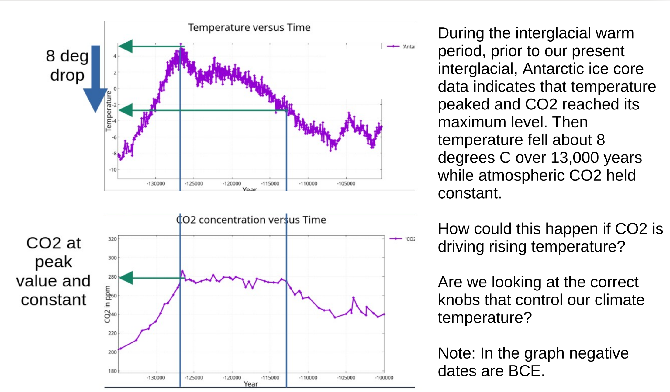
Here, in Figure 1, we see that CO2 maintains its highest level for that interglacial for 13,000 years while temperature falls 7 to 8 degrees C. If the “power of positive feedback” is required to cause temperature to rise because the orbital influence is too weak and the feedback mechanisms have reached their maximum levels producing peak temperature, then how can temperature fall 8 degrees C under these conditions? A 13,000 year period is unlikely to be explained by transient events.

External Forcings

Logical Issues

Given the statement:

All cases of high atmospheric CO2 concentration are associated with rising climate temperature.

This statement is found to be logically false based on the data shown in Figure 1.

So let’s modify the statement to be correct.

All cases of high atmospheric CO2 concentration are associated with rising climate temperature except in special cases where transient events may cause temperature to fall when atmospheric CO2 concentration is high.

So now we have to evaluate the data in Figure 1 above to decide if perhaps some transient event was involved. Exactly what does “transient” mean when CO2 concentration remained constant for 13,000 years while temperature was falling? Even on the scale of a climate change event, 13,000 years is a long time. The Younger Dryas was a major climate event but it happened over a time interval of less than 2000 years. The entire Holocene (our current interglacial) is only 11,700 years old.

Ice Sheet Growth and Ocean Current

The period from 130,000 BCE to 110,000 BCE corresponds to the height of an interglacial period that peaked at about 127,000 BCE with that interglacial warm period sustained until at least 117,000 BCE. Therefore even though temperature was falling during this time interval it is unlikely that ice sheets were growing sufficiently to induce this cooling, especially initiation of this cooling, (https://www.esd.ornl.gov/projects/qen/nercEUROPE.html ).

Plankton indicators of north Atlantic surface temperatures and deep Atlantic circulation patterns appear to corroborate this event, suggesting that the north Atlantic climate experienced a sudden cool phase resulting from a weakening of the Gulf Stream (lasting perhaps several centuries) at about 121,000 or 122,000 y.a. (Maslin 1996). After this the climate never returned to its previous warmth, although the pollen records seem to suggest that conditions more similar to those of today, lasting for perhaps 5,000 years up until around 115,000 y.a.

The reference to Maslin [4] indicates:

Based on the absence of IRD and other evidence of melting icebergs [5,7] during the peak Eemian, the observed freshening of the surface waters and the corresponding reduction of deep-water formation cannot be ascribed to a mystical ice surge event, ….

And:

We therefore conclude that the E e m i a n / M I S 5e was, at least in the subtropics, and we infer globally, climatically relatively stable, the exception being a brief cold event lasting no longer than 400 years, which may have had a profound short-term effect, but no long-term influence on the climate of the Northern Hemisphere.

“The Gulf Stream is part of a larger circulation system called the Atlantic Meridional Overturning Circulation (AMOC)” as stated at https://skepticalscience.com/print.php?n=975 . This ocean current has a role in maintaining a mild climate in Northern Europe. If this current were interrupted then the North Atlantic could become colder and induce increased snow and ice in the north, on Greenland in particular.

Hodell et al. [5] indicate:

We suggest that low- δ¹³C water and slow current speed on Gardar Drift during the early part of the [Last Interglacial] LIG was related to increased melt water fluxes to the Nordic Seas during peak boreal summer insolation, which decreased the flux and/or density of overflow to the North Atlantic. The resumption of the typical interglacial pattern of strong, well-ventilated Iceland Scotland Overflow Water was delayed until ∼ 124 ka. These changes may have affected Atlantic Meridional Overturning Circulation.

And:

Although future greenhouse gas forcing will be different than the insolation forcing of the LIG, our findings indicate that circulation on the Gardar Drift was weaker during the earliest part of the LIG when climate was warmer than present and the Greenland ice sheet was retreating ….

Since typical interglacial patterns resumed at approximately ~124 ka (~122 BCE), this seems an unlikely mechanism for extended cooling through 110,000 BCE though it might account for earlier cooling. Yet during the earliest part of the last interglacial Greenland’s ice sheet was retreating.

Ice sheet growth and/or a modification of ocean currents are complex processes and identifying evidence of these and associating a cause for a time removed from the present by over 112,000 years is a challenge. What can be said is that if these initiated the cooling shown in Figure 1 then those mechanisms did so while CO2 was at its highest atmospheric concentration of the prior interglacial period and constant for 13,000 years presumably with all feedback mechanisms active.

Clouds

We have the statement [6}:

At any given time, about two-thirds of Earth's surface is covered by clouds. Overall, they make the planet much cooler than it would be without them.

Clouds help to keep Earth cool by reflecting sunlight back out to space before it can reach the ground. But not all clouds are equal.

Shiny, white clouds reflect away more sunlight—especially when they are closer to the equator, in the parts of Earth that receive the most sun. Gray, broken clouds reflect less sunlight, as do clouds closer to the poles where less light falls.

Research published last year showed that Earth has been absorbing more sunlight than the greenhouse effect alone can explain. Clouds were involved, but it wasn't clear exactly how.

It would be disingenuous to ignore the Nobel prize laureate John Clauser’s statements here. He is quoted as saying:

When clouds are added to climate models, it’s clear that there is no ‘climate emergency,’ Dr. John Clauser argues.

See: https://climaterealists.ca/clouds-not-co2-key-to-understanding-climate-nobel-winner/

We have no way of knowing or describing cloud cover between 130,000 BCE and 110,000 BCE. Therefore cloud cover variation, of the proper type, may have been the cause of cooling seen in Figure 1. The assumed associated rise in water vapor and CO2 were then overcome by rising cloud cover. Given “rising water vapor” it seems reasonable to expect rising cloud cover at some point, though if water vapor is currently rising the above reference seems to be in conflict, at least in the short term.

Volcanic Eruptions

A single volcanic eruption might block solar radiation for a few years at most. Only a sequence of volcanic eruptions, with short intervals between, over this 13,000 year period might explain the observed fall in temperature.

The Old Crow eruption ejected ~200 cubic km of ash and was dated at ~125,000 yr but more recent dating, Burgess et al. [7] has indicated an eruption date of 207 +- 13 kyr . As a result the Old Crow tephra is not evidence for unusual volcanic activity or direct climate impact within the 130,000-110,000 BCE interval. Interpretations relying on the previous ~125,000 year age must be revised.

There is currently no evidence of sustained volcanic activity over the subject 13,000 year period.

Meteor or Comet Impacts

What about meteor or comet impacts? No confirmed large meteor or comet strikes are known to have occurred between 130,000 and 110,000 BCE. Consulting the Earth Impact Database (Planetary and Space Science Centre (PASSC) University of New Brunswick Fredericton, New Brunswick, Canada) athttp://www.passc.net/EarthImpactDatabase/New%20website_05-2018/Agesort.htmlthere are two impacts to consider. (1) Hickman in Australia with diameter 0.26 km and, (2) Amguid in Algeria with diameter 0.45 km. For comparison, Barringer crater (also known as Meteor Crater) in Arizona, USA has a diameter of 1.18 km and is 49,000 years old. Hickman and Amguid appear to be too small to have had a lasting influence. The world map of identified craters indicates very few have been identified in the oceans suggesting that many impacts are unknown.

A quote from the PASSC web site:

Model calculations indicate that it does not require a K-T-sized event, which produced the buried 180 km diameter Chicxulub impact structure in the Yucatan, Mexico, to result in atmospheric blow-out. Relatively small impact events, resulting in impact structures in the 20 km size-range can produce atmospheric blow-out. At present, however, the K-T is the only biostratigraphic boundary with a clear signal of the involvement of a large-scale impact event. The involvement of impact in other boundary events in the terrestrial stratigraphic record has been suggested but little evidence has been offered.

Impacts may also induce chemical changes in the atmosphere. These are related to the vaporization of the impacting body and a portion of the target. Considering only the contribution from the impacting body, recent calculations indicate that even relatively small impacting bodies, < 0.5 km in diameter that produce impact craters on the scale of 10 km in diameter, would inject 5 times more sulphur into the stratosphere than its present content. Larger impact events occurring on the time-scale of a million years will inject enough sulphur to produce a drop in temperature of several degrees and a major climatic shift.

All major boundary events that might be similar to the K-T boundary are much older than the event associated with the K-T boundary.

Unless new evidence is uncovered it is unlikely that impacts affected the climate during the subject time interval.

Solar Activity

Grand solar minima can cause increases in cosmogenic isotope production leaving radiocarbon evidence of the event. Dee et al. [8] examined the period 433-315 BCE and identified a grand solar minima around 400 BCE. Is there any similar evidence for the period from 130,000 BCE to 110,000 BCE?

The University of Chicago has a web page (https://news.uchicago.edu/explainer/what-is-carbon-14-dating ) explaining radiocarbon dating. When discussing the limitations of the method the statement made is:

Radiocarbon dating works on organic materials up to about 60,000 years of age.

Unfortunately the time interval of interest here is about twice this 60,000 year period.

So changes in solar radiation received by the Earth cannot be determined for the subject period from cosmogenic isotope production using radiocarbon dating. Changes in solar activity remain a possible explanation for the fall in temperature. We have no data available for verification.

Water Vapor and CO2

The feedback mechanisms associated with climate warming require a connection between CO2 and water vapor. Physicists have performed detailed computations using hundreds of thousands of absorption lines from a data base, taking into account absorption line broadening, and using a temperature model of the atmosphere to 80 km, van Wijngaarden et al. [9]. The resulting computation was compared with satellite data measurements in the upper atmosphere to verify their results (see Wijngaarden et al. Figure 15). The computational method has also been further applied to broaden the understanding of the greenhouse effect the earth is experiencing now [10,11].

The involvement of water vapor with CO2 is discussed by van Wijngaarden et al. [9] in Section 7.5 entitled Climate Sensitivity. This doesn't explain how, over millions of years and the last 800,000 years of ice core data in particular, you find this process reversed falling into deep cooling of the atmosphere. It should be clear that if you've enabled all these feedback mechanisms ... you then have to find a way to turn them all off, when they have reached their maximum effect, to dive climate into a glacial. This applies for every transition from interglacial warm period to glacial cold period. However, for the case shown in Figure 1 the issue is emphasized since the CO2 level remained at it’s max and near constant for 13,000 years while temperature was falling.

Wijngaarden et al [9] notes that the warming caused by doubling atmospheric CO2 from 400 ppm to 800 ppm shown in their Figure 4 to result in a forcing increase of 3.0 W/square meter in the lower atmosphere while the Earth's atmosphere receives 340 W/m2 from the Sun. The Stefan-Boltzmann law suggests that

δ T = T \frac{δ F}{4 F}

or

δ T = 293 K \frac{3 W / s q m}{4 * 340 W / s q m} = 0.65 K .

which is not a large temperature change.

The hypothesis that this small increase in temperature will induce a sustained increase in atmospheric water vapor allows the clear sky computation to predict temperature increases as high as 2.2 K for the case of Fixed relative humidity – see van Wijngaarden et al. [9], Table 5. Warmer air can hold more water so that fixed relative humidity means more water vapor – a green house gas.

Thus the feedback mechanism that is assumed to have caused the rise in temperature to a peak value in Figure 1, involved a sustained atmospheric water vapor increase but presumably no increase in cloud cover. If this is correct then the sustained peak level of atmospheric CO2 should sustain atmospheric water vapor and hold temperature high. That didn’t happen for 13,000 years starting in 127,000 BCE.

It is possible that water vapor condensed out of the atmosphere as temperature fell but taking that path of reasoning seems to implicitly declare the innocence of CO2 as a driver of rising sustained water vapor in the atmosphere.

As greenhouse gases like carbon dioxide and methane increase, Earth's temperature rises in response. This increases evaporation from both water and land areas. Because warmer air holds more moisture, its concentration of water vapor increases Steamy Relationships: How Atmospheric Water Vapor Amplifies Earth's Greenhouse
If the temperature rises, the amount of water vapor rises with it. But since water vapor is itself a greenhouse gas, rising water vapor causes yet higher temperatures. We refer to this process as a positive feedback, and it is thought to be the most important positive feedback in the climate system Why do we blame climate change on carbon dioxide, when water vapor is a much more common greenhouse gas? | MIT Climate Portal

So Milankovitch orbital cycle effects cause a slight warming releasing CO2 that then causes more warming that releases water vapor and then water vapor really starts warming the climate to generate a lot more water vapor.

The problem is that this could be better stated as: Milankovitch orbital cycle effects cause a slight warming releasing CO2 and water vapor, then CO2 generates a little warming and water vapor generates a lot more warming and a lot more water vapor. It’s not reasonable to assume that warming from orbital forcings must first cause a rise in CO2 before also causing a rise in sustained atmospheric water vapor. Higher atmospheric CO2 is not a prerequisite for higher sustained water vapor. Warming to any degree should increase both of these and water vapor is the stronger green house gas. .

Theory, observations, and modeling results all show that as global temperatures warm, the mean atmospheric moisture content increases …. Coupled with a slower rate of increase of precipitation (~1%–3% K−1 for precipitation as compared with the Clausius–Clapeyron rate of 7% K−1 for lower tropospheric water vapor; ... this leads to the conclusion that the convective mass flux of moisture from the boundary layer to the free troposphere must decrease … while the atmospheric moisture residence time must increase [12].

Water vapor begets warming begets more water vapor.

There remains the problem we see in the interglacial prior to the current where CO2 and presumably sustained water vapor reach their highest level and hold that level for 13,000 years while temperature falls significantly.

Volcanic Eruptions and Water Vapor

Measurements of water vapor at six different altitude intervals over Boulder Colorado are shown in Figure 2. These measurements were made by NOAA’s Global Monitoring Laboratory using the NOAA Frost Point Hygrometer (FPH). A quote from the web page:

Most relevant to our study is water vapor’s effects on the Earth’s energy budget, influencing both the incoming solar radiation and outgoing heat (IR). Variations in the amounts of water vapor in the atmosphere are natural and normal, but changes in its vertical distribution, especially in the upper troposphere and lower stratosphere, may be indicative of changes in the Earth’s climate.

In Figure 3 volcanic eruptions have been noted at various dates and the figure is divided into four time periods labeled A, B, C, and D. A bold dashed line in black suggests a possible trend interpretation for the water vapor measurements associated with the three highest altitude intervals corresponding to the upper troposphere and lower stratosphere

Notice that there is a prominent rise in water vapor that appears to be associated with the Volcanic Explosive Index 5, (VEI 5) Mt. St. Hellens eruption. If true then it took about four years for the effect to peak and about three more years for the effect of S. Hellens to vanish. Notice also that there is a prominent rise of water vapor that appears to be associated with the VEI 5.5 Tonga-Hunga eruption – an under water eruption. This eruption was in January of 2022 and may be peaking now. These strong volcanic eruptions appear to be changing upper atmospheric water vapor from equilibrium values that are roughly constant.

The conjecture is that the Pinatubo VEI 6 eruption (10 times larger than St. Hellens) was so powerful that during period B it raised the atmospheric water vapor to a new quasi-equilibrium level over a nine year period that then slowly moved toward the lower equilibrium level of period A. However, the Tonga-Hunga eruption occurred before any significant progress toward the equilibrium level of period A and “injected an estimated 150 Tg [of] water vapor” [13,14] pushing water vapor to an even higher level that may be a new quasi-equilibrium level. The eruption also injected

{S O}_{2}

into the stratosphere with an estimated lifetime of 15 to 18 days [13]. Other effects of water vapor (WV) were [14]

“… a cooling of up to −4 K was observed in the mid-stratosphere, persisting for over a year since February, with over 60% attributed to WV radiative cooling. Conversely, in the lower stratosphere, ~50% of the observed 1–2 K warming was attributed to the radiative heating of large particles that formed in upper layers and settled down gravitationally.”

Other work [15] particularly supports a cooling of the southern hemisphere in 2022 and 2023. However a two year period is short on the scale of climate events. If increased atmospheric water vapor is sustained then it may warm the earth for many years ( https://www.space.com/tonga-eruption-water-vapor-warm-earth and https://news.ucar.edu/132867/volcanic-eruption-dramatically-increased-water-vapor-stratosphere ).

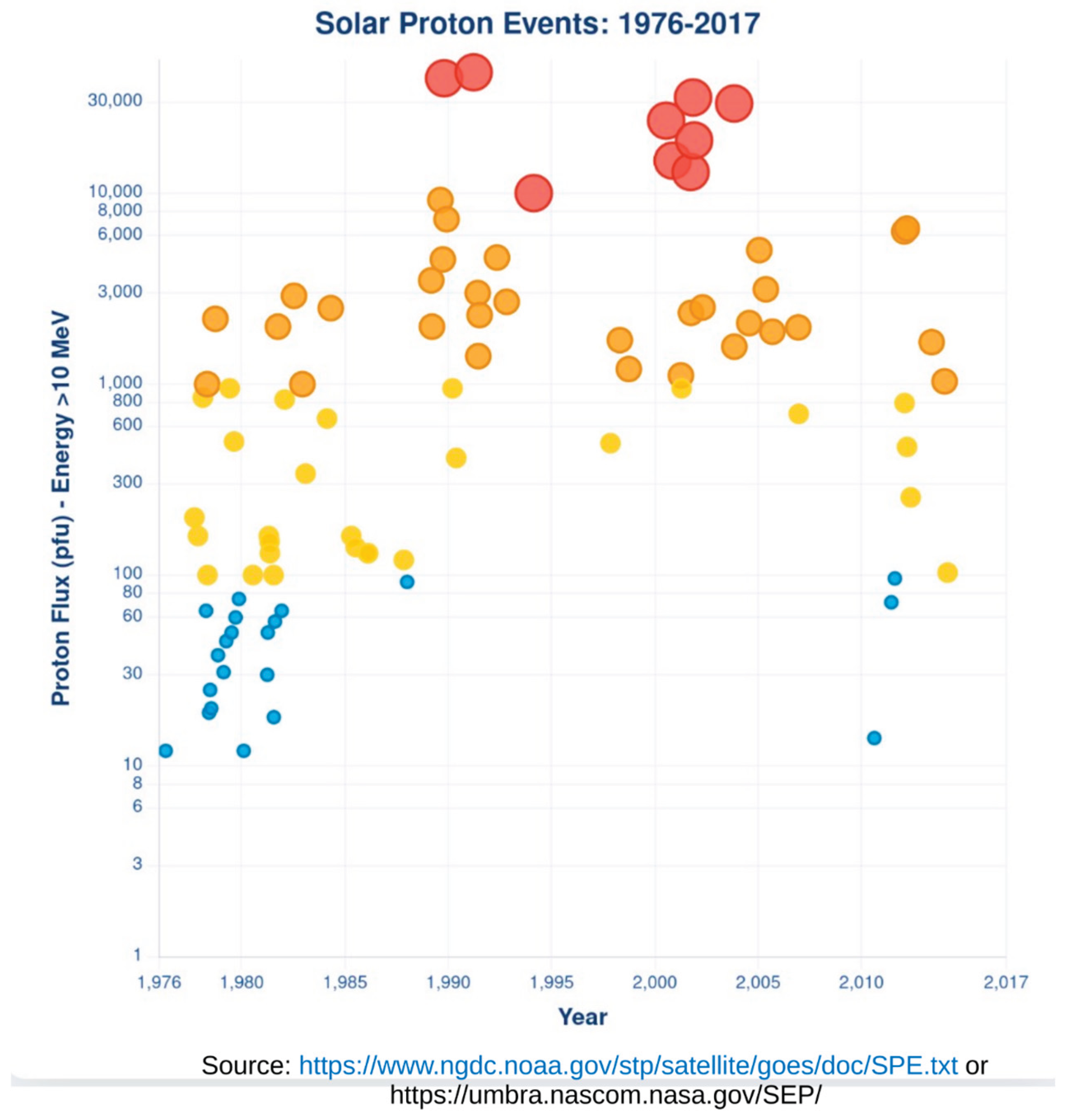
As shown in Figure 3, there were two periods of unusual solar activity involving increased proton flux just before and sometime after the eruption of Pinatubo. Solar activity has been shown to have an effect on atmospheric water vapor by Galkin et al., [16]. A plot of solar proton activity is shown in Figure 4. However these events are not expected to have a long lasting effect on reducing water vapor.

Water Vapor from Jet Airplanes

The claim is that aircraft produce 10 trillion cubic feet of water vapor annually because for every pound of jet fuel burned a pound of water is produced, https://artificialclouds.com/ . Others estimate 1.231 pounds of water per pound of fuel [17,18,19].

The Vonnegut Climate Change Theory (Dr. Bernard Vonnegut) is described in a sequence of steps at the above link. Step 6 indicates:

The trillions of cubic feet of frozen water vapor created by jet aircraft every year (mostly in the northern hemisphere) is in the form of expanding gaseous clouds of microcrystals which continue to rise from the lower stratosphere, collecting and building up in the mesosphere.

Recent estimates of jet fuel use correspond to one day’s worth of global aviation industry demand of 336 million gal/day or 122 billion gallons per year, https://www.opis.com/blog/2025-likely-to-bring-lower-jet-fuel-prices-higher-demand/ . This would correspond to 1.231*122 = 150 billion gallons of water or 568 Tg of water. Tonga-Hunga is estimated to have ejected 150 Tg of water vapor into the upper atmosphere. So these aircraft are injecting about 3.8 times as much water into the atmosphere as Tonga-Hunga. This happens over a year rather than over a couple of weeks. However aircraft travel year round so this is a sustained injection of water vapor. Does this sustained injection of water vapor lead to higher sustained atmospheric water vapor or does it all condense out of the atmosphere? Estimates indicate that only a few percent of anthropogenic radiative forcing is due to aviation [17] suggesting that the water vapor is assumed to condense out of the atmosphere.

Climate Models and Glacial Inception

The Earth’s climate is extremely complex. The only way to attempt to understand the climate is to model the climate using the best understanding available and test predictions with measurements. A problem that immediately arises has to do with time scale. According to the World Meteorological Organization (WMO), Background [20]:

The general recommendation is to use 30-year periods of reference. The 30-year period of reference was set as a standard mainly because only 30 years of data were available for summarization when the recommendation was first made.

This indicates that the 30 year averaging period often used to define “climate” data was forced rather than scientifically defined. So there may be a problem with the standard definition of a “climate” value for a given measured variable.

Climate models, at least those that try, seem to have difficulty making the transition from an interglacial to a glacial period. For example [21]:

Fifth, CCSM4 has a cold bias in northern Canada and northern Siberia41 that predisposes the model toward forming permanent snow cover in a cooler climate. However, these are mostly cold-season biases36; in spring-summer, the terrestrial cold bias is smaller, while the Canadian Archipelago even has a weak warm bias42. Nevertheless, the model produces too much snow cover in its 20th century transient simulation over Alaska, the Rocky Mountains, and much of northern Canada (including Baffin), which are glacial inception regions in the model42.

Another example [22]:

This allows for the to artificial acceleration of the external forcings, in this case orbital parameters and GHGs concentration, which, considering that the atmosphere and ocean are also the most computationally expensive parts of an Earth system model results in an effective speed-up of the model.

The glacial inception simulations presented here are a first step towards simulating the full last glacial cycle with CLIMBER-X.

Until climate models can match the prior interglacial into glacial inception and rise out of that glacial into the current interglacial, models are still in the development phase and should be used with considerable caution to predict future climate attributes.

Discussion

The Earth climate is complex so the only way to determine if the climate is understood is through modeling. However, a climate model that is driven by rising CO2 stimulating rising water vapor and thereby rising temperature would have difficulty modeling the interglacial of 127,000 BCE to 114,000 BCE because temperature was falling while CO2 remained high and constant.

Influences that might account for Figure 1 cooling while CO2 remained high and constant that have been considered are: ice sheet growth, ocean current change, clouds, volcanic eruptions, meteor or comet impacts, and solar activity. Among these, clouds and solar activity remain as possible and most reasonable explanations primarily because they cannot be discounted due to lack of available data for the time interval involved. However, using either cloud variation or solar variation as an explanation for the cooling immediately discounts the argument that CO2 is the undoubted major climate driver of the prior interglacial period.

Is it possible that orbital cycles induce initial warming, initial warming induces increased sustained water vapor and increased CO2, with sustained water vapor being the primary cause of rising temperature. As temperature rises and sustained water vapor rises perhaps cloud cover that would lower temperature initially holds roughly constant – maybe rising CO2 is responsible ( https://www.caltech.edu/about/news/high-cosub2sub-levels-can-destabilize-marine-layer-clouds#:~:text=High%20CO2%20Levels%20Can%20Destabilize,Environment%20%2D%20www.caltech.edu ). Suppose glacial inception occurs because at some point rising sustained water vapor triggers clouds that cool even in the presence of higher atmospheric CO2. This would mark the high temperature of the last interglacial. From that point forward clouds continue to lower the temperature. Perhaps once water vapor has triggered cooling cloud cover it becomes persistent even if sustained water vapor is lowered. CO2 remains high because it is dispersed evenly throughout the atmosphere and requires a long interval of time to approach the ocean surface and be absorbed. The problem with this conjecture is: (1) can rising sustained water vapor generate cooling clouds, and (2) can cooling clouds be persistent once formed while allowing water vapor to be lowered?

Current variations in water vapor measurements may reasonably be assumed to be due to volcanic eruptions with VEI above 4 – inserting noise, unrelated to climate, into the water vapor atmospheric concentration. These eruptions can eject water vapor very high into the atmosphere where ice crystals are formed and condensation is inhibited in favor of sublimation. If the eruption is strong enough to inject very large amounts of water vapor into very high elevations as ice crystals, the equilibrium of atmospheric water vapor in the upper atmosphere may be raised to a higher level “quasi equilibrium” that slowly decreases unless another massive volcanic eruptions injects more water vapor into high elevations.

One also wonders if all the water vapor, injected into the atmosphere by jet aircraft, really does condense out and can therefore be discounted as a source of sustained high atmospheric water vapor.

These possible conjectures and questions are offered to stimulate critical thought, conversation, and further research into understanding our complex climate.

Funding

This research received no external funding.

Conflicts of Interest

The author declares no conflicts of interest.

References

Earle S. Physical Geology. 2nd ed. Victoria BC, editor. British Columbia: B C campus; 2019.
Jouzel, J., et al. 2007. EPICA Dome C Ice Core 800KYr Deuterium Data and Temperature Estimates. IGBP PAGES/World Data Center for Paleoclimatology Data Contribution Series # 2007-091. NOAA/NCDC Paleoclimatology Program, Boulder CO, USA.
Bereiter, B.; Eggleston, S.; Schmitt, J.; Nehrbass-Ahles, C.; Stocker, T.F.; Fischer, H.; Kipfstuhl, S.; Chappellaz, J, Antarctic Ice Cores Revised 800KYr CO2 Data, Contribution date: 2015-02-04, World Data Center for Paleoclimatology, Boulder and NOAA Paleoclimatology Program.
Maslin, M., M. Sarnthein, J. J. Knaack, Subtropical Eastern Atlantic Climate During the Eemian, (1996), Naturwissenschaften, Spring-Verlag.
Hodell, David A., Emily Kay Minth, Jason H. Curtis, I. Nicholas McCave, Ian R. Hall, James E.T. Channell, Chuang Xuan, Surface and deep-water hydrography on Gardar Drift (Iceland Basin) during the last interglacial period, (2009), Earth and Planetary Science Letters,. [CrossRef]
Jakob, Christian, edited by Gaby Clark, reviewed by Andrew Zinin, Global warming is changing cloud pattrens. That means more global warming, The Conversation, Phys.org, https://phys.org/news/2025-06-global-cloud-patterns.html.
S.D. Burgess, J.A. Vazquez, C.F. Waythomas, K.L. Wallace, U–Pb zircon eruption age of the Old Crow tephra and review of extant age constraints, Quaternary Geochronology, Volume 66, 2021, 101168, ISSN 1871-1014, (https://www.sciencedirect.com/science/article/pii/S1871101421000194). [CrossRef]
Dee, Michael, Andrea Scifo , Tarun Rohra, Jente Joosten, Margot Kuitems , Wesley Vos, Sturt Manning and Thorsten Westphal, Radiocarbon evidence over the apparent grand solar minimum around 400 BCE, Radiocarbon (2025), 67, pp. 265–274, Cambridge University Press. [CrossRef]
van Wijngaarden, W. A. and W. Happer, Dependence of Earth’s Thermal Radiation on Five Most Abundant Greenhouse Gases, arXiv:2006.03098v1 [physics.ao-ph] 4 Jun 2020.
de Lange C. A. , J. D. Ferguson , W. Happer , and W. A. van Wijngaarden, Nitrous Oxide and Climate, arXiv:2211.15780v1 [physics.ao-ph] 28 Nov 2022.
van Wijngaarden W. A. and W. Happer, The Role of Greenhouse Gases in Energy Transfer in the Earth’s Atmosphere, arXiv:2303.00808v1 [physics.ao-ph] 1 March 2023.
Findell, Krsten L., Patrick W. Keys, Ruud J. van der Ent, Benjamin R. Lintner, Alexis Berg, and John P. Krasting, Rising Temperatures Increase Importance of Oceanic Evaporation as a Source for Continental Precipitation, (2019), American Meteorological Society. [CrossRef]
Ashera, Elizabeth , Michael Todta, , Karen Rosenlof , Troy Thornberry, Ru- Shan Gao , Ghassan Tahac, , Paul Walter , Sergio Alvarez, James Flynn , Sean M. Davis, Stephanie Evan , Jerome Brioude , Jean- Marc Metzger , Dale F. Hurst, Emrys Hall, and Kensy Xiong, Edited by Mark Thiemens, Unexpectedly rapid aerosol formation in the Hunga Tonga plume, 2023, PNAS research article | Earth, Atmospheric, and Planetary Sciences. [CrossRef]
Chen, Xi, Jun Wang, Meng Zhou , Zhendong Lu, Lyatt Jaegle , Luke D. Oman & Ghassan Taha, Impact of water vapor on stratospheric temperature after the 2022 Hunga Tonga eruption: direct radiative cooling versus indirect warming by facilitating large particle formation, (2025), npj | climate and atmospheric science. [CrossRef]
Gupta, Ashok Kumar, Tushar Mittal, Kristen E. Fauria, Ralf Bennartz & Jasper F. Kok, The January 2022 Hunga eruption cooled the southern hemisphere in 2022 and 2023, (2025), communications earth & environment, A Nature Portfolio journal. [CrossRef]
Galkin, V.D., Nikanorova, I.N. Solar activity and atmospheric water vapor. Geomagn. Aeron. 55, 1175–1179 (2015). [CrossRef]
Lee, D.S.,D.W. Fahey, A. Skowron, M.R. Allen, U. Burkhardt, Q. Chen, S.J. Doherty, S. Freeman, P.M. Forster, J. Fuglestvedt, A. Gettelman, R.R. De Le´on, L.L. Lim, M. T. Lund, R.J. Millar B. Owen, J.E. Penner, G. Pitari, M.J. Prather, R. Sausen, L. J. Wilcox, The contribution of global aviation to anthropogenic climate forcing for 2000 to 2018, (2021), Atmospheric Environment. [CrossRef]
S. Barrett, M. Prather, J. Penner, H. Selkirk, S. Balasubramanian, A. Dopelheuer, G. Fleming, M. Gupta, R. Halthore, J. Hileman, M. Jacobson, S. Kuhn, S. Lukachko, R. Miake-Lye, A. Petzold, C. Roof, M. Schaefer, U. Schumann, I. Waitz, R. Wayson, Guidance on the Use of AEDT Gridded Aircraft Emissions in Atmospheric Models, Massachusetts Institute for Technology, Laboratory for Aviation and the Environment (2010), https://citeseerx.ist.psu.edu/document?repid=rep1&type=pdf&doi=aae3bd04f264b1d0d584c5480e3b31d70fb92c39.
Leron Wells, (2023) personal communication at Walker Water LLC.
WMO Guidelines on Calculation of Climate Normals, 1017 edition, World Meteorological Organization, Chairperson, Publications Board, World Meteorological Organization (WMO), 7 bis, avenue de la Paix, P.O. Box 2300, CH-1211 Geneva 2, Switzerland, Tel.: +41 (0) 22 730 84 03, Email: publications@wmo.int, ISBN 978-92-63-11203-3.
Vavrus, Stephen J., Feng He, John E. Kutzbach, William F. Ruddiman & Polychronis C. Tzedakis, Glacial Inception in Marine Isotope Stage 19: An Orbital Analog for a Natural Holocene Climate, (2018), Scientific Reports. [CrossRef]
Willeit, Matteo, Reinhard Calov, Stefanie Talento, Ralf Greve, Jorjo Bernales, Volker Klemann, Meike Bagge, and Andrey Ganopolski, Glacial inception through rapid ice area increase driven by albedo and vegetation feedbacks, (2024), Climate of the Past, Published by Copernicus Publications on behalf of the European Geosciences Union. [CrossRef]

Figure 1. During the prior interglacial, temperature reached a maximum and atmospheric CO2 peaked. Then CO2 remained constant for 13,000 years while temperature fell 7 to 8 degrees C. Data was sourced from [2,3] with no smoothing applied. For the interval shown the maximum sigma mean for CO2 is 6.56 ppm for one point with most showing 2.65 ppm, while for temperature optimal accuracy ± 0.5 ‰ (1 sigma) .

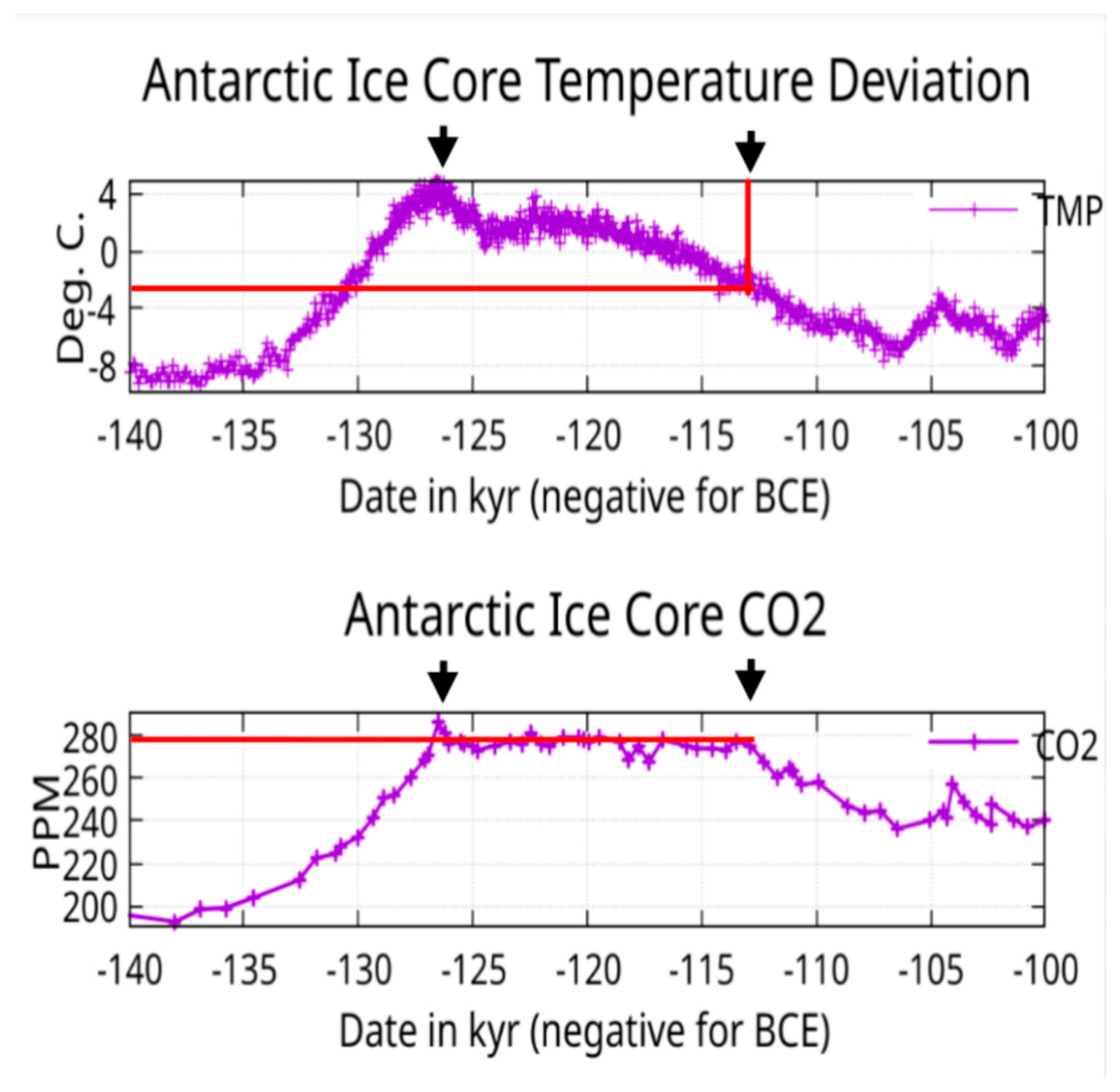
Figure 2. Stratospheric water vapor mixing ratios measured by the balloon-borne NOAA Frost Point Hygrometer (FPH) over Boulder, Colorado. Data are averaged in 2-km altitude bins. The long-term net increase through 2013 is approximately 20%. Plot created by Dale Hurst (dale.hurst@noaa.gov). This figure was found at https://gml.noaa.gov/ozwv/wvap/ of NOAA’s Global Monitoring Laboratory.

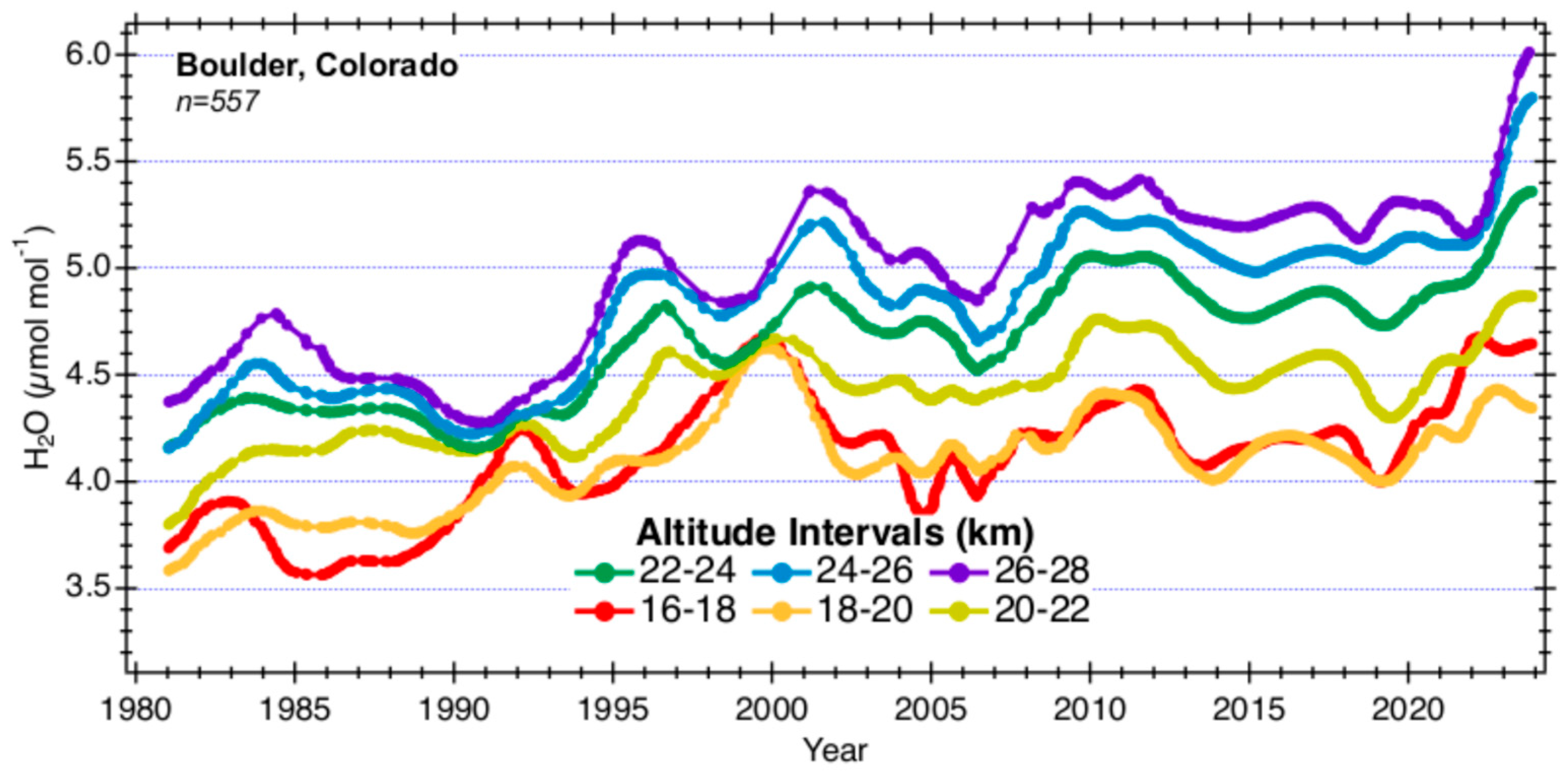
Figure 3. In this version of the figure volcanic eruptions with Volcanic Explosivity Index (VEI) of 4 or higher are indicated with those above VEI 4 shown along the top. An increase of 1 index indicates an eruption that is 10 times as powerful. Periods of unusual solar activity (Proton Flux) have also been indicated. A connected straight line indicates an alternate trend interpretation with four associated time intervals: A, B, C and D indicated.

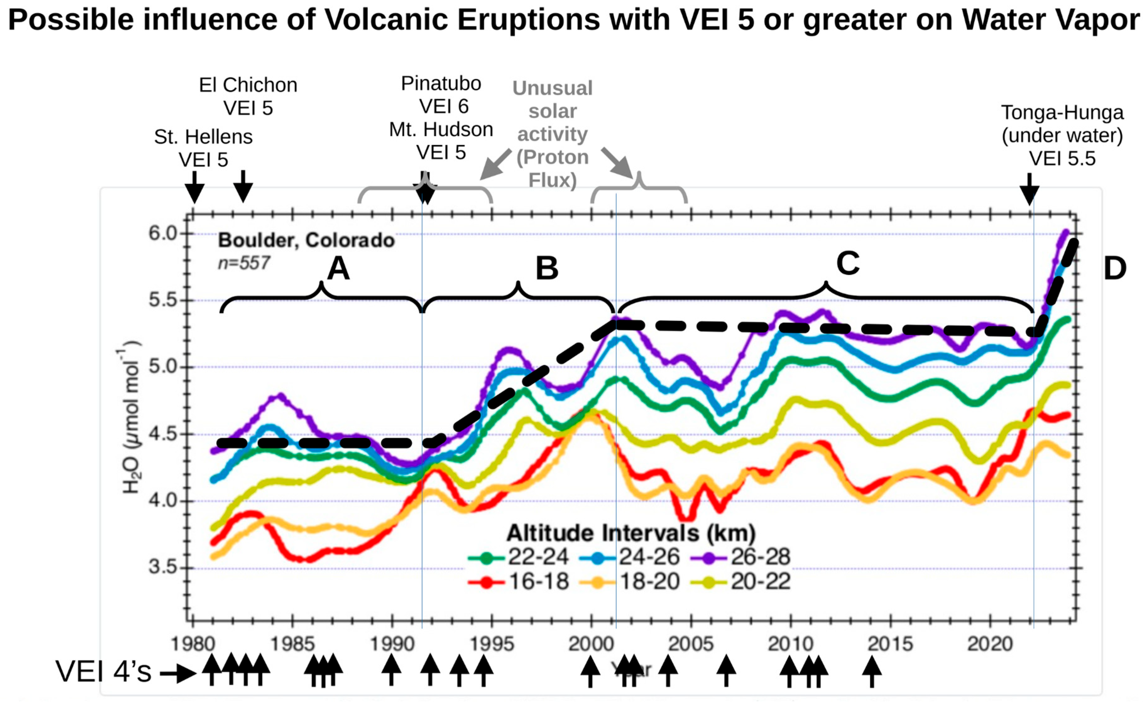
Figure 4. Solar Proton Events: Plot generated from data at https://www.ngdc.noaa.gov/stp/satellite/goes/doc/SPE.txt.

Disclaimer/Publisher’s Note: The statements, opinions and data contained in all publications are solely those of the individual author(s) and contributor(s) and not of MDPI and/or the editor(s). MDPI and/or the editor(s) disclaim responsibility for any injury to people or property resulting from any ideas, methods, instructions or products referred to in the content.

© 2025 by the authors. Licensee MDPI, Basel, Switzerland. This article is an open access article distributed under the terms and conditions of the Creative Commons Attribution (CC BY) license (http://creativecommons.org/licenses/by/4.0/).

Copyright: This open access article is published under a Creative Commons CC BY 4.0 license, which permit the free download, distribution, and reuse, provided that the author and preprint are cited in any reuse.