
Submitted:
27 August 2025
Posted:
28 August 2025
You are already at the latest version
Abstract
Crested Wheatgrass (Agropyron cristatum) is an introduced invasive grass species in North American grasslands. It was initially seeded to increase the grazing duration, but is now threatening native grassland biodiversity. Effective monitoring of Crested Wheat-grass requires robust remote sensing methods, yet prior studies relying on multispectral satellite data have faced limitations due to spectral similarity with co-occurring vegetation. In this study, we investigated which biophysical and spectral properties (hyperspectral and simulated multispectral) distinguish Crested Wheatgrass from native grasses. We further assessed whether spectral indices, linked to biophysical traits, could distinguish Crested Wheatgrass from native grasses. We collected field data of hyperspectral reflectance, leaf area index (LAI), biomass, and vegetation cover. We found that the differences between Creased Wheatgrass and native grasses are significant for many biophysical properties and spectral features. Grass cover, height, LAI, and biomass (grass, total and dead) are much higher for Crested Wheat grass sites, while bare ground cover is lower compared to native grasses. Hyperspectral data revealed distinct lower reflectance for Crested Wheat grass in visible and shortwave infrared regions (SWIR) compared to native grasses, which might be driven by differences in photosynthetic pigments and moisture content. SWIR spectral indices for hyperspectral data, SWIR and visible spectral indices for simulated Sentinel-2A data, and visible spectral indices for PlanetScope SuperDove data discriminated Crested Wheatgrass from native grasses. These findings advance invasive grass monitoring by shifting the focus from phenology to biophysical properties based detection, supporting management of Crested Wheatgrass and restoration of native grassland ecosystems.
Keywords:
Crested Wheatgrass
; Hyperspectral remote sensing
; Invasive grass
; Spectral indices
; Simulated multispectral data
1. Introduction
Crested Wheatgrass (Agropyron cristatum), an introduced invasive species, is responsible for the degradation of the native grassland ecosystem in the Great Plains of North America [1,2,3,4]. It was mainly introduced for the revegetation of degraded rangelands and farmlands following severe drought years during the 1930s [5,6]. It was ideal for this purpose because of its establishment success, resilience to adverse environmental conditions and grazing tolerance [7]. Crested Wheatgrass can establish in an area with low water availability, quickly stabilizes bare soil and it can produce 1.5 to 2 times more forage than native stands [8]. Due to its competitiveness, it hampers the establishment of other invasive species such as Downy Brome [5]. Additionally, Crested Wheatgrass is considered good forage for cattle as it greens up early in the spring [9] facilitating its use for early spring grazing [10]. Urness et al. [11] reported that Crested Wheatgrass is also suitable forage for wildlife such as mule deer.
Despite these benefits it presents some ecological challenges. It reduces plant diversity by hampering the establishment and persistence of native plant species, resulting in a monoculture [12,13,14,15]. Available soil moisture beneath Crested Wheatgrass stands is lower than native species mainly because of its high rate of water usage [12,16]. Moreover, Crested Wheatgrass has a lower root-shoot ratio compared to native plants, leading to a low below-ground carbon storage [3,12]. Crested wheatgrass also affects the abundance of fauna species in an ecosystem. For instance, [17] reported that Crested Wheatgrass presence negatively influenced the abundance of grassland bird species.
To fully harness the potential benefits of an introduced invasive species, such as Crested Wheatgrass, in a native grassland ecosystem, proper management strategies must be implemented, beginning with the effective monitoring of their spatial distribution. Remote sensing can be an effective means to monitor whether an introduced invasive species is spreading beyond its designated area, and it can be used to assess the effectiveness of management practices, such as mowing, prescribed burning, or herbicide application in controlling or eradicating the species. Remote sensing can be successfully used in invasive species mapping given that the invasive species has distinct phenological patterns compared to surrounding native vegetation, unique plant traits, and widespread distribution in the study area [18,19]. Some invasive species, such as Crested Wheatgrass, may exhibit overlapping phenological patterns with other invasive species, such as Smooth Brome. Also, the timing of these phenophases might change with environmental conditions. In both of these cases, distinct biophysical or biochemical plant traits of invasive species can be leveraged to enhance the accuracy of remote detection [19]. Spatial and spectral resolution of remote sensing datasets should also be considered to detect invasive plant species of varying patch sizes and traits [18,20]. Specifically, high spatial (e.g., airborne remote sensing) and spectral resolution (e.g., hyperspectral remote sensing) data is a must to accurately detect an invasive plant at the species level [18,21,22].
In terms of Crested Wheatgrass, time and labor-intensive field monitoring approaches (e.g., marker demarcation, plant counting, ground cover photography) are still being suggested [23]. Only a few studies have tried to detect Crested Wheatgrass using remote sensing. Weidong [24] used different vegetation indices on a single date (27 July 2006) SPOT-5 image to separate Crested Wheatgrass from the native vegetation. However, it was concluded that the accuracy of the classification was not satisfactory due to the spectral similarity of the two vegetation types. Guo et al. [25] mapped the spatial distribution of Crested Wheatgrass using visible and shortwave infrared bands of Sentinel-2A data with 70% overall accuracy and concluded that using a higher spatial resolution might result in a more accurate detection of Crested Wheatgrass. Similarly, Weisberg et al. [22] mapped the distribution of several invasive species, including Crested Wheatgrass, using five bands (Blue, Green, Red, Red Edge and NIR) collected using a multispectral sensor mounted on an unmanned aerial vehicle, collected during the growing seasons (May - July). However, in this phenology-based classification approach, the distribution of Crested Wheatgrass was greatly confounded with other vegetation types, highlighting a research gap where higher spectral resolution could also be explored to achieve improved classification results.
Based on our knowledge, there is a lack of studies that have examined the unique biophysical properties of Crested Wheatgrass, which can help us understand what drives the invasiveness of Crested Wheatgrass. Moreover, previous studies suggest insufficient understanding of the spectral characteristics of Crested Wheatgrass that are essential for its precise detection [24,25]. Proximal remote sensing sensors such as field spectroradiometers, unaffected by atmospheric interference, provide precise spectral profiles that are critical for distinguishing invasive species from others. This initial step is vital for selecting appropriate remote sensing approaches and enhancing the accuracy of satellite detection. Separating Crested Wheatgrass by integrating plant traits and spectral information can also help bridge the current research gap, shifting the focus from phenological indicators to plant trait based remote detection of invasive species. Therefore, the overall purpose of this research is to detect Crested Wheatgrass using field-based hyperspectral remote sensing. Specifically, the objectives are (1) to identify the unique biophysical and spectral characteristics of Crested Wheatgrass and native grasses using both hyperspectral and simulated multispectral data, and (2) to differentiate Crested Wheatgrass based on the relationships between spectral indices and biophysical properties.
2. Materials and Methods
2.1. Study Area
Saskatchewan Landing Provincial Park (SLPP) (50° 39′ 58″ N, 107° 59′ 23″ W) is situated in the Southwest of the Saskatchewan Province and along the South Saskatchewan River, Canada [26] (Figure 1). This provincial park was established in 1973, and being one of the largest provincial parks in the native prairie region, it encompasses an area of about 57.35 km2 [25]. SLPP belongs to the Mixed-Grass Prairie ecoregion [27] and is a unique habitat for a number of different flora and fauna species [25]. The topography of the park was shaped by de-glaciation, and the elevation of this area ranges from 554 m to 708 m, with varying levels of steepness (0% - 92%) [25]. Between 2000 to 2022, the average annual precipitation was 365.62 mm and the average daily temperature was 4.7oC [28]. Loamy soil predominates in this region while a small portion of the area is characterized by clay [25]. The distribution of vegetation communities in the park varies according to topography and soil types [29]. Some of the dominant native grassincludes spear grasses (Hesperostipa comata, Nassella viridula), blue grama grass (Bouteloua gracilis), western wheatgrass (Pascopyron smithii), and slender wheatgrass (Elymus trachycaulus) (Tremblay, 2013). Sage brush (Artemisia tridentata), hybrid cottonwood (Populus x jackii), Manitoba maple (Acer negundo), Trembling aspen (Populus tremuloides), Chokecherry (Prunus virginiana), Rose (Rosa spp.) and Creeping juniper (Juniperus horizontalis) are some of the shrub species found in SLPP [25]. Among the exotic species, Crested Wheatgrass (Agropyron cristatum) is the most dominant in SLPP with some dispersion of Smooth brome (Bromus inermis) and Kentucky blue grass (Poa pratensis) [25,30]. Moreover, there are different noxious weeds, including Russian knapweed (Rhaponticum repens), Canada thistle (Cirsium arvense), leafy spurge (Euphorbia esula), kochia (Kochia scoparia) and common buckthorn (Rhamnus catharticus) [25].
2.2. Field Data Collection
Field data was collected in late May 2024, when Crested Wheatgrass typically matures, due to its early spring (late April or early May) growth initiation [9]. This phenological difference with other vegetation may result in higher phenological differentiation during this time. A total of 21 sites were selected; 13 sites were situated in Crested Wheatgrass dominant locations and 8 were in native grass dominated ones. In order to determine Crested Wheatgrass and native grass dominated sites, species composition and grass cover threshold percentage were used as criteria. If the site has more than 50% coverage, of total vegetation cover, of a grass species (Crested Wheatgrass or native grass), the site is considered to be dominated by that species. Within each site, two 20 m transects perpendicular to each other were used to collect hyperspectral and biophysical measurements with 50 cm X 50 cm quadrats (referred to as Q(5m,10m) quadrat) along the transects at 5 m intervals (Figure 2). Within each of these quadrats, hyperspectral reflectance, cover percentage of different functional vegetation groups (grass, shrub, forbs, standing dead, litter and bare ground), grass and shrub height (maximum), and leaf area index (LAI) were recorded. Lastly, GPS coordinates of the transect intersection point where collected using a Geo XH 2008 Series Geo Explorer GPS.
Cover estimation followed the approach used by [34]. When the fractional cover was larger than 5% and smaller than 95%, it was estimated at a 5% increments. When it was below 5% and over 95%, it was estimated at a 1% increment. LAI was measured using a Li-COR LAI-2000, with one above-canopy and five below-canopy measurements, as this sampling intensity was sufficient for accurate site wise LAI calculation [35]. The average LAI from 8 quadrats was calculated to represent the LAI value for the site. A Spectroradiometer (ASD FieldSpec Pro) was used to collect field hyperspectral data. This spectroradiometer captures a broad range of wavelengths (350 nm to 2500 nm) that are covered by the visible, shortwave infrared 1 (SWIR1), and shortwave infrared 2 (SWIR2) detectors. It comes with a high spectral resolution of 3nm within the 350 nm to 1000 nm range and 10 nm at the 1000 nm to 2500nm range. During field data collection, the spectrometer was held 1 m above ground to record the spectral data from each quadrat with the field of view (FOV) of 25o. The measurements were taken from 10 am to 2 pm during clear sky conditions and with the operator facing the sun to avoid any shadow on the quadrats. A digital picture of each of these 8 quadrats was taken using a digital camera at nadir view.
Above ground biomass harvesting was conducted for four quadrats (Q(5m)) of size 20 cm x 50 cm at each site [36,37]. All the vegetation was cut, bagged, and weighed. Sorting took place in the lab to separate green grass, green forb, green shrub, and dead materials. All samples were then dried to weight the dry biomass. All the data (spectral, biomass, vegetation cover, LAI, height) from the Q(5m,10m) and Q(5m) quadrats were averaged to represent the values in their respective sites.
2.3. Data Analysis
2.3.1. Biophysical Properties
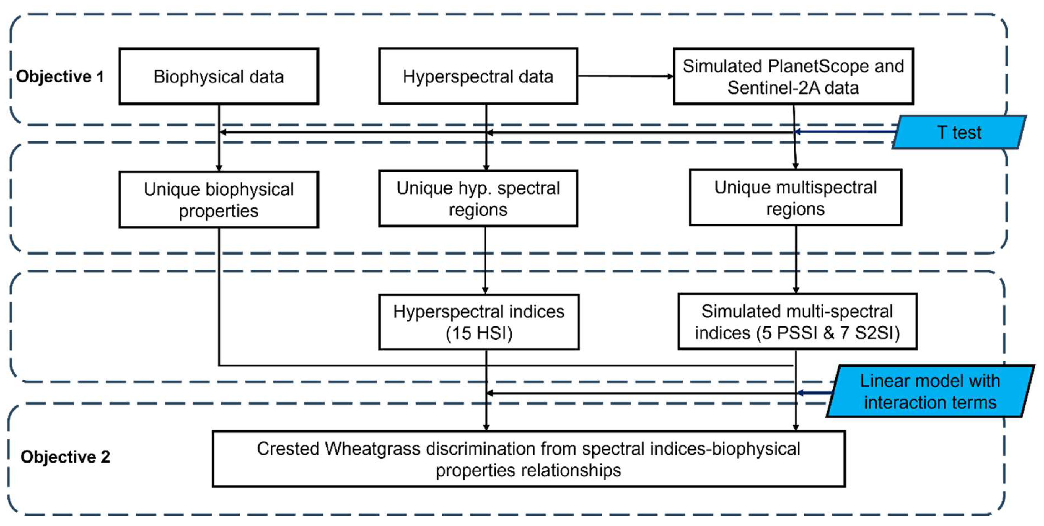
A Weltch T test [38] was conducted to investigate the difference between the biophysical properties of Crested Wheatgrass and native grass for 11 biophysical properties – cover (green grass, standing dead, litter, bare ground, shrub), height, LAI, biomass (green grass, total, dead, and shrub). The biophysical properties that were significantly different were used later during spectral discrimination.
Figure 3.
summarizes the study workflow used in this study, from biophysical and spectral data collection to Crested Wheatgrass discrimination using linear models.
Figure 3.
summarizes the study workflow used in this study, from biophysical and spectral data collection to Crested Wheatgrass discrimination using linear models.
2.3.2. Remote Sensing Dataset
The water absorption bands (1350–1430 nm, 1750–1980 nm, and 2330– 2500 nm) were removed as a pre-processing step [39] of the field hyperspectral data. Then, the hyperspectral data were resampled to two multispectral sensors (PlanetScope SuperDove and Sentinel 2A) using their spectral response function information [40,41] to evaluate the potential application of satellite imagery in discriminating Crested Wheatgrass. The following formula was used in the resampling process which was adapted from Zheng et al. [42]:
Where, R is the resampled reflectance of a band of a multispectral sensor, λend and λstart represents end and start of wavelength of a band respectively, and f(x) is the spectral response of the multispectral sensor.
Welch’s t-test was applied to identify spectral regions where reflectance significantly differed (p < 0.05) between Crested Wheatgrass and native grass for the hyperspectral and simulated data. Then, using these significant spectral regions, hyperspectral and simulated multispectral vegetation indices were computed to further assess grass species discrimination (Table 1).
2.3.3. Linear Model with Interaction Effect
Initial assessments of biophysical properties and spectral indices using a linear model indicated interactions between Crested Wheatgrass and native grass across multiple response variables. Therefore, a linear model with interaction effects was applied separately to each of the significant biophysical properties and spectral indices (both hyperspectral and simulated multispectral) combinations. The model assessed whether the relationship between spectral indices (SI) and biophysical properties (BP) varied significantly between species (Crested Wheatgrass and native grass), with BP as the response variable, species type, SI and their interaction term (species type × SI) as the independent variables for species-wise effects. While the primary goal of using linear model to identify SI and BP associations with significant species-wise differences, we also examined the strength of the associations by analyzing the slope coefficients of the final models.
3. Results
3.1. Biophysical Properties of Different Grassland Types
Several biophysical properties are significantly different between Crested Wheatgrass and native grass including grass and bare ground cover, height, LAI, and biomass (grass, total, and dead) (p <0.05) (Table 2). Except for bare ground cover, all the other biophysical properties were significantly higher for Crested Wheatgrass. Coefficient variation assessment indicated that Crested Wheatgrass had lower spatial variation for most of the biophysical variables (Table 2).
3.2. Spectral Properties of Different Grassland Types
Native grass had higher spectral reflectance compared to Crested Wheatgrass in the visible, shortwave infrared (SWIR), and some parts of the NIR region (Figure 4), according to the hyperspectral data. Statistical results showed that Crested Wheatgrass and native grass had significantly different spectral reflectance in the visible (390-700 nm) and the SWIR (1430-1749 nm and 1981-2329 nm) regions (p <0.05) (Figure 4). Based on these unique hyperspectral regions, 15 hyperspectral indices were calculated (Table 1) to represent different biophysical properties.
The simulated Sentinel-2A and PlanetScope SuperDove spectral data showed the same patterns as the hyperspectral data (Figure 5). Reflectance in the coastal blue and visible (blue, green I, green II, red and yellow) bands differed significantly between Crested Wheatgrass and native grass (p < .05) for simulated PlanetScope SuperDove data (Figure 5). For simulated Sentinel-2A, the coastal aerosol, visible (blue, green and red) and shortwave infrared (SWIR1 and SWIR 2) bands showed noticeable differences in reflectance between the two grass types (p <0.05) (Figure 5). Using the significant bands, five simulated PlanetScope SuperDove spectral indices and seven simulated Sentinel-2A indices (Table 1) were calculated, all of which (except for one Sentinel-2A index: Hyperspectral biomass and structural index) were adapted from the calculated hyperspectral indices.
3.3. Crested Wheatgrass Discrimination Using a Linear Model with Interaction
Clear interactions can be observed when estimating biophysical properties using spectral data for Crested Wheatgrass and native grass (Figure 6) using hyperspectral indices. We selected those with the strongest species-specific pattern (lowest p-value for the species type × SI interaction term) for the relationship between biophysical properties and spectral indices (Table 3). The Height–Shortwave Vegetation Index (SWVI) (pint = 0.005), Grass biomass–Cellulose Absorption Index (CAI) (pint = 0.002), Total biomass–CAI (pint = 0.021), and Leaf area index–CAI (pint = 0.003) model showed a negative association between biophysical properties and spectral indices for Crested Wheatgrass, while opposite pattern was observed for native grass. However, in the Bare ground cover–CAI (pint = 0.007) model, Crested Wheatgrass and native grass showed opposing patterns compared to the other four models (Figure 6 and Table 3).
Similar interactions were revealed using the simulated PlanetScope SuperDove indices (Figure 7 and Table 3). In the Grass cover–Photochemical reflectance index PlanetScope SuperDove (PRIPS) (pint = 0.007), LAI–Red green ratio PlanetScope SuperDove (RGRPS) (pint = 0.028) and Total biomass–RGRPS (pint = 0.019) models, the biophysical properties of Crested Wheatgrass were inversely associated with the spectral indices, contrasting with the positive association observed in native grass (Figure 7 and Table 3). For the Grass cover–PRIPS and LAI–RGRPS (pint = 0.028) model, biophysical properties of native grasses showed minimal response to variations in spectral indices (Figure 7). However, for the Bare ground cover-RGRPS model, bare ground in Crested Wheatgrass plots increased with RGRPS values, whereas native grasses showed a negative trend (Figure 7 and Table 3).
Similarly, using the simulated Sentinel-2A spectral indices, three linear models stood out as having the strongest species-wise pattern (Table 3). The total biomass and LAI values decreased with the respective spectral index values for Crested Wheatgrass in the Total biomass-Red green ratio Sentienl-2A (RGRS2) and Leaf area index-Red green ratio Sentienl-2A (RGRS2) model respectively (Figure 8 and Table 3). But total biomass showed positive association with RGRS2 for native grass and LAI remained constant (Figure 8 and Table 3). Conversely, the Bare ground cover- Water stress index (WSI) models revealed opposing patterns for Crested Wheatgrass and native grass compared to the first two models (Figure 8 and Table 3).
4. Discussion
Several studies have combined plant biophysical properties with spectral signatures to discriminate invasive vegetation species (Gholizadeh et al., 2022; Mallmann et al., 2023; Rakotoarivony et al., 2023). Building on this approach, this study identified unique biophysical and spectral characteristics of Crested Wheatgrass using hyperspectral data and simulated multispectral data and related these variables to effectively distinguish Crested Wheatgrass from native vegetation.
4.1. Biophysical Differences Explain Crested Wheatgrass Dominance
We found that 7 biophysical properties showed significant differences between the two grass type groups (Table 2). Except for the bare ground cover, all the biophysical properties are higher for Crested Wheatgrass. These results could provide an understanding of which biophysical properties facilitate competition, establishment, and spread mechanisms of Crested Wheatgrass. For instance, the tall and dense structure of Crested Wheatgrass might hamper the establishment of other surrounding vegetation that are shade intolerant, which in turn may lead to high dominance of Crested Wheatgrass and low diversity in the stand [58]. Further, this tall stature of Crested Wheatgrass may help it to capture more light, thus leading to higher overall biomass and leaf area construction [59,60,61]. This also substantiates the result that we found for the higher biomass and LAI of Crested Wheatgrass in this study (Table 1). Christian and Wilson [3] and Nafus er al. [62] observed a similar result showing that Crested Wheatgrass had a higher abundance compared to other vegetation. However, Davies et al. [63] found that Crested Wheatgrass abundance did not significantly increase after a seven-year period compared to other vegetation cover. This high density and cover of Crested Wheatgrass can also be used to explain the bare ground cover result found in this study. Henderson [64] reported a relationship between the presence of Crested Wheatgrass and bare ground cover, noting that the removal of Crested Wheatgrass led to an increase in bare ground. However, it depended on the site-specific conditions. In our case, the dryness of native grass areas and factors such as age or poor establishment of Crested Wheatgrass may lead to a higher bare ground cover. Therefore, bare ground cover alone might not be a reliable indicator of Crested Wheatgrass presence. In a stressed ecosystem, loss of Crested Wheatgrass might lead to occupation of the bare ground by weeds or exotic annuals [15].
4.2. Hyperspectral and Multispectral Differentiation of Crested Wheatgrass
In this study, the visible and SWIR hyperspectral regions were able to separate Crested Wheatgrass from native grass (Figure 4). Generally, the spectral reflectance pattern for vegetation is similar for all plant species within the 350-2500nm spectral range [65]. Throughout the visible region the plant reflectance (specifically, in the blue and red regions) can be limited by the presence of photosynthetic pigments such as chlorophyll, carotenoids, etc. [65,66]. In our study, Crested Wheatgrass showed a significantly lower reflectance in the visible range (Figure 4) which might be explained by the higher absorption of light by these pigments compared to native grass. More specifically, in the blue (400-500 nm) and red region (650-700nm) the difference in reflectance is more prominent, as these two regions are more sensitive to the presence of chlorophyll and carotenoid [65], compared to the green bands. This suggests Crested Wheatgrass contains more photosynthetic pigments than the native grass.
In the NIR region, which lacks a strong absorption feature [67], reflectance is governed by leaf cell structure, leaf development and light scattering [68]. Our statistical results indicate that there are no notable differences in the NIR regions (Table 2) and thus this might indicate that both Crested Wheatgrass and native grass have similar leaf internal and external structural properties. Additionally, Crested Wheatgrass reflectance was significantly lower in the SWIR regions (Table 2). Vegetation water content and biochemical components such as protein, cellulose, lignin, and starch dictate the plant reflectance in the SWIR spectral region [65,68]. Therefore, our result is indicative of comparatively higher leaf water and biochemical component in Crested Wheatgrass compared to native grass. The higher biomass values of Crested Wheatgrass also corroborate this assumption (Table 2).
Similar patterns to hyperspectral data were observed for the simulated PlanetScope SuperDove and Sentinel-2A data. We found that six PlanetScope SuperDove and seven Sentinel-2A bands discriminated Crested Wheatgrass from native grass (Figure 5). Even though the simulated multispectral data were able to separate Crested Wheatgrass using certain bands, they don’t represent the spaceborne satellite conditions properly as satellite remote sensing data is affected by atmospheric interference and topographic effects [69]. Additionally, PlanetScope SuperDove and Sentinel-2A capture data at three and ten meter spatial resolution respectively, and each pixel is a mixture of different covers (grass, bare ground, forbs, shrub). Therefore, the spectral information that is obtained from the satellite data will be different from the simulated multispectral result. Besides, since multispectral data have much broader spectral information, separation of Crested Wheatgrass from other invasive species (such as Smooth Brome), which have similar phenology, might be difficult. As a result, discrimination of Crested Wheatgrass from the native species might be confounded.
4.3. Spectral Indices Effectively Separate Crested Wheatgrass from Native Grass
For the hyperspectral data, the SWVI and CAI based models were able to discriminate Crested Wheatgrass from native grass (Figure 6 and Table 3). The SWVI is based on three bands situated in the SWIR range (Table 1), which is highly sensitive to water and cellulose content [65,68]. This might be an indication that Crested Wheatgrass and native grass have different levels of moisture and cellulose content. Similarly, CAI also consists of bands from the SWIR range and indicates a similar distinction of moisture and cellulose content. As previously emphasized, because of the importance of reflectance in the SWIR range for discriminating Crested Wheatgrass, it can be inferred that SWIR-based spectral indices may be effective in separating Crested Wheatgrass from other vegetation.
On the other hand, among the PlanetScope SuperDove spectral indices, the PRIPS and RGRPS separated Crested Wheatgrass from native grass in their association with grass cover, total biomass, LAI and bare ground cover (Figure 7 and Table 3). PRIPS is computed with the two green bands of PlanetScope SuperDove data and is used as both stress indicator and pigment estimator [46]. And, similar to the RGRS2, the association of RGRPS with the biophysical properties represent contrasting photosynthetic pigment level between Crested Wheatgrass and native grass plots (Figure 7).
Sentinel-2A based RGRS2 and WSI were able discriminate Crested Wheatgrass when they are associated with total biomass, and LAI and bare ground respectively (Figure 8 and Table 3). The RGRS2 is based on the red and green bands (Table 1), which are sensitive to photosynthetic pigments and might indicate two different pigment concentration levels of Crested Wheatgrass and native grass. The WSI is used as a stress indicator [54], and consists of reflectance from the SWIR1 and Green bands. Crested Wheatgrass and native grass are showing contrasting associations for WSI and bare ground cover indicating that the stress levels are different for each species (Figure 8). This pattern is consistent with the field observations, which revealed that native grass sites generally have more forbs, shrubs, exposed soil, and less green grass cover compared to the Crested Wheatgrass sites.
5. Conclusions
We found Crested Wheatgrass had distinct grass cover, height, total biomass, grass biomass, bare ground cover, LAI, dead biomass, compared to native grass. Additionally, reflectance in the visible and short-wave infrared regions, of hyperspectral and simulated multispectral data, separated Crested Wheatgrass from native grass. Lastly, models with SWIR spectral indices (SWVI and CAI) for hyperspectral data, SWIR and visible spectral indices (RGRS2 and WSI) for simulated Sentinel-2A data and visible spectral indices (RGRPS and PRIPS) for PlanetScope SuperDove data were able to discriminate Crested Wheatgrass from native grass. The spectral indices identified in this study can be used to map Crested Wheatgrass over a larger scale using imaging remote sensing systems. However, the simulated Sentinel-2A and PlanetScope SuperDove spectral indices have to be tested with satellite data as the simulated data do not account for the atmospheric and topographic distortion that might be present in satellite data. Overall, these results can be useful for mapping the spatial distribution of Crested Wheatgrass, applying management strategies, and restoring native grasslands. It could also facilitate the assessment of different management practices on Crested Wheatgrass distribution
Author Contributions
Conceptualization, M and D.G.; methodology, M.; formal analysis, M. I.S., and X.G.; investigation, M. and X.G.; data curation, M., D.G., Y.P., S.K., X.L., and X.G.; writing—original draft preparation, M., D.G. and X.G.; writing—review and editing, M., D.G., Y.P., I.S., S.K., X.L., and X.G.; visualization, M.; supervision, X.G.; funding acquisition, X.G. All authors have read and agreed to the published version of the manuscript
Funding
This research was funded by Natural Sciences and Engineering Research Council of Canada (NSERC), grant number RGPIN-201603960.
Data Availability Statement
The raw data supporting the conclusions of this article will be made available by the authors on request.
Acknowledgments
The authors would like to acknowledge Yunpei Lu and Saskatchewan Landing Provincial Park authority for their assistance with field data collection.
Conflicts of Interest
The authors declare no conflicts of interest.
References
- Vaness, B.M. Heterogeneity of Roots and Resources in Crested Wheatgrass (Agropyron Cristatum) and Native Prairie Grasses, University of Regina, 2008.
- Zapisocki, Z.; Murillo, R. de A.; Wagner, V. Non-Native Plant Invasions in Prairie Grasslands of Alberta, Canada. Rangel. Ecol. Manag. 2022, 83, 20–30. [Google Scholar] [CrossRef]
- Christian, J.M.; Wilson, S.D. Long-Term Ecosystem Impacts of an Introduced Grass in the Northern Great Plains. Ecology 1999, 80, 2397. [Google Scholar] [CrossRef]
- Hansen, M.J. Prediction and Management of an Invasive Grass, Agropyron Cristatum., University of Regina, 2006.
- Pellant, M.; Lysne, C.R. Strategies to Enhance Plant Structure and Diversity in Crested Wheatgrass Seedings. USDA For. Serv. Proc. 2005, 81–92. [Google Scholar]
- Rogler, G.A.; Lorenz, R.J. Crested Wheatgrass: Early History in the United States. J. Range Manag. 1983, 36, 91. [Google Scholar] [CrossRef]
- Monsen, S.B.; Stevens, R.; Shaw, N.L.; Davis, J.N.; Goodrich, S.K.; Jorgensen, K.R.; Lopez, C.F.; McArthur, E.D.; Nelson, D.L.; Tiedemann, A.R.; et al. Restoring Western Ranges and Wildlands. USDA For. Serv. - Gen. Tech. Rep. RMRS-GTR 2004, 1, 699–884. [Google Scholar]
- Ogle, D.. Plant Guide for Crested Wheatgrass (Agropyron Cristatum); Aberdeen, ID Plant Materials Center, 2006.
- Schroeder, V.; Johnson, D. Bunchgrass Phenology. 2019, 1–8.
- Tandoh, S. Characterization of Crested Wheatgrass Germplasms for Plant Maturity and Associated Physiological and Morphological Traits. 2019, 116.
- Urness, P.J.; Austin, D.D.; Fierro, L.C. Nutritional Value of Crested Wheatgrass for Wintering Mule Deer. J. Range Manag. 1983, 36, 225. [Google Scholar] [CrossRef]
- Vaness, B.M.; Wilson, S.D. Impact and Management of Crested Wheatgrass (Agropyron Cristatum) in the Northern Great Plains. Can. J. Plant Sci. 2007, 87, 1023–1028. [Google Scholar] [CrossRef]
- Henderson, D.C.; Naeth, M.A. Multi-Scale Impacts of Crested Wheatgrass Invasion in Mixed-Grass Prairie. Biol. Invasions 2005, 7, 639–650. [Google Scholar] [CrossRef]
- Nafus, A.M.; Svejcar, T.J.; Davies, K.W. Native Vegetation Composition in Crested Wheatgrass in Northwestern Great Basin. Rangel. Ecol. Manag. 2020, 73, 9–18. [Google Scholar] [CrossRef]
- Davies, K.W.; Boyd, C.S.; Nafus, A.M. Restoring the Sagebrush Component in Crested Wheatgrass-Dominated Communities. Rangel. Ecol. Manag. 2013, 66, 472–478. [Google Scholar] [CrossRef]
- Hall, D.B.; Anderson, V.J.; Monsen, S.B. Competitive Effects of Bluebunch Wheatgrass, Crested Wheatgrass, and Cheatgrass on Antelope Bitterbrush Seedling Emergence and Survival; 1999.
- Rockwell, S.M.; Wehausen, B.; Johnson, P.R.; Kristof, A.; Stephens, J.L.; Alexander, J.D.; Barnett, J.K. Sagebrush Bird Communities Differ with Varying Levels of Crested Wheatgrass Invasion. J. Fish Wildl. Manag. 2021, 12, 27–39. [Google Scholar] [CrossRef]
- Bolch, E.A.; Santos, M.J.; Ade, C.; Khanna, S.; Basinger, N.T.; Reader, M.O.; Hestir, E.L. Remote Detection of Invasive Alien Species. In Remote Sensing of Plant Biodiversity; Springer International Publishing: Cham, 2020; pp. 267–307. [Google Scholar]
- Gholizadeh, H.; Friedman, M.S.; McMillan, N.A.; Hammond, W.M.; Hassani, K.; Sams, A. V.; Charles, M.D.; Garrett, D.A.R.; Joshi, O.; Hamilton, R.G.; et al. Mapping Invasive Alien Species in Grassland Ecosystems Using Airborne Imaging Spectroscopy and Remotely Observable Vegetation Functional Traits. Remote Sens. Environ. 2022, 271, 112887. [Google Scholar] [CrossRef]
- Müllerová, J.; Brundu, G.; Große-Stoltenberg, A.; Kattenborn, T.; Richardson, D.M. Pattern to Process, Research to Practice: Remote Sensing of Plant Invasions. Biol. Invasions 2023, 25, 3651–3676. [Google Scholar] [CrossRef]
- Rakotoarivony, M.N.A.; Gholizadeh, H.; Hassani, K.; Zhai, L.; Rossi, C. Mapping the Spatial Distribution of Species Using Airborne and Spaceborne Imaging Spectroscopy: A Case Study of Invasive Plants. Remote Sens. Environ. 2025, 318, 114583. [Google Scholar] [CrossRef]
- Weisberg, P.J.; Dilts, T.E.; Greenberg, J.A.; Johnson, K.N.; Pai, H.; Sladek, C.; Kratt, C.; Tyler, S.W.; Ready, A. Phenology-Based Classification of Invasive Annual Grasses to the Species Level. Remote Sens. Environ. 2021, 263, 112568. [Google Scholar] [CrossRef]
- Operation Grassland Community MANAGING CRESTED WHEATGRASS in Native Grassland. 2022, 1–2.
- Weidong, Z. Assessing Remote Sensing Application on Rangeland. 2007.
- Guo, X.; Doan, T.; Gross, D.; Chu, T. Grassland Management Plan Saskatchewan Landing Provincial Park. 2020, 72.
- Parks, S. Saskatchewan Landing Provincial Park. 2024.
- Thorpe, J. Ecoregions and Ecosites Version 2 A Project of the Saskatchewan Prairie Conservation Action Plan. 2014, 2014. 2014.
- Canada, G. of Historical Climate Data Available online: https://climate.weather.gc.ca/index_e.html.
- Thorpe, J. Saskatchewan Rangeland Ecosystems: Ecoregions and Ecosites; 2007.
- Godwin, B., & Thorpe, J. Vegetation Management Plan for Saskatchewan Landing Provincial Park; 2002.
- ESRI Esri ArcGIS Pro World Imagery Available online: https://services.arcgisonline.com/ArcGIS/rest/services/World_Imagery/MapServer.
- Canada, S. Canada Census Boundary Available online: https://www12.statcan.gc.ca/census-recensement/2021/geo/sip-pis/boundary-limites/index2021-eng.cfm?year=21.
- Saskatchewan Ministry of Parks, C. and S. Saskatchewan Parks Boundaries Available online: https://open.canada.ca/data/dataset/65f14e41-c6c7-512e-e231-aa1079978b12.
- Daubenmire, R.F. A Canopy-Coverage Method of Vegetational Analysis. Northwest Sci. 1959, 33, 43–64. [Google Scholar]
- Scotia, N. Non-Destructive Estimation of Potato Leaf Area Index Using a Fish-Eye Radiometer. 1994, 37, 393–402.
- Xu, D.; Liu, Y.; Xu, W.; Guo, X. The Impact of NPV on the Spectral Parameters in the Yellow-Edge, Red-Edge and NIR Shoulder Wavelength Regions in Grasslands. Remote Sens. 2022, 14. [Google Scholar] [CrossRef]
- Yu, X.; Guo, Q.; Chen, Q.; Guo, X. Discrimination of Senescent Vegetation Cover from Landsat-8 OLI Imagery by Spectral Unmixing in the Northern Mixed Grasslands. Can. J. Remote Sens. 2019, 45, 192–208. [Google Scholar] [CrossRef]
- Team, R.C. R: A Language and Environment for Statistical Computing 2021.
- Soubry, I.; Guo, X. Identification of the Optimal Season and Spectral Regions for Shrub Cover Estimation in Grasslands. Sensors 2021, 21. [Google Scholar] [CrossRef]
- Planet Planet Spectral Response Functions Available online: https://docs.planet.com/data/imagery/planetscope/.
- ESA Sentinel-2 Spectral Response Functions (S2-SRF). Available online: https://sentinels.copernicus.eu/web/sentinel/search?p_p_id=com_liferay_portal_search_web_search_results_portlet_SearchResultsPortlet_INSTANCE_XIxtnlMxlnwC&p_p_lifecycle=0&p_p_state=maximized&p_p_mode=view&_com_liferay_portal_search_web_search_results_port (accessed on 15 May 2025).
- Zheng, Q.; Huang, W.; Cui, X.; Shi, Y.; Liu, L. New Spectral Index for Detecting Wheat Yellow Rust Using Sentinel-2 Multispectral Imagery. Sensors (Switzerland) 2018, 18, 1–19. [Google Scholar] [CrossRef]
- Gandia, S.; Fernández, G.; García, J.C.; Moreno, J. Retrieval of Vegetation Biophysical Variables from CHRIS/PROBA Data in the SPARC Campaing. Eur. Sp. Agency, (Special Publ. ESA SP 2004, 40–48.
- Gitelson, A.A.; Zur, Y.; Chivkunova, O.B.; Merzlyak, M.N. Assessing Carotenoid Content in Plant Leaves with Reflectance Spectroscopy. Photochem. Photobiol. 2002, 75, 272. [Google Scholar] [CrossRef]
- Hill, M.J. Vegetation Index Suites as Indicators of Vegetation State in Grassland and Savanna: An Analysis with Simulated SENTINEL 2 Data for a North American Transect. Remote Sens. Environ. 2013, 137, 94–111. [Google Scholar] [CrossRef]
- Sims, D.A.; Gamon, J.A. Relationships between Leaf Pigment Content and Spectral Reflectance across a Wide Range of Species, Leaf Structures and Developmental Stages. Remote Sens. Environ. 2002, 81, 337–354. [Google Scholar] [CrossRef]
- Gitelson, A.A.; Merzlyak, M.N.; Chivkunova, O.B. Optical Properties and Nondestructive Estimation of Anthocyanin Content in Plant Leaves. Photochem. Photobiol. 2001, 74, 38. [Google Scholar] [CrossRef]
- Nagler, P.L.; Inoue, Y.; Glenn, E.P.; Russ, A.L.; Daughtry, C.S.T. Cellulose Absorption Index (CAI) to Quantify Mixed Soil-Plant Litter Scenes. Remote Sens. Environ. 2003, 87, 310–325. [Google Scholar] [CrossRef]
- Daughtry, C. Estimating Corn Leaf Chlorophyll Concentration from Leaf and Canopy Reflectance. Remote Sens. Environ. 2000, 74, 229–239. [Google Scholar] [CrossRef]
- Penuelas, J.; Baret, F.; Filella, I. Semi-Empirical Indices to Assess Carotenoids/Chlorophyll a Ratio from Leaf Spectral Reflectance. Photosynthetica 1995, 31, 221–230. [Google Scholar]
- Serrano, L.; Peñuelas, J.; Ustin, S.L. Remote Sensing of Nitrogen and Lignin in Mediterranean Vegetation from AVIRIS Data: Decomposing Biochemical from Structural Signals. Remote Sens. Environ. 2002, 81, 355–364. [Google Scholar] [CrossRef]
- Adams, M.L.; Philpot, W.D.; Norvell, W.A. Yellowness Index: An Application of Spectral Second Derivatives to Estimate Chlorosis of Leaves in Stressed Vegetation. Int. J. Remote Sens. 1999, 20, 3663–3675. [Google Scholar] [CrossRef]
- Tu, Y.H.; Johansen, K.; Aragon, B.; El Hajj, M.M.; McCabe, M.F. The Radiometric Accuracy of the 8-Band Multi-Spectral Surface Reflectance from the Planet SuperDove Constellation. Int. J. Appl. Earth Obs. Geoinf. 2022, 114, 103035. [Google Scholar] [CrossRef]
- Apan, A.; Held, A.; Phinn, S.; Markley, J. Detecting Sugarcane ‘Orange Rust’ Disease Using EO-1 Hyperion Hyperspectral Imagery. Int. J. Remote Sens. 2004, 25, 489–498. [Google Scholar] [CrossRef]
- Lobell, D.B.; Asner, G.P.; Law, B.E.; Treuhaft, R.N. Subpixel Canopy Cover Estimation of Coniferous Forests in Oregon Using SWIR Imaging Spectrometry. J. Geophys. Res. Atmos. 2001, 106, 5151–5160. [Google Scholar] [CrossRef]
- Marsett, R.C.; Qi, J.; Heilman, P.; Biedenbender, S.H.; Watson, M.C.; Amer, S.; Weltz, M.; Goodrich, D.; Marsett, R. Remote Sensing for Grassland Management in the Arid Southwest. Rangel. Ecol. Manag. 2006, 59, 530–540. [Google Scholar] [CrossRef]
- Thenkabail, P.S.; Gumma, M.K.; Teluguntla, P.; Ahmed, M.I. Hyperspectral Remote Sensing of Vegetation and Agricultural Crops. Photogramm. Eng. Remote Sensing 2013, 79, 784. [Google Scholar]
- Vojtech, E.; Turnbull, L.A.; Hector, A. Differences in Light Interception in Grass Monocultures Predict Short-Term Competitive Outcomes under Productive Conditions. PLoS One 2007, 2. [Google Scholar] [CrossRef]
- Irving, L.J. Carbon Assimilation, Biomass Partitioning and Productivity in Grasses. Agric. 2015, 5, 1116–1134. [Google Scholar] [CrossRef]
- Wu, W.; Chen, L.; Liang, R.; Huang, S.; Li, X.; Huang, B.; Luo, H.; Zhang, M.; Wang, X.; Zhu, H. The Role of Light in Regulating Plant Growth, Development and Sugar Metabolism: A Review. Front. Plant Sci. 2024, 15, 1–15. [Google Scholar] [CrossRef]
- Pérez-Harguindeguy, N.; Díaz, S.; Garnier, E.; Lavorel, S.; Poorter, H.; Jaureguiberry, P.; Bret-Harte, M.S.; Cornwell, W.K.; Craine, J.M.; Gurvich, D.E.; et al. Corrigendum to: New Handbook for Standardised Measurement of Plant Functional Traits Worldwide. Aust. J. Bot. 2016, 64, 715. [Google Scholar] [CrossRef]
- Nafus, A.M.; Svejcar, T.J.; Ganskopp, D.C.; Davies, K.W. Abundances of Coplanted Native Bunchgrasses and Crested Wheatgrass after 13 Years. Rangel. Ecol. Manag. 2015, 68, 211–214. [Google Scholar] [CrossRef]
- Davies, K.W.; Bates, J.D.; Boyd, C.S. Is Crested Wheatgrass Invasive in Sagebrush Steppe with Intact Understories in the Great Basin? Rangel. Ecol. Manag. 2023, 90, 322–328. [Google Scholar] [CrossRef]
- Henderson, D.C. Ecology and Managment of Crested Wheatgrass Invasion. Univ. Alberta 2005, 1–143. [Google Scholar]
- Bruning, B.; Berger, B.; Lewis, M.; Liu, H.; Garnett, T. Approaches, Applications, and Future Directions for Hyperspectral Vegetation Studies: An Emphasis on Yield-Limiting Factors in Wheat. Plant Phenome J. 2020, 3, 1–22. [Google Scholar] [CrossRef]
- Blackburn, G.A. Hyperspectral Remote Sensing of Plant Pigments. J. Exp. Bot. 2007, 58, 855–867. [Google Scholar] [CrossRef] [PubMed]
- Ollinger, S. V. Sources of Variability in Canopy Reflectance and the Convergent Properties of Plants. New Phytol. 2011, 189, 375–394. [Google Scholar] [CrossRef]
- Sahoo, R.N.; Ray, S.S.; Manjunath, K.R. Hyperspectral Remote Sensing of Agriculture. Curr. Sci. 2015, 848–859. [Google Scholar]
- Taylor, S.L.; Hill, R.A.; Edwards, C. Characterising Invasive Non-Native Rhododendron Ponticum Spectra Signatures with Spectroradiometry in the Laboratory and Field: Potential for Remote Mapping. ISPRS J. Photogramm. Remote Sens. 2013, 81, 70–81. [Google Scholar] [CrossRef]
Figure 1.
Location of the sampled sites (red and green dots) in Saskatchewan Landing Provincial Park (SLPP) with a true color satellite imagery as background. Quadrats from the Crested Wheatgrass (a) and native grass (b) plots are shown as examples. (Image source: Esri ArcGIS Pro World Imagery [31]; source of Canadian Provincial boundaries of map: Canada Census Boundary [32]; source of SLPP boundary: Saskatchewan Parks Boundaries [33]; CW: Crested Wheatgrass, NG: native grass, and SLPP: Saskatchewan Landing Provincial Park).
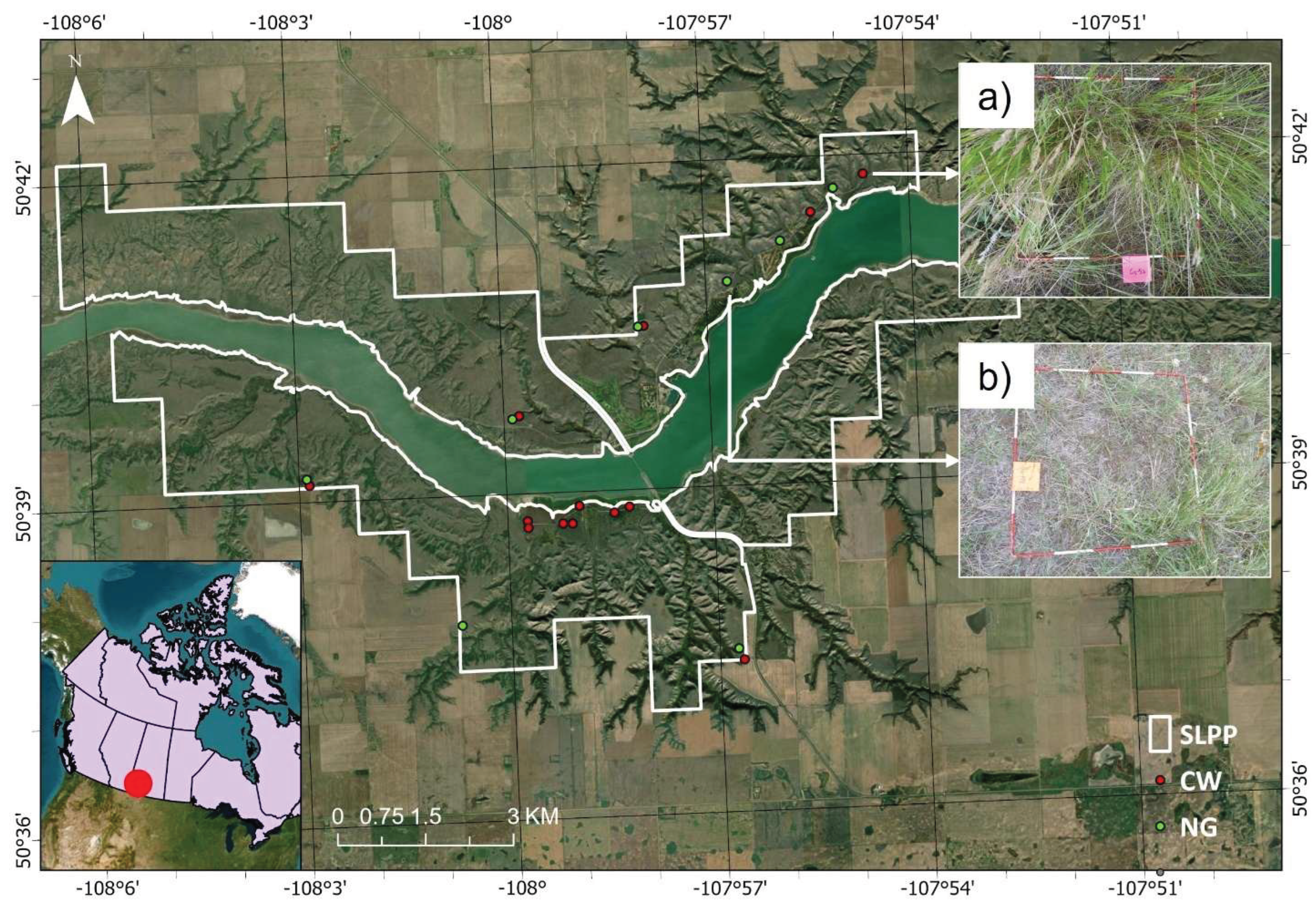
Figure 2.
Plot design for data collection over 20 m by 20 m sites in Saskatchewan Landing Provincial Park (SLPP). N, E, W, and S indicate the North, East, West, and South cardinal directions, respectively.
Figure 2.
Plot design for data collection over 20 m by 20 m sites in Saskatchewan Landing Provincial Park (SLPP). N, E, W, and S indicate the North, East, West, and South cardinal directions, respectively.
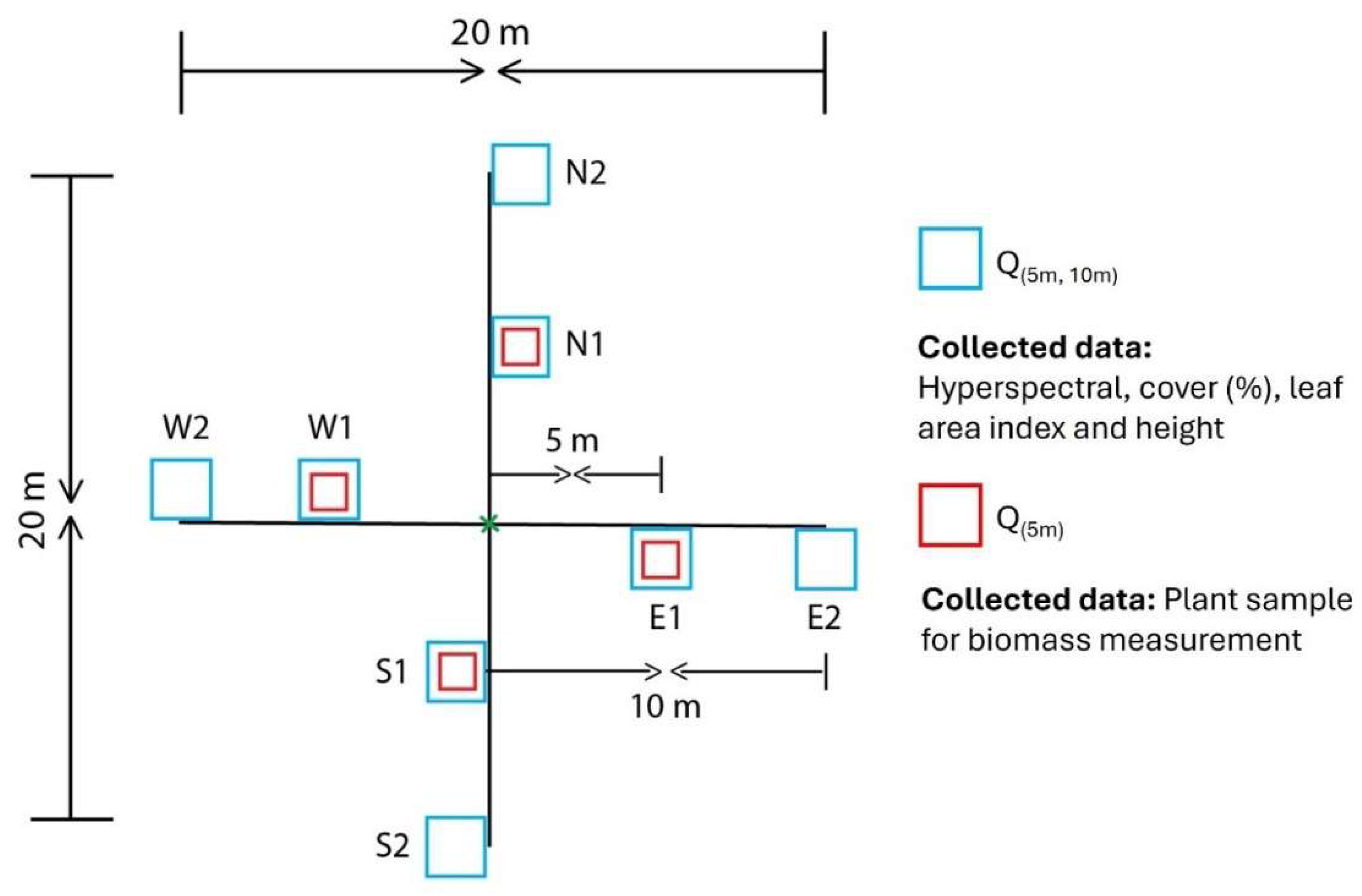
Figure 4.
Mean spectral profile of Crested Wheatgrass and Native grass collected by field spectroradiometer. Blue shaded regions indicate significant differences (p<0.05) between Crested Wheatgrass and native grass reflectance.
Figure 4.
Mean spectral profile of Crested Wheatgrass and Native grass collected by field spectroradiometer. Blue shaded regions indicate significant differences (p<0.05) between Crested Wheatgrass and native grass reflectance.
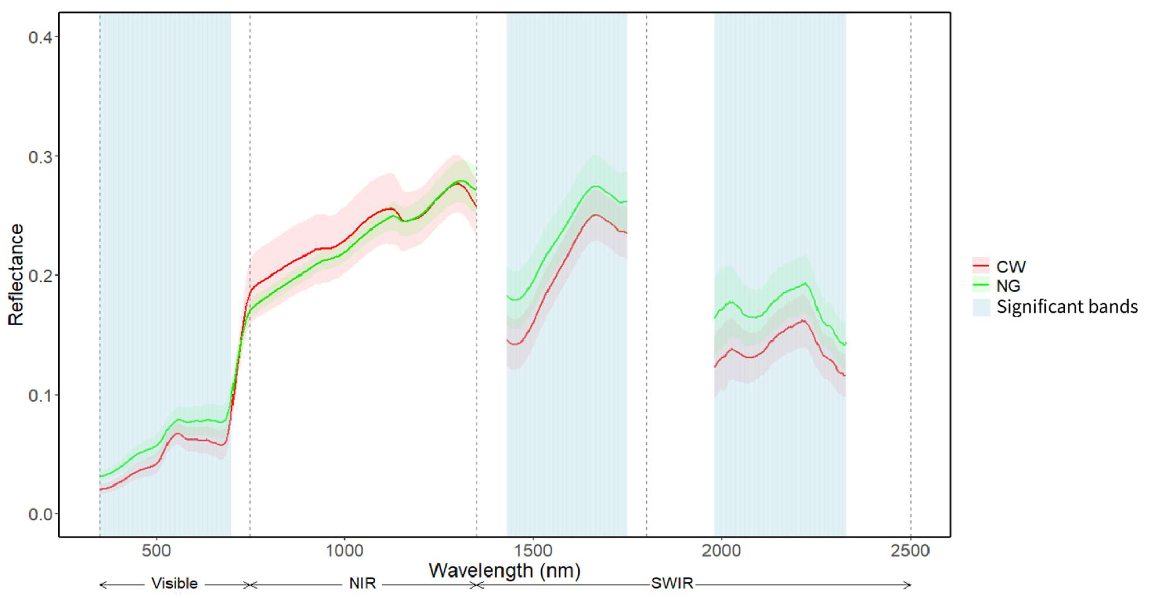
Figure 5.
Simulated PlanetScope SuperDove spectral data. Blue shaded regions indicate significant differences (p < 0.05) between Crested Wheatgrass and native grass reflectance (Larger font size).
Figure 5.
Simulated PlanetScope SuperDove spectral data. Blue shaded regions indicate significant differences (p < 0.05) between Crested Wheatgrass and native grass reflectance (Larger font size).
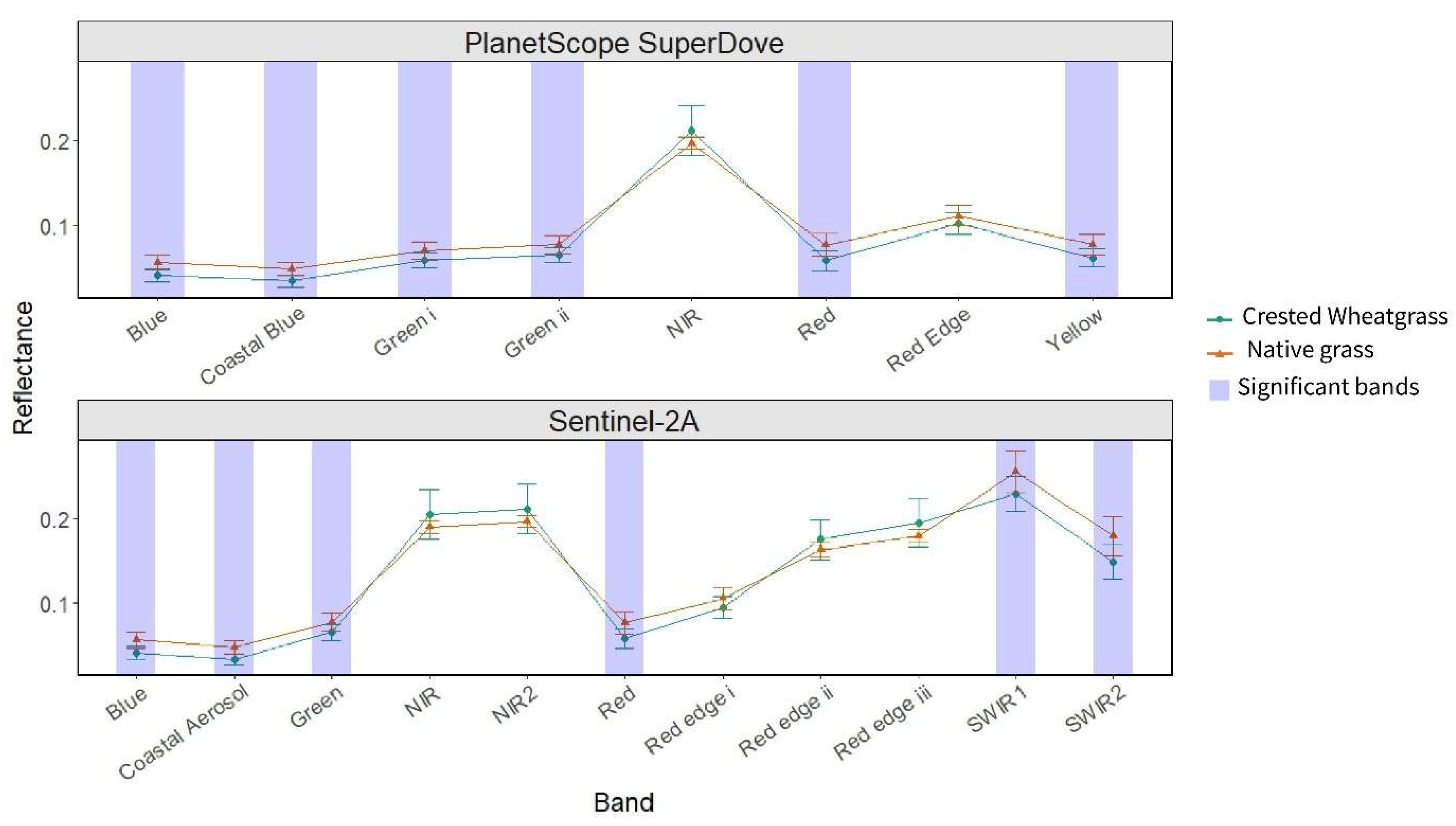
Figure 6.
Result of Linear regression models with interaction showing the slope difference between the relationship of hyperspectral indices and biophysical properties. pint < 0.05 indicates a significant difference between the slopes of Crested Wheatgrass and native grass.
Figure 6.
Result of Linear regression models with interaction showing the slope difference between the relationship of hyperspectral indices and biophysical properties. pint < 0.05 indicates a significant difference between the slopes of Crested Wheatgrass and native grass.
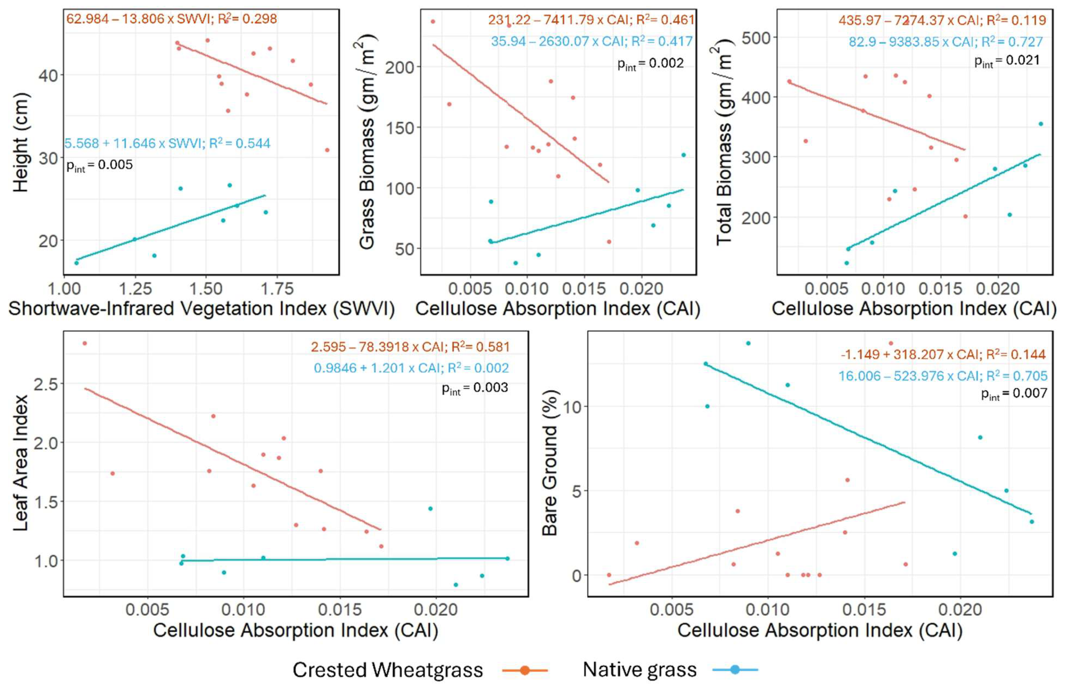
Figure 7.
Result of Linear regression models with interaction showing the slope difference between the relationship of simulated PlanetScope SuperDove spectral indices and biophysical properties. pint < 0.05 indicate a significant difference between the slopes of Crested Wheatgrass and native grass.
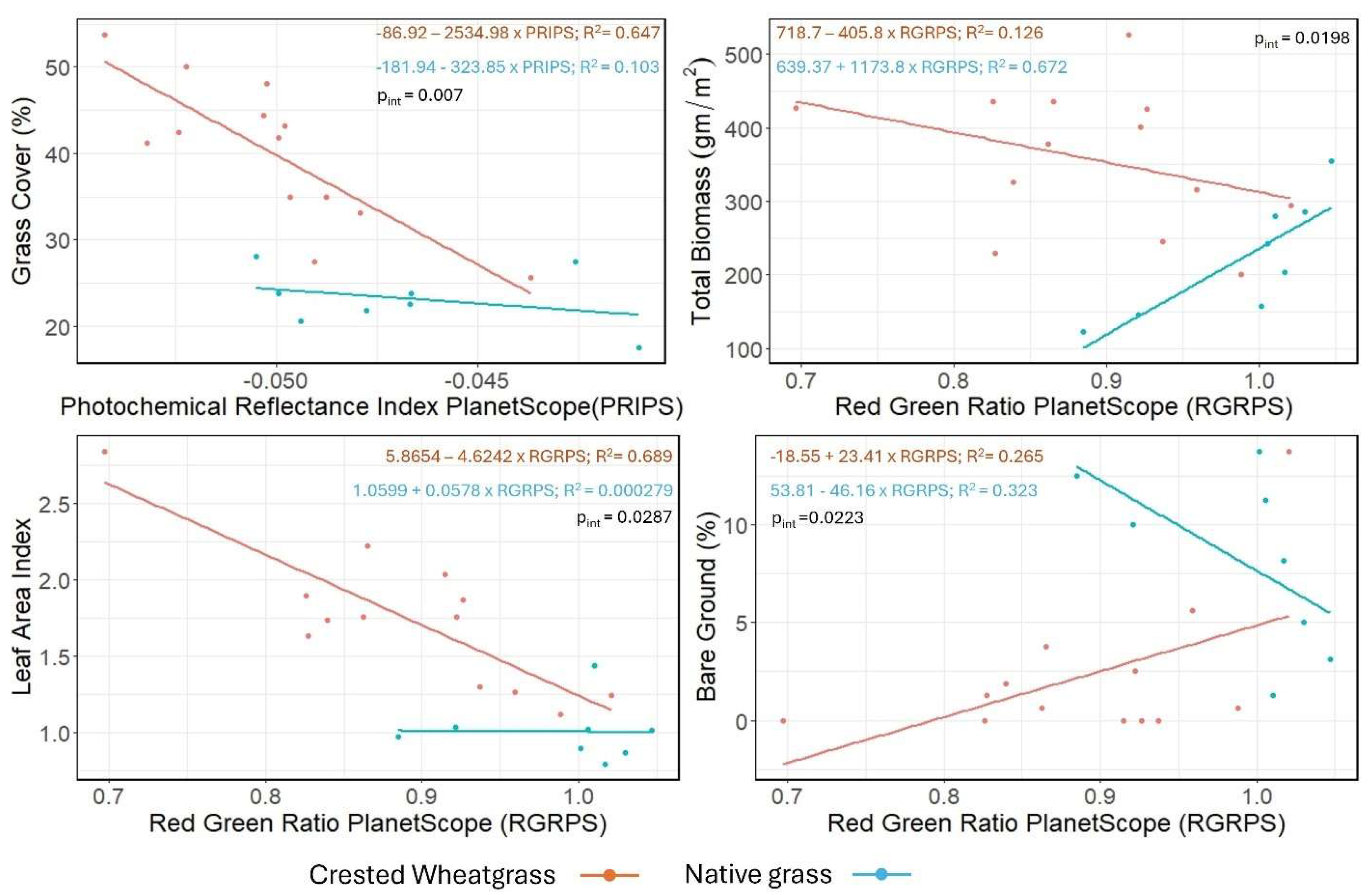
Figure 8.
Result of Linear regression model with interaction showing the slope difference between the relationship of simulated Sentinel-2A spectral indices and biophysical properties. pint < 0.05 indicate a significant difference between the slopes of Crested Wheatgrass and native grass.
Figure 8.
Result of Linear regression model with interaction showing the slope difference between the relationship of simulated Sentinel-2A spectral indices and biophysical properties. pint < 0.05 indicate a significant difference between the slopes of Crested Wheatgrass and native grass.
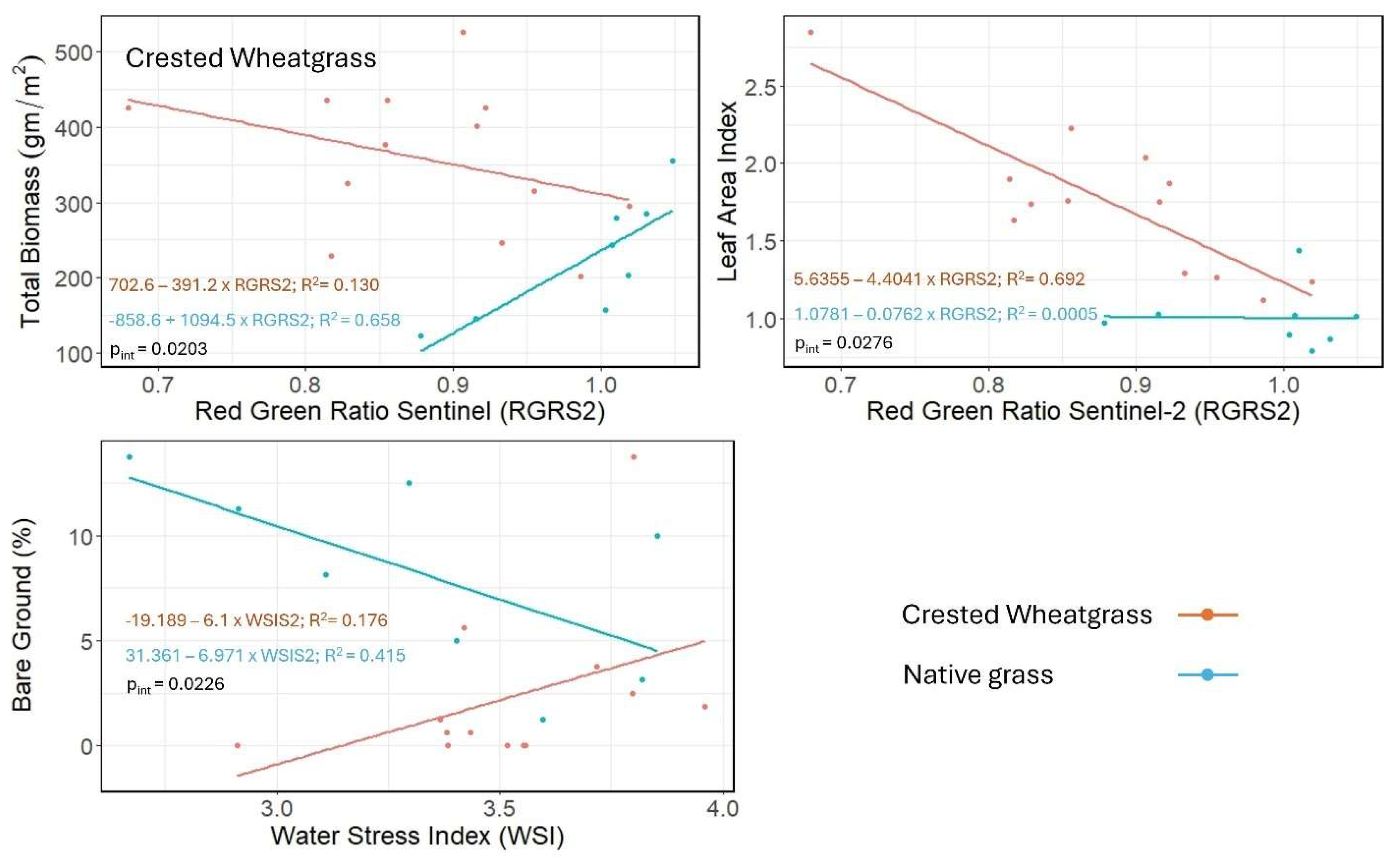

Table 1.
List of Hyperspectral indices used in this study. In this table, “R” represents reflectance and preceding numbers following R indicate wavelengths in nm.
Table 1.
List of Hyperspectral indices used in this study. In this table, “R” represents reflectance and preceding numbers following R indicate wavelengths in nm.
| Properties | Hyperspectral indices | Equation | Citation | Sentinel-2A equivalent | PlanetScope SuperDove equivalent |
| Pigment |
Normalized Differenced Vegetation indices (682-553) | (R682 – R553) / (R682 + R553) | [43] | (RB4 – RB3) / (RB4 + RB3) | (RB6 – RB4) / (RB6 + RB4) |
| Carotenoid Reflectance Index I (CRI 1) | (1/R510) - (1/R550) | [44,45] | (1/RB2) - (1/RB3) | (1/RB2) - (1/RB3) | |
| Red Green Ratio (RGR) | [45,46] | RB4/RB3 | RB6/RB4 | ||
| Photochemical reflectance index (PRI) | (R531 – R570) / (R531 + R570) | [46] | NA | (RB3 – RB4)/ (RB3 + RB4) | |
| Anthocyanin Reflectance Index I (ARI 1) | (1/R550) - (1/R700) | [47] | NA | NA | |
| Simple Ratio (SR) | R700 / R670 | [45,48] | NA | NA | |
| Modified Chlorophyll Absorption Ratio Index 2 (MCARI2) | ((R 700 - R 670) - 0.2 * (R 700 - R 550)) * (R 700 - R 670) | [49] | NA | NA | |
| Transformed Chlorophyll Absorption Reflectance Index (TCARI) | 3 * ((R700 - R670) - 0.2 * (R700 - R550)) * (R700 / R670) | [49] | NA | NA | |
| Simple ratio pigment index (SRPI) | R430/R680 | [50] | NA | NA | |
| Biochemical properties | Cellulose Absorption Index (CAI) | ((R2000 + R2200) / 2) – R2100 | [45,48] | RB12/RB11 | NA |
| Normalized Difference Nitrogen Index (NDNI) | (log (1/R1510) - log (1/R1680)) / (log (1/R1510) + log (1/R1680)) | [51] | NA | NA | |
| Stress indicator |
Yellowness Index (YI) | (R567– 587 – 2R616-636 + R656-676) / Δλ2 | [52,53] | NA | (RGreenII– 2RYellow + RRed) / Δλ2 |
| Disease- 2 (WSI) | R1660/R550 | [54] | RB11/RB3 | NA | |
| Structural properties |
Shortwave-Infrared Vegetation Index (SWVI) | 37.72 * (R2210 – R2090) + 26.27 * (R2280 – R2090) + 0.57 | [55] | NA | NA |
| Soil Adjusted Total Vegetation Index (SATVI) | ((R1650-R680)/(R1650+R680+L))(1+L) – R2215/2 | [56] | ((RB11 - RB4) / (RB11 + RB4+ L)) * (1 + L) - (RB12 / 2) | NA | |
| Hyperspectral biomass and structural index | NA | [57] | (RB11 - RB4) / (RB11 + RB4) | NA |
Table 2.
Descriptive statistics of biophysical properties of Crested Wheatgrass and native grass.
| Biophysical properties | Mean (Std) | Coefficient of variation | |||
|---|---|---|---|---|---|
| Crested Wheatgrass | Native grass | p | Crested Wheatgrass | Native grass | |
| Grass cover (%) | 40 (8.4) | 23 (3.5) | <0.001 | 0.21 | 0.15 |
| Standing dead cover (%) | 11 (5.3) | 9 (4.5) | Not significant | 0.48 | 0.49 |
| Litter cover (%) | 45 (8.4) | 48 (9.1) | Not significant | 0.19 | 0.19 |
| Bare ground (%) | 2 (3.8) | 8 (4.6) | <0.01 | 0.167 | 0.56 |
| Shrub cover (%) | 1 (1.9) | 2.5 (2.7) | Not significant | 0.201 | 0.108 |
| Height (cm) | 40.5 (4.1) | 22.3 (3.5) | <0.001 | 0.10 | 0.16 |
| Leaf area index | 1.7 (0.5) | 1.0 (0.19) | <0.001 | 0.27 | 0.19 |
| Grass biomass (gm/m2) | 150.7 (50.0) | 75.5 (29.8) | <0.01 | 0.33 | 0.39 |
| Total Biomass (gm/m2) | 356.9 (96.7) | 224.0 (80.6) | <0.01 | 0.27 | 0.35 |
| Dead biomass (gm/m2) | 194.5 (67.4) | 130.6 (60.4) | <0.05 | 0.35 | 0.46 |
| Shrub biomass (gm/m2) | 10.6 (17.4) | 7.0 (9.0) | Not significant | 0.165 | 0.128 |
Table 3.
Results of the significant Linear regression models with interaction showing the slope difference (pint), variance explained by the model (R2), and equation for the linear model between Spectral indices (Hyperspectral, PlanetScope SuperDove and Sentinel-2A) and biophysical properties. Here the Crested Wheatgrass is the base level (for Crested Wheatgrass, Species = 0 and for native grass, native grass = 1) and SWVI, CAI, RGRPS, RGRS2, WSI and PRIPS indicates Short wave vegetation index, Cellulose absorption index, Red green ratio PlanetScope SuperDove, Red green ratio Sentinel-2A, Water stress index and Photochemical reflectance index PlanetScope SuperDove respectively.
| Biophysical properties (Dataset type) | Equation (β0 + β1 x Spectral indices + β2 x Species + β3 x (Spectral indices x Species)) |
R2 | pint |
|---|---|---|---|
| Height (Hyperspectral) | 62.984 − 13.806 × SWVI − 57.416 × Species + 25.452 × (SWVI × Species) | 0.904 | 0.005 |
| Grass biomass (Hyperspectral) | 231.22 − 7411.79 × CAI − 195.28 × Species + 10041.86 × (CAI × Species) | 0.6919 | 0.002 |
| Total biomass (Hyperspectral) | 435.97 − 7274.37 × CAI − 353.07 × Species + 16658.22 × (CAI × Species) | 0.5458 | 0.02 |
| Total biomass (PlanetScope SuperDove) | 718.7 - 405.8 × RGRPS -79.33 × Species + 1579.6 × (RGRPS × Species) | 0.5389 | 0.019 |
| Total biomass (Sentinel-2A) | 702.6 -391.2 × RGRS2 -1561.2 × Species + 1485.7 × (RGRS2 × Species) |
0.538 | 0.02 |
| Leaf area index (Hyperspectral) | 2.5956 − 78.3918 × CAI − 1.6110 × Species + 79.5931× (CAI × Species) | 0.7558 | 0.003 |
| Leaf area index (PlanetScope SuperDove) | 5.8654 -4.6242 × RGRPS -4.8055 × Species + 4.5664 × (RGRPS × Species) |
0.8066 | 0.028 |
| Leaf Area Index (Sentinel-2A) | 5.6355 -4.4041 × RGRS2 -4.5574 × Species + 4.3279 × (RGRS2 × Species) |
0.8081 | 0.027 |
| Bare ground cover (Hyperspectral) | −1.149 + 318.207 × CAI + 17.155 × Species − 842.183 × (CAI × Species) | 0.6027 | 0.007 |
| Bare Ground (PlanetScope SuperDove) | -18.55 + 23.41× RGRPS +72.36 × Species -69.57× (RGRPS × Species) | 0.533 | 0.022 |
| Bare ground cover (Sentinel-2A) | -19.189 + 6.101× WSI + 50.550 × Species - 13.072× (WSI × Species) | 0.5281 | 0.022 |
| Grass Cover (PlanetScope SuperDove) | -86.95− 2534.98 × PRIPS − 94.99 × Species + 2211.13 × (PRIPS × Species) | 0.8394 | 0.007 |
Disclaimer/Publisher’s Note: The statements, opinions and data contained in all publications are solely those of the individual author(s) and contributor(s) and not of MDPI and/or the editor(s). MDPI and/or the editor(s) disclaim responsibility for any injury to people or property resulting from any ideas, methods, instructions or products referred to in the content. |
© 2025 by the authors. Licensee MDPI, Basel, Switzerland. This article is an open access article distributed under the terms and conditions of the Creative Commons Attribution (CC BY) license (http://creativecommons.org/licenses/by/4.0/).
Copyright: This open access article is published under a Creative Commons CC BY 4.0 license, which permit the free download, distribution, and reuse, provided that the author and preprint are cited in any reuse.


