Submitted:
27 August 2025
Posted:
28 August 2025
You are already at the latest version
Abstract
Inland lakes across the United States are increasingly impacted by nutrient pollution, sedimentation, and algal blooms, with significant ecological and economic consequences. While satellite-based monitoring has advanced our ability to assess water quality at scale, many lakes remain analytically underserved due to their spatial heterogeneity and the multivariate nature of pollution dynamics. This study presents an integrated framework for detecting spatiotemporal pollution patterns using satellite remote sensing, trend segmentation, hierarchical clustering and dimensionality reduction. Taking Horseshoe Lake (Illinois) as a case study, we analyzed Sentinel-2 imagery from 2020–2024 to derive chlorophyll-a (NDCI), turbidity (NDTI), and total phosphorus (TP) across five hydrologically distinct zones. Breakpoint detection and modified Mann-Kendall tests revealed both abrupt and seasonal trend shifts, while correlation and hierarchical clustering uncovered inter-zone relationships. To identify lake-wide pollution windows, we applied Kernel PCA to generate a composite pollution index, aligned with the count of increasing trend segments. Two peak pollution periods, late 2022 and late 2023, were identified, with Regions 1 and 5 consistently showing high values across all indicators. Spatial maps linked these hotspots to urban runoff and legacy impacts. The framework captures both acute and chronic stress zones and enables targeted, seasonal diagnostics. The approach demonstrates a scalable and transferable method for pollution monitoring in morphologically complex lakes and supports more targeted, region-specific water management strategies.
Keywords:
inland lake water quality
; remote sensing
; spatiotemporal analysis
; ecological stress mapping
; kernel PCA
1. Introduction
In the U.S., there are over 123,000 lakes larger than 4 ha, plus countless smaller ones that dominate in number and collectively span approximately 9.5 million hectares [1]. These water bodies serve as ecological hotspots, providing critical services such as flood retention, recreation, and biodiversity support, while also boosting local economies and community well-being [1,2]. However, many of these lakes are increasingly threatened by nutrient pollution, sedimentation, and harmful algal blooms, often resulting from upstream land-use practices and legacy contaminants [3,4]. Water pollution, particularly nutrient-driven degradation, is estimated to cost the U.S. economy over $4.3 billion annually in water treatment, property devaluation, and lost recreational use [5]. Most inland lakes often remain under-monitored due to their spatial complexity, seasonal variability, and the high cost of maintaining traditional in-situ water quality networks [2,4]. These challenges highlight the growing need for scalable, cost-effective data collection methods and processing techniques to support proactive lake management in a changing climate [6,7].
Satellite remote sensing has significantly enhanced our ability to monitor the health of inland lakes [8,9]. Multispectral satellite missions such as Sentinel-2 and Landsat-8/9 allow for the extraction of key water quality indicators at high spatial and temporal resolutions [10,11,12]. The emergence of cloud-based platforms, such as Google Earth Engine (GEE) [13], NASA’s AppEEARS [14], and OpenET [15], has further expanded the accessibility, processing efficiency, and analytical potential of satellite-derived data. In recent years, researchers have increasingly combined these technologies to assess and visualize lake water quality across space and time. For example, Landsat imagery has been used for chlorophyll and organic matter retrieval [16,17,18], while Sentinel imagery has been applied to assess spatial and temporal trends in chlorophyll-a [19,20,21]. These studies have laid valuable groundwork for satellite-based lake monitoring. However, relying on a single parameter can limit our understanding of the multiple, interacting factors that contribute to water quality degradation. This is particularly true for urban inland lakes, where water conditions are shaped by a complex mix of industrial discharge, stormwater runoff, and nutrient inputs from surrounding land uses [22,23].
In response, recent research has begun to incorporate multiple indicators such as turbidity and total phosphorus to provide a more complete picture of lake health [24,25,26]. This multi-parameter approach allows for a more realistic assessment of pollution dynamics in complex lake environments [27]. However, many studies still rely on basic trend detection methods like linear regression or the Mann–Kendall test, which assume gradual changes over time [28,29,30]. As a result, they may overlook sudden pollution spikes, regime shifts, or seasonal disruptions that are critical for early warning and targeted management [31,32]. Moreover, not accounting for temporal autocorrelation can lead to misinterpretation of trend strength or significance [32]. These gaps highlight the need for more refined methods that can detect abrupt changes and capture both short-term variability and long-term patterns in water quality.
Many inland lakes, especially larger or oxbow types, are not spatially uniform. Natural landforms, engineered barriers, or variable inflow sources often divide them into distinct sub-basins. These divisions lead to localized regimes shaped by different levels of industrial discharge, stormwater runoff, agricultural input, and sedimentation. Treating such systems as homogeneous can obscure important spatial patterns and mislead intervention strategies [33,34]. In these cases, traditional time-series analyses with multiple water quality parameters may also fall short. There is a growing need to complement them with spatially-aware approaches that account for intra-lake heterogeneity and detect zone-specific trends [35,36]. To better capture these internal dynamics, researchers have applied techniques such as pixel-based trend analysis [37,38], zonal averaging [39,40], moving window statistics [41,42], and region-specific comparisons [43,44]. While useful, these methods often rely on predefined spatial units and may miss shared or emergent pollution dynamics across regions [45,46,47,48]. This challenge becomes more complex when multiple water quality parameters are tracked together over long periods [6]. For effective lake management and policy planning, it is essential to move beyond isolated parameter analysis and instead synthesize multivariate time series into an integrated framework that reflects overall ecological stress. To address this, researchers have used techniques such as Self-Organizing Maps (SOMs) [49,50], Multivariate Autoregressive Models (MARs) [51,52], and index-based aggregations [53,54]. However, these methods often fall short in detecting synchronized change events across parameters and space, or in identifying the most critical time windows for intervention [55,56]. This creates a methodological gap, particularly for spatially heterogeneous lakes, that calls for more integrative and spatially dynamic approaches to pollution monitoring and decision-making.
In the current study, we address these methodological and monitoring challenges by developing an integrated framework for long-term water quality assessment in spatially heterogeneous lakes. To capture localized pollution, we divide the lake into physically distinct zones and analyze region-specific time series of chlorophyll (NDCI), turbidity (NDTI), and total phosphorus (TP). To overcome the limitations of basic trend methods, we apply breakpoint detection and modified Mann–Kendall tests that can capture both gradual changes and abrupt shifts. To better understand inter-zone relationships and ecological synchronization, we use correlation analysis and hierarchical clustering to detect temporal alignment and spatial similarity. Finally, to move beyond isolated trends and identify lake-wide pollution events, we employ Kernel PCA to reduce multivariate time series into a composite pollution index, which is overlaid with trend counts to pinpoint critical periods of ecological stress. Using Horseshoe Lake in Madison County, Illinois as a case study, this framework demonstrates a scalable and transferable approach that combines satellite remote sensing, zone-wise analytics, and advanced statistical tools to support pollution detection.
2. Materials and Methods
2.1. Study Area
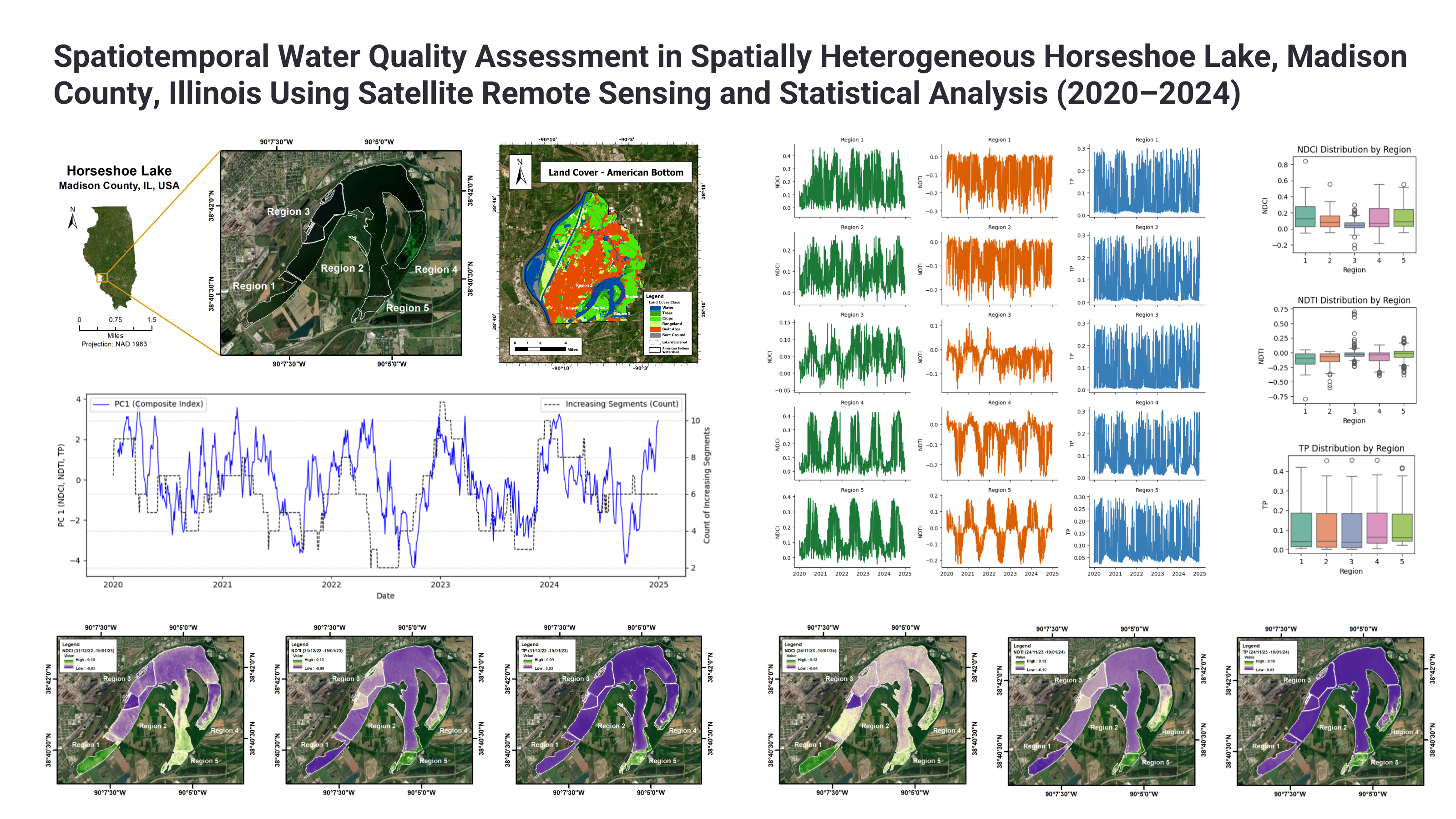
Horseshoe Lake is a shallow oxbow lake (~2 meters average depth) located in the Mississippi River floodplain in Granite City, Madison County, Illinois, approximately 2 miles east of the river and 4 miles from St. Louis. The lake spans ~2,100 acres, including Walkers Island, and plays a vital role in flood retention, recreation, and wildlife habitat. As presented in Figure 1, the lake is physically divided into five distinct regions by visible natural and constructed separations, allowing for regional differentiation in water quality conditions. Stormwater runoff from Granite City enters the lake through three culverts: one at the north end (from Nameoki Ditch), two at the northeast end (from Elm Slough and Long Lake), and nine culverts at the east end (discharging agricultural runoff). In addition, Granite City Steel historically drew intake water from the Mississippi River and discharged up to 25 million gallons per day (mgd) of treated effluent into the lake’s west side [57,58]. Occasional flood water diversions also arrive from the Cahokia Drainage Canal, and runoff from surrounding areas contributes further.
2.2. Data and Tools Used
2.2.1. Data Used
In this study, we used the Sentinel-2 Surface Reflectance Harmonized (S2_SR_HARMONIZED) dataset available on Google Earth Engine, covering the period from January 2020 to December 2024 [59]. The dataset is part of the Copernicus Program operated by the European Space Agency and, as shown in Table 1, provides multispectral imagery with spatial resolutions ranging from 10 to 60 meters. With a revisit frequency of approximately five days, it enables consistent monitoring of surface water bodies. The imagery includes atmospherically corrected surface reflectance values, making it well-suited for water quality assessments over time.
2.2.2. ArcGIS Pro
Esri ArcGIS Pro 3.2 is a widely used desktop GIS software for spatial analysis and mapping [60]. In this study, it was used to develop and manage the spatial framework. Horseshoe Lake was divided into eight physically distinct zones, based on separations observed in high-resolution basemaps and satellite imagery. ArcGIS Pro facilitated the creation of reference maps and the assignment of spatial attributes to satellite-derived water quality data. It also supported the export of zone-level shapefiles for use in water quality assessment within Google Earth Engine and statistical analysis in Google Colab. Overall, the platform enabled essential spatial operations and streamlined the geospatial workflow.
2.2.3. Google Earth Engine (GEE)
Google Earth Engine (GEE) is a cloud-based geospatial platform used in this study for satellite image retrieval, processing, and time-series compositing [13]. GEE allowed efficient access to multi-temporal, multi-spectral satellite datasets. Sentinel-2 satellite data from 2020 to 2024 was fetched for the analysis. Cloud masking was performed using the QA60 bitmask approach, which excludes pixels affected by clouds and cirrus contamination to improve the accuracy of water quality parameter estimation [62,63]. Using GEE’s JavaScript interface, indices such as NDVI, NDTI, and TP were computed across the predefined lake zones. The platform significantly reduced preprocessing time and eliminated the need for local storage, streamlining the analysis.
2.2.4. Programming Interface
This study used Google Colab, a free cloud-based Python development environment, to conduct time-series analysis, principal component analysis (PCA), correlation analysis, and hierarchical clustering [64]. Python (v3.10) and widely used libraries, including Pandas (v1.5.3) [65], NumPy (v1.22.4) [66], SciPy (v1.10.1) [67], Scikit-learn (v1.2.2) [68], Matplotlib (v3.7.1) [69], and Seaborn (v0.12.2) [70], were employed to perform breakpoint detection, trend estimation, and statistical pattern recognition. This programming workflow ensured reproducible and scalable analysis and enabled seamless integration with spatial datasets from ArcGIS Pro [60] and Google Earth Engine [61].
2.3. Methodology
This study used Sentinel-2 MSI satellite imagery from 2020 to 2024 to analyze long-term spatiotemporal patterns in water quality across Horseshoe Lake. The methodology flow diagram is presented in Figure 2. Cloud-contaminated pixels were removed using the QA60 bitmask approach, ensuring clean and consistent observations. This method is widely used in remote sensing and is particularly effective for studies requiring high temporal reliability and data accuracy [61,62,71]. The resulting multitemporal image collection was used to derive key water quality indices. Three satellite-derived indicators, NDCI, NDTI, and TP, were calculated and organized into time series for each of the lake’s predefined zones [72,73,74]. These time series were used in multiple analytical steps. First, breakpoint detection was performed using the Dynamic Programming (Dynp) algorithm to identify significant changes in water quality trends [76,77]. Each segmented trend was analyzed using the Mann–Kendall test with Yue–Wang modification to classify it as increasing, decreasing, or non-significant [78,79]. These trends were then aggregated and analyzed seasonally, annually, and monthly. Second, correlation analysis was conducted on both raw time series and trend summaries to examine temporal synchronization and variability among regions. These results supported the identification of inter-index relationships and seasonal patterns. Third, hierarchical clustering was applied to group zones with similar water quality profiles, allowing for spatial classification based on pollutant behavior [80]. In parallel, PCA and trend count analysis were employed to reduce dimensionality and identify key timestamps representing high pollution periods [81]. These timestamps were used to generate representative water quality maps. Together, these integrated analyses provided a detailed understanding of water quality dynamics, pollution intensity peaks, and spatial clustering, offering valuable insights for long-term lake monitoring and management.
2.3.1. Water Quality Indices
To assess lake water quality using satellite imagery, we selected three indicators that are commonly applied in aquatic remote sensing, namely the NDCI, NDTI, and TP. These indices help quantify biological productivity, turbidity, and nutrient enrichment, respectively.
- NDCI (Equation 1) estimates chlorophyll-a concentration and detects algal blooms by combining Sentinel-2 Band 5 (red-edge, B5) and Band 4 (red, B4). Areas with high values indicate elevated phytoplankton activity [72].NDCI = (B5 – B4)/(B5 + B4)
- NDTI (Equation 2) measures turbidity and suspended sediment levels using Sentinel-2 Band 4 (red, B4) and Band 3 (green, B3). Higher NDTI values typically correspond to poor water clarity due to sediment load [73].NDTI = (B4 – B3)/(B4 + B3)
2.3.2. Break Point and Trend Analysis
In all five regions of Horseshoe Lake, we conducted breakpoint and trend analysis using NDCI, NDTI, and TP observations from 2020 to 2024. The goal was to examine how water quality changed over time. We used the Dynp algorithm from the ruptures library to detect breakpoints [76,77]. These breakpoints mark points where significant changes occurred in the time series and are useful for identifying multiple shifts in long and noisy datasets. Each segment between the breakpoints was then analyzed using the Mann-Kendall test with the Yue–Wang modification [78], further supported by the pyMannKendall package [79]. This version of the test corrects for autocorrelation, which helps improve the accuracy of trend detection in environmental data. Trends were categorized as increasing, decreasing, or non-significant. We calculated how long each trend type lasted in days and grouped these durations by year, season, and month. Finally, we converted the results into percentages and used bar plots to show seasonal and long-term patterns in water quality across the lake.
2.3.3. Time Series & Trends Correlations
To assess how water quality patterns vary across Horseshoe Lake, we conducted correlation analysis using both raw time-series data and long-term trends. Regional time series for key parameters (NDCI, NDTI, TP) were arranged into pivot tables, and Pearson correlation coefficients were used to measure similarity in temporal patterns between zones [82,83]. For trend analysis, we used pre-labeled directional trends (increasing, decreasing, or non-significant) from earlier time-series analyses. These trends were converted into numeric values (+1, −1, 0) and averaged by year to allow comparison across regions [84]. We then created correlation matrices to explore how consistent or different the trends were across zones. Heatmaps helped visualize these relationships, offering insight into both short-term patterns and long-term changes in water quality.
2.3.4. Hierarchical Clustering for Regional Grouping
To identify which zones of Horseshoe Lake are more or less affected by water quality issues, we applied hierarchical clustering using NDCI, NDTI, and TP time series as input features. For each zone, the median value of these parameters was calculated to represent overall conditions during the study period. The median was chosen over the mean to reduce the influence of short-term fluctuations and outliers. Before clustering, all values were standardized using z-score normalization to ensure that each parameter contributed equally to the analysis [85]. We used Ward’s linkage method, which forms clusters by minimizing the variance within each group [86]. This method was selected because it tends to produce compact, well-separated clusters, making it particularly suitable for identifying distinct patterns in environmental data across lake zones. A dendrogram was created to visualize how regions group together based on their water quality profiles. We used the Silhouette score [87] and Davies–Bouldin score [88] to evaluate the separation between clusters. The Silhouette score measures how similar each region is to its own cluster compared to others, with higher values indicating better-defined groups. The Davies–Bouldin score reflects intra-cluster compactness and inter-cluster separation, where lower values suggest more distinct and tighter clusters.
2.3.5. PCA & Trend Count Analysis for Maximum Pollution Windows
To identify the period of maximum pollution across all lake zones, we conducted a composite analysis that combined PCA with the count of increasing trend segments. Region-wise time series data were first reshaped into a consistent format containing 15 variables (three indicators across five regions). We used Kernel PCA (K-PCA) to reduce the dataset’s dimensionality and extract a single composite index (PC1) that reflects overall pollution levels [89]. K-PCA is a powerful technique for reducing dimensionality while capturing complex, nonlinear relationships in multivariate data [90]. The key parameters used in K-PCA included the kernel type, set to rbf, the number of components (n_components = 3), gamma (γ = 0.1) to control the curvature of the mapping, and coef0 = 10 to adjust the offset in the kernel function. These settings enabled effective dimensionality reduction while preserving nonlinear patterns across the 15 water quality time series. We then plotted PC1 over time and overlaid it with the number of regions simultaneously showing increasing trends. The periods where high PC1 values coincided with peak counts of increasing segments were identified as the lake’s maximum pollution periods. This integrated method allowed us to capture both the intensity and timing of water quality degradation with improved clarity.
2.3.6. Spatial Mapping for High-Pollution Windows
To assess spatial pollution patterns during the two high-pollution windows, we used ArcGIS Pro (version 3.2) [60] to calculate and map the average values of NDCI, NDTI, and TP across the five regions of Horseshoe Lake. Satellite images corresponding to the selected high-pollution periods were downloaded, and the Cell Statistics tool with the mean function was applied to compute the average of all satellite images for each pollution window. The results were then visualized as spatial distribution maps for each parameter and time window, highlighting spatial variability in pollution intensity.
3. Results
3.1. Time Series Extraction of Water Quality Indicators
Horseshoe Lake, a shallow inland water body surrounded by agricultural land and urban development, is particularly vulnerable to nutrient-rich runoff, sediment loading, and algal proliferation. These processes contribute to episodic increases in chlorophyll-a, turbidity, and phosphorus, key indicators of eutrophication and declining water quality. To evaluate these dynamics, the current study utilized NDCI, NDTI, and TP indices. A five-year stack of Sentinel-2 MSI imagery (2020–2024) was processed in Google Earth Engine. Cloud-contaminated pixels were masked using the QA60 bitmask, and image data were spatially extracted for each of the lake’s five zones. For each zone, we computed mean index values per image, generating time series with a nominal 5-day revisit interval. Figure 3 presents the time series of NDCI, NDTI, and TP across all zones. These subplots reveal distinct seasonal patterns and inter-annual variability in water quality. Notably, certain regions exhibit consistently higher turbidity (region 5) or chlorophyll (region1) concentrations, reflecting localized sources of disturbance or stagnation. The QA60 masking was validated through visual inspection and temporal stability checks during known cloudy periods, ensuring reliable time series inputs for subsequent analyses. To assess the distribution and variability of water quality conditions, we generated box-and-whisker plots (Figure 4) for NDCI, NDTI, and TP across the five lake zones. Region 1 had the highest NDCI median (0.083) and upper quartile (Q3) value (0.2065), indicating elevated chlorophyll concentrations, while Region 5 recorded the lowest median (0.0305). NDTI medians followed a similar trend, with Region 1 at –0.0510 and Region 5 close to zero (–0.0025), suggesting clearer water in the lake’s peripheral zones. TP values peaked in Region 5, with a median of 0.1875 and a maximum of 0.412, while Region 2 had the lowest median (0.0460). Overall, Regions 1 and 5 consistently showed higher pollution levels across all indicators, marking them as potential hotspots for eutrophication and turbidity.
3.2. Trends in Water Quality Parameters
Figure 5, Figure 6, and Figure 7 present a comprehensive assessment of water quality trends in Horseshoe Lake from 2020 to 2024 using NDCI, NDTI, and TP, respectively. Each figure includes two sets of subplots. The first set presents region-specific time series with breakpoints and trend segments classified as increasing, decreasing, or not significant. The second set summarizes trends at annual, seasonal, and monthly levels. These visualizations help explain the spatial (region-wise) and temporal changes in water quality.
- Trends in NDCI: The left part of Figure 5 shows NDCI trend segments across five lake regions. Region 1 experienced a fairly balanced sequence of increasing and decreasing trends, with a few non-significant periods. It shows recurring fluctuations, especially between 2021 and 2023. Region 2 started with short-term declines, followed by frequent alternating increases and decreases. Region 3 showed higher variability, with short trend segments and more frequent declines during 2021–2023. Region 4 had longer periods of consistent decline, especially from mid-2020 to late 2022, with limited signs of recovery. In contrast, Region 5 experienced some of the longest periods of both increase and decrease. It showed extended rises in NDCI during 2022 and early 2024, followed by a decline through the end of the study period. The right set of subplots summarizes trend distributions across annual, seasonal, and monthly scales for NDCI. Annually, decreasing trends dominated in 2020 and 2023, while 2021 and 2022 showed more frequent increases. Seasonally, fall had the strongest NDCI declines, with 86% of periods showing decreasing trends. Spring and summer displayed a mix of increases and decreases. Winter recorded the highest share of increasing trends at 58%. Monthly patterns followed these trends, with February and July showing peaks in increases, while September and October were entirely marked by declines.
- Trends in NDTI: The left side of Figure 6 shows NDTI trends from 2020 to 2024 across the five lake regions. Region 1 had a mix of trends, with several short periods of increase and a few longer decreasing segments, showing alternating turbidity behavior. Region 2 showed mostly increasing trends early on, but more decreasing periods appeared between 2021 and 2023. A few increases returned in 2024. Region 3 was the most dynamic, with many short segments and a balance of increases and decreases. However, there was a cluster of persistent increases from late 2022 through 2024. Region 4 was dominated by long periods of decreasing turbidity from 2021 to 2023, followed by several shorter increases, suggesting recovery followed by new disturbances. Region 5 had the most consistent increases, especially in 2020, late 2022, and throughout 2024. The right panel of Figure 6 shows NDTI trends by year, season, and month. In 2020 and 2023, increasing trends were most common, reaching up to 59%. In 2021 and 2024, decreasing trends were more frequent, reaching 55% to 58%. Spring had the highest share of decreasing trends at 74%. Fall showed the most increasing trends at 77%. Summer had a mix of both. Winter showed nearly equal shares of increases and decreases. At the monthly level, April and May had the strongest decreases, with up to 88%. August, October, and November showed the highest increases.
- Trends in TP: The left panel of Figure 7 shows TP trends in Horseshoe Lake from 2020 to 2024. Region 1 had mostly increasing trends throughout the period, with short declines in late 2020 and mid-2021. Region 2 showed a mix of patterns, with early increases, mid-period declines, and more increases in 2024. Region 3 started with mostly increasing and non-significant trends, but showed consistent declines in mid to late 2022 and again in 2024. Region 4 had an early increasing phase, followed by a long declining trend from mid-2021 to late 2023, then returned to short increases and stable periods. Region 5 showed the most prolonged and consistent increases, especially from early 2020 and again in late 2023 to the end of 2024, with only a few brief declining periods. The right of Figure 7 panel summarizes annual, seasonal, and monthly TP trends. In 2020, increasing trends were highest at 59%. In 2021 and 2022, decreasing trends were more common, peaking at 66% in 2022. Increases returned in 2023 and 2024. Summer had the highest share of decreasing trends at 64%. Fall showed the most increasing trends at 72%. Spring and winter had more balanced patterns. Monthly trends followed this pattern. June and September had the strongest decreases. October and November showed the highest increases, close to 100%. February and August had more non-significant trends.
Overall, the trends in NDCI, NDTI, and TP show both short-term variability and longer-term shifts in water quality across Horseshoe Lake. These patterns reflect seasonal cycles, spatial differences, and the need for continued monitoring to guide local management and restoration strategies.
3.3. Time Series & Trends Correlations
Figure 8 summarizes correlation matrices for both raw time series and trend-segmented values of NDCI, NDTI, and TP across the five lake regions. For the raw time series, NDCI and TP show consistently high correlations across most region pairs. In contrast, NDTI displays more varied and weaker associations. TP raw values exhibit strong alignment among all regions, with most correlation coefficients above 0.9. This reflects the lake-wide influence of nutrient-rich inflows and sediment resuspension that broadly affect phosphorus concentrations. NDCI raw values also show moderate to strong agreement, particularly between Region 2 and Regions 3 and 5. This suggests shared biological responses in adjacent zones influenced by common hydrological inputs. NDTI raw correlations drop substantially for Region 5 when compared with other zones. This is likely due to persistent turbidity stress from multiple agricultural culverts and shallow bathymetry that create localized sediment resuspension dynamics. For trend-based values, the correlation structure is more differentiated. NDCI trend correlations cluster more strongly among adjacent regions, such as Regions 2 and 3 or Regions 3 and 4. This shows that phytoplankton activity is synchronized in hydrologically connected zones. Isolated areas respond more independently. NDTI trend relationships are concentrated between Regions 2, 3, and 4. Correlations are near zero elsewhere. This pattern is consistent with shared stormwater inputs and sediment dynamics in the eastern and central portions of the lake. TP trend correlations remain moderate to high among Regions 1, 2, and 3. These areas receive steady nutrient inputs from urban and industrial inflows. Region 4 shows weaker alignment with others, reflecting its relative isolation and different inflow sources. Overall, these patterns indicate that while phosphorus and chlorophyll are influenced by lake-wide drivers, turbidity is more localized and spatially heterogeneous, tied closely to site-specific inflows and sediment conditions.
3.4. Hierarchical Clustering for Regional Grouping
As shown in Figure 9, hierarchical clustering grouped the five regions of Horseshoe Lake into three clusters based on their median values of NDCI, NDTI, and TP. The dendrogram illustrates similarity among regions, where lower linkage distances indicate stronger resemblance in water quality profiles. Regions 1 and 2 clustered together at a distance of 0.8, reflecting comparable conditions with moderate chlorophyll, low turbidity, and low phosphorus. Regions 4 and 5 merged at 1.3, both characterized by low chlorophyll but elevated turbidity and phosphorus. Region 3 joined the 1–2 cluster at 2.6, indicating intermediate conditions that partly overlap with the urban-influenced zones. The final division occurred at 4.2, separating the (1–2–3) group from the (4–5) group and highlighting a distinct nutrient–turbidity regime in the southeastern portion of the lake. Cluster validity indices (Silhouette = 0.26, Davies–Bouldin = 0.42) indicate moderate separation, suggesting that while clusters are distinguishable, inter-regional overlap persists due to shared but unevenly distributed pollution drivers.
3.5. PCA & Trend Count Analysis for Maximum Pollution Windows in HSL Lake
To identify a common window of maximum pollution across all lake regions, we first used Kernel PCA (K-PCA) to combine NDCI, NDTI and TP indicators across all the five regions into one composite index. As presented in Figure 10, the first principal component (PC1) captured about 80% of the total variance, making it a strong summary of overall water quality stress. We then counted the number of increasing trend segments across all regions to find when pollution was rising at multiple locations. Two time windows showed both high PC1 values and a high number of increases:
- 31 Dec 2022 – 15 Jan 2023: During this period, PC1 values stayed above 4.0, with a peak of 4.7. This shows strong pollution across chlorophyll, turbidity, and phosphorus. The number of increasing segments reached 11, the highest in the full time series. This suggests a fast and steady rise in pollution indicators.
- 24 Nov 2023 – 10 Jan 2024: In this window, PC1 values stayed high (between 3.5 and 4.1). The increasing trend count remained between 9 and 10. This shows a longer-lasting pollution event with steady upward changes in water quality indicators.
This result shows that combining PC1 with trend counts can detect both short pollution spikes and longer-lasting events. This method can improve how we monitor pollution over time and support early warning for harmful algal blooms in Horseshoe Lake.
3.6. Regional Water Quality Patterns During Pollution Peaks
Spatial distributions of NDCI, NDTI, and TP during the two identified pollution windows provide insights into how different regions of Horseshoe Lake responded to peak water quality stress. These patterns are illustrated in Figure 11 (for the first window: 31 Dec 2022 – 15 Jan 2023) and Figure 12 (for the second window: 24 Nov 2023 – 10 Jan 2024).
- 31 Dec 2022 – 15 Jan 2023: The NDCI map shows high chlorophyll levels in Region 1 and Region 5 (green areas), indicating strong algal activity. Region 2 has moderate values, mostly in its southern part. Region 3 records the lowest NDCI (purple), suggesting clearer water. Region 4 shows a mix of low and moderate values. These patterns suggest that biological stress was highest in the southern and southeastern zones, aligning with the PC1 pollution peak. The NDTI map highlights elevated turbidity in Region 5, likely from sediment or surface runoff. Region 4 has small patches of moderate turbidity. Regions 1, 2, and 3 mostly show low values (purple), reflecting clearer conditions. This suggests turbidity stress was concentrated in Region 5. TP values were also highest in Region 5 and parts of Region 4. These areas likely received nutrients from nearby agriculture or disturbed sediments. In contrast, Regions 1, 2, and 3 show low phosphorus levels. Together, these findings show that nutrient and turbidity-related pollution was localized in the southeastern part of the lake.
- 24 Nov 2023 – 10 Jan 2024: During this period, high NDCI values appear in Region 1 and parts of Region 5, indicating strong algal growth. Region 3 has the lowest chlorophyll levels, while Regions 2 and 4 show moderate values with a few high-value patches. The spatial spread points to increased biological stress in the southern and southeastern lake zones. Turbidity was again highest in Region 5, shown by green areas on the NDTI map. Region 4 has moderate turbidity, while the rest of the lake (Regions 1, 2, and 3) shows lower values. This indicates that physical disturbance was concentrated in Region 5. The TP map shows a similar pattern. Regions 4 and 5 had the highest phosphorus levels, suggesting nutrient inputs from runoff or sediments. The other regions remained low in TP. The overlap of high NDCI, NDTI, and TP confirms a strong, localized pollution hotspot in the southern zones during this window.
4. Discussion
The five-year analysis of Horseshoe Lake offers critical insight into the complex hydrological, ecological, and anthropogenic drivers shaping water quality variability in shallow floodplain lakes. By leveraging Sentinel-2 satellite data and advanced statistical techniques, this study captures both temporal dynamics and spatial heterogeneity in key water quality indicators. The following insights carry important implications for long-term monitoring, predictive modeling, and adaptive lake management strategies.
- Regional Drivers of Pollution and Spatial Heterogeneity: Horseshoe Lake is situated within the American Bottom watershed, a floodplain of the Mississippi River where land use is dominated by urban development and agriculture. The land cover distribution (Figure 13) provides critical context for interpreting spatial patterns in water quality. The consistently high chlorophyll levels in the north are best understood as a consequence of stormwater culverts draining Granite City into Region 1. This aligns with the elevated NDCI values and recurring increases in high chlorophyll concentration we observed, showing how concentrated urban inflows shape ecological conditions in that part of the lake. On the eastern margin, croplands surround Region 5 and deliver multiple agricultural discharges. This landscape setting helps explain why Region 5 emerged as the most persistent hotspot of turbidity and phosphorus enrichment. The combination of nutrient-rich inflows, shallow bathymetry, and sediment resuspension reinforces a chronic stress regime that was evident across multiple indicators and time windows. The western side of the lake has a different trajectory. Historically, industrial effluent from Granite City Steel (later Granite City Works) contributed a distinct loading source [57,58]. With operations now idled and discharges halted, this industrial signature has largely disappeared. As a result, Horseshoe Lake has become more strongly dependent on stormwater, agricultural runoff, and seasonal snowmelt as its external drivers of change. Inflows from Elm Slough, Long Lake, and the Cahokia Drainage Canal further reinforce the connectivity between watershed processes and lake dynamics, producing spatial synchrony among several central and eastern regions. Together, these patterns underscore the importance of considering both landscape context and hydrological connectivity in explaining water quality variation. The land cover map highlights how urban, agricultural, and historical industrial zones each leave distinct ecological fingerprints on different parts of the lake. This reinforces the need for region-specific management rather than a uniform intervention strategy.
- Temporal Disruption and Seasonality in Trends: Breakpoint detection revealed that water quality does not follow simple linear trajectories but is punctuated by abrupt changes. These shifts are often triggered by episodic storm events, flood diversions, or seasonal nutrient pulses. Seasonal trend summaries confirmed that fall and winter are periods of elevated risk, with frequent increases in turbidity and phosphorus even when algal activity is less visible. Such “latent stress” periods underscore the limitations of summer-centric monitoring campaigns and highlight the importance of year-round satellite-based assessments.
- Inter-Zonal Synchronization and Spatial Clustering: Correlation analysis and hierarchical clustering demonstrated that not all regions respond uniformly to external pressures. Regions 1 and 2 exhibited similar water quality behavior, reflecting shared exposure to urban runoff. Regions 4 and 5 consistently clustered together, reflecting common nutrient and turbidity stress from agricultural inflows and shallow bathymetry. Region 3 stood apart as a transitional zone, influenced by mixed inputs but buffered relative to the more polluted zones. These findings emphasize that lake-wide interventions may overlook critical spatial heterogeneity, and that tailored management strategies are required at the sub-regional scale.
- Implications for Monitoring and Adaptive Management: The integrated framework of this study, combining satellite remote sensing, statistical segmentation, clustering, and dimensionality reduction, provides a scalable model for monitoring complex inland lakes. The land cover map (Figure 13) strengthens this framework by spatially linking regional water quality dynamics with surrounding land-use drivers and inflow points. Importantly, the decline of industrial inputs from Granite City Works signals a new era in Horseshoe Lake’s hydrology, one where stormwater, agricultural runoff, and snowmelt dominate external loading. This transition reinforces the need for adaptive management strategies that prioritize watershed-scale interventions, control of nutrient-rich runoff, and enhanced resilience under climate-driven increases in extreme precipitation.
In sum, the integration of satellite observations, trend analytics, hierarchical clustering, and land cover mapping provides a robust and transferable framework for lake monitoring. This case study illustrates how openly available satellite data and cloud-based platforms such as Google Earth Engine [13] can generate high-resolution, management-relevant insights into pollutant dynamics and watershed–lake interactions. Beyond Horseshoe Lake, the approach can be scaled to other morphologically complex floodplain lakes, where evolving land-use patterns and shifting industrial activities alter the balance of external loading and ecological stress.
5. Conclusions
This five-year spatiotemporal assessment of Horseshoe Lake demonstrates the value of integrating satellite remote sensing with advanced statistical techniques to monitor inland lake water quality in morphologically complex systems. The analysis revealed persistent pollution hotspots in Regions 1 and 5, reflecting their unique exposure to external stressors. Region 1 is directly influenced by stormwater culverts draining Granite City, delivering concentrated urban runoff that fuels recurring algal activity. Region 5, by contrast, receives multiple agricultural discharges along its eastern margin and is further shaped by shallow bathymetry, which promotes sediment resuspension and sustained turbidity. Other regions did not exhibit comparable stress levels because they are less hydrologically connected to these intensive inflow sources or act as transitional zones with relatively lower nutrient and sediment loading. Temporal analysis captured both gradual and abrupt shifts in key indicators. Breakpoint detection and the modified Mann-Kendall test successfully revealed pollution spikes and seasonal stress events that are often missed by conventional linear trend methods. Notably, increasing trends in turbidity and phosphorus were most common during fall and winter, suggesting that summer-centric monitoring efforts may overlook ecologically significant periods of risk. Through spatial correlation and hierarchical clustering, the study identified distinct zone-level pollution regimes, reinforcing the need for targeted, region-specific management strategies rather than a one-size-fits-all approach. The integration of Kernel PCA with trend segmentation further enabled the detection of two critical pollution periods, late 2022 and late 2023, offering a lake-wide perspective on ecological stress and demonstrating the value of multivariate synthesis in capturing synchronized water quality responses. This study contributes to the field of satellite remote sensing by combining zone-specific analysis, multivariate integration, and trend segmentation into a unified, scalable framework. It advances beyond traditional multi-parameter monitoring by offering a more nuanced, time- and space-sensitive method for assessing ecological stress in spatially heterogeneous inland lakes. Looking ahead, future work should link water quality dynamics more explicitly to hydrological and meteorological drivers such as precipitation events, land-use changes, and inflow variability. Operationalizing this framework for other inland lakes, particularly in data-scarce or resource-limited settings, could further support proactive monitoring and early-warning systems through automation and cloud-based platforms. Together, these insights establish a robust and transferable model for advancing inland water quality assessment and management using remote sensing technologies.
Author Contributions
Conceptualization, A.T.; methodology, A.T.; formal analysis, A.T. and E.H.; investigation, A.T. and S.G.; data curation, E.H.; writing—original draft preparation, A.T., E.H., writing—review and editing, A.T., E.H., S.G.; visualization, A.T. and E.H.;
Funding
This research received no external funding.
Data Availability Statement
The data presented in this study are available from the corresponding author upon reasonable request.
Acknowledgments
The authors would like to thank Ben J. Lubinski and Jim S. Gowen from the Illinois Department of Natural Resources for generously sharing their local knowledge and insights on Horseshoe Lake, which provided valuable context and guidance for this study. The authors also acknowledge Raj Mehta, a graduate student at the University of Illinois Chicago, for his support during the preparation of this manuscript.
Conflicts of Interest
The authors declare no conflicts of interest. This research did not receive external funding. The funders had no role in the design of the study; in the collection, analyses, or interpretation of data; in the writing of the manuscript; or in the decision to publish the results.
Abbreviations
The following abbreviations are used in this manuscript:
| NDCI | Normalized Difference Chlorophyll Index |
| NDTI | Normalized Difference Turbidity Index |
| TP | Total Phosphorus |
| PCA | Principal Component Analysis |
| K-PCA | Kernel Principal Component Analysis |
| SOM | Self-Organizing Map |
| MAR | Multivariate Autoregressive Model |
| WWTP | Wastewater Treatment Plant |
| GEE | Google Earth Engine |
| S2_SR_HARMONIZED | Sentinel-2 Surface Reflectance Harmonized dataset |
| QA60 | Sentinel-2 Cloud Mask Bitmask |
| NDVI | Normalized Difference Vegetation Index |
| SWIR | Short-Wave Infrared |
| Dynp | Dynamic Programming algorithm (ruptures library) |
| mgd | Million Gallons per Day |
References
- Smith, S.V., Renwick, W.H., Bartley, J.D., & Buddemeier, R.W. (2002). Distribution and significance of small, artificial water bodies across the United States landscape. Science of the Total Environment, 299(1–3), 21–36. [CrossRef]
- Karpatne, A., Khandelwal, A., Chen, X., Mithal, V., Faghmous, J., & Kumar, V. (2016). Global monitoring of inland water dynamics: State-of-the-art, challenges, and opportunities. Computational sustainability, 121-147. [CrossRef]
- Goodell, E. B. (1904). A review of the laws forbidding pollution of inland waters in the United States.
- Marstrand, P. K. (2019). Pollution of Inland Waters. In Environmental Pollution Control (pp. 89-104). Routledgel (pp. 89-104). Routledge.
- Dodds, W. K., Bouska, W. W., Eitzmann, J. L., Pilger, T. J., Pitts, K. L., Riley, A. J., & Schloesser, J. T. (2009). Eutrophication of U.S. freshwaters: analysis of potential economic damages. Environmental Science & Technology, 43(1), 12–19. [CrossRef]
- Behmel, S., Damour, M., Ludwig, R., & Rodriguez, M. J. (2016). Water quality monitoring strategies, A review and future perspectives. Science of the Total Environment, 571, 1312-1329. [CrossRef]
- Sandhwar, V. K., Saxena, S., Saxena, D., Tiwari, A., & Parikh, S. M. (2025). Future trends and emerging technologies in water quality management. Computational Automation for Water Security, 229-249.
- Cao, Q., Yu, G., & Qiao, Z. (2023). Application and recent progress of inland water monitoring using remote sensing techniques. Environmental Monitoring and Assessment, 195(1), 125. [CrossRef]
- Deng, Y., Zhang, Y., Pan, D., Yang, S. X., & Gharabaghi, B. (2024). Review of recent advances in remote sensing and machine learning methods for lake water quality management. Remote Sensing, 16(22), 4196. [CrossRef]
- Liu, M., Ling, H., Wu, D., Su, X., & Cao, Z. (2021). Sentinel-2 and Landsat-8 observations for harmful algae blooms in a small eutrophic lake. Remote Sensing, 13(21), 4479. [CrossRef]
- Meng, H., Zhang, J., & Zheng, Z. (2022). Retrieving inland reservoir water quality parameters using landsat 8-9 OLI and sentinel-2 MSI sensors with empirical multivariate regression. International Journal of Environmental Research and Public Health, 19(13), 7725. [CrossRef]
- Declaro, A., & Kanae, S. (2024). Enhancing surface water monitoring through multi-satellite data-fusion of Landsat-8/9, Sentinel-2, and Sentinel-1 SAR. Remote Sensing, 16(17), 3329. [CrossRef]
- Gorelick, N., Hancher, M., Dixon, M., Ilyushchenko, S., Thau, D., & Moore, R. (2017). Google Earth Engine: Planetary-scale geospatial analysis for everyone. Remote sensing of Environment, 202, 18-27. [CrossRef]
- AppEEARS. (2024). Application for Extracting and Exploring Analysis Ready Samples (AppEEARS). NASA LP DAAC. https://appeears.earthdatacloud.nasa.gov/.
- Melton, F. S., Huntington, J., Grimm, R., Herring, J., Hall, M., Rollison, D., ... & Anderson, R. G. (2022). OpenET: Filling a critical data gap in water management for the western United States. JAWRA Journal of the American Water Resources Association, 58(6), 971-994. [CrossRef]
- Brezonik, P., Menken, K. D., & Bauer, M. (2005). Landsat-based remote sensing of lake water quality characteristics, including chlorophyll and colored dissolved organic matter (CDOM). Lake and Reservoir Management, 21(4), 373-382. [CrossRef]
- Yang, Z., & Anderson, Y. (2016). Estimating chlorophyll-a concentration in a freshwater lake using Landsat 8 Imagery. J. Environ. Earth Sci, 6(4), 134-142.
- Boucher, J. M., Weathers, K. C., Norouzi, H., Prakash, S., & Saberi, S. J. (2016). Assessing the effectiveness of Landsat 8 chlorophyll-a retrieval algorithms for regional freshwater management. In AGU Fall Meeting Abstracts (Vol. 2016, pp. B43A-0555).
- Xu, M., Liu, H., Beck, R., Lekki, J., Yang, B., Shu, S., ... & Benko, T. (2019). A spectral space partition guided ensemble method for retrieving chlorophyll-a concentration in inland waters from Sentinel-2A satellite imagery. Journal of Great Lakes Research, 45(3), 454-465. [CrossRef]
- Pahlevan, N., Smith, B., Schalles, J., Binding, C., Cao, Z., Ma, R., ... & Stumpf, R. (2020). Seamless retrievals of chlorophyll-a from Sentinel-2 (MSI) and Sentinel-3 (OLCI) in inland and coastal waters: A machine-learning approach. Remote Sensing of Environment, 240, 111604. [CrossRef]
- Salls, W. B., Schaeffer, B. A., Pahlevan, N., Coffer, M. M., Seegers, B. N., Werdell, P. J., ... & Keith, D. J. (2024). Expanding the Application of Sentinel-2 Chlorophyll Monitoring across United States Lakes. Remote Sensing, 16(11), 1977. [CrossRef]
- Mallin, M. A., Johnson, V. L., & Ensign, S. H. (2009). Comparative impacts of stormwater runoff on water quality of an urban, a suburban, and a rural stream. Environmental monitoring and assessment, 159, 475-491. [CrossRef]
- Yang, Y. Y., & Lusk, M. G. (2018). Nutrients in urban stormwater runoff: Current state of the science and potential mitigation options. Current Pollution Reports, 4, 112-127. [CrossRef]
- Toming, K., Kutser, T., Laas, A., Sepp, M., Paavel, B., & Nõges, T. (2016). First experiences in mapping lake water quality parameters with Sentinel-2 MSI imagery. Remote Sensing, 8(8), 640. [CrossRef]
- Mamun, M., Ferdous, J., & An, K. G. (2021). Empirical estimation of nutrient, organic matter and algal chlorophyll in a drinking water reservoir using landsat 5 tm data. Remote Sensing, 13(12), 2256. [CrossRef]
- Dey, S., & Dutta Roy, A. (2025). Satellite-Based Monitoring of Water Quality in Mukutmanipur Dam: A Google Earth Engine Approach. In Remotely Sensed Rivers in the Age of Anthropocene (pp. 637-657). Cham: Springer Nature Switzerland.
- Gholizadeh, M. H., Melesse, A. M., & Reddi, L. (2016). A comprehensive review on water quality parameters estimation using remote sensing techniques. Sensors, 16(8), 1298. [CrossRef]
- Cardall, A., Tanner, K. B., & Williams, G. P. (2021). Google Earth Engine tools for long-term spatiotemporal monitoring of chlorophyll-a concentrations. Open Water Journal, 7(1), 4.
- Taheri Dehkordi, A., Valadan Zoej, M. J., Ghasemi, H., Jafari, M., & Mehran, A. (2022). Monitoring long-term spatiotemporal changes in iran surface waters using landsat imagery. Remote Sensing, 14(18), 4491. [CrossRef]
- Navabian, M., Vazifedoust, M., & Varaki, M. E. (2023). A multi-sensor framework in google earth engine for spatio-temporal trend analysis of water quality parameters in Anzali lagoon.
- Meals, D. W., Spooner, J., Dressing, S. A., & Harcum, J. B. (2011). Statistical analysis for monotonic trends. Tech notes, 6, 1-23.
- Kundzewicz, Z., & Robson, A. (2000). Detecting trend and other changes in hydrological data. World Meteorological Organization.
- Anderson, N. J. (2014). Landscape disturbance and lake response: temporal and spatial perspectives. Freshwater Reviews, 7(2), 77-120. [CrossRef]
- Osgood, R. A. (2017). Inadequacy of best management practices for restoring eutrophic lakes in the United States: guidance for policy and practice. Inland Waters, 7(4), 401-407. [CrossRef]
- Wang, Y., Guo, Y., Zhao, Y., Wang, L., Chen, Y., & Yang, L. (2022). Spatiotemporal heterogeneities and driving factors of water quality and trophic state of a typical urban shallow lake (Taihu, China). Environmental Science and Pollution Research, 29(35), 53831-53843. [CrossRef]
- Su, S., Ma, K., Zhou, T., Yao, Y., & Xin, H. (2025). Advancing methodologies for assessing the impact of land use changes on water quality: a comprehensive review and recommendations. Environmental Geochemistry and Health, 47(4), 1-21. [CrossRef]
- Ngamile, S., Madonsela, S., & Kganyago, M. (2025). Trends in remote sensing of water quality parameters in inland water bodies: a systematic review. Frontiers in environmental science, 13, 1549301. [CrossRef]
- Lv, Y., Jia, L., Menenti, M., Zheng, C., Jiang, M., Lu, J., ... & Bennour, A. (2024). A novel remote sensing method to estimate pixel-wise lake water depth using dynamic water-land boundary and lakebed topography. International Journal of Digital Earth, 17(1), 2440443. [CrossRef]
- Knight, J. F., & Voth, M. L. (2012). Application of MODIS imagery for intra-annual water clarity assessment of Minnesota lakes. Remote Sensing, 4(7), 2181-2198. [CrossRef]
- Torbick, N., Hession, S., Hagen, S., Wiangwang, N., Becker, B., & Qi, J. (2013). Mapping inland lake water quality across the Lower Peninsula of Michigan using Landsat TM imagery. International journal of remote sensing, 34(21), 7607-7624. [CrossRef]
- Xie, Y., Huang, Q., Chang, J., Liu, S., & Wang, Y. (2016). Period analysis of hydrologic series through moving-window correlation analysis method. Journal of Hydrology, 538, 278-292. [CrossRef]
- Schröder, T., Schmidt, S. I., Kutzner, R. D., Bernert, H., Stelzer, K., Friese, K., & Rinke, K. (2024). Exploring Spatial Aggregations and Temporal Windows for Water Quality Match-Up Analysis Using Sentinel-2 MSI and Sentinel-3 OLCI Data. Remote Sensing, 16(15), 2798. [CrossRef]
- Read, E. K., Patil, V. P., Oliver, S. K., Hetherington, A. L., Brentrup, J. A., Zwart, J. A., ... & Weathers, K. C. (2015). The importance of lake-specific characteristics for water quality across the continental United States. Ecological Applications, 25(4), 943-955. [CrossRef]
- Ding, Jingtao, Jinling Cao, Qigong Xu, Beidou Xi, Jing Su, Rutai Gao, Shouliang Huo, and Hongliang Liu. "Spatial heterogeneity of lake eutrophication caused by physiogeographic conditions: An analysis of 143 lakes in China." Journal of Environmental Sciences 30 (2015): 140-147. [CrossRef]
- Openshaw, S. (1984). The modifiable areal unit problem. Concepts and techniques in modern geography.
- Chakraborty, J., Maantay, J. A., & Brender, J. D. (2011). Disproportionate proximity to environmental health hazards: methods, models, and measurement. American journal of public health, 101(S1), S27-S36. [CrossRef]
- Wong, D. W. (2004). The modifiable areal unit problem (MAUP). In WorldMinds: geographical perspectives on 100 problems: commemorating the 100th anniversary of the association of American geographers 1904–2004 (pp. 571-575). Dordrecht: Springer Netherlands. [CrossRef]
- Longley, P. A., Goodchild, M. F., Maguire, D. J., & Rhind, D. W. (2015). Geographic information science and systems. John Wiley & Sons.
- Tang, W., & Lu, Z. (2022). Application of self-organizing map (SOM)-based approach to explore the relationship between land use and water quality in Deqing County, Taihu Lake Basin. Land Use Policy, 119, 106205. [CrossRef]
- Gu, Q., Hu, H., Ma, L., Sheng, L., Yang, S., Zhang, X., ... & Chen, L. (2019). Characterizing the spatial variations of the relationship between land use and surface water quality using self-organizing map approach. Ecological Indicators, 102, 633-643. [CrossRef]
- Liu, C., Pan, C., Chang, Y., & Luo, M. (2021). An integrated autoregressive model for predicting water quality dynamics and its application in Yongding River. Ecological Indicators, 133, 108354. [CrossRef]
- Jumber, M. B., Damtie, M. T., & Tegegne, D. (2024). Integration of multivariate adaptive regression splines and weighted arithmetic water quality index methods for drinking water quality analysis. Water Conservation Science and Engineering, 9(1), 6. [CrossRef]
- Elsayed, S., Ibrahim, H., Hussein, H., Elsherbiny, O., Elmetwalli, A. H., Moghanm, F. S., ... & Gad, M. (2021). Assessment of water quality in Lake Qaroun using ground-based remote sensing data and artificial neural networks. Water, 13(21), 3094. [CrossRef]
- Ding, F., Zhang, W., Cao, S., Hao, S., Chen, L., Xie, X., ... & Jiang, M. (2023). Optimization of water quality index models using machine learning approaches. Water research, 243, 120337. [CrossRef]
- Deboeck, G., & Kohonen, T. (Eds.). (2013). Visual explorations in finance: with self-organizing maps. Springer Science & Business Media.
- Perelman, L., Arad, J., Housh, M., & Ostfeld, A. (2012). Event detection in water distribution systems from multivariate water quality time series. Environmental science & technology, 46(15), 8212-8219. [CrossRef]
- Hill, Thomas E., Ralph L. Evans, and J. Scott Bell. "Water quality assessment of Horseshoe Lake." ISWS Contract Report CR 249 (1981).
- Brugam, Richard, Indu Bala, Jennifer Martin, Brian Vermillion, and William Retzlaff. "The sedimentary record of environmental contamination in Horseshoe Lake, Madison County, Illinois." Transactions of the Illinois State Academy of Science 96 (2003): 205-217.
- Google Developers. (n.d.). Harmonized Sentinel-2 MSI: MultiSpectral Instrument, Level-2A | Earth Engine Data Catalog. Retrieved January 15, 2025, from https://developers.google.com/earth-engine/datasets/catalog/COPERNICUS_S2_SR_HARMONIZED.
- ArcGIS Pro. (2023). Version 3.1. Redlands. CA: Environmental Systems Research Institute.
- Kwong, Ivan HY, Frankie KK Wong, and Tung Fung. "Automatic mapping and monitoring of marine water quality parameters in Hong Kong using Sentinel-2 image time-series and Google Earth Engine cloud computing." Frontiers in Marine Science 9 (2022): 871470. [CrossRef]
- Handbook, Sentinel User, and Exploitation Tools. "Sentinel-2 user handbook." ESA Standard Document Date 1 (2015): 1-64.
- Traganos, Dimosthenis, Bharat Aggarwal, Dimitris Poursanidis, Konstantinos Topouzelis, Nektarios Chrysoulakis, and Peter Reinartz. "Towards global-scale seagrass mapping and monitoring using Sentinel-2 on Google Earth Engine: The case study of the Aegean and Ionian Seas." Remote Sensing 10, no. 8 (2018): 122. [CrossRef]
- Bisong, Ekaba. "Google colaboratory. Building machine learning and deep learning models on google cloud platform." Apress, Berkeley, CA (2019): 59-64. [CrossRef]
- McKinney, Wes. "Data structures for statistical computing in Python." scipy 445, no. 1 (2010): 51-56.
- Harris, Charles R., K. Jarrod Millman, Stéfan J. Van Der Walt, Ralf Gommers, Pauli Virtanen, David Cournapeau, Eric Wieser et al. "Array programming with NumPy." nature 585, no. 7825 (2020): 357-362. [CrossRef]
- Virtanen, Pauli, Ralf Gommers, Travis E. Oliphant, Matt Haberland, Tyler Reddy, David Cournapeau, Evgeni Burovski et al. "SciPy 1.0: fundamental algorithms for scientific computing in Python." Nature methods 17, no. 3 (2020): 261-272.
- Pedregosa, Fabian, Gaël Varoquaux, Alexandre Gramfort, Vincent Michel, Bertrand Thirion, Olivier Grisel, Mathieu Blondel et al. "Scikit-learn: Machine learning in Python." the Journal of machine Learning research 12 (2011): 2825-2830.
- Hunter, John D. "Matplotlib: A 2D graphics environment." Computing in science & engineering 9, no. 03 (2007): 90-95. [CrossRef]
- Waskom, Michael L. "Seaborn: statistical data visualization." Journal of open source software 6, no. 60 (2021): 3021. [CrossRef]
- Akbarnejad Nesheli, Sara, Lindi J. Quackenbush, and Lewis McCaffrey. "Estimating Chlorophyll-a and phycocyanin concentrations in inland temperate lakes across new York state using sentinel-2 images: application of Google Earth engine for efficient satellite image processing." Remote Sensing 16, no. 18 (2024): 3504.
- Mishra, S., & Mishra, D. R. (2012). Normalized difference chlorophyll index: A novel model for remote estimation of chlorophyll-a concentration in turbid productive waters. Remote Sensing of Environment, 117, 394-406. [CrossRef]
- Kolli, Meena Kumari, and Pennan Chinnasamy. "Estimating turbidity concentrations in highly dynamic rivers using Sentinel-2 imagery in Google Earth Engine: Case study of the Godavari River, India." Environmental Science and Pollution Research 31, no. 23 (2024): 33837-33847. [CrossRef]
- Cui, J., Guo, R., Zhang, Y., Xu, L., Zhong, S., Dong, Y., & Li, X. (2021). Analysis of automatic monitoring data of total phosphorus in drinking water source in east Taihu Lake based on improved extreme learning machine algorithm. Chinese Journal of Environmental Engineering, 15(6), 2165–2173.
- Qin, Haoming, Chong Fang, Ge Liu, Kaishan Song, Zhuoshi Li, Sijia Li, Hui Tao, and Zhaojiang Yan. "Temperature Is a Key Factor Affecting Total Phosphorus and Total Nitrogen Concentrations in Northeastern Lakes Based on Sentinel-2 Images and Machine Learning Methods." Remote Sensing 17, no. 2 (2025): 267. [CrossRef]
- Rigaill, G. (2015). A pruned dynamic programming algorithm to recover the best segmentations with $1 $ to $ K_ {max} $ change-points. Journal de la société française de statistique, 156(4), 180-205.
- Truong, C., Oudre, L., & Vayatis, N. (2018). ruptures: change point detection in Python. arXiv preprint arXiv:1801.00826.
- Yue, S., & Wang, C. (2004). The Mann-Kendall test modified by effective sample size to detect trend in serially correlated hydrological series. Water resources management, 18(3), 201-218. [CrossRef]
- Hussain, M., & Mahmud, I. (2019). pyMannKendall: a python package for non parametric Mann Kendall family of trend tests. Journal of open source software, 4(39), 1556. [CrossRef]
- Shenbagalakshmi, G., Shenbagarajan, A., Thavasi, S., Nayagam, M. G., & Venkatesh, R. (2023). Determination of water quality indicator using deep hierarchical cluster analysis. Urban Climate, 49, 101468. [CrossRef]
- Yang, Yong-Hui, Feng Zhou, Huai-Cheng Guo, Hu Sheng, Hui Liu, Xu Dao, and Cheng-Jie He. "Analysis of spatial and temporal water pollution patterns in Lake Dianchi using multivariate statistical methods." Environmental monitoring and assessment 170, no. 1 (2010): 407-416. [CrossRef]
- Ali, A. A., Al-Musawi, A. H., & Al-Ameri, S. B. (2021). Correlation of Water Quality with Microplastic Exposure Prevalence in Tilapia (Oreochromis niloticus). E3S Web of Conferences, 324, 03008.
- Feng, H., Yan, J., & Xia, J. (2020). Application of time series and multivariate statistical models for water quality assessment and pollution source apportionment in an Urban River, New Jersey, USA. Environmental Science and Pollution Research, 27, 30887–30902.
- Jaiswal, A., Kumar, A., Kumari, S., & Singh, R. K. (2022). Trend Analysis on Water Quality Index Using the Least Squares Regression Models. Environment and Ecology Research, 10(5), 561-571.
- Friedman, J. (2009). The elements of statistical learning: Data mining, inference, and prediction. (No Title).
- Ward Jr, J. H. (1963). Hierarchical grouping to optimize an objective function. Journal of the American statistical association, 58(301), 236-244on, 58(301), 236-244.
- Rousseeuw, P. J. (1987). Silhouettes: a graphical aid to the interpretation and validation of cluster analysis. Journal of computational and applied mathematics, 20, 53-65. [CrossRef]
- Davies, D. L., & Bouldin, D. W. (1979). A cluster separation measure. IEEE transactions on pattern analysis and machine intelligence, (2), 224-227.
- Schölkopf, B., Smola, A., & Müller, K. R. (1998). Nonlinear component analysis as a kernel eigenvalue problem. Neural computation, 10(5), 1299-1319. [CrossRef]
- Zhao, Yubo, Tao Yu, Bingliang Hu, Zhoufeng Zhang, Yuyang Liu, Xiao Liu, Hong Liu, Jiacheng Liu, Xueji Wang, and Shuyao Song. "Retrieval of water quality parameters based on near-surface remote sensing and machine learning algorithm." Remote Sensing 14, no. 21 (2022): 5305. [CrossRef]
Figure 2.
Flow chart of the methodology.
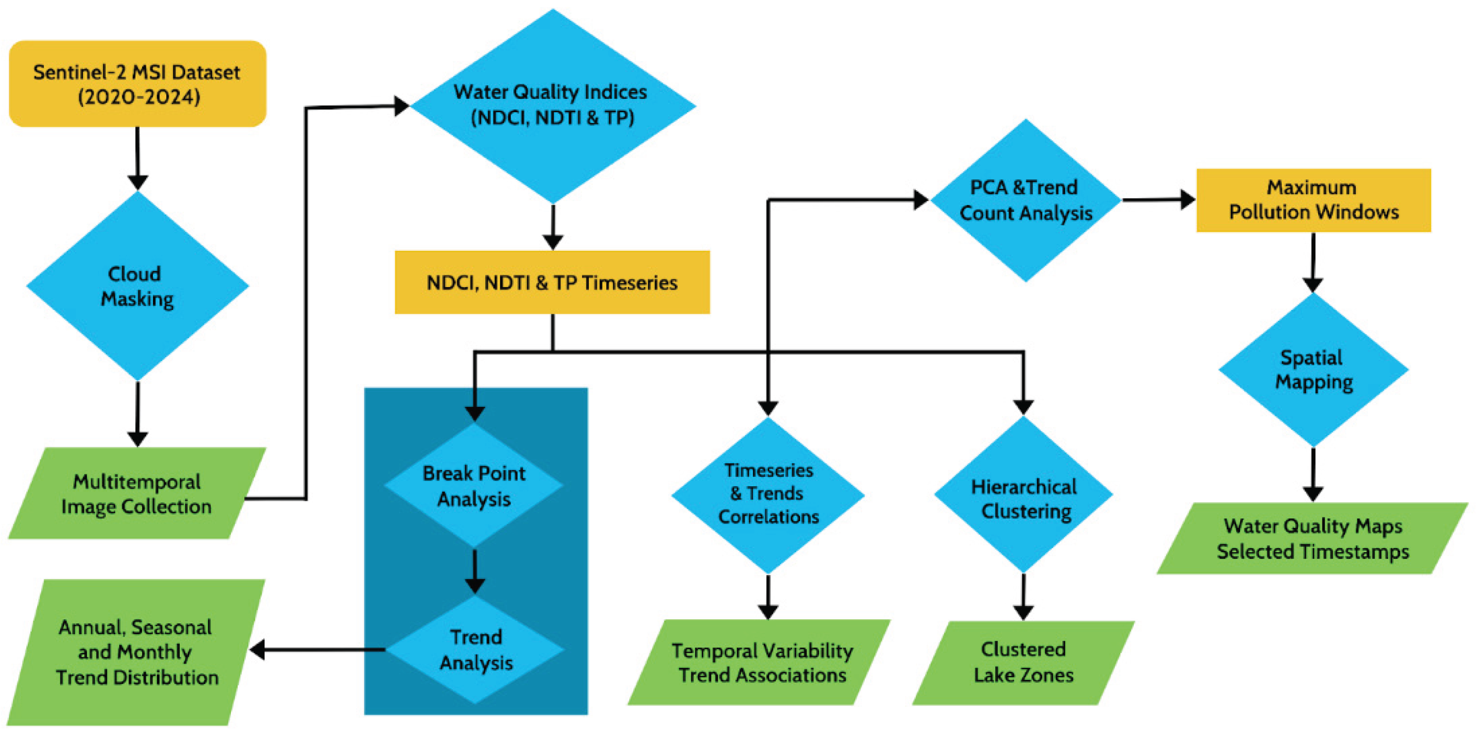
Figure 3.
Time series of NDCI (green), NDTI (orange), and TP (blue) across five regions of Horseshoe Lake from 2020 to 2024.
Figure 3.
Time series of NDCI (green), NDTI (orange), and TP (blue) across five regions of Horseshoe Lake from 2020 to 2024.

Figure 4.
Box-and-whisker plots showing the distribution of NDCI, NDTI, and TP values across the five regions of Horseshoe Lake. Colors indicate different regions: Region 1 = teal, Region 2 = orange, Region 3 = blue, Region 4 = pink, and Region 5 = green.
Figure 4.
Box-and-whisker plots showing the distribution of NDCI, NDTI, and TP values across the five regions of Horseshoe Lake. Colors indicate different regions: Region 1 = teal, Region 2 = orange, Region 3 = blue, Region 4 = pink, and Region 5 = green.
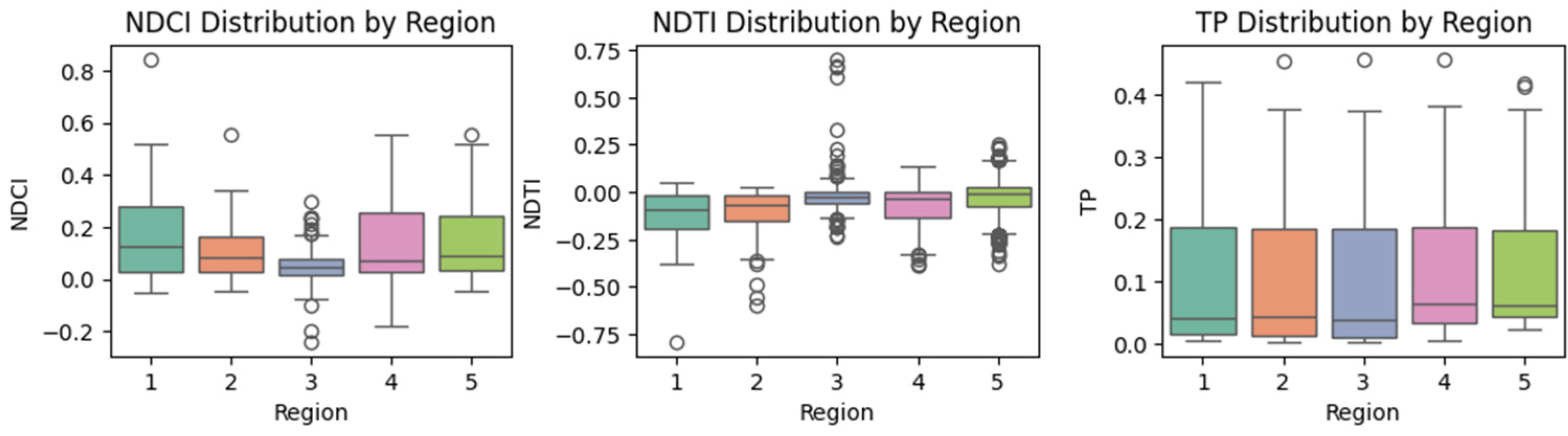
Figure 5.
Time series of NDCI for the five Horseshoe Lake regions with detected breakpoints and classified trend segments (2020–2024). Trend colors indicate direction: red = increasing, blue = decreasing, and black =non-significant. This color scheme is applied consistently to both the time-series trend segments (left panels) and the bar plots (right panels), where the bars summarize the relative proportion of each trend category across years, seasons, and months.
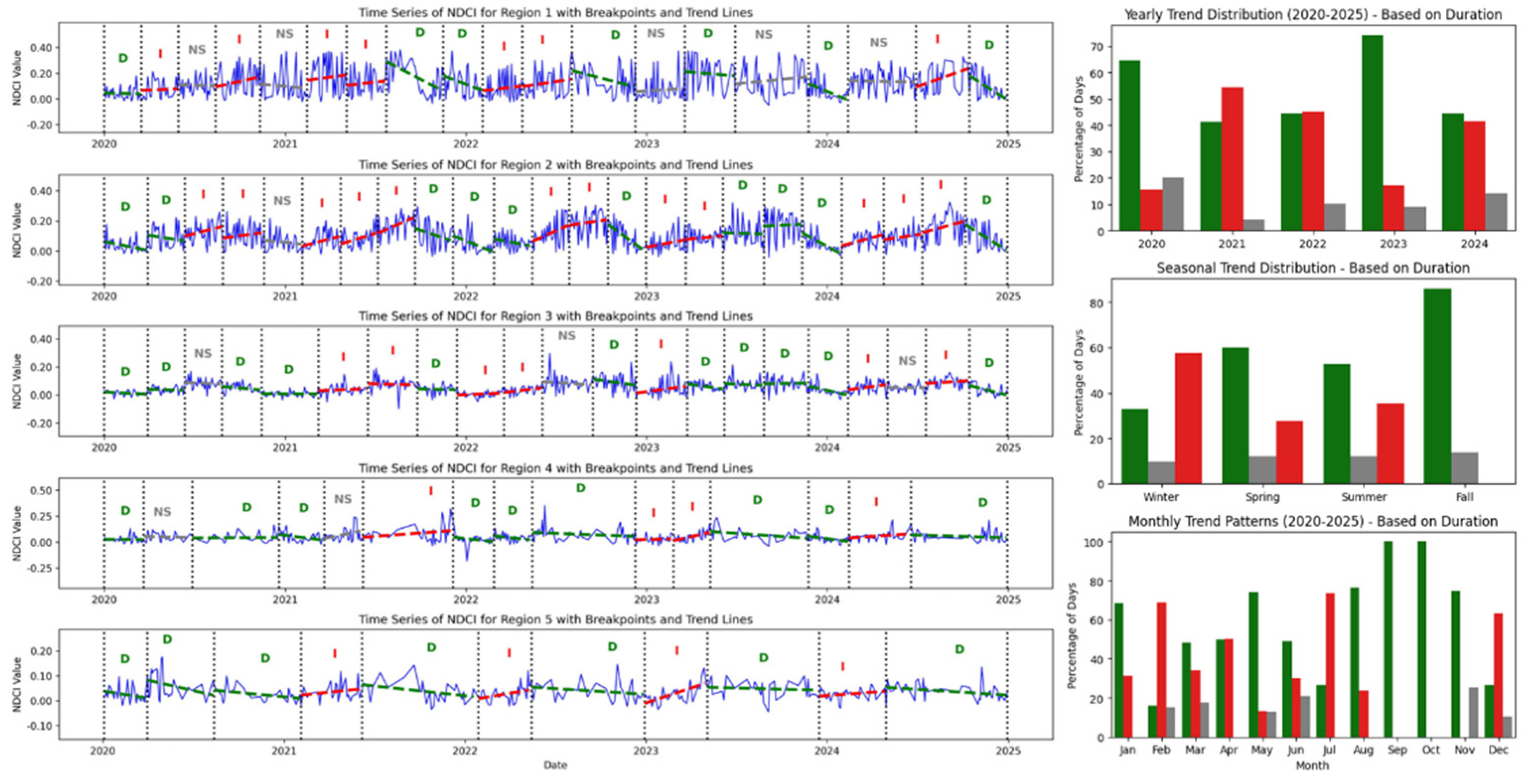
Figure 6.
Time series of NDTI for the five Horseshoe Lake regions with Breakpoints and Trend Lines from 2020 to 2024.
Figure 6.
Time series of NDTI for the five Horseshoe Lake regions with Breakpoints and Trend Lines from 2020 to 2024.
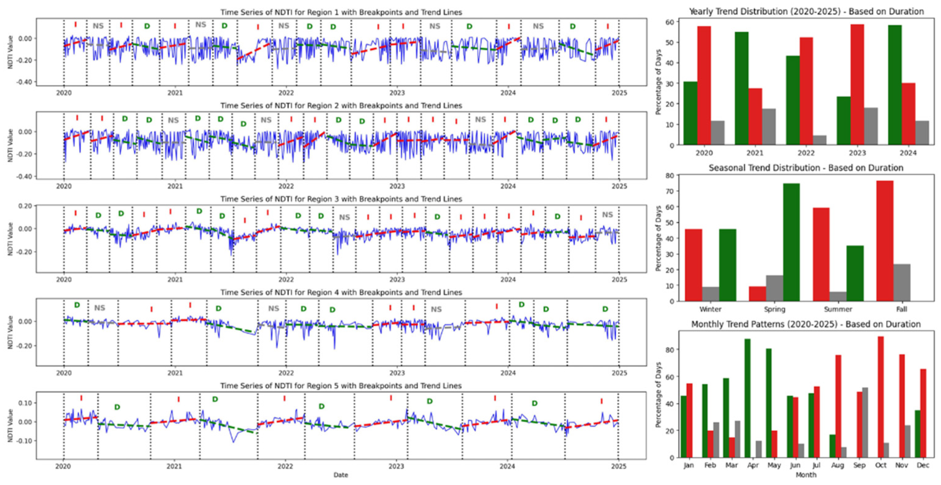
Figure 7.
Time series of TP for the five Horseshoe Lake regions with Breakpoints and Trend Lines from 2020 to 2024.
Figure 7.
Time series of TP for the five Horseshoe Lake regions with Breakpoints and Trend Lines from 2020 to 2024.
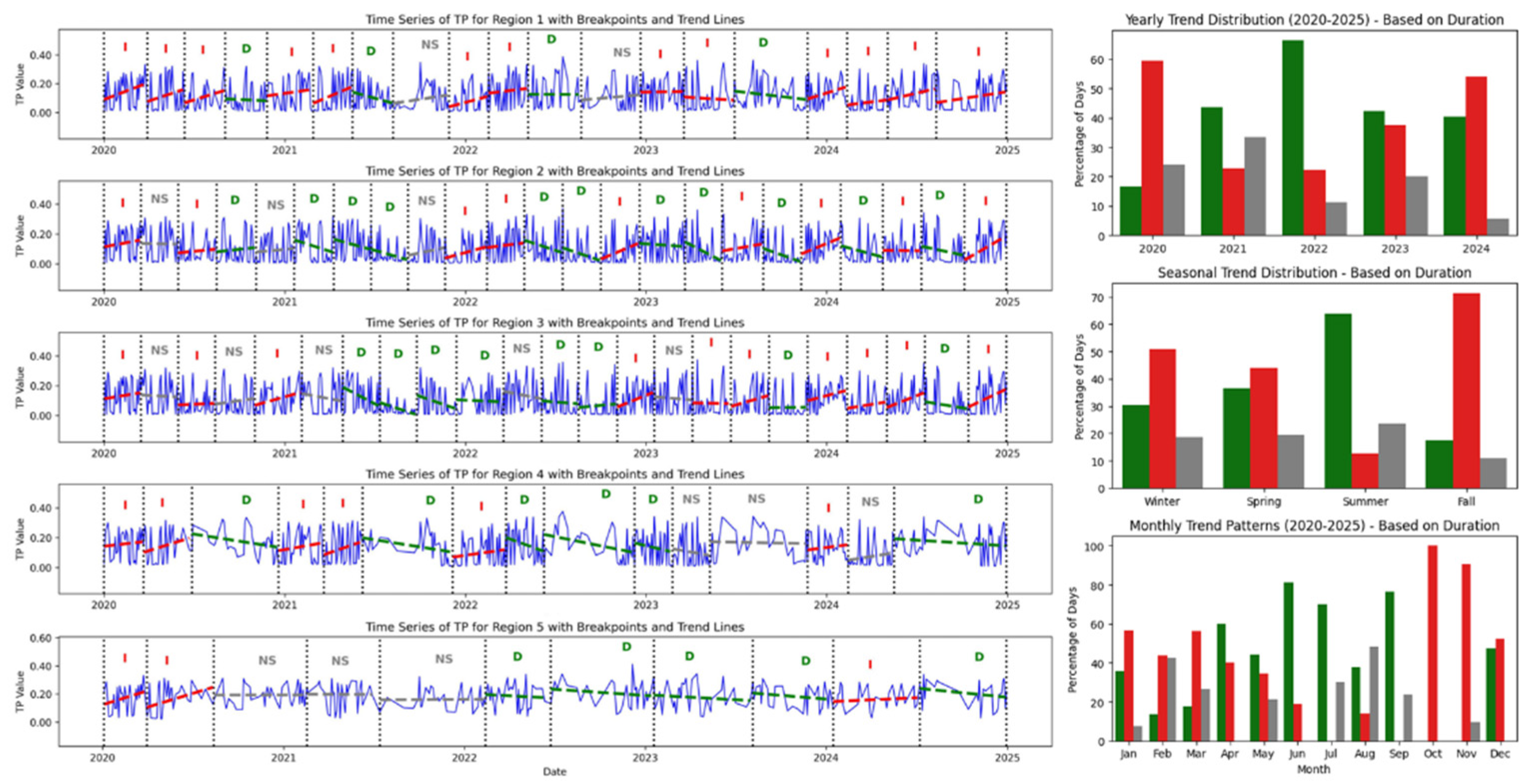
Figure 8.
Correlation matrices of NDCI, NDTI, and TP across five lake regions in Horseshoe Lake from 2020 to 2024. The top row shows Pearson correlation coefficients for raw time series values. The bottom row shows correlations based on segmented trend values.
Figure 8.
Correlation matrices of NDCI, NDTI, and TP across five lake regions in Horseshoe Lake from 2020 to 2024. The top row shows Pearson correlation coefficients for raw time series values. The bottom row shows correlations based on segmented trend values.
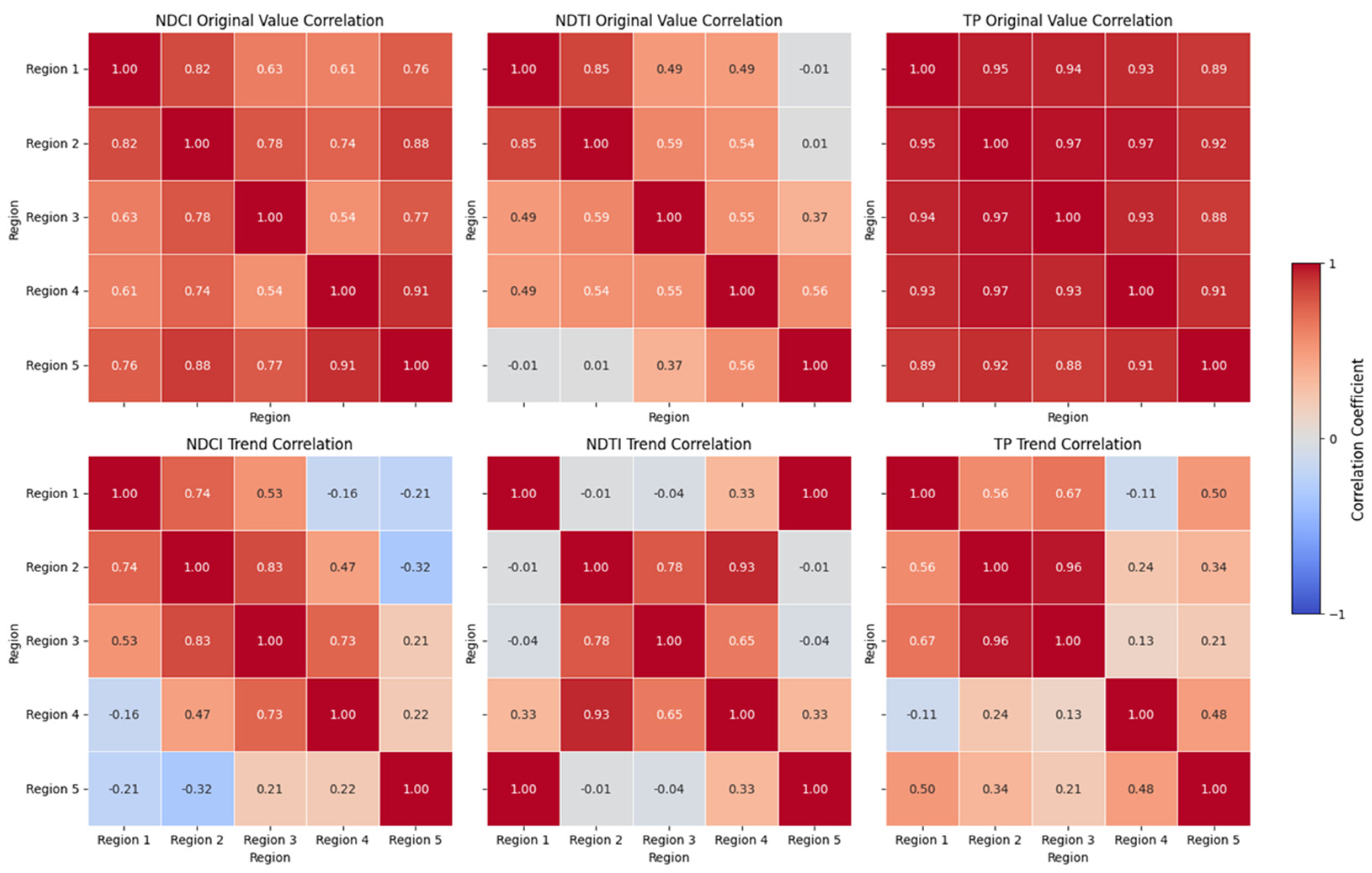
Figure 9.
Hierarchical clustering of HSL regions based on NDCI, NDTI, and TP (2020–2024).
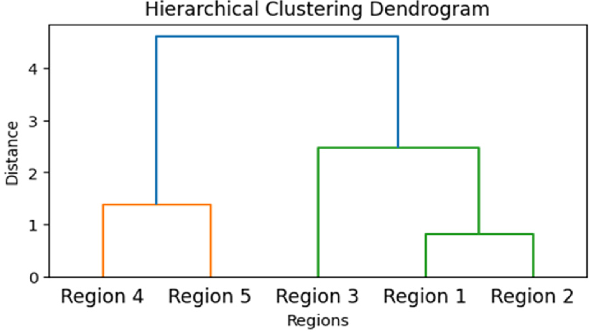
Figure 10.
Composite Pollution Metric (PC1) and Increasing Trend Segments Over Time (2020–2024), Including Explained Variance Ratio from K-PCA Analysis.
Figure 10.
Composite Pollution Metric (PC1) and Increasing Trend Segments Over Time (2020–2024), Including Explained Variance Ratio from K-PCA Analysis.
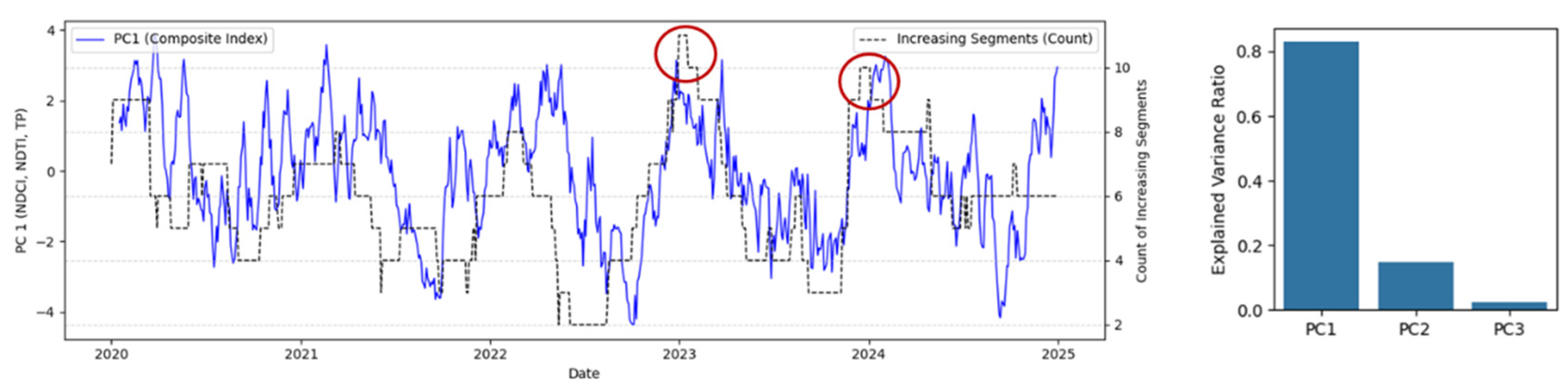
Figure 11.
Spatial distribution of NDCI, NDTI, and TP during the first high-pollution window (31 Dec 2022 – 15 Jan 2023).
Figure 11.
Spatial distribution of NDCI, NDTI, and TP during the first high-pollution window (31 Dec 2022 – 15 Jan 2023).
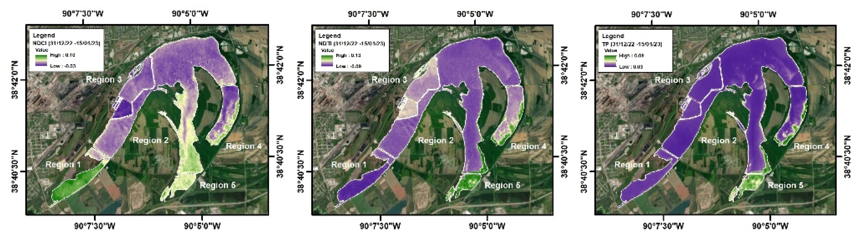
Figure 12.
Spatial distribution of NDCI, NDTI, and TP during the second high-pollution window (24 Nov 2023 – 10 Jan 2024).
Figure 12.
Spatial distribution of NDCI, NDTI, and TP during the second high-pollution window (24 Nov 2023 – 10 Jan 2024).
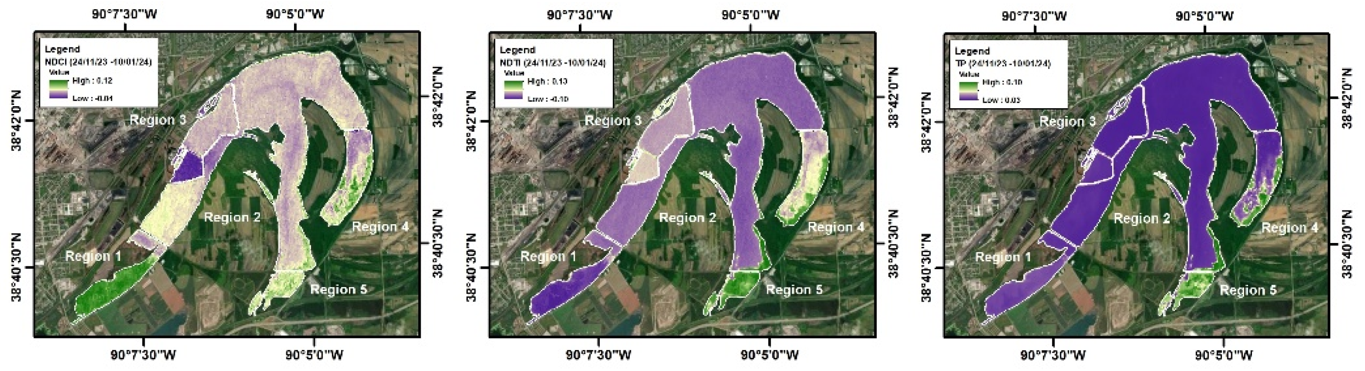
Figure 13.
Land Cover and Hydrological Context of Horseshoe Lake within the American Bottom.
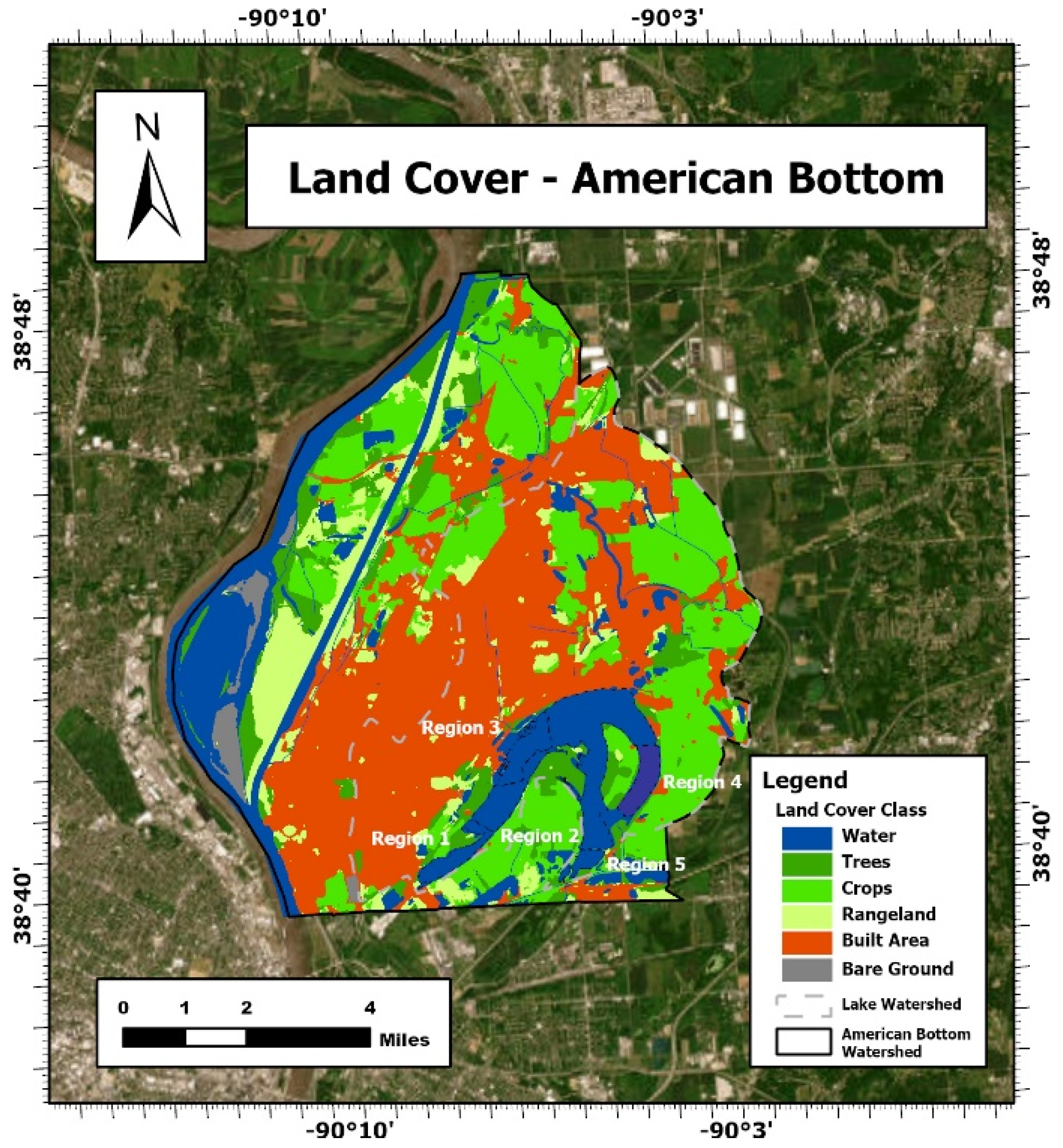

Table 1.
Sentinel-2 S2_SR_HARMONIZED Spectral Bands and Characteristics.
| Band Name |
Band Number |
Band Description |
Central Wavelength (nm) |
Spatial Resolution (m) |
| B1 | Band 1 | Coastal aerosol | 443 | 60 |
| B2 | Band 2 | Blue | 490 | 10 |
| B3 | Band 3 | Green | 560 | 10 |
| B4 | Band 4 | Red | 665 | 10 |
| B5 | Band 5 | Red edge 1 | 705 | 20 |
| B6 | Band 6 | Red edge 2 | 740 | 20 |
| B7 | Band 7 | Red edge 3 | 783 | 20 |
| B8 | Band 8 | NIR (Near-Infrared) | 842 | 10 |
| B8A | Band 8A | Narrow NIR | 865 | 20 |
| B9 | Band 9 | Water vapor | 945 | 60 |
| B11 | Band 11 | SWIR 1 (Short-Wave Infrared) | 1610 | 20 |
| B12 | Band 12 | SWIR 2 | 2190 | 20 |
| QA60 | - | Cloud mask bitmask | - | 60 |
Disclaimer/Publisher’s Note: The statements, opinions and data contained in all publications are solely those of the individual author(s) and contributor(s) and not of MDPI and/or the editor(s). MDPI and/or the editor(s) disclaim responsibility for any injury to people or property resulting from any ideas, methods, instructions or products referred to in the content. |
© 2025 by the authors. Licensee MDPI, Basel, Switzerland. This article is an open access article distributed under the terms and conditions of the Creative Commons Attribution (CC BY) license (http://creativecommons.org/licenses/by/4.0/).
Copyright: This open access article is published under a Creative Commons CC BY 4.0 license, which permit the free download, distribution, and reuse, provided that the author and preprint are cited in any reuse.


