
Submitted:
27 August 2025
Posted:
28 August 2025
You are already at the latest version
Abstract
The density of vehicles on the road is an important metric of the traffic state. It can be used to estimate traffic congestion, predict travel times, optimize traffic flow, implement dynamic routing strategies, etc. Thus, vehicle density estimation plays a critical role in traffic management. At the same time, vehicles connected via vehicle-to-everything ( V2X) technology can exchange information by broadcasting wareness messages (AMs), making them naturally suited to estimate vehicle density.
However, a vehicle might underestimate density due to the loss of some awareness messages from its neighbors. To address this, we propose a scheme that enables vehicles to locally estimate vehicle density based on the received AMs and the broadcast reliability of V2X. The scheme proposes an innovative method to estimate the ratio of the sensed vehicles to the total number of vehicles based on observed reliability metrics. Experimental results show that, compared with a method based solely on received messages, the proposed method improves the density estimation accuracy by up to 37% at an actual density of 0.28 Vehs/m, while not requiring additional communication overhead. We also present an example application of the estimated density, in which the Basic Safety Message (BSM) rate is dynamically adjusted.
Keywords:
Traffic management
; Density estimation
; V2X
; Awareness messages
; Reliability
1. Introduction
As the transportation industry advances, the growing number of vehicles enhances convenience for daily life but complicates traffic management, posing challenges to achieving safety, efficiency, and environmental sustainability [1,2]. In such a situation, enhancing the awareness capability of vehicles is the key to achieving advanced traffic management in Intelligence Transportation System (ITS). For an on-road vehicle, a fundamental requirement is awareness of the number of neighboring vehicles, or vehicle density. This awareness would directly influence the vehicle’s moving strategy and states, such as risk assessment, path selection, etc. [3,4]. At the same time, vehicle density is also an important factor that affects the performance of V2X, which could allow vehicles to communicate with each other and improve their awareness. For example, a higher vehicle density can lead to more interference, resulting in less reliable communication. Thus, vehicle density estimation also plays an important role in leveraging the capabilities of V2Xs. With an accurate estimation of vehicle density, the reliability of V2X and the vehicle awareness could be improved with proper optimization methods, such as adjusting the message rate based on the estimation [5].
Accurate estimation of vehicle density remains essential, as collecting high-quality traffic data is constrained by the high cost of infrastructure, limited sensor coverage, and potential inaccuracies introduced during data collection and transmission processes [6]. Numerous vehicle density estimation methods have been proposed, typically classified into two categories: infrastructure-based methods and infrastructure-free methods [7]. Infrastructure-based methods were first proposed and applied in traffic engineering, which rely on pre-installed cameras or sensors (such as inductive loop detectors, roadside radars, etc.) to collect traffic status information and then estimate vehicle density [8]. However, these methods suffer from drawbacks such as limited spatial coverage, high maintenance costs, and reduced real-time capabilities. Additionally, their accuracy can be affected by environmental conditions and sensor placement.
The emergence of V2X allows traffic status information to be collected through vehicular communication without pre-installed roadside infrastructures, which could make vehicle density estimation more flexible and timely. Connected vehicles can locally estimate vehicle density based on the received AMs, which are broadcast by vehicles and include information such as location, speed, and heading [9]. Typical examples include Society of Automotive Engineers (SAE)-standardized BSMs or European Telecommunications Standards Institute (ETSI)-standardized Cooperative Awareness Messages (CAMs). Since V2X works in an unreliable channel, these awareness messages can be lost due to channel fading and interference. Therefore, relying solely on received awareness messages might underestimate the actual number of nodes on the road.
However, a more precise vehicle density estimate can be achieved if the ratio of sensed vehicles to the total number of vehicles on the road can also be estimated. This paper proposes a local vehicle density estimation method based on the awareness messages received and their broadcast reliability. The host vehicle first computes Packet Reception Ratio (PRR) of the awareness messages from remote vehicles (neighbors of the host vehicle). Then the discrete PRR results are used to fit the Packet Reception Probability (PRP)-distance curve. Based on the fitted curve, the host vehicle employs a probabilistic method to derive an Application-layer metric Average Awareness Ratio (AAR), which is defined as the ratio of the number of vehicles detected to the actual number on the road (as defined in Section 4.3). Finally, the actual density of vehicles is estimated locally based on the number of vehicles detected and the metric AAR. No additional communication overhead is involved in physical (PHY) or Medium Access Control (MAC) layer since the proposed method uses only the received awareness messages to estimate vehicle density.
To calculate the AAR, we introduce another APP-layer reliability metric called Node Awareness Probability (NAP). NAP presents the probability that the host vehicle detects a given neighbor vehicle through the awareness messages received. Specifically, it is defined as the probability that the host vehicle will receive at least one AM from this neighbor vehicle during a specified observation period. NAP can be derived from PRP, which is normally expressed as a function of the packet transmission distance d [10] between the transmitter and the receiver. AAR can be computed by summing the NAP of neighbor nodes and dividing it by the total number of nodes (derived as shown in Eq. (12)). When focusing on the highway scenario, the distribution of vehicles on the road could be considered homogeneous, and the AAR could be computed by integrating NAP over the receiving distance.
The contributions of the paper are summarized as follows.
- a)
- A vehicle density estimation method is proposed, which can be carried out by host vehicles locally with the received awareness messages. No additional infrastructure and payloads are needed during the estimation. The proposed method is beneficial in providing accurate vehicle density for robust traffic management.
- b)
- Two APP-layer reliability metrics NAP and AAR are introduced. NAP presents the probability that the host vehicle senses a vehicle. While AAR represents the ratio of the number of sensed vehicles to the total number of nearby vehicles. Then, the vehicle density could be estimated based on the received awareness messages and the derived AAR;
- c)
- We present an awareness messages-based method to calculate PRR in V2X, fit PRP-distance function, and derive the APP-layer reliability metrics NAP and NAR using the probabilistic method;
- d)
- We conduct NS2 simulations under various vehicle densities to validate the accuracy of the proposed density estimation method. The results demonstrate that our method achieves higher accuracy than approaches relying solely on the number of sensed vehicles. Furthermore, although the application of the estimated density is beyond the scope of this paper, we still present an example in the context of congestion control.
The remainder of the paper is organized as follows: Section 2 introduces the related work on vehicle density estimation in vehicular networks. Section 3 presents the proposed framework of density estimation, system model, and assumptions. Section 4 describes the reliability evaluation of AM broadcasting. Section 4.4 introduces the density estimation. Section 5 gives the experimental settings and results. Section 6 concludes the paper.
2. Related Work
As described in Section 1, the traditional method of estimating the density of vehicles is the infrastructure-based method, which uses pre-installed equipment to count traffic status information. The commonly used equipment includes cameras, sensors such as inductive loop detectors, roadside radars, infrastructures, etc. [11,12,13,14]. The measurement coverage of the methods is limited since the cameras and sensors could not work in an area beyond their range and could not be widely deployed due to cost constraints [3,6]. The other limits of sensors include relatively short lifespans and high maintenance costs, which hinder their widespread adoption for traffic monitoring [8]. As for cameras, factors such as their height, resolution, distance from vehicles, and weather conditions can affect the quality of images and the accuracy of vehicle density estimation [8].
Recently, V2X-based strategies have been studied more extensively because vehicular communication enables a more flexible and timely collection of traffic information while eliminating the need for additional infrastructure deployment. Some approaches estimate vehicle density with self-defined observers and messages, referred to as the self-defined message-based method. For example, Shin et al. [3] proposed an algorithm to explore vehicle density based on probing packets transmitted by a vehicle sampler. The sampler broadcasts a HELLO message to the neighbors and counts the number of neighbors according to their REPLY messages. Florin et al. [15] proposed a method to estimate vehicle density on the highway in a privacy-preserving manner by counting and sharing the number of times vehicles pass each other.
Other approaches for vehicle density estimation were proposed by directly using awareness messages. In this category, Barrachina et al. [16] proposed a vehicle density estimation solution for urban scenarios based on the topology of the roadmap and the number of BSMs received by Road Side Units (RSUs), which is not suitable for fully autonomous networks. Other solutions are proposed to estimate vehicle density based on awareness messages broadcast between vehicles, which are completely suitable for autonomous mode and do not require the participation of RSUs. For example, the number of vehicles could be estimated by counting the number of message sources based on the received beacons [17,18] or the acknowledgment packets [19]. However, the impact of packet loss is not considered.
In summary, the self-defined message-based method increases the network load to a certain extent. The AM-based method uses inherent AMs, which neither increases the network load nor modifies the original protocol, making integration easy to achieve. However, the estimated density based solely on information in awareness messages represents the density of sensed vehicles, which may underestimate the actual vehicle density due to packet loss. Therefore, the reliability of AM broadcasting should also be considered to ensure a more accurate estimation of vehicle density. Existing literature also points out this issue [19,20,21,22], however, no solutions are provided for mapping the number of sensed vehicles to the total number of vehicles.
3. Proposed Framework, System Model and Assumptions
3.1. Proposed Framework for Vehicle Density Estimation
The proposed vehicle density estimation could be performed locally on each vehicle in a distributed manner. For clarity, three kinds of vehicles are defined in this paper:
- Host vehicle is the vehicle that estimates the vehicle density. And it is marked as ;
- Remote vehicles are defined as the neighbors of the . The i-th remote vehicle is marked as ;
- Sensed vehicle is defined as a remote vehicle from which the host vehicle receives at least one AM within the observation period. The i-th sensed vehicle is marked as .
Figure 1 illustrates the proposed density estimation procedure performed in the host vehicle. After receiving awareness messages in a predefined observation period , the host vehicle calculates two metrics — the number of sensed vehicles and the AAR — to estimate vehicle density. Since awareness messages are generated and broadcast periodically by each vehicle, the host vehicle calculates the PRR for each sensed vehicle based on the predefined packet generation interval and the number of messages received. Next, the PRP-distance curve could be fitted using the discrete PRR values. If the fitted PRP function does not follow the decreasing trend, or if there are inflection points, the PRR value at long distances should be reconstructed, and then refit the PRP-distance function. The fitted PRP-distance function is used to calculate NAP and AAR. On this basis, the vehicle density could be estimated.
3.2. System Model and Assumptions
Figure 2(a) illustrates connected vehicles in a highway scenario featuring several lanes in both directions. The host vehicle receives awareness messages from remote vehicles within its communication range . Since the communication range (normally hundreds of meters) is much greater than the road width, the highway could be abstracted into a one-dimensional (1-D) line as shown in Figure 2(b), and the vehicles could be represented as dots on the line. Besides, the following assumptions are given.
- a)
- Vehicles are distributed homogeneously on the highway, with a real vehicle density ;
- b)
- All vehicles are equipped with the same on-board wireless transmission devices, which means the technology penetration rate is 100%;
- c)
- All devices on the vehicles have same configurations, including transmit power , data rate , and so on;
- d)
- The received power with distance d away from the transmitter follows a fading/shadowing channel model, which could be expressed as follows [23]:where is the path loss. is a a random gain variable representing the effects of fading and shadowing, characterized by the Probability Density Function (PDF) of the power : .
- e)
- A deterministic communication range is assumed, where [23], and is the receiving power threshold. For Nakagami fading, we havewhere is the reference distance, is the path loss exponent, and is a dimensionless constant in the path loss law determined by the carrier frequency f and the reference distance for the antenna far field, c is the speed of light.
4. Broadcast Reliability and Vehicle Density Estimation
The density of the sensed vehicles could be estimated based solely on the received awareness messages. In this section, the broadcast reliability metric AAR is introduced, defined as the ratio of the number of sensed vehicles to the total number of vehicles. Incorporating this metric allows the vehicle density estimate to be further refined with improved accuracy.
4.1. Packet Reception Ratio (PRR) Estimation
PRP is a link-level reliability metric defined as the probability that a packet from the transmitter is received successfully by the receiver . In contrast, PRR refers to the ratio of the number of packets successfully received by to the total number of packets transmitted by . PRR is a statistical metric and serves as an empirical estimate of PRP, reflecting its observed value through measurements or simulations:
where is the total number of packets transmitted by the remote vehicles, and is the number of packets received successfully by the host vehicle.
4.1.1. Pairwise PRR
The pairwise refers specifically to the case where the remote vehicle acts as the transmitter and the host vehicle as the receiver. According to the definition of PRR, the host vehicle can locally compute based on the awareness messages received from , as follows:
where denotes the expected number of packets broadcast by the remote vehicle during the host vehicle’s observation period , is the number of packets successfully received out of the total packets transmitted.
If the awareness messages are transmitted periodically, can be estimated by:
where is the message rate. It should be noted that even if the message rate is not constant, the host vehicle can also estimate by tracking the sequence numbers of the awareness messages [24].
4.1.2. Observation Distances
Taking the host vehicle as the reference point, the highway is divided into multiple segments, and the distance from the center of each segment to the host vehicle is referred to as the observation distance. The j-th observation distance is given by,
where is the total number of segments in front of or behind the host vehicle, is the segment distance increment, and is the communication range.
4.1.3. PRR Estimation over Observation Distances
The distance between the host vehicle and the remote vehicle is denoted as the receiving distance . The host vehicle can compute based on the location information included in the received awareness messages. The average PRR at the j-th observation distance can be calculated as:
where k is the number of vehicles located within the road segment .
4.1.4. PRP-Distance Function Fitting
After each observation period , the host vehicle can calculate m average PRRs at different observation distances. Typically, the number m does not exceed the total number of observation distances (), since no remote vehicles may be located at certain distances under normal conditions.
To fit the m discrete PRR-distance points into a continuous PRP-distance curve, the Savitzky-Golay filter is used for smoothing and denoising, followed by a polynomial fitting process (as shown in lines of Algorithm 1). Meanwhile, the effectiveness of the fitting is quantified by the Sum of Squared Errors (SSE):
where is the fitted PRP-distance function.
Ideally, the PRP-distance function is monotonically decreasing. However, under poor channel conditions, the calculated average PRRs may exhibit non-monotonic behavior with respect to distance. This is because, for some vehicles, all of their awareness messages are lost, making them unsensed. As a result, the denominator (that is, the number of packets expected by the host vehicle) in Eq. (7) is smaller than the actual number, while the numerator remains the same as the actual situation, thus overestimating PRR.
The function would be refitted if an inflection point is detected based on the slope. Since PRRs should decrease with receiving distances, the corresponding point is the inflection point when the slope starts to change from negative to positive. Before refitting the , some PRR-distance points would be reconstructed first, as described in the following steps (also see lines in Algorithm 1).
- a)
- Among the m discrete PRR-distance points, the index of the inflection point is denoted by ;
- b)
- The index of a specific point is marked as if the NAPs derived from the subsequent points no longer meet the quality of service (QoS) requirement, which is a threshold (e.g., 99.9%);
- c)
- Another PRR-distance point is marked as by Eq. (9).where is the index of the last PRR-distance point;
- d)
- The PRRs of the points with indices greater than are reconstructed using Eq. (10):where s is the slope calculated from two PRR-distance points with indices and , and are the PRR and distance of the point .
Finally, the PRP-distance function would be refitted using the reconstructed PRRs (line 14 of Algorithm 1).
| Algorithm 1 PRPFunctionFitting() |
|
4.2. Node Awareness Probability (NAP) Estimation
NAP refers to the probability that a remote vehicle could be sensed by the host vehicle, which is defined as the probability that at least one packet from the remote vehicle is received by the host vehicle within the given observation period [25]. NAP could be calculated as follows:
where is the message rate, d is the distance between the transmitter and receiver, is the observation period.
4.3. Average Awareness Ratio (AAR) Estimation
AAR is defined as the proportion of the sensed vehicles to the total number of remote vehicles within a given distance d from the host vehicle. AAR could be computed as follows:
where is the observation period, is the vehicle density. With the first assumption that vehicles are distributed homogeneously, the real vehicle density could be considered constant, and Eq. (12) could be rewritten as:
4.4. Density Estimation
Based solely on the received AMs, the host vehicle can estimate the vehicle density using the following expression:
where denotes the number of sensed vehicles within the communication range of the host vehicle. To enhance this estimate, the metric AAR can be incorporated, yielding a refined vehicle density:
5. Experiments
We conducted a series of experiments to evaluate the proposed density estimation method. In these experiments, SUMO was used for traffic simulation, while NS2 was employed for network simulation. Traffic snapshots at varying densities were captured to validate the effectiveness of the proposed approach. The following sections provide a detailed description of the experimental setup and results.
5.1. Experiment Settings
5.1.1. Traffic Scenario
We adopt the traffic simulation software SUMO to generate mobility traffic on a two-lane, two-way highway road. Each lane is 5 km long and 3.2 meters wide. A total of 14 traffic scenarios are created by varying the number of vehicles on the road from 100 to 1400, in increments of 100.
5.1.2. Communication Settings
In the experiment, NS2 (version 2.35) is used to simulate V2X based on IEEE 802.11p in the highway scenario. The Nakagami channel fading model is employed to characterize the wireless channel conditions [23]. The observation period is set as . 25 observation distances are set from 10 m to 490 m with a step size of . The other communication parameters are summarized in Table 1.
Two kinds of PRR are calculated. One is regarded as the real PRR, evaluated according to the definition of PRR, that is, calculating the ratio of the number of successfully received awareness messages and the total number of awareness messages sent in each link and then averaging. The other is the estimated PRR over observation distances calculated by Eq. (7). Based on the estimated PRRs at the host vehicle, PRP-distance function is fitted according to the Algorithm 1. NAP and AAR are further given.
5.2. Experiment Results
5.2.1. PRP/NAP Estimation in Different Densities
The estimation results corresponding to the actual vehicle densities ranging from 0.02 Vehs/m to 0.18 Vehs/m are illustrated in Figure 3, Figure 4, Figure 5 and Figure 6. Each figure includes two subplots:
In subplot (a), the dashed line represents the real values of PRRs, the dots indicate the PRRs estimated by Eq. (7) on the host vehicle, the solid line corresponds to the fitted PRP-distance curve according to the measured PRRs.
In subplot (b), the dashed line indicates the NAP calculated from the actual PRRs, while the dots present the NAP derived from the fitted PRP-distance curve.
As shown in Figure 3 to Figure 6, the actual PRR decreases with increasing receiving distance due to greater signal attenuation and a higher probability of packet loss. Additionally, for a given receiving distance, the actual PRR declines as the vehicle density increases, since higher vehicle density leads to greater interference and consequently more severe packet loss. Furthermore, the obtained APP-layer metric, NAPs, closely matches the actual values, demonstrating the feasibility of our proposed method for estimating NAP.
5.2.2. Inflection Point Analysis
Figure 6 also shows the results from a fitted PRP-distance curve where the inflection point (abbreviated as inf. pt. in figures) is retained. The estimated values closely match the actual values for distances below 300 m; however, at longer distances, the estimates exceed the actual values. Notably, the PRP/NAP initially decreases but begins to increase beyond 400 m, indicating an inflection point in the fitted PRP-distance curve. This trend deviates from the expected monotonic decline typically observed under real conditions.
The inconsistency at longer distances arises from the fact that the host vehicle fails to receive any awareness messages from some remote vehicles. Figure 7 presents the number of sensed vehicles according to the awareness messages received within each 10 m receiving distance segment, up to the maximum transmission range . As illustrated, the host vehicle accurately estimates the number of vehicles within 400 m. However, beyond this distance, the number of sensed vehicles falls short of the actual count. This phenomenon occurs because, as the distance increases, the probability of successfully receiving a packet decreases due to higher path loss and interference, leading to more frequent packet losses. When remote vehicles are not sensed by the host vehicle, the PRR is overestimated, since the denominator in Eq. (7) becomes smaller than the true number of vehicles. In general, higher vehicle density and longer distances lead to more severe packet losses caused by interference and channel fading, thereby making the estimation error more significant.
Therefore, when there is no inflection point in the fitted PRP-distance function, it can be used directly to compute AAR and subsequently evaluate the vehicle density. However, if an inflection point is present, the PRP-distance function must be refitted to improve accuracy. As shown in Figure 6, the refitted PRP-distance function with the inflection point eliminated, along with the estimated NAP, exhibits a consistently decreasing trend concerning the receiving distance, aligning with the expected behavior.
5.2.3. The Estimated Vehicle Density
Figure 8 compares the actual density and two types of estimated density of the vehicle. The results indicate that the density estimated solely from awareness messages (see star markers), as described by Eq. (14), is accurate when the actual density is below 0.12 Vehs/m. However, the estimation error increases noticeably as the density increases. In contrast, the density estimated incorporating AAR (see empty square markers), as defined in Eq. (15), is more accurate.
Furthermore, the accuracy of vehicle density estimation can be slightly improved by receiving and fusing reliability metrics estimated and shared by other vehicles via wireless communication (see the filled square markers). This collaborative approach would enhance the estimation of AAR and vehicle density; however, it can also introduce additional communication overhead.
The accuracy of the estimated density is computed as follows:
where represents the actual vehicle density, and is the estimated density, which may refer to either or , as derived in Eq. (14) and Eq. (15), respectively.
Table 2 compares the accuracy of two types of estimated vehicle density. The proposed AM-AAR-based density estimation method improves the accuracy by 8%, increasing it from 84% to 92% when the actual density is 0.16 Vehs/m. The accuracy improvement is even more significant at higher density, with a 37% increase, from 58% to 95%, when the actual density is 0.28 Vehs/m. Experimental results demonstrate that this estimation method is feasible and does not incur additional communication overhead.
It is worth noting that the number of sensed vehicles may differ from the number of vehicles whose AMs are successfully received, as the pilot or header of an AM can be detected even if the full message fails to decode correctly. Taking this discrepancy into account could further enhance the accuracy of the density estimation.
5.2.4. The Impact of Vehicle Speed on Estimation Accuracy
Table 2 also gives the vehicle speed corresponding to the vehicle density in the experiments. Their relationship could be described as Greenshields model [25]. Furthermore, the analysis of Table 2 reveals a clear relationship between vehicle speed and estimated vehicle density accuracy, with speed decreasing from 21.7 m/s to 9.4 m/s as actual vehicle density increases from 0.16 to 0.28 vehicles per meter. The AM-based density estimation method shows a significant decline in accuracy from 0.84 to 0.58, likely due to its reduced effectiveness in high-density, low-speed scenarios where communication or spacing measurements are disrupted by congestion.
In contrast, the AM-AAR-based method maintains a higher and more stable accuracy range of 0.89 to 0.95, demonstrating greater robustness across varying densities and speeds. This suggests that the AM-AAR approach, possibly through adaptive adjustments, better handles the challenges of low-speed, high-density traffic, making it a preferable choice for accurate vehicle density estimation in such conditions.
5.2.5. Apply the Estimated Density to Adjust AM Rate
Herein, a potential application of the estimated vehicle density is illustrated. To alleviate communication congestion in high-density traffic scenarios and reduce data packet collisions, various congestion control mechanisms adjust transmission parameters based on vehicle density. In this context, we adopt the idea of the congestion control scheme defined in SAE J2945/1, in which the message rate is dynamically adjusted according to vehicle density [5]. According to the standard, the message transmission interval is set based on the estimated density as follows:
where B is the vehicle density coefficient (default: ), , and is the maximum allowed transmission interval.
Figure 9 compares the estimated AAR before and after adjusting the message rate (or the message transmission interval). The default message rate is set as . The results show that AAR improves with the adjusted message rate, and more than 90% of the vehicles can be sensed by the host vehicle when the density is 0.28 Vehs/m.
6. Conclusion
The main contribution of this paper is the development of a local vehicle density estimation method based on received awareness messages and the reliability metric AAR. The proposed approach offers several advantages. First, it enables real-time processing of density estimates. Second, it achieves high estimation accuracy, even under high vehicle densities. Compared to methods that are based solely on information from received awareness messages, the proposed method improves estimation accuracy by 8% and 37% at actual density of 0.16 Vehs/m and 0.28 Vehs/m, respectively. Third, the method is easy to implement, as it relies only on standard awareness messages without requiring any additional message fields.
In the future, we will apply the method to more scenarios to provide more insights for traffic density estimation, such as, Non-Line-Of-Sight (NLOS) scenario, intersection scenario, etc. Although many excellent density estimation methods have been given, this method is different from previous methods and can be an optional density estimation solution to solve several problems in traffic management.
Lastly, it is noteworthy that our vehicle density estimation process simultaneously incorporates reliability estimation. Given that different safety applications have distinct reliability requirements and parameter adjustments consume energy, the reliability estimation results guide the system in selecting optimal timing for parameter tuning. We plan to further explore this aspect in subsequent publications.
Author Contributions
Conceptualization, Z. L.; methodology, X. W. and Z. W.; software, X. W. and Z. L.; validation, X. W., and Z. L.; formal analysis, Z. W.; investigation, Z. W.; data curation, Z. W.; writing—original draft preparation, Z. L.; writing—review and editing, X. M., A. B.; visualization, X. W.; supervision, X. M., A. B., and J. Z.; project administration, Z. L.; funding acquisition, Z. L.. All authors have read and agreed to the published version of the manuscript.
Funding
This research was funded by the Basic Scientific Research Funds of Universities of Heilongjiang Province grant number 2023-KYYWF-1485.
Institutional Review Board Statement
Not applicable.
Informed Consent Statement
Not applicable.
Data Availability Statement
Not applicable.
Conflicts of Interest
The authors declare no conflicts of interest.
References
- Majumdar, S.; Subhani, M.M.; Roullier, B.; Anjum, A.; Zhu, R. Congestion prediction for smart sustainable cities using IoT and machine learning approaches. Sustainable Cities and Society 2021, 64, 102500. [Google Scholar] [CrossRef]
- Lu, J.; Li, B.; Li, H.; Al-Barakani, A. Expansion of city scale, traffic modes, traffic congestion, and air pollution. Cities 2021, 108, 102974. [Google Scholar] [CrossRef]
- Shin, C.S.; Lee, J.; Lee, H. Infrastructure-Less Vehicle Traffic Density Estimation via Distributed Packet Probing in V2V Network. IEEE Trans. Veh. Tech. 2020, 69, 10403–10418. [Google Scholar] [CrossRef]
- Al-Sobky, A.S.A.; Mousa, R.M. Traffic density determination and its applications using smartphone. Alexandria Engineering Journal 2016, 55, 513–523. [Google Scholar] [CrossRef]
- Shimizu, T.; Cheng, B.; Lu, H.; Kenney, J. Comparative Analysis of DSRC and LTE-V2X PC5 Mode 4 with SAE Congestion Control. In Proceedings of the 2020 IEEE Vehicular Networking Conference (VNC); 2020; pp. 1–8. [Google Scholar] [CrossRef]
- Zhang, J.; Mao, S.; Yang, L.; Ma, W.; Li, S.; Gao, Z. Physics-informed deep learning for traffic state estimation based on the traffic flow model and computational graph method. Information Fusion 2024, 101, 101971. [Google Scholar] [CrossRef]
- Darwish, T.; Abu Bakar, K. Traffic density estimation in vehicular ad hoc networks: A review. Ad Hoc Networks 2015, 24, 337–351. [Google Scholar] [CrossRef]
- Lin, Y.; Xiao, N. Identifying high-accuracy regions in traffic camera images to enhance the estimation of road traffic metrics: a quadtree-based method. Transportation research record 2022, 2676, 522–534. [Google Scholar] [CrossRef]
- Zhao, J.; Wang, Y.; Lu, H.; Li, Z.; Ma, X. Interference-Based QoS and Capacity Analysis of VANETs for Safety Applications. IEEE Trans. Veh. Technol. 2021, 70, 2448–2464. [Google Scholar] [CrossRef]
- Li, Z.; Wu, X.; Li, X.; Ma, X. Interference-Based Reliability and Capacity Analysis for IEEE 802.11 Broadcast Ad-Hoc Networks on the Highway. In Proceedings of the Proceedings of the 11th International Conference on Vehicle Technology and Intelligent Transport Systems (VEHITS 2025), Porto, Portugal, Apr. 2025; pp. 520–528. [CrossRef]
- Wang, J.; Huang, Y.; Feng, Z.; Jiang, C.; Zhang, H.; Leung, V.C.M. Reliable Traffic Density Estimation in Vehicular Network. IEEE Trans. Veh. Technol. 2018, 67, 6424–6437. [Google Scholar] [CrossRef]
- Hu, Z.; Lam, W.H.; Wong, S.; Chow, A.H.; Ma, W. Turning traffic surveillance cameras into intelligent sensors for traffic density estimation. Complex & Intelligent Systems 2023, 9, 7171–7195. [Google Scholar] [CrossRef]
- Sankaranarayanan, M.; Mala, C.; Jain, S. Traffic density estimation for traffic management applications using neural networks. International Journal of Intelligent Information Technologies (IJIIT) 2024, 20, 1–19. [Google Scholar] [CrossRef]
- Zhang, Y.; Jia, R.S.; Yang, R.; Sun, H.M. DSNet: A vehicle density estimation network based on multi-scale sensing of vehicle density in video images. Expert Systems with Applications 2023, 234, 121020. [Google Scholar] [CrossRef]
- Florin, R.; Olariu, S. Real-Time Traffic Density Estimation: Putting on-Coming Traffic to Work. IEEE Trans. Intell. Transp. Syst. 2023, 24, 1374–1383. [Google Scholar] [CrossRef]
- Barrachina, J.; Fogue, M.; Garrido, P.; Martinez, F.J.; Cano, J.C.; Calafate, C.T.; Manzoni, P. Assessing vehicular density estimation using vehicle-to-infrastructure communications. In Proceedings of the IEEE 14th International Symposium on WoWMoM, June 2013; pp. 1–3. [Google Scholar] [CrossRef]
- Yao, Y.; Zhou, X.; Zhang, K. Density-Aware Rate Adaptation for Vehicle Safety Communications in the Highway Environment. IEEE Communications Letters 2014, 18, 1167–1170. [Google Scholar] [CrossRef]
- Chen, R.; Chen, B. Traffic State Estimation Using Basic Safety Messages Based on Kalman Filter Technique. In Proceedings of the 2024 IEEE 6th International Conference on Civil Aviation Safety and Information Technology (ICCASIT). IEEE; 2024; pp. 1601–1610. [Google Scholar]
- Rawat, D.B.; Yan, G.; Popescu, D.C.; Weigle, M.C.; Olariu, S. Dynamic Adaptation of Joint Transmission Power and Contention Window in VANET. In Proceedings of the 2009 IEEE 70th Vehicular Technology Conference Fall; 2009; pp. 1–5. [Google Scholar] [CrossRef]
- Mertens, Y.; Wellens, M.; Mahonen, P. Simulation-Based Performance Evaluation of Enhanced Broadcast Schemes for IEEE 802. In 11-Based Vehicular Networks. In Proceedings of the VTC Spring 2008 - IEEE Vehicular Technology Conference; 2008; pp. 3042–3046. [Google Scholar] [CrossRef]
- Stanica, R.; Chaput, E.; Beylot, A.L. Local density estimation for contention window adaptation in vehicular networks. In Proceedings of the 2011 IEEE 22nd International Symposium on Personal, Indoor and Mobile Radio Communications; 2011; pp. 730–734. [Google Scholar] [CrossRef]
- Bauza, R.; Gozalvez, J. Traffic congestion detection in large-scale scenarios using vehicle-to-vehicle communications. Journal of Network and Computer Applications 2013, 36, 1295–1307. [Google Scholar] [CrossRef]
- Ma, X.; Trivedi, K.S. SINR-Based Analysis of IEEE 802.11p/bd Broadcast VANETs for Safety Services. IEEE Trans. Netw. Service Manag. 2021, 18, 2672–2686. [Google Scholar] [CrossRef]
- On-Board System Requirements for V2V Safety Communications. Technical Report SAE J2945/1_202004, 2020. Revised April 2020, Issued March 2016.
- Li, Z.; Wang, Y.; Zhao, J. Reliability Evaluation of IEEE 802.11p Broadcast Ad Hoc Networks on the Highway. IEEE Trans. Veh. Technol. 2022, 71, 7428–7444. [Google Scholar] [CrossRef]
Figure 1.
Density estimation procedure of our proposed method
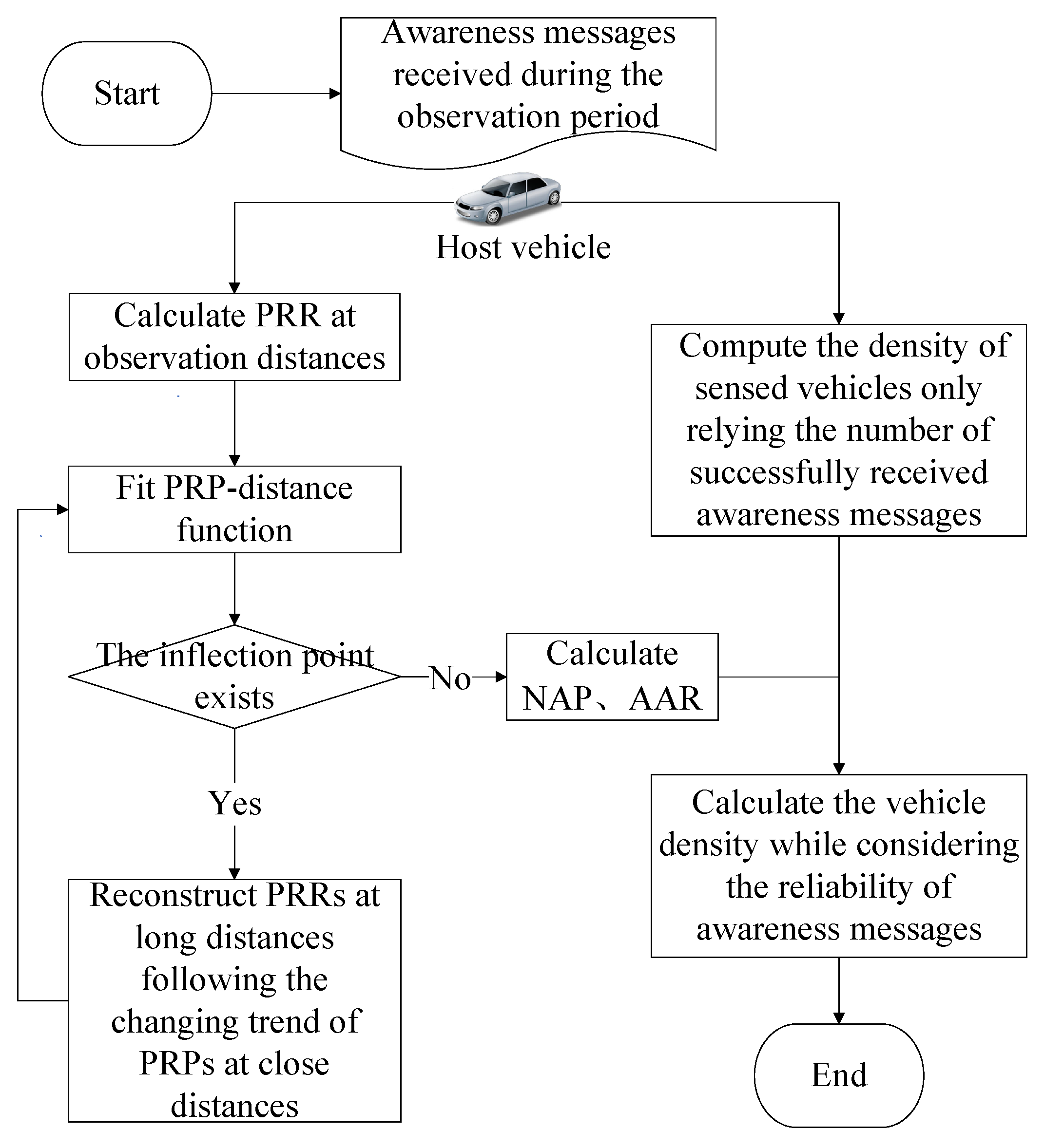
Figure 2.
Highway scenario and abstract model
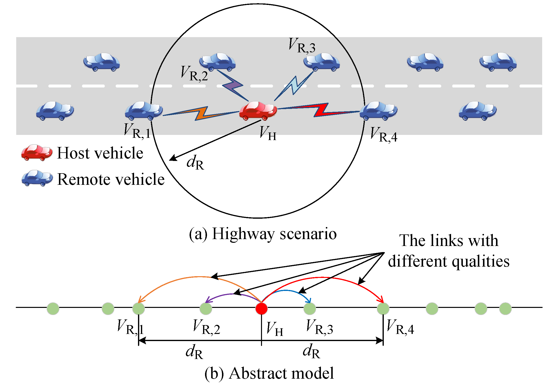
Figure 3.
Comparisons of actual and estimated reliability metrics ( Vehs/m).
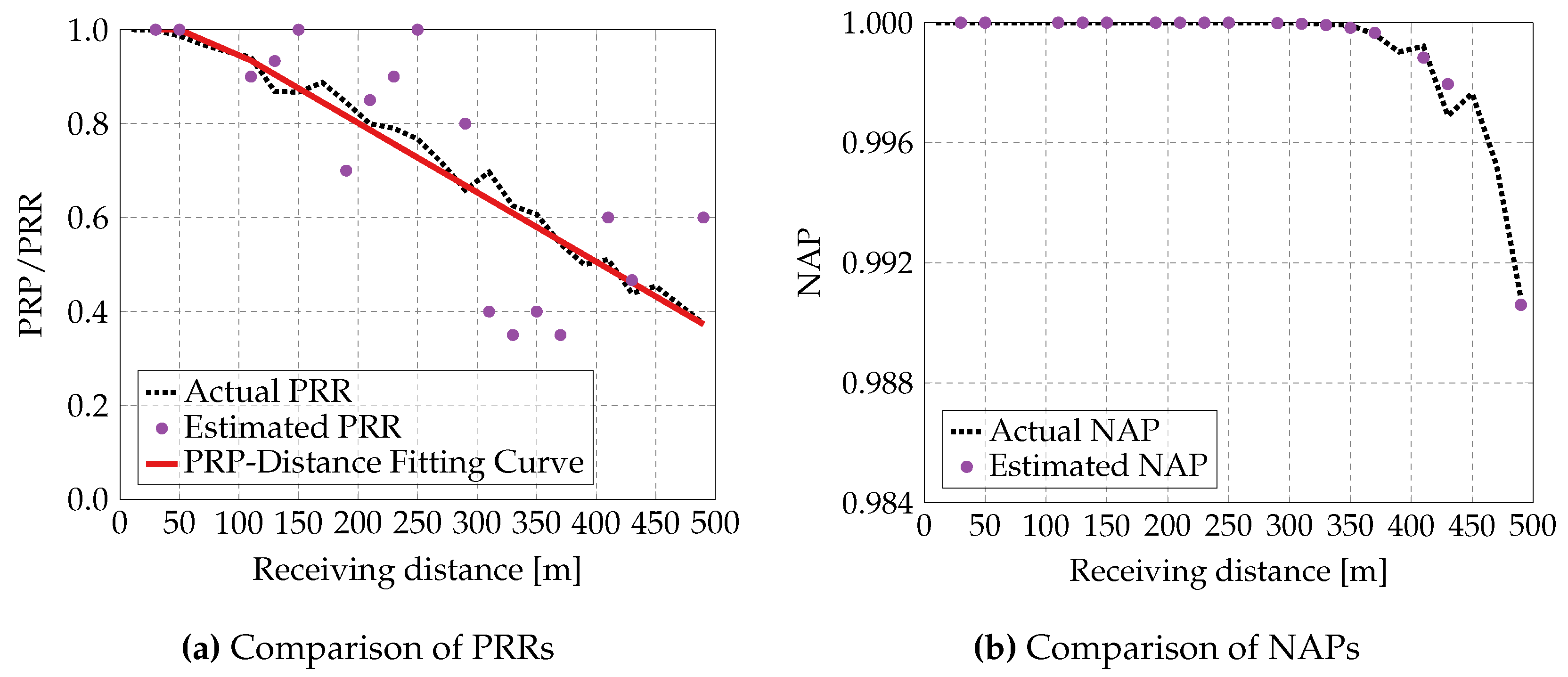
Figure 4.
Comparisons of actual and estimated reliability metrics ( Vehs/m).
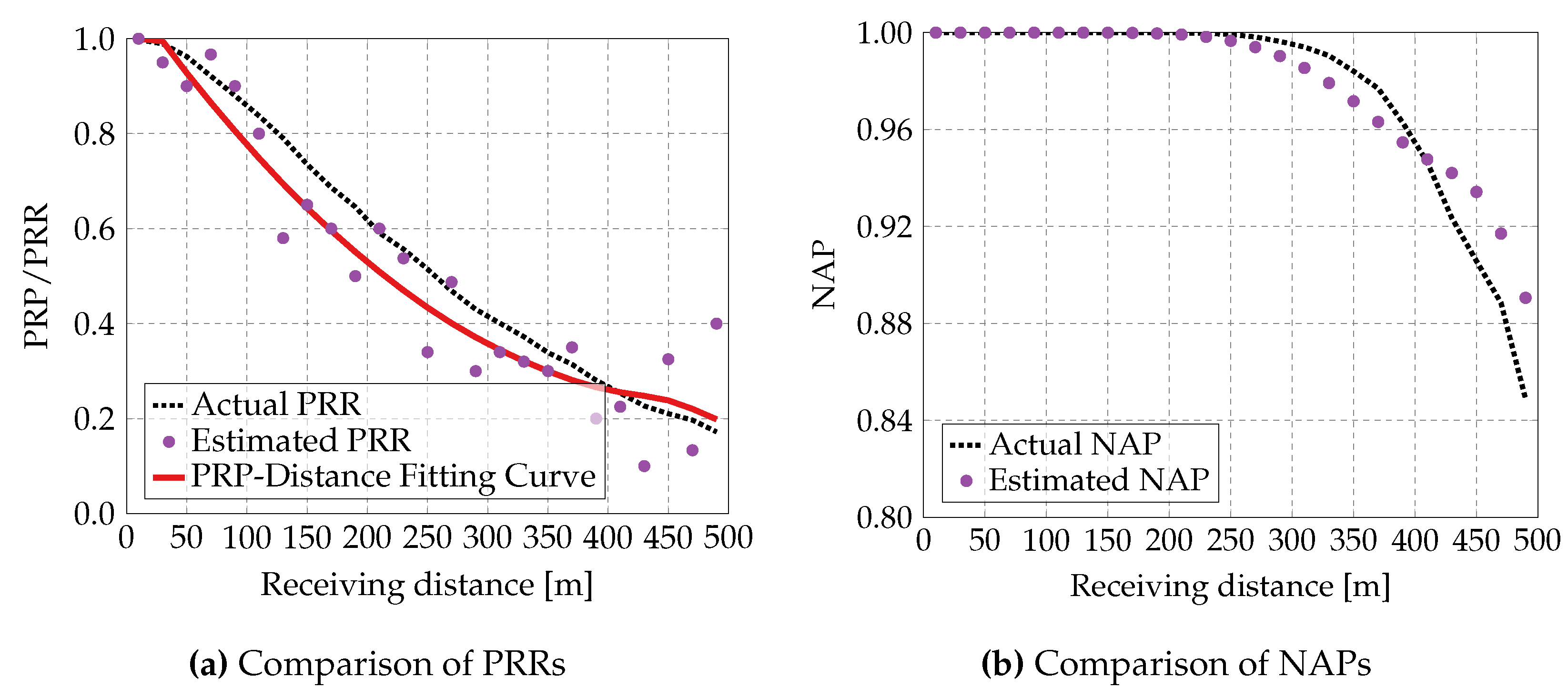
Figure 5.
Comparisons of actual and estimated reliability metrics ( Vehs/m).
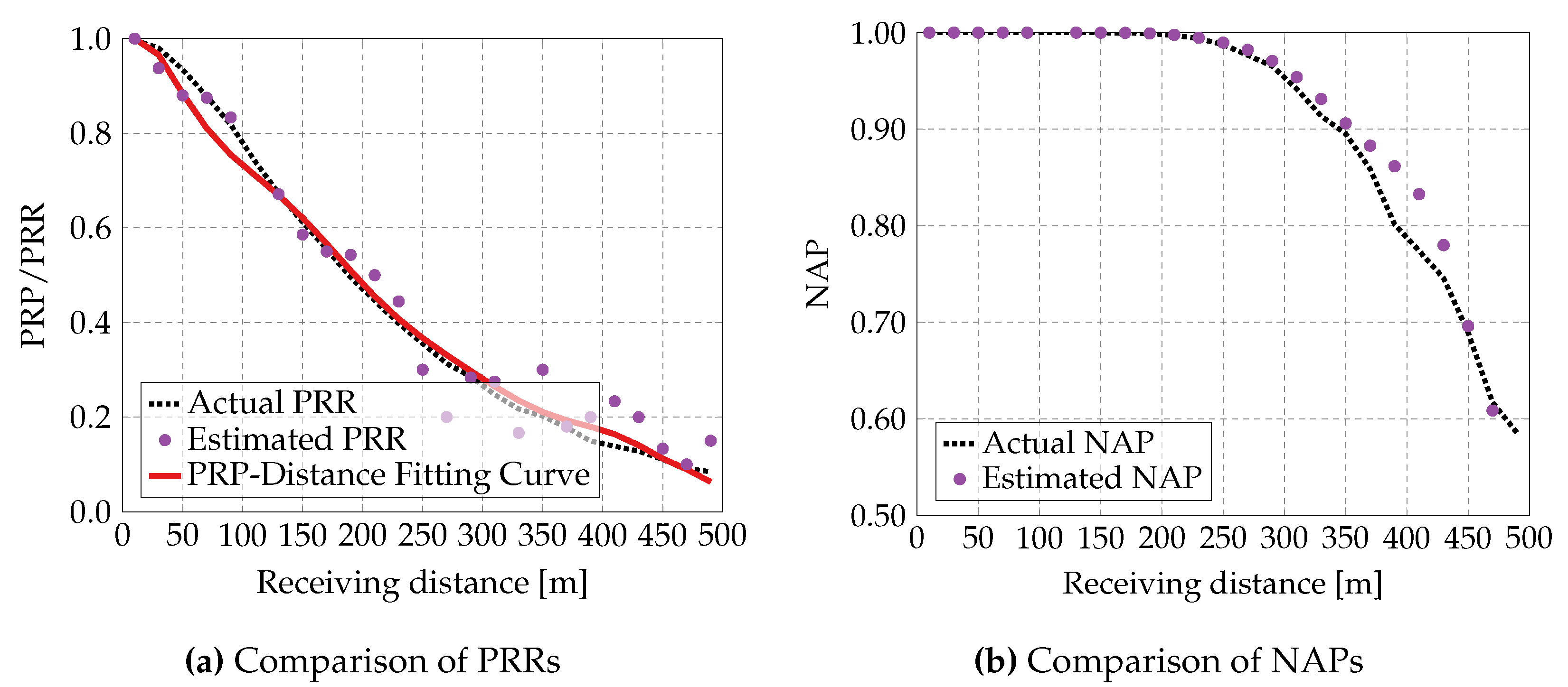
Figure 6.
Comparisons of actual and estimated reliability metrics ( Vehs/m)
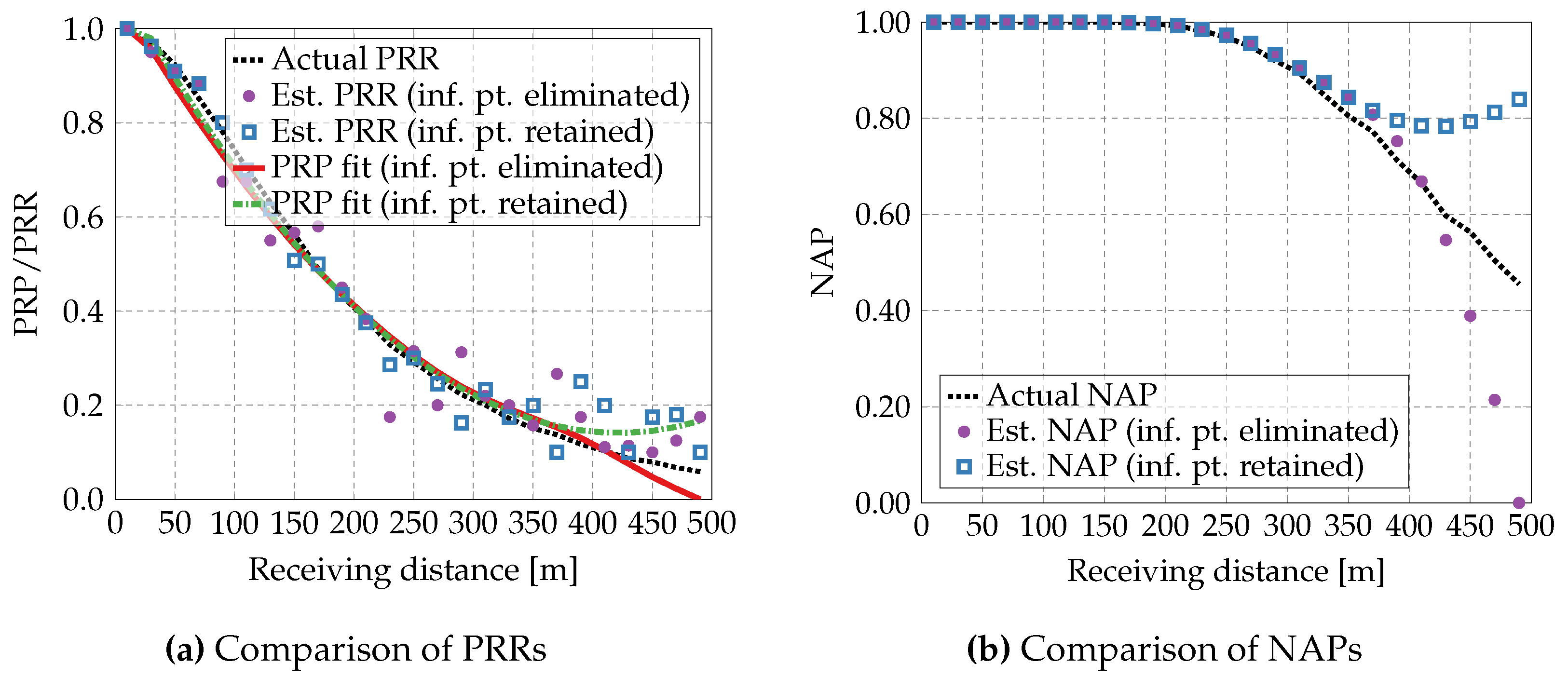
Figure 7.
The number of sensed vehicles and real number of vehicles on road vs. receiving distance ( Vehs/m)
Figure 7.
The number of sensed vehicles and real number of vehicles on road vs. receiving distance ( Vehs/m)
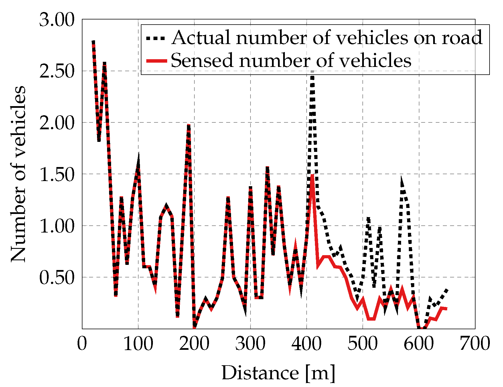
Figure 8.
Comparison between estimated and actual densities
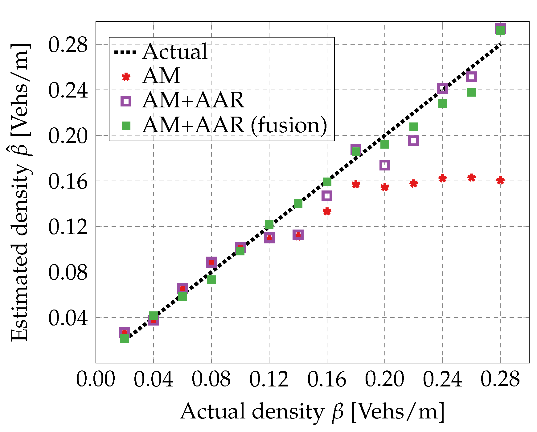
Figure 9.
Effectiveness of the message adjustment based on the proposed vehicle density estimation method
Figure 9.
Effectiveness of the message adjustment based on the proposed vehicle density estimation method
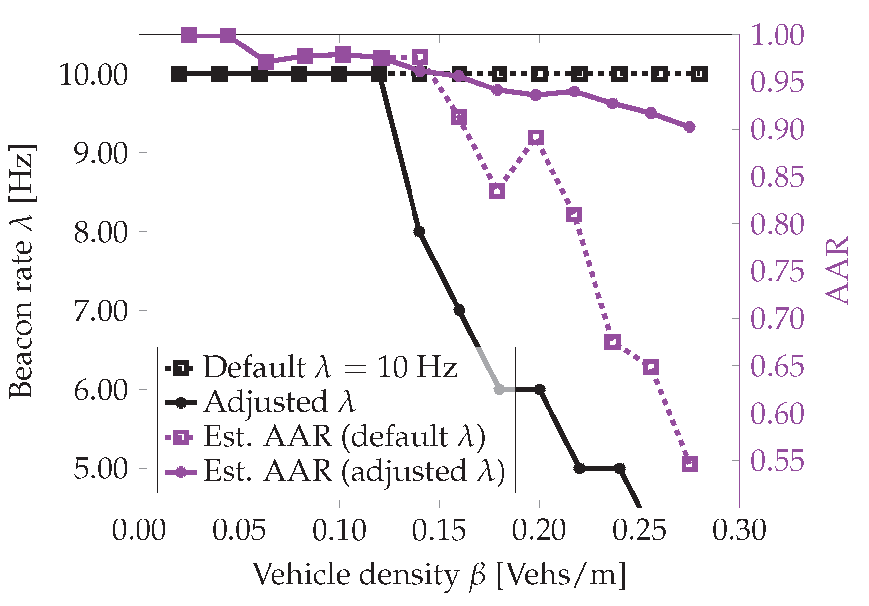

Table 1.
The communication parameters of IEEE 802.11p.
| Parameters | Values |
|---|---|
| Carrier frequency f | 5.9 GHz |
| Channel bandwidth | 10 MHz |
| Carrier sensing threshold | dBm |
| Reference distance | 1 m |
| Noise floor power | dBm |
| Constant | |
| Transmitter gain | 1.0 |
| Receiver gain | 1.0 |
| Modulation and Coding Scheme (MCS) | BPSK, |
| CW W-1 | 15 |
| Path loss exponent | 2 |
| AIFS | 58 µs |
| Packet length PL | 200 bytes |
| Slot time | 13 µs |
| PHY preamble + header | 40 µs |
| MAC header | 272 bits |
| PLCP header | 4 µs |
| Packet generation interval | 0.1 s |
| Fading parameter m, if | 3 |
| Fading parameter m, if | 1.5 |
| Fading parameter m, if | 1 |
Table 2.
The comparison of the accuracy of the estimated vehicle density.
| Actual vehicle density [Vehs/m] | 0.16 | 0.18 | 0.20 | 0.22 | 0.24 | 0.26 | 0.28 |
|---|---|---|---|---|---|---|---|
| Vehicle speed [m/s] | 21.7 | 19.6 | 17.6 | 15.5 | 13.5 | 11.4 | 9.4 |
| Accuracy of AM-based density estimation, Eq. (14) | 0.84 | 0.87 | 0.77 | 0.72 | 0.68 | 0.63 | 0.58 |
| Accuracy of AM-AAR-based density estimation, Eq. (15) | 0.92 | 0.95 | 0.89 | 0.89 | 0.99 | 0.97 | 0.95 |
Disclaimer/Publisher’s Note: The statements, opinions and data contained in all publications are solely those of the individual author(s) and contributor(s) and not of MDPI and/or the editor(s). MDPI and/or the editor(s) disclaim responsibility for any injury to people or property resulting from any ideas, methods, instructions or products referred to in the content. |
© 2025 by the authors. Licensee MDPI, Basel, Switzerland. This article is an open access article distributed under the terms and conditions of the Creative Commons Attribution (CC BY) license (http://creativecommons.org/licenses/by/4.0/).
Copyright: This open access article is published under a Creative Commons CC BY 4.0 license, which permit the free download, distribution, and reuse, provided that the author and preprint are cited in any reuse.


