
Submitted:
20 August 2025
Posted:
28 August 2025
You are already at the latest version
Abstract
This research detailed a hydrochemical investigation and spatial variability examination of the groundwater quality of five principal sites in Kano Region, Nigeria, namely Hotoro, Kano Municipal, Kumbotso, Kofar Fada, and Gezawa, with a total of Fifty-one (51) water samples collected. Physical, chemical and biological parameters assessed in the water samples were Electrical Conductivity, Hardness, pH, Total Dissolved Solids (TDS), Temperature, Turbidity, Dissolved Oxygen (DO2), major cations (Na+, K+, Mg2+, Ca2+) and trace metals (Cr, As, Fe, Zn, Cu, Ni, Pb, Cd). The data demonstrate a high level of spatial heterogeneity that can be considered when examining not only natural geological structures but also anthropogenic factors, particularly urbanized and peri-urban districts of Kano and certain parts of the surroundings, where increased Conductivity, TDS, Hardness, and several ion concentrations were observed. The pH was usually in a slightly acidic to slightly alkaline range, with poor levels of Dissolved Oxygen indicating a possible impact of organic contaminants or the eutrophication phenomenon. Two multivariate visualizations (Boxplots, Scatter plots) and multiple correlation matrices, PCA, and Piper diagrams help clarify the complicated correlation of the constituents of water quality. The Piper diagram revealed unique hydrochemical facies, primarily Sodium-Chloride and Calcium-Magnesium Bicarbonate, which combined the natural geochemistry of sediments with urban anthropogenic effects. The concentrations of Trace metals were generally low with little acute risk proclaimed, but localized areas of potential concern were indicated by periodic increases of Iron and Zinc. The inter-area differences were strongly indicated by statistical testing, which pointed to the need for specific water resource management approaches and pollution control strategies. In general, the combination of spatially addressed hydrochemical observations with the information on spatial data and its analysis presents the opportunity for a crucial contribution to sustainable monitoring of water quality and environmental management in the Kano area, and contributes to rational decisions to preserve the health of the general population and aquatic ecosystems.
Keywords:
hydrochemical characterization
; spatial variability
; groundwater quality
; anthropogenic influences
; and multivariate analysis
Highlights
- Multi-parameter analysis of groundwater quality was carried out in detail in five selected locations in Kano, showing considerable disparities in the physical, chemical, and biological water quality indicators.
- The results of the study showed that a significant spatial heterogeneity was pronounced due to natural geological provisions and human activities, especially urbanization, where more mineralization and levels of existing pollutants were in Hotoro and some areas within Kumbotso.
- Piper plot and multivariate analyses revealed two different types of water, mainly linked to Sodium-Chloride and Calcium-Magnesium Bicarbonate facies, which showed that there was a combination of natural geochemical processes and contamination sources.
- Statistical and geostatistical results underline the necessity of the localized degree of water quality monitoring and pollution control to secure individual health and aquatic fauna in the Kano area.
Introduction
What unexplored information about water quality and contamination is contained in the peaks and patterns of ion and trace metal chromatograms of such different locations at Hotoro, Kano Municipal, and Garun Mallam as we can interpret the geochemical fingerprints and footprints of groundwater contamination of groundwater’s in critical areas of Nigeria through the deciphering of the complex peaks of chromatogram plots to achieve more intelligent environment management and preservation of resources."
The research by Ifie-emi 2025) used remote sensing and GIS to analyze spatial patterns of Electrical Conductivity (EC), Total Dissolved Solids (TDS), and pH in the Gurara Reservoir, Nigeria. The study found that pollution loads increased downstream in the reservoir, with EC and TDS closely related and generally higher in those areas. The upstream regions showed higher pH values, likely due to geological weathering processes. By mapping these parameters using GIS techniques, the research highlighted the impacts of land-use changes and human activities on water quality. The study confirms the critical role of GIS in providing visual insights for ongoing monitoring and effective management of reservoir water resources, underpinning the need for strategic protection plans to safeguard the reservoir's water quality for current and future use. This has led to disproportionate ecological degradation and increased health risks due to the absence of regular risk assessments, highlighting the urgent need for systematic, ongoing monitoring to manage water quality sustainably. The 2025 study published in Frontiers in Water integrates GIS with hydrochemical analyses to model and visualize groundwater quality, focusing on key parameters such as electrical conductivity (EC) and total dissolved solids (TDS). The research demonstrates spatial variations in TDS ranging from 2,304 to 8,832 mg/L and EC from 3,600 to 13,800 µS/cm, influenced strongly by regional geology and land use practices. The findings indicate generally poor groundwater quality for both irrigation and drinking purposes due to contamination from agricultural runoff, industrial discharges, and overexploitation. There is a need for comprehensive, continuous, and integrated GIS-based monitoring systems to accurately capture spatial and temporal variations, assess contamination sources, and inform sustainable groundwater management and policy decisions effectively. (Hanaa et al., 2025)
(Jalal and Mahsas 2025) A study of selected wells in the Taleghan region, Iran, used geospatial analysis to evaluate groundwater quality indicators, primarily electrical conductivity (EC) and total dissolved solids (TDS). The research identified significant correlations between the geological characteristics of the region and variations in water chemistry, indicating that the local geology strongly influences groundwater quality. These findings emphasize the importance of incorporating geological factors in groundwater management and protection strategies to ensure safe and sustainable water resources, but a limited multi-seasonal and spatially comprehensive groundwater quality data in the Taleghan region. There is a need for ongoing monitoring incorporating diverse hydrochemical parameters and microbial risks to better understand temporal variations and human impacts on groundwater quality. The 2025 study on groundwater quality in polluted hotspots of Nigeria employs geospatial analysis to map key parameters such as electrical conductivity and total dissolved solids. A significant spatial variation driven by anthropogenic activities and geological factors, demonstrating how urbanization and industrial pollution degrade groundwater quality. The study underscores the effectiveness of GIS-based visualization tools in identifying contamination patterns and supporting targeted interventions for groundwater management in urban and peri-urban environments (Oseke, 2025). There is a need for enhanced GIS-integrated monitoring frameworks to capture dynamic pollution sources, improve contamination source attribution, and inform sustainable urban groundwater management strategies (Emoyan et al., 2008). The study on groundwater quality assessment in polluted hotspots of Tamil Nadu, India, integrates geospatial and statistical approaches to evaluate key water quality parameters. The research identifies significant spatial variability in contamination levels influenced by industrial activities, agricultural runoff, and geological factors. Using GIS mapping and multivariate statistical analysis, the study effectively highlights areas with elevated electrical conductivity and total dissolved solids, underscoring the combined impact of anthropogenic pressures and natural geology on groundwater quality. The findings provide crucial insights for targeted groundwater management and pollution mitigation strategies in the region. Limited integration of high-resolution temporal data and comprehensive multi-parameter monitoring constrains the understanding of groundwater quality dynamics in Tamil Nadu. Enhanced GIS-based, long-term studies are needed to capture seasonal variations and pinpoint pollution sources for effective groundwater management and policy formulation. (Barath et al., 2025). The study employed ten vertical electrical soundings (VES) to determine the bedrock depth in the Liji area of Gombe State using geophysical techniques. The majority of geo-electric layers detected by the WINRESIST program displayed three or four layers. Basement rocks with an unlimited thickness were discovered at depths between 5.7 and 24.0 meters. The Western, Northwestern, and Eastern parts displayed significant resistivity values, and the A-curve was widely present. (Garba et al., 2024). The deteriorating water quality of the Baitarani River in Odisha, India, highlights pollution from both urban, agricultural, and industrial sectors. He categorizes contamination degrees, spotlights hotspots, and forecasts the water quality most accurately, which calls for actionable interventions, community local actions, and policy changes to have sustainable management of rivers (Abhijeet, 2025).
Research on Ain Sefra, located in South West Algeria, which is vital amidst the arid conditions, especially in welling and ground products. They are determined using multivariate stats, water quality indices, and geochemical modeling, where the samples can be divided into four hydrochemical groups, which are mostly fit to be used in drinking and agricultural purposes. The prominent processes are the dissolution of minerals and pollution. Results reiterate the need to incorporate management as well as constant observation and GIS observation to assure sustainable use of groundwater under pressures of climate and population (Bellal et al., 2024). In an experiment conducted in Lawspet, India, it was found through multivariate analysis that man-made activities such as waste dumping and waste reuse have a drastic negative impact on the quality of groundwater. Meaningful parameters like EC, TDS, and Cl- exhibit spatial variation, and the statistical significance of the variance throughout the sites was established; thus, there is a pertinent demand for management and monitoring of sustainable waste strategies (Suresh et al., 2017). The analysis was conducted to analyze the borehole water quality in Effurun, Nigeria, with a focus on water contamination by agricultural and industrial activities, including the high concentration of nitrate, sulfate, and lead. Through hydrochemical, statistical, and geospatial techniques, it targets contamination hotspots and underlines the necessity of continuous monitoring, mitigation activities, and community participation in the management of healthy drinking water and sustained management of groundwater (Odunnayo et al., 2025). The quality of groundwater is evaluated in Uttarakhand, India, and groundwater is found to be an alkaline, hard water of the Ca-Mg-HCO3 weathered nature that is affected by natural and anthropogenic factors. Salinity and hardness are the factors of concern, being high, mostly meeting standards. Statistical analysis provides sources of contamination and the fact that areas are fit to carry out irrigation. They should sustainably manage and monitor it regularly to preserve this important Himalayan water resource (Nayak et al., 2022). Shaheed Benazirabad is the city of the Indus River with a population of 1.613 million people and an arid/ semi-arid climate. The water samples taken at a depth of 40m are dominated by Calcium chloride, and it was observed that this was determined by water-rock interaction. Qualities of groundwater depend much on soil types and climatic modulations, and spatial variations occur based on land use patterns, plants, and urbanization, being an imperative area of water management. Groundwater quality in North Bahri City, Sudan, focusing on the Nubian sandstone aquifer using hydrochemical and multivariate analyses. Results show Ca-Mg-HCO3 water types influenced by geology and human activities like agriculture and septic contamination. About 75% of samples suit irrigation, though salinity issues exist, highlighting the need for integrated chemical and statistical monitoring for sustainable groundwater management (Musaab et al., 2022). The population assessment of groundwater in Sharsa Upazila in Bangladesh indicates the contamination of groundwater due to agricultural and waste enterprises, where some places are at a health risk. It depicts variable quality using GIS, indices, and multivariate analyses that necessitate sustainable management, control of pollution, and remediation to guarantee safe drinking water and agricultural applications against environmental pressures (Ghoto et al., 2025). The concentrations of dissolved Ca++, Fe++, and Cl- in water samples provide the basis for the Water Quality Index (WQI) values. Except for Ghuzukwi, hand-dug wells are of poor and very poor quality, whereas borehole sources have good WQI ranges. Hand-dug wells should be properly treated, including chlorine treatment and a safe distance from pit latrines. Water quality can be enhanced at the household level using low-cost interventions. (Garba, et al., 2014). In the Sharsha Upazila, Jashore District, Bangladesh, 69% samples were above the standard of NH4+, as well as 100% of Ca2+. The Water Quality Index (WQI) showed good quality in most of the water to be used for drinking. Contaminants were spatially distributed by using GIS mapping. According to PCA, large anthropogenic and geogenic impacts on the quality of water were identified. Groundwater is, in most cases, acceptable to use in irrigation, though there are grounds that pose health hazards because there are excessive levels of the ions (Mohammed et al., 2024).
Aims and Objective:
The primary purpose of this research is to justify and define the spatial nature as well as the multi-parametric processes of groundwater quality in a number of Nigerian regions, such as Hotoro, Kano Municipal, Kumbotso, Kofar Fada, and Gezawa. It seeks to determine and analyze the natural hydro-geochemical processes in these places and the influence of man that interferes with the water chemistry. In attaining this, different statistical, graphical, and analytical tools, e.g., boxplots, scatter plots, violin plots, chromatograms, correlation, principal component analysis (PCA), and calibration curves, were utilized to give an accurate overview of the quality of water. Its outputs are supposed to be used in specific decision-making in the management of water resources and the environment, to enable them to ensure that management is sustainable and efficient based on solid analysis of data obtained on multiple parameters of water quality. The spatial distribution of water quality in the regions under examination is characterized by high variances leading to spatial heterogeneity, which is caused not only by natural, geological impacts but also by the level of anthropogenic impact. Some of these important physicochemical parameters, which include Conductivity, Total Dissolved Solids (TDS), Hardness, and pH, have significant disparities across locations due to differences in mineralization level and pollution. Data visualization of multivariate controls and statistical interpolations shows high correlations between major ions and trace metals and may assist in locating geochemical links, sources of contamination, and particular regions of water quality importance. Combining Chromatograms, Scatter plots, correlation Heatmaps, and Principal Component Analysis (PCA), it is possible to reduce the complex contamination compositions to transparent and understandable patterns, helping to diagnose the contamination, the influence of natural hydro-geochemical processes, and general water quality situations.
Materials and Methods
Water samples were systematically gathered through different locations in the Kano region of Northern Nigeria, which is geographically restricted together with the latitudinal corner areas of 8° 02ʺ and 8° 59ʺ N and longitudinal axis range 11° 00ʺ and 12° 14ʺ E. The sampling locations have been chosen as Hotoro, Kano Municipal, Kumbotso, Kofar Fada, Gezawa, and Garun Mallam, among others, which cover different degrees of urbanization, geological environment, and plausible pollution sources. The spatial segregation of sample points and analysis of sampling point data facilitated comparative studies to determine how geomaterial, anthropogenic activities, and land use affect changes to water quality. Standard environmental procedures were considered in the sampling collection procedures to be representative and reduce contamination. Sterile bottles have been applied, and the sampling depth has been followed effectively and allowing sample integrity to be conserved during transport of samples. Temperature, pH, electrical conductivity, turbidity, and dissolved oxygen (DO2) measurements were taken in the field with calibrated portable probes to obtain as precise as possible in situ conditions. Parameters of water quality being monitored were physical, chemical, and biological Markers. Physical parameters were temperature (degrees Celsius), turbidity (Nephelometric Turbidity Units), and dissolved oxygen (mg/L) measured with an electrochemical or optical probe. Chemical parameters included electrical conductivity (mS/cm) to measure ionic strength, total dissolved solids (TDS, mg/L) using a gravimetric method after filtration, pH, which indicated a measure of acidity or alkalinity, and hardness as an indication of concentrations of calcium and magnesium. The measurement of major ions sodium (Na+), Potassium (K+), Magnesium (Mg2+), Calcium (Ca2+), Chloride (Cl+), Sulfate (SO42-), Nitrate (NO3-), and Bicarbonate (HCO3-) and the measurement of trace Metals chromium (Cr), Arsenic (As), Iron (Fe), zinc (Zn), and copper (Cu), Nickel (Ni), Lead (Pb) and cadmium (Cd).
Quality assurance was maintained through the use of standard calibration curves based on certified reference standards across broad concentration ranges, ensuring linearity and accuracy. Precision was validated by multiple replicates and quality control samples, minimizing analytical errors and confirming consistency. Routine blanks were analyzed to check for contamination or instrument drift. The quality assurance was carried out in terms of using the standard calibration curves according to the certified reference standards in the case relating to the wide concentration ranges, and was in terms of linearity and accurate results. Multiple replicates and quality control samples validated precision and reduced analytical errors, and assured consistency. Blank runs as a routine were investigated to see whether there is any contamination or variation in the instrument. Descriptive statistics and comparative tests like t-tests and confidence interval estimates were used in the analysis to determine significant spatial variation of sampling zones. Statistical methods such as correlation matrices, principal component analysis (PCA), and Piper diagrams, provided the basis of comprehension of complex ionic correspondences and geochemical sources, as well as facies hydrochemical. Kriging approaches were used in geostatistical approaches to spatially interpolate and map variability in the water quality parameters. Visual representations, such as box plot, scatter plot, violin plot, pair-wise correlation, and chromatogram plot, delivered multidimensional information on the water chemistry trends, as well as allowed locating the hot areas of contamination. The composite interpretive structure incorporated physical/chemical and biological data to deliver a strong evaluation of water quality and ecosystem health throughout the area. Correlation and geographic analysis separated the naturally occurring influences of geochemical impacts and the man-made pollution. Positive correlations among important cations at all points showed that mineral dissolution and interaction with water occurred, and occasional peak values of trace metals were evidence that contamination occurred in localized areas. Multivariate analysis was able to condense complex data sets into patterns that can be recognized to inform specific environmental management, monitoring, and remediation actions. Such methodological design guaranteed accurate and dependable measurement of water quality in spatially heterogeneous urban–peri–urban locations in Kano, as well as data-driven decision-making in the management of water resources and ecological integrity conservation.
Results
The dataset provides a precise record of water quality as measured at various points along the water sampling sites in the Kano region of Nigeria, with all the data points centered at latitudes between 8° 02ʹ and 8° 59ʹ and longitudes between 11° 00ʹ and 12° 14ʹ. Parameters that are monitored are electrical conductivity, hardness, pH, total dissolved solids (TDS), temperature, turbidity, and dissolved oxygen (DO2). All these parameters indicate physical, chemical, and biological factors of water quality. Spatial agglomeration of sample points allows to conduct a comparative analysis of differences in the quality of water based on the geology of the area, urbanization, and sources of pollution.
Electrical conductivity of the water, which measures the water's capacity to conduct current as a result of the ionic content, also records a wide range, with a low of around 176.2 µS/cm up to very high records above 2400 µS/cm at certain Hotoro and Ring Road, among others. Such high conductivity values will be associated with high TDS and hardness values, indicating mineral-rich or possibly polluted water that may most likely be caused by natural mineralization of groundwater or manmade activities. The majority of pH cases are within a general range of slightly acidic to slightly alkaline (~5.6 and ~8.7, respectively) and therefore acceptable as drinking water, although some cases are borderline and may be considered acidic and contribute to corrosiveness and leaching of metals in pipes. Moderate changes are recorded in the turbidity values, varying between 8 and 19 NTU, the meaning of which is that the suspended solids are changing, thus affecting the water clarity and harboring pathogens, resulting in difficulties in providing water treatment and supporting aquatic organisms.
Temperature fluctuates minimally between 29 and 33o °C, characteristic of a tropical climate, thus having the inverse effect on the solubility of dissolved oxygen. Dissolved oxygen varies between approximately 2.3 mg/L and 6.9 mg/L, but the lower Dissolved oxygen is often observed where there is a high conductivity level and TDS, which may indicate organic contamination or eutrophication of the water and the use up of the oxygen. The increased turbidity areas are usually accompanied by low DO, meaning biologically active waters or heavy sediment characterizing waters. In general, the data indicate a lot of heterogeneity in the case of water quality, which can be attributed to a complicated interplay between geology, land use, and humanity. Constant monitoring and localised management of these water sources in these peri-urban and urban areas is important to ensure the quality and the sustenance of water resources and the aquatic ecosystem.
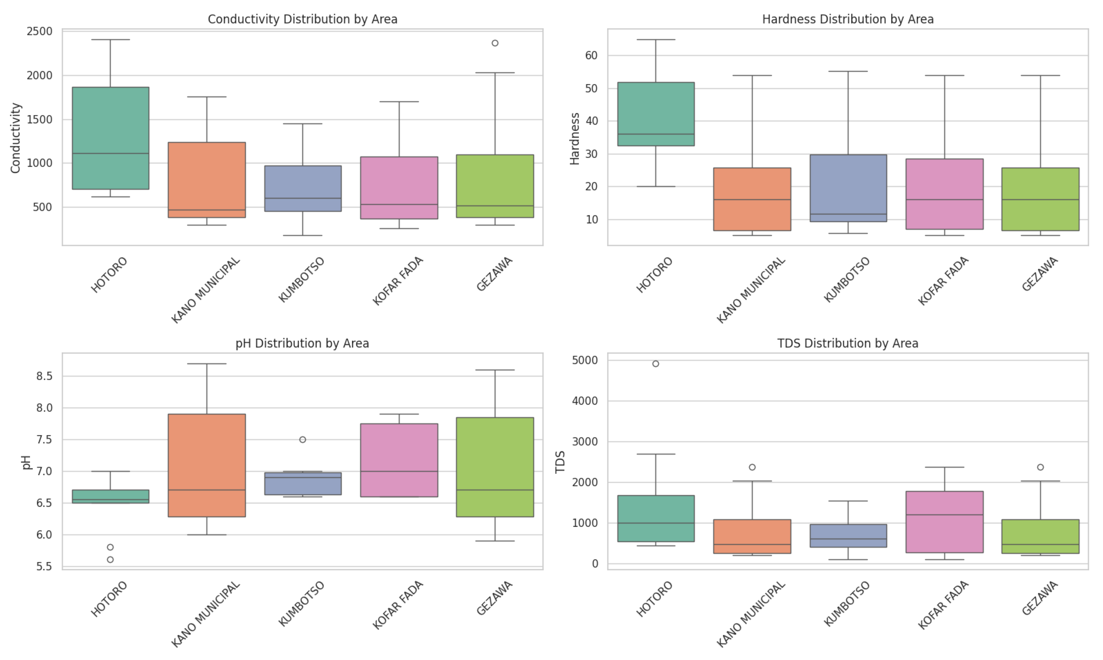
The water quality measurements in the areas of Hotoro, Kano Municipal, Kumbotso, Kofar Fada, and Gezawa show that there exist certain spatial and parameter-specific changes that can only be attributed to the possible presence of both natural and anthropogenic factors affecting the water quality. Boxplots indicate a disparity in vital characteristics like conductivity, hardness, pH, and total dissolved solids (TDS) among these localities, with the HOTORO zone and some KUMBOTSO locations featuring substantially higher values of conductivity and TDS, probably due to the volume of minerals or pollutants related to the climate of urbanization or geographical conditions. It can be seen in the scatter plot of pH against dissolved oxygen (DO2) that, as a rule, more neutral to slightly alkaline waters have higher concentrations of oxygen which is essential to aquatic life, whereas lower pH values, are associated with lower DO which might have signs of local contamination and may be a cause of local depletion of oxygen. (Figure 1).

Table 1.
Showing all the 51 Locations with their Longitudes, Latitudes, Conductivity, Hardness, pH, TDS, Temperature, Turbidity, and DO2.
Table 1.
Showing all the 51 Locations with their Longitudes, Latitudes, Conductivity, Hardness, pH, TDS, Temperature, Turbidity, and DO2.
| S/No | Name | Long. | Lat. | Conductivity | Hardness | pH | TDS | Temperature | Turbidity | DO2 |
|---|---|---|---|---|---|---|---|---|---|---|
|
1 |
Sabon bakin zuwo Hotoro GRA | 11.00 | 8.20 | 616.5 | 54 | 7.0 | 525.7 | 32.6 | 12 | 5.6 |
| No. 6 Hotoro Avenue | 11.24 | 8.16 | 929.6 | 34 | 6.7 | 640.8 | 29.4 | 11 | 5.3 | |
| Hotoro | 11.33 | 8.06 | 2410 | 32 | 6.5 | 1673 | 30.5 | 16 | 3.4 | |
| No. 1 Sabo Bakin Zuwo Road. | 11.11 | 8.56 | 1847 | 20 | 6.5 | 1272 | 31.7 | 15 | 3.2 | |
| No. 13 Sabo Bakin Zuwo Road | 11.18 | 8.43 | 2410 | 36 | 6.7 | 1673 | 29.9 | 13 | 2.3 | |
| Tarauni | 11.01 | 8.12 | 651.3 | 36 | 6.8 | 450.4 | 31.1 | 10 | 5.3 | |
| Eastern Bypass Hotoro Kano | 11.49 | 8.71 | 1289 | 65 | 6.6 | 737.9 | 30.0 | 9 | 3.6 | |
| No. 70 Ring Road Bypass | 113.9 | 8.22 | 1871 | 45 | 5.6 | 2700 | 30.9 | 19 | 2.4 | |
| No. 34 Ring Road Bypass | 11.19 | 8.30 | 702.3 | 62 | 5.8 | 484.3 | 30.8 | 10 | 4.9 | |
| Hotoro Kano | 11.22 | 8.24 | 715 | 31 | 6.5 | 4917 | 29.9 | 9 | 5.3 | |
|
2 |
Kano Municipal 1 | 11.17 | 8.31 | 293.7 | 6 | 6.9 | 202 | 30.0 | 9 | 5.3 |
| Kano Municipal 2 | 11.22 | 8.30 | 371.2 | 16 | 6.1 | 256.1 | 30.9 | 8 | 5.2 | |
| Kano Municipal 3 | 11.46 | 8.31 | 346.0 | 54 | 6.5 | 239.0 | 30.8 | 14 | 5.6 | |
| Kano Municipal 4 | 11.19 | 8.31 | 753.1 | 6 | 7.6 | 520.1 | 29.9 | 12 | 4.9 | |
| Kano Municipal 5 | 11.44 | 8.31 | 415.0 | 8 | 6.2 | 286.4 | 30.0 | 13 | 5.5 | |
| Kano Municipal 6 | 11.29 | 8.31 | 507.7 | 5 | 6.5 | 734.5 | 29.4 | 16 | 5.3 | |
| Kano Municipal 7 | 11.36 | 8.31 | 424.2 | 16 | 6.0 | 424.2 | 30.5 | 9 | 5.7 | |
| Kano Municipal 8 | 11.25 | 8.32 | 1402 | 25 | 8.7 | 2030 | 31.7 | 19 | 3.2 | |
| Kano Municipal 9 | 11.46 | 8.31 | 1757 | 26 | 8.0 | 1211 | 29.9 | 13 | 3.6 | |
| Kano Municipal 10 | 11.48 | 8.32 | 1633 | 35 | 8.5 | 2370 | 29.4 | 16 | 2.6 | |
|
3 |
Kumbotso 1 | 12.05 | 8.54 | 1365 | 34.6 | 6.6 | 1546 | 32.1 | 13 | 5.6 |
| Kumbotso 2 | 12.07 | 8.55 | 377.4 | 54.3 | 6.9 | 514.8 | 30.8 | 16 | 5.2 | |
| Kumbotso 3 | 12.08 | 8.56 | 413.1 | 55.2 | 6.6 | 285.0 | 29.9 | 9 | 4.6 | |
| Kumbotso 4 | 12.09 | 8.57 | 603.1 | 12.6 | 7.0 | 420.8 | 30.0 | 19 | 5.2 | |
| Kumbotso 5 | 12.09 | 8.59 | 1452 | 10.5 | 6.7 | 1001 | 30.9 | 11 | 6.9 | |
| Kumbotso 6 | 12.10 | 8.59 | 176.2 | 15.0 | 7.5 | 115.2 | 30.8 | 13 | 5.6 | |
| Kumbotso 7 | 12.11 | 8.10 | 905.2 | 9.6 | 6.9 | 1308 | 29.9 | 11 | 5.9 | |
| Kumbotso 8 | 12.12 | 8.21 | 610.2 | 6.1 | 7.0 | 884.9 | 30.0 | 16 | 6.3 | |
| Kumbotso 9 | 12.13 | 8.52 | 576.0 | 9.3 | 6.6 | 399.0 | 29.4 | 13 | 5.5 | |
| Kumbotso 10 | 12.14 | 8.03 | 992.5 | 5.8 | 6.9 | 720.5 | 30.8 | 10 | 6.4 | |
|
4 |
Aliko Oil Fueling Station | 11.38 | 8.26 | 323 | 31 | 7.8 | 2030 | 32.1 | 10 | 5.7 |
| HJRBDA Office | 11.38 | 8.27 | 257 | 6 | 7.1 | 1211 | 31.7 | 9 | 3.2 | |
| Kadawa Pri. Health Care | 11.38 | 8.27 | 534 | 16 | 7.0 | 2370 | 29.5 | 9 | 3.6 | |
| Tangala | 11.38 | 8.27 | 1499 | 54 | 7.7 | 1546 | 32.6 | 8 | 2.6 | |
| Kofar Fada Jummat Mosque | 11.38 | 8.24 | 1704 | 6 | 7.9 | 514.8 | 30.3 | 14 | 5.6 | |
| Makara Huta Borehole | 11.38 | 8.27 | 1312 | 8 | 7.9 | 225.0 | 32.3 | 12 | 5.2 | |
| Rijiyar Isha’u | 11.39 | 8.25 | 727 | 5 | 6.6 | 320.8 | 29.0 | 13 | 4.6 | |
| Rijiyar Gidan Ganji | 11.38 | 8.27 | 831 | 16 | 6.6 | 101 | 29.6 | 16 | 5.2 | |
| Maza Waje Borehole | 11.39 | 8.24 | 367 | 25 | 6.6 | 105.2 | 30.0 | 9 | 6.9 | |
| Ali Yage Borehole | 11.38 | 8.26 | 367 | 26 | 6.7 | 1208 | 31.0 | 19 | 5.6 | |
| Rijiyar Gidan Mallam Kabiru | 11.38 | 8.24 | 444 | 35 | 6.6 | 2043 | 32.6 | 13 | 5.7 | |
|
5 |
Babawa 1 | 12.00 | 8.41 | 293.7 | 6 | 6.9 | 202 | 29.4 | 9 | 5.3 |
| Babawa 2 | 12.00 | 8.51 | 371.2 | 16 | 6.1 | 256.1 | 32.1 | 8 | 5.2 | |
| Kawaji | 12.00 | 8.52 | 346.0 | 54 | 6.5 | 239.0 | 30.8 | 14 | 5.6 | |
| Babawa 3 | 12.00 | 8.12 | 753.1 | 6 | 7.7 | 520.1 | 29.9 | 12 | 4.9 | |
| Kano, Gumel Road | 12.00 | 8.02 | 415.0 | 8 | 6.2 | 286.4 | 30.0 | 13 | 5.5 | |
| Babawa 4 | 12.00 | 8.33 | 507.7 | 5 | 6.5 | 734.5 | 30.9 | 16 | 5.3 | |
| Gezawa 1 | 12.00 | 8.22 | 524.2 | 16 | 5.9 | 424.2 | 30.8 | 9 | 5.7 | |
| Gezawa 2 | 12.00 | 8.02 | 2030 | 25 | 8.6 | 2030 | 29.9 | 19 | 3.2 | |
| Babawa 7 | 12.00 | 8.51 | 1211 | 26 | 7.9 | 1211 | 30.0 | 13 | 3.6 | |
| Kawaji 2 | 12.01 | 8.10 | 2370 | 35 | 8.5 | 2370 | 29.4 | 16 | 2.6 |
Figure 1.
Distribution patterns of Conductivity, Hardness, pH, TDS, Temperature, Turbidity, and DO2 in the study area.
Figure 1.
Distribution patterns of Conductivity, Hardness, pH, TDS, Temperature, Turbidity, and DO2 in the study area.
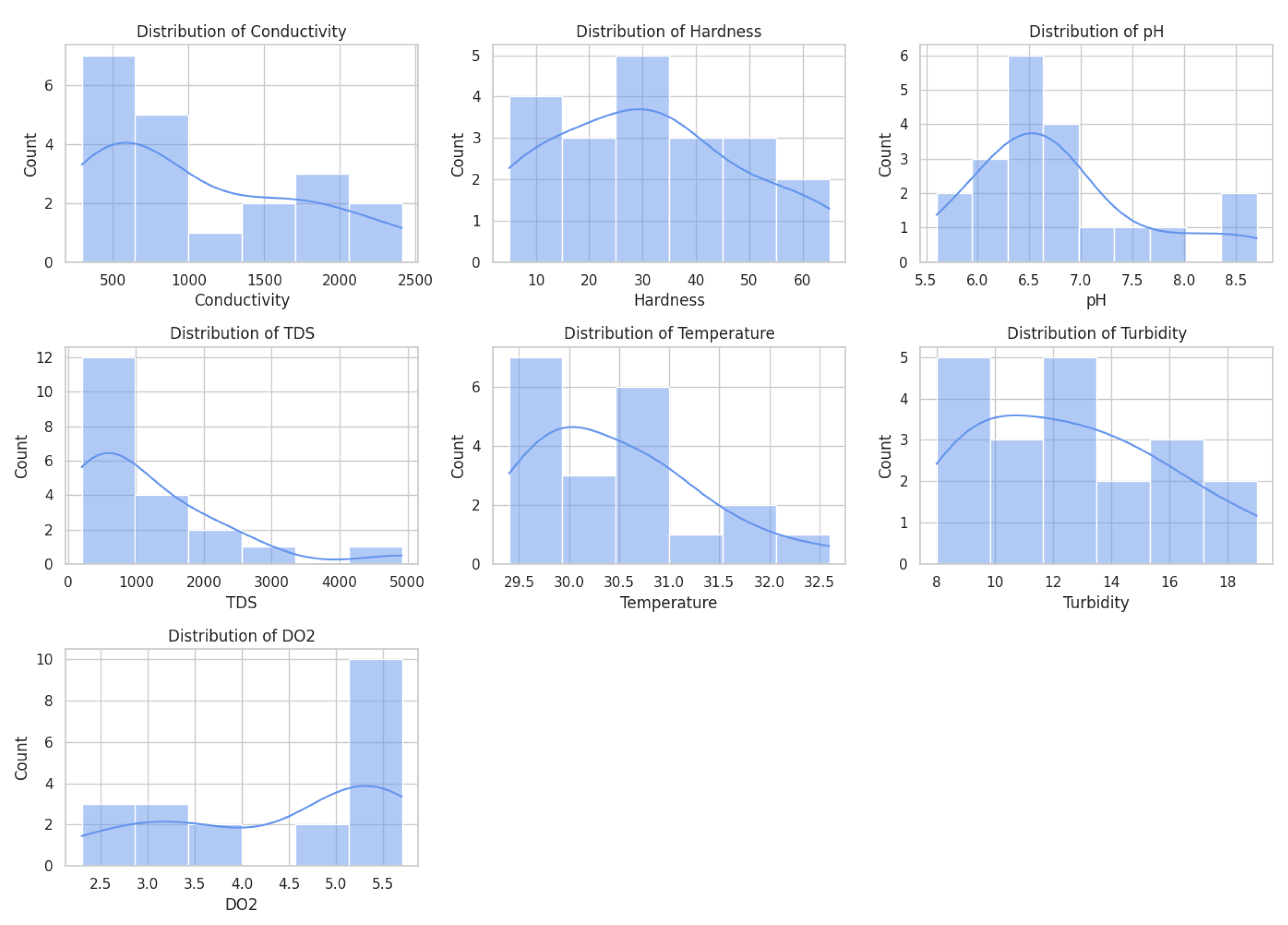
Figure 2.
Violin Plots of Conductivity Hardness, pH, and TDS distribution in the study area.
Where the violin plots indicate scattered patterns of suspended solids across spatial locations, the plots of turbidity demonstrate greater dispersion of turbidity in KOFAR FADA, which could imply natural sediment accretion or urban wastes. The pairplot also shows the correlation, like a positive relationship of conductivity to TDS, which confirms that in these water sources, an increased presence of dissolved solids is also accompanied by increased ion content. The various visualization tools, boxplots, scatter plots, violins, and pairwise relationships allow them to come up with a unified picture of how the various parameters of water quality interact spatially and physico-chemically in different locations, thus helping them to be able to monitor and manage the environment in a more targeted fashion. In general, the nature of the plotted data indicates a hydrochemical landscape of great complexity with localised hotspots of several parameters of mineralization, acidity, and biological oxygen demand, indicative of a spatial heterogeneity in land use, pollution sources, and geology. This comprehensive science visualization highlights the importance of multi-parameter evaluation, which is necessary to accurately represent water quality statuses and provide informed planning decisions for sustainable management of water resources in these Nigerian regions. It is consistent with standard approaches to analysis of water quality data, in which a combination of physical, chemical, and biological indicators produces strong information on the health of an ecosystem and the effect humans have on it.
t-test Plots Analysis
The plots show that there is a difference in the water quality between HOTORO, KANO MUNICIPAL, KUMBOTSO, KOFAR FADA, and GEZAWA. HOTORO and some areas of KUMBOTSO exhibit considerably high conductivity and TDS, and hardness, which is shown to have high mineralization or pollution, possibly through urban factors. Overall, pH values mainly remain close to neutral, though with some variation that manifests in changing water chemistry and impacts on aquatic health. The amount of dissolved oxygen tends to decline with conductivity and turbidity, which indicates that at maximum sites where the pollutant load is high, oxygen deficiency is experienced, which affects biological feasibility. Statistical testing reveals noticeable inter-area variability of major parameters, which is attributed to spatial heterogeneity under the complex impact of geological and anthropogenic activities, requiring the introduction of special water quality management as well.
Figure 3.
showing (a) Boxplot and Pairwise t-test for Conductivity, (b) Boxplot and Pairwise t-test for Conductivity, (C) Boxplot and Pairwise t-test for pH, (d) Boxplot and Pairwise t-test TDS, € Boxplot and Pairwise t-test for Temperature, (f) Boxplot and Pairwise t-test for Turbidity and (G) Boxplot and Pairwise t-test for DO2.
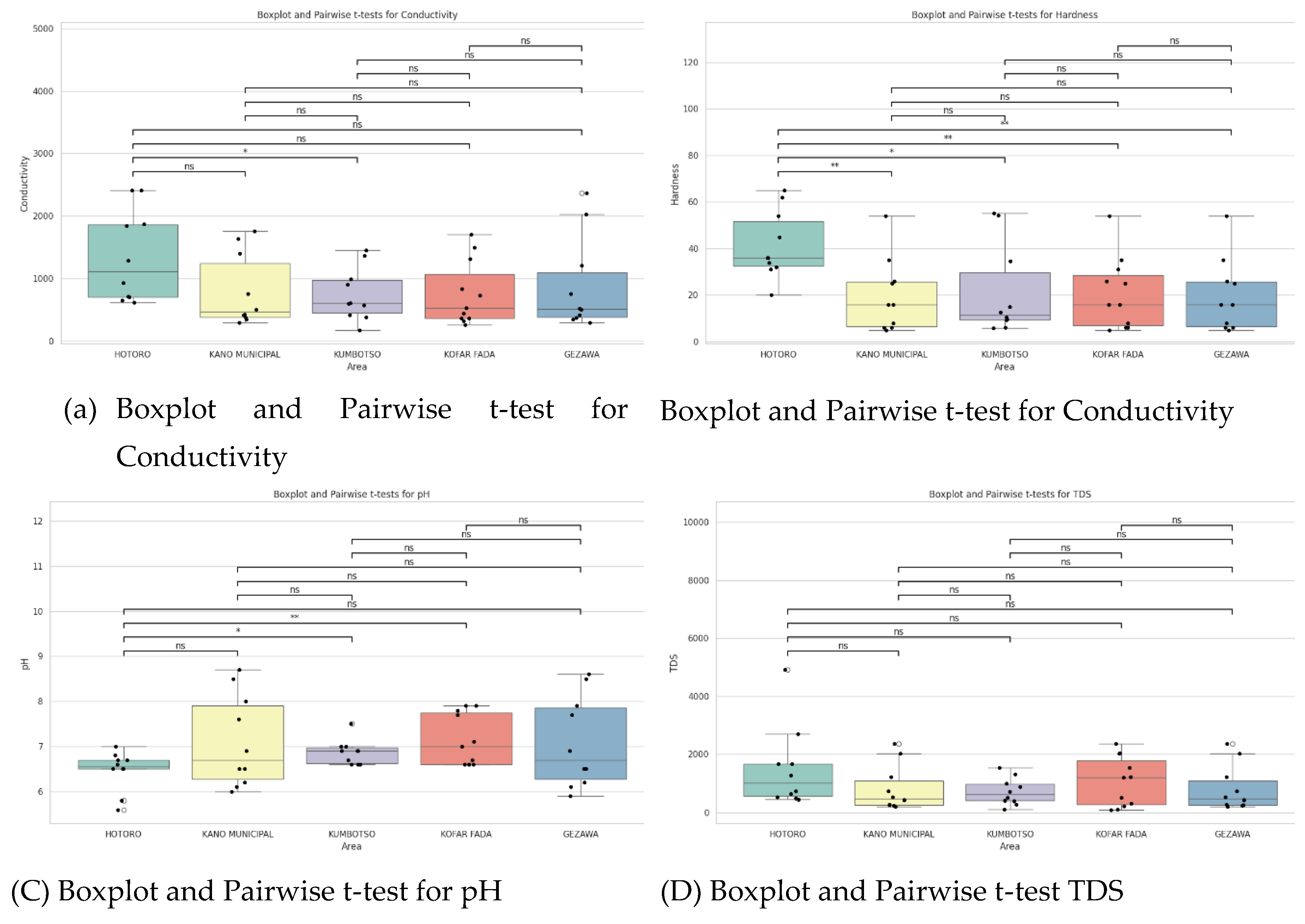
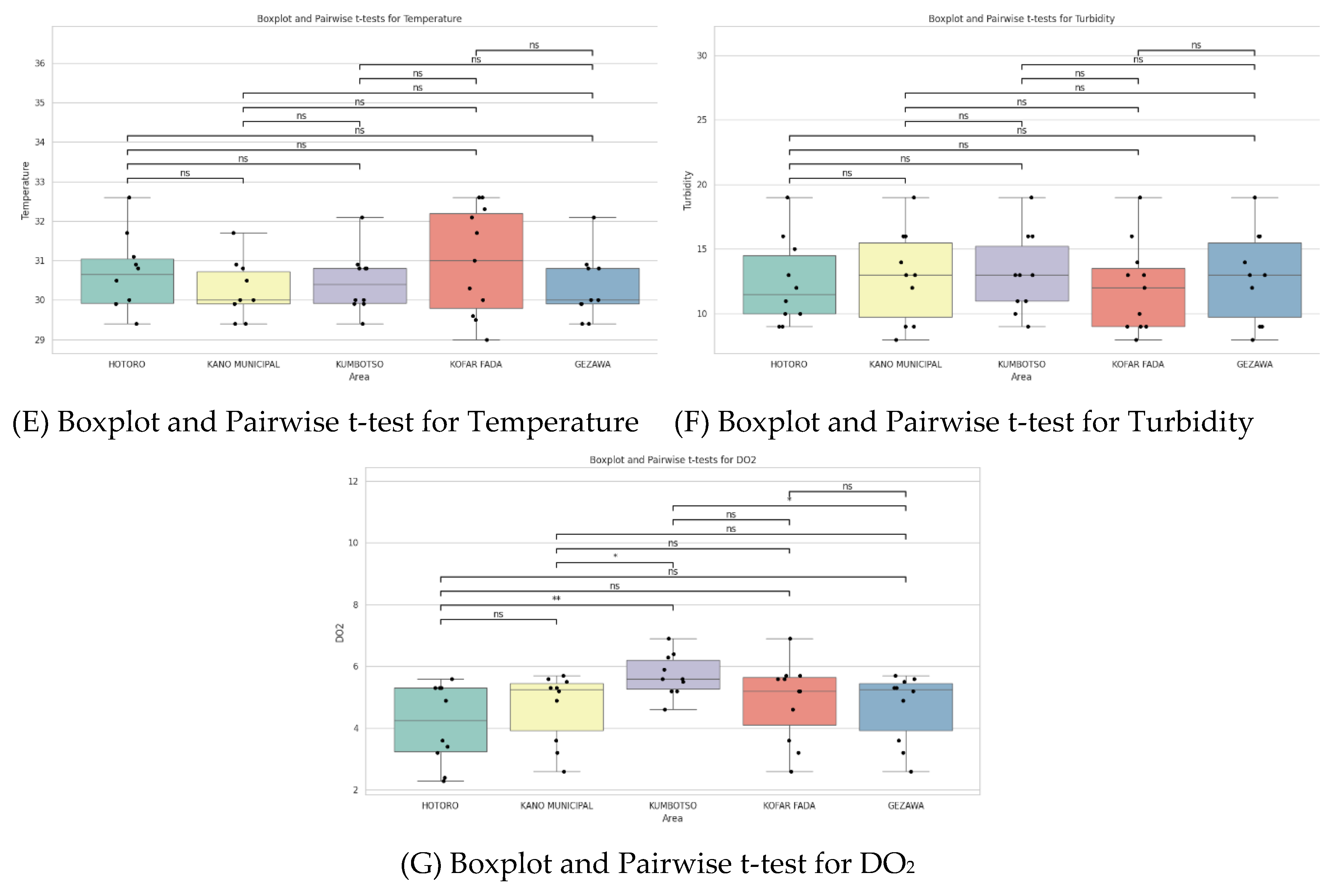
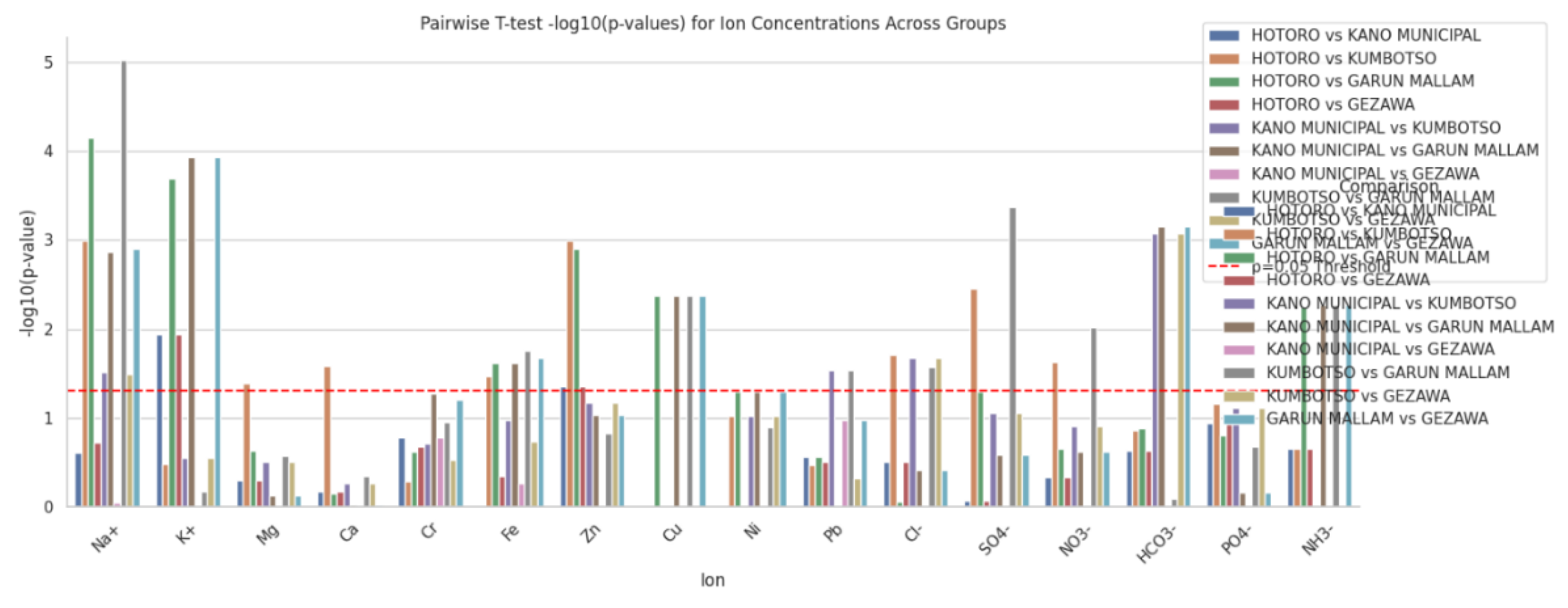
Figure 4.
Boxplot and Pairwise t-test for all the Cations and Anions in the study area.
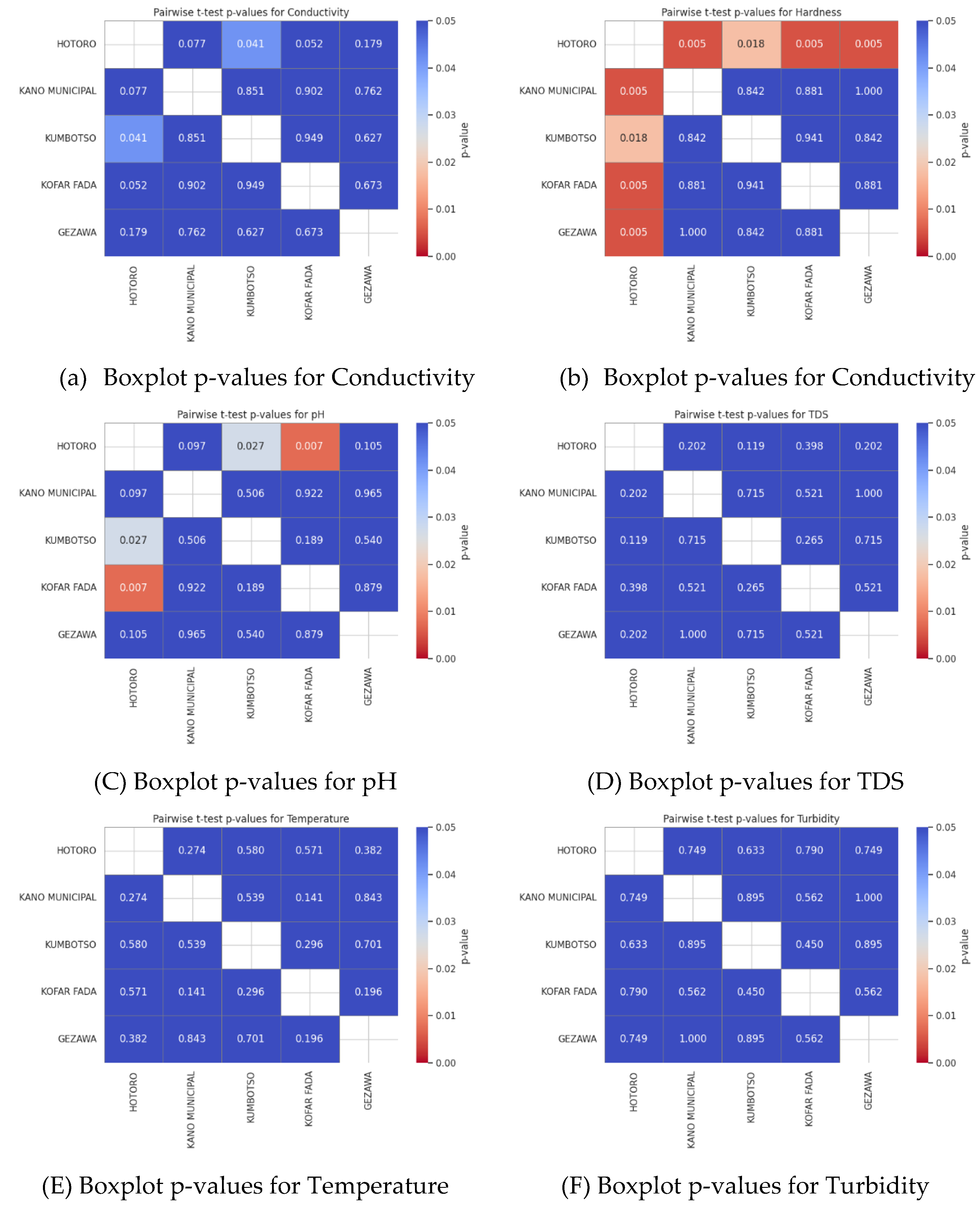
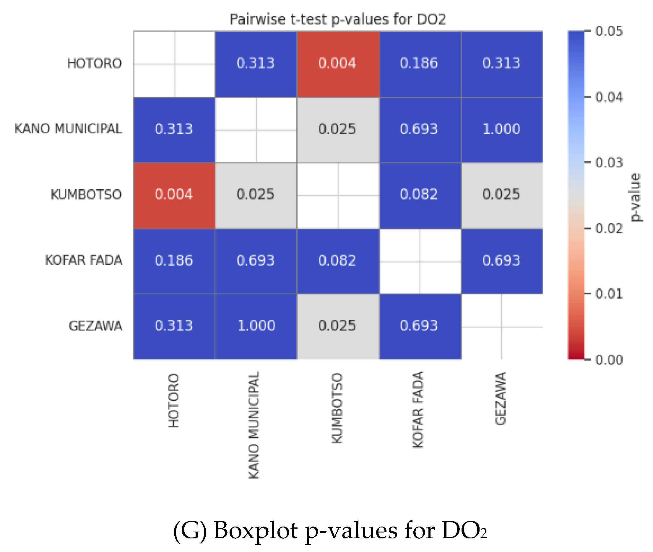
p-value plots Analysis
The heatmaps of p-value of the pairwise t-tests indicate which parameters of water quality are significantly different between the five regions of HOTORO, KANO MUNICIPAL, KUMBOTSO, KOFAR FADA, and GEZAWA. Statistically significant difference is reported by the low p-values (usually < 0.05) that underline the spatial heterogeneity of water quality. Conductivity, TDS, and hardness are parameters that are usually very different in more built-up or industrialized areas (such as HOTORO) compared to the less affected ones. On the other hand, the parameters with large p-values indicate some areas of similarity in terms of water quality. The visualizations assist in setting priorities of areas where targeted water management or pollution abatement is required, which are premised on underlying geology and human influences on water chemistry.
Figure 5.
showing (a) Boxplot p-values for Conductivity, (b) Boxplot and p-values for Conductivity, (C) Boxplot p-values for pH, (d) Boxplot p-values for TDS, € Boxplot p-values for Temperature, (f) Boxplot p-values for Turbidity, and (G) Boxplot p-values for DO2.
Figure 5.
showing (a) Boxplot p-values for Conductivity, (b) Boxplot and p-values for Conductivity, (C) Boxplot p-values for pH, (d) Boxplot p-values for TDS, € Boxplot p-values for Temperature, (f) Boxplot p-values for Turbidity, and (G) Boxplot p-values for DO2.
Confidence interval plots
The Confidence interval plot of water quality parameters of HOTORO, KANO MUNICIPAL, KUMBOTSO, KOFAR FADA, and GEZAWA shows the estimate of the mean with the range of uncertainty at a typical 95 percent confidence level. Narrower intervals mean that the measurements are consistent and reliable in an area, whereas wider intervals mean there is much variability or a smaller amount of data. Disagreement of the mean value and the non-overlapping confidence interval between areas indicates the existence of a statistically significant difference between the areas regarding water quality (e.g., conductivity or TDS), and this may be attributed to spatial heterogeneity attributable to either geology or anthropogenic activity. All in all, these plots give effective, scientifically powerful visual summaries to compare the water quality status with amplified confidence across regions and make sharply focused management decisions.
Figure 6.
(a) Mean & 95% Confidence interval of Conductivity, (b) Mean & 95% Confidence interval of Hardness, (c) Mean & 95% Confidence interval of Hardness pH, (d) Mean & 95% Confidence interval of TDS, (e) Mean & 95% Confidence interval of Temperature, (f) Mean & 95% Confidence interval of Turbidity and (g) Mean & Confidence interval of DO2.
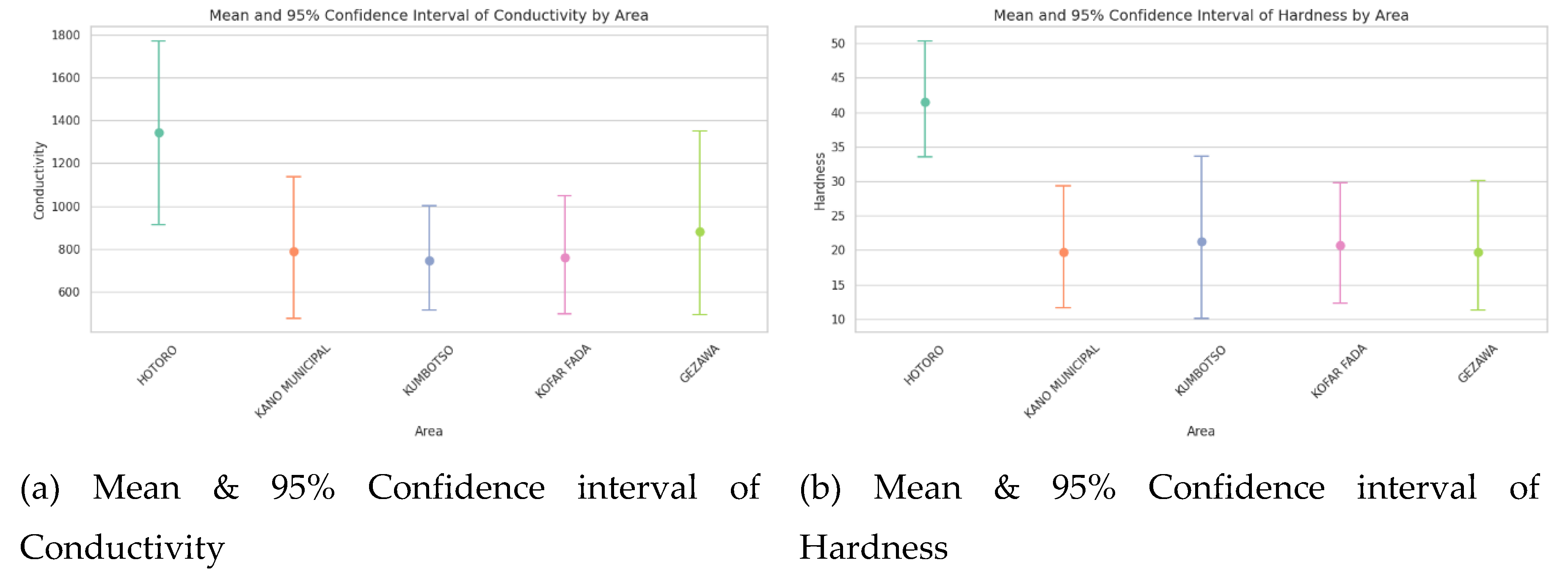
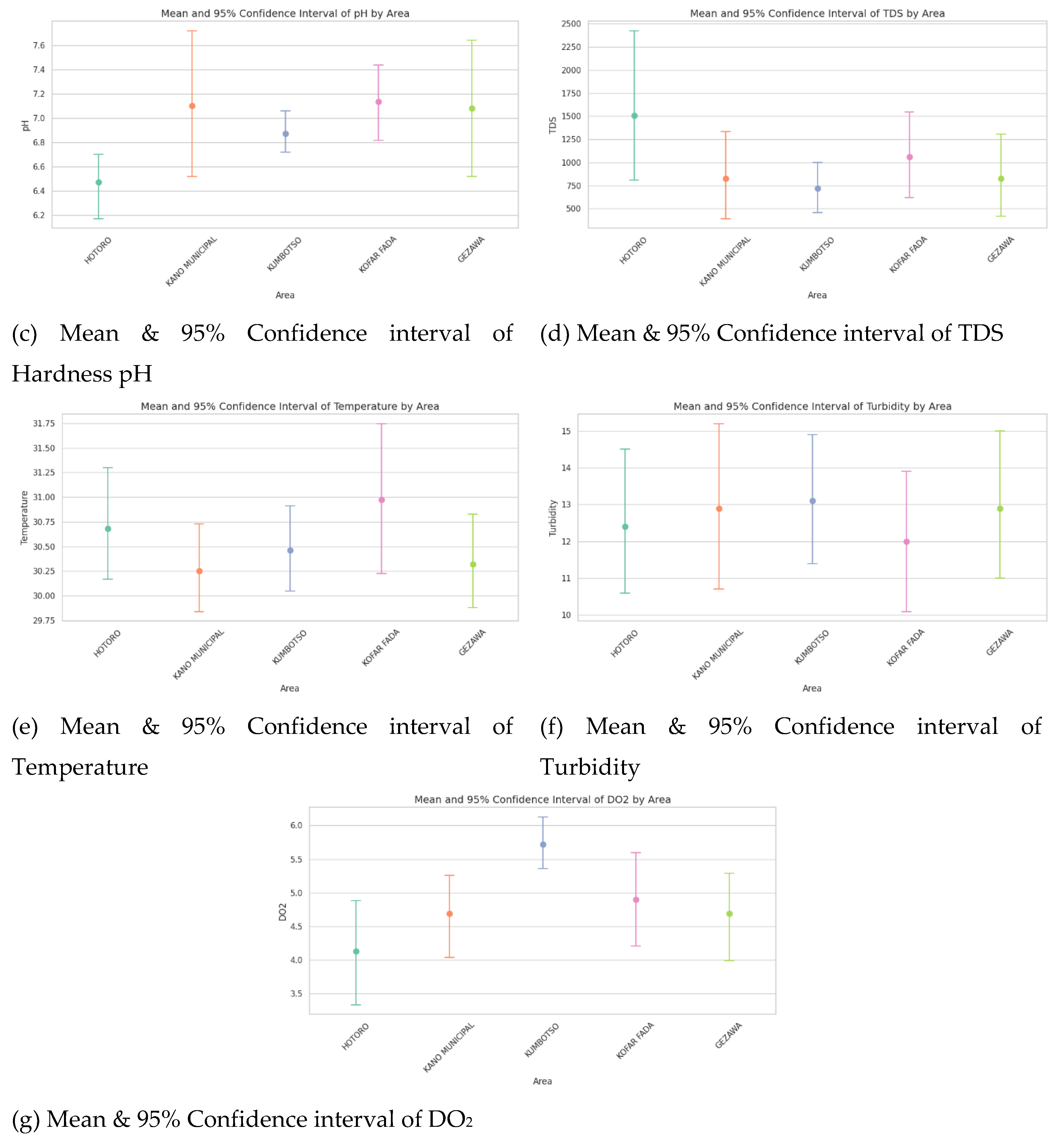
Table 2.
Showing Locations with Cation Concentration in the Study Area.
| S/No | Name | Na+ | K+ | Mg2+ | Ca2+ | Cr | AS | Fe | Zn | Cu | Ni | Pb | Cd |
|---|---|---|---|---|---|---|---|---|---|---|---|---|---|
| (Meq) | |||||||||||||
|
1 |
Sabon bakin zuwo Hotoro GRA | 23.4 | 0.1 | 23.2 | 16.4 | 0.0 | 0.0 | 0.01 | 0.0 | 0.0 | 0.0 | 0.00 | 0.0 |
| No. 6 Hotoro Avenue | 21.6 | 0.2 | 9.2 | 8.5 | 0.0 | 0.0 | 0.0 | 0.0 | 0.0 | 0.0 | 0.00 | 0.0 | |
| Hotoro | 20.4 | 0.0 | 34.2 | 9.6 | 0.04 | 0.0 | 0.01 | 2.51 | 0.4 | 0.0 | 0.004 | 0.0 | |
| No. 1 Sabo Bakin Zuwo Road. | 26.6 | 0.0 | 54.2 | 10.2 | 0.0 | 0.0 | 0.02 | 1.63 | 0.3 | 0.0 | 0.003 | 0.0 | |
| No. 13 Sabo Bakin Zuwo Road | 45.9 | 0.0 | 13.2 | 9.3 | 0.01 | 0.0 | 0.03 | 3.31 | 0.6 | 0.0 | 0.003 | 0.0 | |
| Tarauni | 54.9 | 0.0 | 15.6 | 16.1 | 0.0 | 0.0 | 0.0 | 1.60 | 0.0 | 0.0 | 0.10 | 0.0 | |
| Eastern Bypass Hotoro Kano | 61.3 | 0.1 | 11.5 | 12.2 | 0.0 | 0.0 | 0.04 | 2.61 | 0.2 | 0.0 | 0.002 | 0.0 | |
| No. 70 Ring Road Bypass | 34.1 | 0.2 | 10.3 | 16.6 | 0.01 | 0.0 | 0.04 | 1.56 | 0.5 | 0.0 | 0.002 | 0.0 | |
| No. 34 Ring Road Bypass | 23.6 | 0.3 | 9.5 | 9.5 | 0.0 | 0.0 | 0.001 | 1.23 | 0.0 | 0.0 | 0.001 | 0.0 | |
| Hotoro Kano | 21.6 | 0.2 | 15.6 | 12.9 | 0.0 | 0.0 | 0.0 | 1.65 | 0.0 | 0.0 | 0.00 | 0.0 | |
|
2 |
Kano Municipal 1 | 12.0 | 0.0 | 4.3 | 3.5 | 0.0 | 0.0 | 0.001 | 0.00 | 0.00 | 0.00 | 0.00 | 0.00 |
| Kano Municipal 2 | 31.0 | 0.0 | 5.2 | 9.1 | 0.0 | 0.0 | 0.001 | 0.00 | 0.00 | 0.00 | 0.00 | 0.00 | |
| Kano Municipal 3 | 15.4 | 0.0 | 6.2 | 5.5 | 0.0 | 0.0 | 0.002 | 0.04 | 0.002 | 0.00 | 0.00 | 0.00 | |
| Kano Municipal 4 | 12.5 | 0.0 | 5.2 | 4.2 | 0.0 | 0.0 | 0.001 | 0.14 | 0.00 | 0.00 | 0.00 | 0.00 | |
| Kano Municipal 5 | 10.4 | 0.0 | 5.2 | 6.5 | 0.0 | 0.0 | 0.001 | 0.45 | 0.00 | 0.00 | 0.00 | 0.00 | |
| Kano Municipal 6 | 54.1 | 0.0 | 6.2 | 4.3 | 0.0 | 0.0 | 0.002 | 0.10 | 0.00 | 0.00 | 0.00 | 0.00 | |
| Kano Municipal 7 | 12.5 | 0.0 | 6.5 | 3.5 | 0.0 | 0.0 | 0.001 | 0.31 | 0.00 | 0.00 | 0.001 | 0.00 | |
| Kano Municipal 8 | 10.6 | 0.0 | 16.3 | 12.6 | 0.001 | 0.0 | 0.06 | 3.01 | 0.00 | 0.00 | 0.003 | 0.00 | |
| Kano Municipal 9 | 45.1 | 0.0 | 56.2 | 34.2 | 0.004 | 0.0 | 0.04 | 1.03 | 0.00 | 0.00 | 0.002 | 0.00 | |
| Kano Municipal 10 | 43.3 | 0.0 | 36.3 | 23.4 | 0.001 | 0.0 | 0.04 | 1.30 | 0.001 | 0.00 | 0.005 | 0.00 | |
|
3 |
Kumbotso 1 | 12.0 | 0.02 | 6.4 | 9.1 | 0.00 | 0.00 | 0.01 | 0.00 | 0.0 | 0.00 | 0.001 | 0.00 |
| Kumbotso 2 | 5.1 | 0.00 | 10.3 | 15.0 | 0.02 | 0.00 | 0.00 | 0.00 | 0.0 | 0.00 | 0.005 | 0.00 | |
| Kumbotso 3 | 10.3 | 0.03 | 6.6 | 13.3 | 0.01 | 0.00 | 0.01 | 0.01 | 0.4 | 0.00 | 0.004 | 0.00 | |
| Kumbotso 4 | 16.4 | 0.54 | 12.6 | 6.5 | 0.00 | 0.00 | 0.00 | 0.01 | 0.3 | 0.00 | 0.003 | 0.00 | |
| Kumbotso 5 | 12.5 | 0.65 | 10.0 | 9.3 | 0.00 | 0.00 | 0.00 | 0.02 | 0.6 | 0.00 | 0.003 | 0.00 | |
| Kumbotso 6 | 14.0 | 0.02 | 11.0 | 6.9 | 0.00 | 0.00 | 0.00 | 0.10 | 0.0 | 0.00 | 0.00 | 0.00 | |
| Kumbotso 7 | 14.3 | 0.00 | 6.6 | 5.8 | 0.00 | 0.00 | 0.00 | 0.02 | 0. | 0.00 | 0.00 | 0.00 | |
| Kumbotso 8 | 10.3 | 9.50 | 9.5 | 4.9 | 0.00 | 0.00 | 0.00 | 0.01 | 0.0 | 0.00 | 0.00 | 0.00 | |
| Kumbotso 9 | 6.5 | 0.01 | 6.3 | 9.4 | 0.00 | 0.00 | 0.00 | 0.01 | 0.0 | 0.00 | 0.00 | 0.00 | |
| Kumbotso 10 | 6.1 | 0.00 | 8.2 | 5.3 | 0.00 | 0.00 | 0.00 | 0.01 | 0.0 | 0.00 | 0.00 | 0.00 | |
|
4 |
Aliko Oil Fueling Station | 0.00 | 1.83 | 6 | 5.61 | 0.00 | 0.00 | 0.1 | 0.04 | 0.7 | 0.00 | 0.00 | 0.00 |
| HJRBDA Office | 0.00 | 0.96 | 4 | 3.21 | 0.001 | 0.00 | 0.00 | 0.02 | 0.6 | 0.02 | 0.001 | 0.00 | |
| Kadawa Pri. Health Care | 0.00 | 1.88 | 7 | 6.11 | 0.00 | 0.00 | 0.2 | 0.02 | 0.0 | 0.00 | 0.00 | 0.00 | |
| Tangala | 0.00 | 2.67 | 31 | 24.63 | 0.003 | 0.00 | 0.4 | 0.02 | 0.0 | 0.02 | 0.003 | 0.00 | |
| Kofar Fada Jummat Mosque | 0.00 | 2.90 | 28 | 31.06 | 0.002 | 0.00 | 0.8 | 0.01 | 0.4 | 0.03 | 0.002 | 0.00 | |
| Makara Huta Borehole | 0.00 | 2.05 | 30 | 21.08 | 0.03 | 0.00 | 0.3 | 0.04 | 0.2 | 0.06 | 0.003 | 0.00 | |
| Rijiyar Isha’u | 0.00 | 0.64 | 9 | 5.86 | 0.004 | 0.00 | 0.2 | 0.26 | 0.1 | 0.01 | 0.004 | 0.00 | |
| Rijiyar Gidan Ganji | 0.00 | 0.66 | 8 | 5.62 | 0.005 | 0.00 | 0.0 | 0.00 | 0.2 | 0.00 | 0.005 | 0.00 | |
| Maza Waje Borehole | 1.40 | 0.91 | 6 | 5.69 | 0.081 | 0.00 | 0.0 | 0.32 | 0.3 | 0.00 | 0.081 | 0.00 | |
| Ali Yage Borehole | 0.00 | 0.89 | 4 | 4.99 | 0.036 | 0.00 | 0.0 | 0.02 | 0.1 | 0.00 | 0.036 | 0.00 | |
| Rijiyar Gidan Mallam Kabiru | 0.00 | 1.01 | 7 | 6.82 | 0.018 | 0.00 | 0.3 | 0.04 | 0.2 | 0.00 | 0.018 | 0.00 | |
|
5 |
Babawa 1 | 12.0 | 0.00 | 4.3 | 3.5 | 0.00 | 0.00 | 0.001 | 0.00 | 0.00 | 0.00 | 0.00 | 0.00 |
| Babawa 2 | 31.0 | 0.00 | 5.2 | 9.1 | 0.00 | 0.00 | 0.001 | 0.00 | 0.00 | 0.00 | 0.00 | 0.00 | |
| Kawaji | 15.4 | 0.00 | 6.2 | 5.5 | 0.00 | 0.00 | 0.002 | 0.04 | 0.00 | 0.00 | 0.00 | 0.00 | |
| Babawa 3 | 12.5 | 0.00 | 5.2 | 4.2 | 0.00 | 0.00 | 0.001 | 0.14 | 0.002 | 0.00 | 0.00 | 0.00 | |
| Kano, Gumel Road | 10.4 | 0.00 | 5.2 | 6.5 | 0.00 | 0.00 | 0.001 | 0.45 | 0.00 | 0.00 | 0.00 | 0.00 | |
| Babawa 4 | 54.1 | 0.00 | 6.2 | 4.3 | 0.00 | 0.00 | 0.002 | 0.10 | 0.00 | 0.00 | 0.00 | 0.00 | |
| Gezawa 1 | 12.5 | 0.00 | 6.5 | 3.5 | 0.00 | 0.00 | 0.001 | 0.31 | 0.00 | 0.00 | 0.001 | 0.00 | |
| Gezawa 2 | 10.6 | 0.00 | 16.3 | 12.6 | 0.001 | 0.00 | 0.006 | 3.01 | 0.00 | 0.00 | 0.003 | 0.00 | |
| Babawa 7 | 45.1 | 0.00 | 56.2 | 34.2 | 0.004 | 0.00 | 0.04 | 1.03 | 0.00 | 0.00 | 0.002 | 0.00 | |
| Kawaji 2 | 34.3 | 0.00 | 36.3 | 23.4 | 0.001 | 0.00 | 0.04 | 1.30 | 0.001 | 0.00 | 0.005 | 0.00 |
Table 3.
Showing Locations with Anion Concentration in the study Area.
| S/No | Name | Cl- | SO4- | NO3- | HCO3- | PO2 4- | NH3- |
|---|---|---|---|---|---|---|---|
| (Meq) | |||||||
|
1 |
Sabon bakin zuwo Hotoro GRA | 0.34 | 0.2 | 0.0 | 13 | 0.0 | 0.0 |
| No. 6 Hotoro Avenue | 1.45 | 0.5 | 0.13 | 12 | 0.0 | 0.0 | |
| Hotoro | 1.21 | 54 | 6.9 | 16 | 0.0 | 0.01 | |
| No. 1 Sabo Bakin Zuwo Road. | 1.00 | 63 | 9.6 | 10 | 0.6 | 0.01 | |
| No. 13 Sabo Bakin Zuwo Road | 0.46 | 69 | 12.0 | 116 | 3.5 | 0.0 | |
| Tarauni | 0.13 | 13 | 0.1 | 23 | 0.5 | 0.0 | |
| Eastern Bypass Hotoro Kano | 0.54 | 49 | 16 | 241 | 1.6 | 0.01 | |
| No. 70 Ring Road Bypass | 0.21 | 68 | 12.9 | 432 | 0.3 | 0.0 | |
| No. 34 Ring Road Bypass | 0.04 | 23 | 0.2 | 13 | 0.34 | 0.03 | |
| Hotoro Kano | 0.01 | 16 | 0.1 | 14 | 0.23 | 0.21 | |
|
2 |
Kano Municipal 1 | 0.0 | 0.02 | 0.04 | 130 | 0 | 0.0 |
| Kano Municipal 2 | 0.0 | 0 | 0.6 | 112.3 | 0 | 0.0 | |
| Kano Municipal 3 | 0.0 | 0 | 0.3 | 134 | 0.02 | 0.0 | |
| Kano Municipal 4 | 0.0 | 0 | 0.5 | 95.4 | 0 | 0.0 | |
| Kano Municipal 5 | 1.45 | 0 | 0.5 | 122 | 0 | 0.0 | |
| Kano Municipal 6 | 2.41 | 0 | 0.6 | 65.3 | 0 | 0.0 | |
| Kano Municipal 7 | 1.45 | 0 | 0.2 | 56.6 | 0.03 | 0.0 | |
| Kano Municipal 8 | 0.34 | 123.1 | 34.52 | 256.3 | 0.4 | 0.0 | |
| Kano Municipal 9 | 1.68 | 140.6 | 56.3 | 316.2 | 0.2 | 0.02 | |
| Kano Municipal 10 | 1.46 | 134.3 | 13.6 | 255.6 | 0.4 | 0.0 | |
|
3 |
Kumbotso 1 | 0.04 | 0.01 | 0.51 | 11 | 0.0 | 0.0 |
| Kumbotso 2 | 0.05 | 0.63 | 0.13 | 16 | 0.0 | 0.0 | |
| Kumbotso 3 | 0.01 | 0.53 | 0.15 | 17 | 0.0 | 0.0 | |
| Kumbotso 4 | 0.02 | 0.13 | 0.46 | 19 | 0.1 | 0.0 | |
| Kumbotso 5 | 0.16 | 0.00 | 0.23 | 13 | 0.0 | 0.0 | |
| Kumbotso 6 | 0.13 | 0.06 | 0.25 | 16 | 0.1 | 0.0 | |
| Kumbotso 7 | 0.06 | 0.14 | 0.15 | 18 | 1.3 | 0.0 | |
| Kumbotso 8 | 0.26 | 0.45 | 0.16 | 19 | 0.0 | 0.0 | |
| Kumbotso 9 | 0.03 | 2.33 | 0.26 | 14 | 0.0 | 0.0 | |
| Kumbotso 10 | 0.05 | 6.45 | 0.54 | 18 | 0.0 | 0.0 | |
|
4 |
Aliko Oil Fueling Station | 0.7 | 16.5 | 0.9 | 0 | 0.1 | 0.9 |
| HJRBDA Office | 0.2 | 13.1 | 1.3 | 0 | 0.0 | 1.3 | |
| Kadawa Pri. Health Care | 0.0 | 10.4 | 4.1 | 8 | 0.1 | 4.1 | |
| Tangala | 0.1 | 16.5 | 1.9 | 48 | 1.3 | 1.9 | |
| Kofar Fada Jummat Mosque | 1.4 | 10.4 | 1.4 | 57 | 0.0 | 1.4 | |
| Makara Huta Borehole | 1.0 | 9.3 | 9.3 | 32 | 0.0 | 9.3 | |
| Rijiyar Isha’u | 0.6 | 16.8 | 2.0 | 14 | 0.0 | 2.0 | |
| Rijiyar Gidan Ganji | 0.1 | 36.0 | 2.9 | 0 | 0.1 | 2.0 | |
| Maza Waje Borehole | 1.9 | 25.5 | 6.8 | 0 | 0.0 | 2.9 | |
| Ali Yage Borehole | 0.3 | 14.1 | 3.8 | 0 | 0.1 | 6.8 | |
| Rijiyar Gidan Mallam Kabiru | 0.0 | 0.02 | 4.0 | 0 | 0.0 | 0.0 | |
|
5 |
Babawa 1 | 0.0 | 0.0 | 0.04 | 130.0 | 0.0 | 0.0 |
| Babawa 2 | 0.0 | 0.0 | 0.6 | 112.3 | 0.0 | 0.0 | |
| Kawaji | 0.0 | 0.0 | 0.3 | 134.0 | 0.02 | 0.0 | |
| Babawa 3 | 0.0 | 0.0 | 0.5 | 95.4 | 0.0 | 0.0 | |
| Kano, Gumel Road | 1.45 | 0.0 | 0.5 | 122.0 | 0.0 | 0.0 | |
| Babawa 4 | 2.41 | 0.0 | 0.6 | 65.3 | 0.0 | 0.0 | |
| Gezawa 1 | 1.45 | 0.0 | 0.2 | 56.6 | 0.03 | 0.0 | |
| Gezawa 2 | 0.34 | 123.1 | 34.52 | 256.3 | 0.4 | 0.0 | |
| Babawa 7 | 1.68 | 140.6 | 56.3 | 316.2 | 0.2 | 0.02 | |
| Kawaji 2 | 1.46 | 134.3 | 13.60 | 255.6 | 0.4 | 0.0 | |
The table contains the details of the major cations (Na+, K+, Mg2+, Ca2+), trace/toxic elements (Chromium, Arsenic, Iron, Zinc, Copper, Nickel, Lead, Cadmium), and their concentrations in different groundwater sites. The major ion chemistry is largely dominated by sodium, magnesium, and calcium, whose levels greatly vary between sites; sodium is relatively high at Tarauni and Eastern Bypass Hotoro Kano, whereas magnesium and calcium are high at some Hotoro and Kumbotso locations. There is a generally low value of Potassium that is characteristic of natural waters because of its reactivity in soils. The trace metal and heavy metal analysis shows that most samples have an undetectable or extremely low concentration of chromium, arsenic, copper, nickel, lead, and cadmium, and this poses little risk of acute response to the elements, given the current circumstances. The presence of iron is sometimes observed in low concentrations, and that is not uncommon in groundwater and can be connected with the mineralogy of the aquifer. Zinc intermittently trends upwards, particularly in Hotoro and some of the Kano municipal samples, and this could be indicative of localized anthropogenic enrichment or natural fluctuation, but there appear to be very minimal levels of metals that could be considered harmful. The spatial heterogeneity indicates environmental importance when there are spiked sodium, magnesium, calcium, or zinc levels at certain sites (e.g., No.13 Sabo Bakin Zuwo Road, Eastern Bypass Hotoro Kano, Babawa 7) and hence any of these attributes is attributable to the geology, land use, or potential pollution. Nevertheless, the general outline of trace metals indicates generally safe water as regards the emission of heavy metals. Persistent monitoring should also be necessary, as occasional surges in metals such as Pb, Fe, and Zn, particularly in affected areas, may indicate episodic contamination events or changing land-use demands.
Correlation plot
In Hotoro, the correlation matrix demonstrates linear relationships that suggest common sources or geochemical behaviors. Notably, ions such as Na+, Cl-, and SO42- show strong positive correlations, indicating their joint origin, likely from geochemical processes or pollution sources. The heatmap facilitates quick identification of ion groups that co-occur, aiding in understanding water chemistry dynamics and potential environmental impacts.
Kano Municipal's correlation plot emphasizes interactions among ions like Na+, Mg, and Ca, which are indicative of mineral dissolution and water-rock interactions. High positive correlations denote shared geochemical controls, while low or zero correlations suggest independent sources or processes. Negative correlations, though less prominent, could highlight contrasting behaviors or contamination influences, guiding resource management and pollution assessment.
In Kumbotso, the correlation analysis underscores the interconnectedness of ions such as Mg and Ca, which tend to vary together due to similar geochemical controls. The heatmap visualizes these relationships, assisting in deciphering water chemistry trends and contamination impacts, essential for environmental decision-making.
Garun Mallam’s data reveals strong positive correlations between alkaline earth metals (Mg, Ca) and major ions like K+, signifying common natural sources like mineral dissolution. Conversely, trace metals and some ions show weak or null correlations, pointing to different sources or limited contamination. The correlation matrix supports targeted environmental evaluations and resource management strategies.
Gezawa's correlation plot depicts high positive relationships among major cations (Ca, Mg, Na), reflecting their origin from water-rock interactions. Trace metals such as Fe, Zn, and Pb exhibit weaker correlations, suggesting diverse sources or localized contamination. The visualization aids in identifying parameters that co-vary, informing environmental monitoring and pollution control efforts.
Collectively, these correlation analyses across all localities provide a comprehensive understanding of the interactions among water quality constituents. They highlight shared sources, geochemical behaviors, and potential pollution influences, serving as crucial tools for environmental assessment, resource management, and pollution mitigation strategies in the respective communities (Figure 7).
The spatial analysis of environmental parameters reveals significant variability across the surveyed region. Conductivity exhibits high spatial heterogeneity, with zero values at some locations and peaks mainly in central areas, indicating diverse mineral content, soil salinity, and environmental influences. Such variability necessitates advanced geostatistical methods like kriging for accurate mapping and resource assessment. Similarly, pH values range from approximately 5.6 to 8.7, with zero boundary values, reflecting heterogeneous soil and water conditions influenced by mineral weathering, organic matter decomposition, and microbial activity. This heterogeneity, with regions of acidity and alkalinity, impacts nutrient cycling, microbial processes, and environmental health, requiring localized evaluation and geostatistical modeling for effective management. Total Dissolved Solids (TDS) demonstrate substantial spatial variation, with boundary zeros and maximum values up to 4917 mg/L, indicating complex geochemical and pollutant distributions that influence water quality and ecological safety. Monitoring is essential to identify sources of mineralization or contamination. Temperature remains moderately stable, ranging from 29°C to 33°C, with minor local fluctuations caused by land cover, microclimate, and shading effects. These temperature patterns influence ecological processes like evapotranspiration and species distribution, informing urban planning and climate mitigation strategies.
Turbidity levels are moderate (8-19 NTU), predominantly along edges, indicating a stable presence of suspended particles that can impair aquatic life by reducing light penetration and conveying pollutants. Elevated turbidity can harm ecosystems, necessitating ongoing monitoring and actions to control erosion and runoff. Dissolved oxygen (DO2) varies from 2.3 to 6.9 mg/L internally, with boundary zeros, suggesting generally moderate water quality but localized hypoxia near 2.3 mg/L. These patterns highlight the influence of biological activity, organic matter decomposition, and environmental factors, serving as critical indicators for ecosystem health, pollution detection, and management efforts to preserve aquatic biodiversity and water quality. Overall, these parameters underscore the importance of geostatistical approaches for precise mapping, prediction, and sustainable environmental management (Figure 8).
The spatial variability of sodium (Na⁺) concentrations ranges from 0 to approximately 61.3 mg/L, with many boundary points showing zero values, indicating influences from geology, mineral weathering, evaporation, and human activities. While most levels are below health concern thresholds, localized peaks suggest areas needing monitoring due to potential impacts on water quality, soil health, and ecosystem stability. Potassium (K⁺) levels are generally very low, with a maximum around 9.5 mg/L, implying possible nutrient deficiencies affecting plant growth and soil fertility, with occasional spikes likely from mineral weathering or fertilizer use. This diverse distribution emphasizes the need for site-specific soil and water management to address potential agricultural and ecological impacts. Magnesium (Mg²⁺) concentrations display significant spatial variation, from zeros at boundaries to peaks around 56.2 mg/L, driven by processes like mineral weathering and water-rock interactions, affecting water hardness, alkalinity, and ecological health. Continuous monitoring and geostatistical mapping are essential for managing magnesium’s influence on water and soil quality. Similarly, calcium (Ca²⁺) levels vary from zero at edges to over 34.2 mg/L, reflecting geochemical and anthropogenic influences. Calcium plays a crucial role in buffering acidity, stabilizing pH, supporting aquatic life, and promoting plant growth. Variations in calcium levels impact ecosystem productivity and stress, underscoring the importance of spatial surveillance and geostatistical analysis to manage soil fertility and water quality effectively (Figure 9).
The water quality data across the surveyed area reveal significant spatial variability in key chemical parameters, each with implications for environmental health. Chloride (Cl⁻) concentrations are mostly low, generally below 2.5 mg/L, with many boundary points registering zero, suggesting minimal current contamination or salinity intrusion. However, elevated chloride levels can disrupt aquatic osmoregulation, impair reproduction, and contribute to soil salinization and infrastructure corrosion, highlighting the importance of ongoing geostatistical monitoring to prevent future buildup from sources like wastewater, road salts, or agriculture. Sulfate (SO₄²⁻) displays a heterogeneous distribution, with concentrations ranging from near zero at edges to over 140 mg/L internally. Elevated sulfate levels, resulting naturally from mineral weathering and volcanism but often intensified by human activities such as mining or industrial waste, can impact water taste, induce biogeochemical changes, and cause eutrophication and oxygen depletion, threatening aquatic ecosystems. Nitrate (NO₃⁻) levels vary widely, with most boundary points showing low or zero values, but localized hotspots reaching up to 56.3 mg/L, primarily from agricultural runoff and wastewater. High nitrates pose risks of eutrophication, harmful algal blooms, and health issues like methemoglobinemia, especially in infants. Many readings exceed regulatory limits, emphasizing the need for targeted management guided by geostatistical mapping. Bicarbonate (HCO₃⁻) exhibits high spatial heterogeneity, with null values at boundaries and peaks exceeding 400 mg/L centrally, indicating active geochemical processes such as rock erosion and carbonate mineral dissolution. Elevated bicarbonate influences carbon cycling, aquatic photosynthesis, and metal mobility, affecting water chemistry and toxicity risks, necessitating precise monitoring. Ammonia (NH₃) concentrations are predominantly low, but localized hotspots reach up to 9.3 mg/L, suggesting pollution sources like agriculture or wastewater. High ammonia levels can damage aquatic life, especially under high pH and temperature conditions, and promote harmful algal blooms, making detailed geostatistical mapping essential for ecosystem protection and water management (Figure 10).
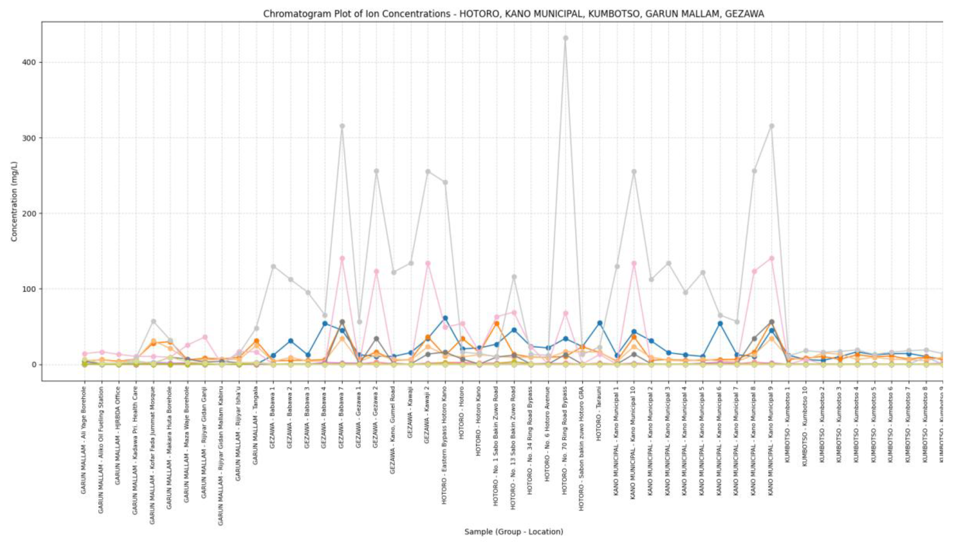
Chromatography: The chromatogram plot visually displays the concentration profiles of a wide range of ions and trace metals across multiple sampling sites from diverse locations such as HOTORO, KANO MUNICIPAL, KUMBOTSO, GARUN MALLAM, and GEZAWA. Each ion’s concentration is plotted as a line with markers spanning the various samples, making it straightforward to observe spatial trends, peaks, and relative abundances. This form of visualization highlights how concentrations of major cations (like Na+, Ca2+, Mg2+), anions (Cl-, SO4-, NO3-, HCO3-), and trace metals (Fe2+, Zn2+, Pb) vary from site to site, enabling identification of water quality patterns and potential contamination hotspots. The grouped x-axis by geographic areas helps compare water chemistry between regions at a glance. Such chromatogram plots serve as integration tools for complex multi-ion water quality data, effectively summarizing the chemical fingerprints of the sampled waters. Peaks in specific ions suggest elevated levels that may be driven by natural geochemical processes like mineral dissolution or anthropogenic activities such as industrial discharge or agricultural runoff. By simultaneously displaying numerous ions, the plot fosters a holistic interpretation of water composition and potential inter-ion relationships, informing environmental monitoring, groundwater resource management, and remediation strategies. Overall, chromatogram plots facilitate quick assessment of water chemistry variability and serve as a visual basis for more detailed hydrochemical analysis. This approach is a standard and established method in water quality laboratory analysis and monitoring.
Figure 11.
Chromatography plot of the study is. The chromatogram plot reveals distinct spatial variation in ion and trace metal concentrations across the sampling sites from HOTORO, KANO MUNICIPAL, KUMBOTSO, GARUN MALLAM, and GEZAWA areas. Major ions such as Na+, Ca, Mg, and HCO3- show consistent presence but with noticeable peaks indicating localized geochemical influences or contamination. Trace metals like Zn and Fe exhibit elevated levels at certain locations, suggesting possible anthropogenic inputs or mineralogical differences. Overall, the plot highlights diverse hydrochemical signatures reflecting natural and human impacts on groundwater quality across the different regions (Figure 11).
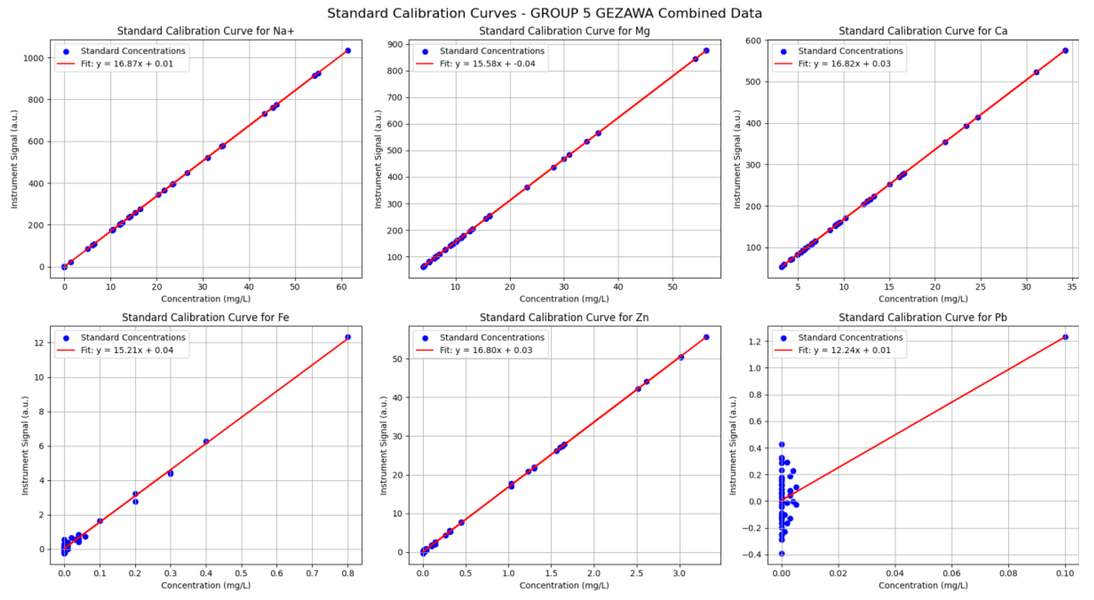
Standard Calibration Curve: The Standard Calibration Curve plot is used to draw the pattern of known anion concentrations and their relative instrument signals; usually, a linear regression is fitted to such data. Considering the validity of your combined water quality data, the curves show that the responses of the instrument across the measured ranges of key ions such as Na+, Mg, Ca, Fe, Zn, and Pb increase proportionally to concentration. The linearity supports the need to assume that concentration and signal relate to each other directly and predictably, which is the guiding principle of quantitative analysis in unknown samples. Fitted plot lines depict the span of the scattered points of data, and slopes and intercepts are estimated by the regression analysis, which hence aids in computing the sample concentration based on the instrument signals. The effectiveness of these calibration curves is evidenced by the low degrees of spread of data points about the regression lines, which establishes good measurement accuracy and good reproducibility of instruments. Well-spaced standard concentrations with a wide range will minimize uncertainty in slope and intercept estimates, thus higher and better quantifications. These calibration curves can also be used as an aid to diagnose whether there is a deviation in ideal behaviour, i.e., there is nonlinearity or a large amount of noise, and then more evaluation of the analytical method would be necessary. On the whole, the Standard Calibration Curve graph is one of the core work instruments in analytical chemistry, as this allows conducting a robust and true quality of water analysis since it is a graph towards links the instrumental output to actual ion concentrations.
Figure 12.
Standard Calibration Curve: The Standard Calibration Curve graph shows that there is a high linear correlation of the ion concentration (Na+, Mg2+, Ca2+, Fe2+, Zn2+, Pb2+) against the instrument signal, thus the quantitative analysis of it is precise. The small area of scatter about the lines shows that there is good precision and certainty of the measurement consistency. Fluctuations on the slope of the ions indicate a disparity in the sensitivity of the instrument to both analytes. On the whole, the calibration curves confirm the appropriateness of the analytical method to be used in terms of defining the water quality of varied sample groups (Figure 12).
Scatter plot: Analysis based on the scatter plot of all generic water quality data of HOTORO, KANO MUNICIPAL, KUMBOTSO, GARUN MALLAM, and GEZAWA shows that the pair of selected ions was linked and had co-variations in varied locations. The scatter diagram can be used in plotting the major ions, such as Na+ against Mg, Ca vs Mg, and Zn versus Fe can help to find the positive consistency between major cations, which is most likely due to a common geological or hydrochemical origin, e.g., mineral dissolution and water-rock reaction. At the same time, other trace metals, including Zn and Fe, are variable, bringing out local geochemistry or manmade effects. The clustering of points based on location using different colors is also useful in the visual identification of regional differences in hydrochemical signatures. The scatter plot can also be used as an exploratory tool for the assessment of water quality, as it can show small groups of several samples with similar ionic compositions and possibly outliers that can point to the contamination or abnormal geochemical state. The trends noted in these scatter plots can also be used to assist in the multivariate analyses, which are presented in the form of principal component analysis, which ascertains the interpretation of complex data more efficiently. In general, this kind of visualization is the accepted and very effective method of environmental chemistry used to diagnose spatial variability in water chemistry and inform local monitoring or remediation. This is in tandem with conventional wisdom that scatter plots can give a quick look as to whether water quality parameters are linearly or non-linearly related to each other, and that this information can guide holistic planning over water resources (Figure 13).
Principal Component of Curve: The Principal Component Curve graph prepared using the consolidated data of water quality of HOTORO, KANO MUNICIPAL, KUMBOTSO, GARUN MALLAM, and GEZAWA gives an account of consolidating multidimensional information on ion concentration into two principal components (principal element 1 and principal element 2) that represent the maximum of the variances. This dimensionality reduction shows important patterns and clusters in the dataset, and samples close to one another in the plot have comparable water chemistry profiles. Percentages of explained variance of PC1 and PC2 show the percentage of the overall variability in data that any of the PCs explain, giving an idea of the prevailing factors leading to the variation of the water quality over these areas. Also, the spatial distribution of groups by color samples on the PCA plot shows that each place has its own hydrochemical characteristics and possible natural or artificial factors that may affect it. The closer the two samples are, the more they tend to have similar ionic compositions, and conversely, the farther apart they are, the more different the water quality characteristics. The loadings (not included in the plot) behind these principal components normally indicate which ions are most responsible for these variations, and can therefore be used to guide further specific, environmentally or geochemically focused studies. On balance, this PCA visualization provides an efficient overview of complex datasets that can improve insights into the water chemistry variations in regions and enable data-based decisions to be made in managing the water resources (Figure 14).
The Piper plot analysis of the presented water chemistry data shows the presence of various hydrochemical facies along the sampled locations, as the focus of the spatial variability map is placed on the variability in ionic composition. The cation triangle indicates the prevalence of Sodium (Na+) and Potassium (K+) in a number of samples, especially the water types with high Sodium content (e.g., more than 40 meq/L), strongly suggesting the influence of sodium-bearing minerals or a source of high Sodium content due to anthropogenic activities. Mg2+ and Ca2+ reservoirs vary considerably; locations with elevated calcium and Magnesium indicate waters subjected to the dissolution of carbonate rock or groundwater-rock interaction with typical waters of the Calcium-Magnesium bicarbonate or sulfate water variety. The anion triangle reveals an aggregate of areas dominated by the abundance of bicarbonate (HCO3-), reflecting weak acid sites and other sites dominated by a high concentration of sulfate (SO4 2-) and chloride (Cl-), suggesting that the acidity is stronger due to industrial or agricultural contributions. These relative patterns of the various concentrations of these major ions give discrete groups or facies, indicating variations in conferring to the various geochemical processes such as silicate weathering, ion exchange, or source of contamination (Figure 15).
Discussion
The overall data regarding the quality of water in various sampling spots of the Kano area in Nigeria are characterized by a strongly heterogeneous environment of hydrochemical distribution pattern as a result of the intricate interplay of the lithological compositions of the land with urbanization and anthropogenic activities. The measured parameters; Electrical Conductivity, Hardness, pH, Total Dissolved Solids (TDS), Temperature, Turbidity and the Dissolved Oxygen (DO2), are spatially classified or confined between 802°-859° latitudes and 1100°-1214° longitudes, and reflect various physical, chemical, and biological water quality indicators that differ tremendously across the locations namely: Hotoro, Kano Municipal, Kumbotso, Kofar Fada and Gezawa. The values of conductivity were high, above 2400 1S/cm in urban areas such as Hotoro and Ring Road, and the results are similar to elevated TDS and Hardness, implying mineralization or anthropogenic pollution activities. Most pH values are in an acidic-alkaline range that is broadly acceptable as drinking water, but acidic at the borderline edge are of concern due to acidic corrosiveness and leaching of metals. Moderate fluctuations in turbidity (8-19 NTU) suggest fluctuating suspended solids that can degrade the visibility in a body of water and include possible disease-causing organisms, making it challenging to treat and stressing aquatic life. Temperature is also homogenous (29-33.39 °C) as per the tropical climatic conditions, with opposite effects on the Dissolved Oxygen that has a wide range (2.3-6.9 mg/L) and tends to be lower in the locations with high Conductivity and high Turbidity, indicating organic pollution or eutrophication-based hypoxia. Multivariate visualizations (Boxplots, Scatter plots, Violin plots, and Pairwise correlations) help explain parameter-specific spatial heterogeneities, and it is shown that the mineral and pollutant loads seem to be higher in the case of areas like Hotoro and the parts of Kumbotso, whereas Dissolved Oxygen concentrations are greater in those waters with the neutral to alkaline pH, further supporting beneficial aquatic conditions. Further investigations with t-tests and p-value heatmaps could also substantiate that there are large inter-site variations, at least in the conductivity, TDS, and Hardness data, which tend to underline the influence of urbanization on such aspects as geological heterogeneity.
The evidence of intervals represents the confidence of these findings and helps outline areas of need when it comes to interventions involving the quality of water. The ion chemistry profile is dominated by Sodium-Magnesium-Calcium, with site variation within the geological bodies, and is increased by anthropogenic effects. As such, Trace metals are present but at low concentrations and do not constitute immediate health hazards, though occasionally Zinc and Iron can be elevated, and hence need monitoring. Correlation matrices among localities strengthen geochemical processes of dissolution of minerals and interactions between water and rocks, as well as point to local wash-ups of contamination. Geostatistical analyses highlight excessive spatial heterogeneity of the most prominent physicochemical parameters, requiring the use of refined spatial analyses to drive adaptive management. Chromatogram plots that are used by the group combine multiple ion datasets to give a visual picture of spatial trends that are useful in establishing contamination hotspots as well as natural backgrounds. Calibration curves of analysis instruments testify to the robustness and precision of the ion quantifications. The major cation relationships illustrated with scatter plot analyses are consistent, indicating that major ion chemistry is consistent with geological origins; the principal component analysis allows effective reduction of the multivariate variability into clearly observable hydrochemical groupings that relate to geographic and manmade processes. Finally, Piper diagram analyses verify the convergence/divergence of several hydrochemical facies reflective of different geochemical processes, such as silicate weathering and carbonate dissolution, to anthropogenic enrichment of ions, which drive changes in the chemistry of water across sites. All these combined results highlight the essential role that real-time multifactor studies and spatially explicit management and mitigation measures must play to prevent water resource and aquatic living conditions in this fast-growing, highly populated Nigerian environment.
Conclusion
The high spatial heterogeneity of water quality is clearly expressed in the comprehensive study of water quality in various sampling locations in the Kano region in the Northern part of Nigeria due to complex interactions of the geological formations, eruptions of developmental activities, and anthropogenic pollution sources. Major parameters such as Electrical Conductivity, Hardness, pH, Total Dissolved Solids, Temperature, Turbidity, and Dissolved Oxygen help overall define the physical, chemical, and biological condition of the water and reveal localized hotspots of mineralization and contamination, especially in urban districts like Hotoro and some areas of Kumbotso. The high conductivity and TDS go along with an increased hardness and ion concentration to indicate ongoing geochemical processes in the waters (minerals dissolution) and anthropogenic impacts, including industrial effluents and agricultural runoffs. The values of pH are within the acceptable rates of drinking water, although borderline acidic conditions of certain sites express apprehensions of corrosion and leaching of metals. The changes in Turbidity and the reduction of available Dissolved Oxygen in some places signal a possible presence of pathogens as well as organic contamination, which impacts the health of water ecosystems. Multivariate statistical techniques (t-tests, Confidence intervals, Correlation matrices, Principal component analysis, and Piper diagrams) consistently show major disparities in water chemistries across the surveyed localities, whether of natural geochemical facies or of human-induced change. The concentration of trace metals is largely low concentrations and there is reduced direct effect on health, but there are periodic peaks that will require constant monitoring. The use of geostatistical techniques lends credence to the argument that to ensure the spatial differences of these often-changing issues of water quality, monitoring, and management must be spatially explicit. In sum, the combined multi-parameter assessment will promote the overall picture of the hydrochemical environment, which entails the necessity to maintain long-term and point-specific assessment of water quality and location-site interventions to maintain sustainable water usage management and sustainable aquatic ecosystems in the Kano territory. The Piper plot analysis of the presented water chemistry data shows the presence of various hydrochemical facies along the sampled locations, as the focus of the spatial variability map is placed on the variability in ionic composition. The cation triangle indicates the prevalence of Sodium (Na+) and Potassium (K+) in a number of samples, especially the water types with high Sodium content (e.g., more than 40 meq/L), strongly suggesting the influence of sodium-bearing minerals or a source of high Sodium content due to anthropogenic activities. Mg2+ and Ca2+ reservoirs vary considerably; locations with elevated calcium and Magnesium indicate waters subjected to the dissolution of carbonate rock or groundwater-rock interaction with typical waters of the Calcium-Magnesium bicarbonate or sulfate water variety. The anion triangle reveals an aggregate of areas dominated by the abundance of bicarbonate (HCO3-), reflecting weak acid sites and other sites dominated by a high concentration of sulfate (SO4 2-) and chloride (Cl-), suggesting that the acidity is stronger due to industrial or agricultural contributions. These relative patterns of the various concentrations of these major ions give discrete groups or facies, indicating variations in conferring to the various geochemical processes such as silicate weathering, ion exchange, or source of contamination (Figure 15).
References
- Abhijeet Das. (2025): An optimized approach for predicting water quality features and a performance evaluation for mapping surface water potential zones based on Discriminant Analysis (DA), Geographical Information System (GIS), and Machine Learning (ML) models in the Baitarani River Basin, Odisha. Desalination and Water Treatment. Pp1-22.
- Barath Kumar S; Padhi, R. K; Mohanty, A. K; Satpathy K. K. (2020): Distribution and ecological- and health-risk assessment of heavy metals in the seawater of the southeast coast of India. Marine Pollution Bulletin Volume 161, Part A, 111712. https://www.sciencedirect.com/science/article/abs/pii/S0025326X20308304 doi.org/10.1016/j.marpolbul.2020.111712.
- Bellal Hamma; Abdullah Alodah; Foued Bouaicha; Mohamed Faouzi Bekkouche; Ayoub Barkat; Enas E. Hussein. (2024): Hydrochemical assessment of groundwater using multivariate statistical methods and water quality indices (WQIs). Applied Water Science (2024) 14:33. Pp16-33. [CrossRef]
- Emoyan, O. O, Akpoborie, I., and Akporhonor, E. E. (2008): The Oil and Gas Industry and the Niger Delta: Implications for the Environment. J. Appl. Sci. Environ. Manage. https://www.researchgate.net/publication/27796899. Vol. 12(3) 29 - 37.
- Garba Ali Mohammed, Charles Calvin Kauda, Ezekiel Kamureyina, Mustafa Ali Garba, Musa Hayatudeen, Udo Aniedi Aniekan. (2024). Assessment of Bedrock Depth Utilizing Vertical Electrical Sounding (DDBR). International Journal of Emerging Science and Engineering (IJESE) ISSN: 2319–6378 (Online), Volume-12 Issue-12. Pp 5-12.
- Garba Ali Mohammed, Ganesh Prasad Singh, A. Olasehinde, and Ali Dawa Saidu. (2014). Study on the Physico-Chemical Characteristics of Groundwater in Michika Town and Environs, Northeastern Nigeria. Scientific Research Journal (SCIRJ), Volume II, Issue IV, April 2014 40 ISSN 2201-2796. Pp40-48.
- Ghoto Sher Muhammad, Habibullah Abbasi, Sheeraz Ahmed Memon, Khan Muhammad Brohi, Rabia Chhachhar, Asad Ali Ghanghlo, Imran Aziz Tunio: (2025): Multivariate hydrochemical assessment of groundwater quality for irrigation purposes and identifying soil interaction effects and dynamics of NDVI and urban development in an alluvial region. Environmental Advances 19 (2025) 100621. Pp1-19. [CrossRef]
- Hanaa A. Megahed1, Abd El-Hay A. Farrag, Amira A. Mohamed, Mahmoud H. Darwish, Mohamed A. E. AbdelRahman, Heba El-Bagoury, Paola D’Antonio, Antonio Scopa and Mansour A. A. Saad. (2025): GIS-based modeling and analytical approaches for groundwater quality suitability for different purposes in the Egyptian Nile Valley, a case study in Wadi Qena. DOI 10.3389/frwa 2025.1502169. PP 1-20.
- Ifie-emi Francis Oseke: (2025): Spatial Distribution of Pattern of Electrical Conductivity, Total Dissolved Solids, and Potential of Hydrogen Using GIS Techniques. Journal of Scientific and Engineering Research, 2025, 12(2):33-39.
- Jalal Valiallahi and Mahsa Yazdani. (2025): Evaluating groundwater quality by examining electrical conductivity, total dissolved solids, total hardness, and turbidity using geographic information systems (GIS®): a case study of selected wells in the Taleghan region, Iran. Applied Water Science (2025) 15:61, Pp 50-61. [CrossRef]
- Mohammed Sadid Hossain, Nazneen Nahar, Molla Rahman Shaibur, Md Tareq Bhuiyan, Abu Bakar Siddique, Abdullah Al Maruf, Abu Shamim Khan. (2024): Hydro-chemical characteristics and groundwater quality evaluation in the south-western region of Bangladesh: A GIS-based approach and multivariate analyses. ScienceDirect. Heliyon journal homepage: www.cell.com/heliyon. Pp1-15. [CrossRef]
- Musaab, A.A. Musaab A.A. Mohammed, Norbert P. Szab, Peter Szucs. (2022): Multivariate statistical and hydrochemical approaches for evaluation of groundwater quality in North Bahri City-Sudan. ScienceDirect. Heliyon journal homepage: www.cell.com/heliyon. Pp1-17. [CrossRef]
- Nayak Anjali, Gagan Matta, and D. P. Uniyal. (2022): Hydrochemical characterization of groundwater quality using chemometric analysis and water quality indices in the foothills of the Himalayas. [CrossRef]
- SuResh Nathan, N. Raravanane, R., and Sundararajan, T. (2017): Spatial Variability of Ground Water Quality Using HCA, PCA, and MANOVA at Lawspet, Puducherry in India. Computational Water, Energy, and Environmental Engineering, 2017, 6, http://www.scirp.org/journal/cweee. 243-268. [CrossRef]
- Odunayo Tope Ojo, Ike Joy Chiaka, Austin Emeka Okoli, and Namdie Joseph Inyang. (2025): Hydrochemical Assessment and Geospatial Analysis of Borehole Water Quality in Effurun, Delta State, Nigeria. AL-Bahir Journal for Engineering and Pure Sciences. 7, Pp7-24. [CrossRef]
- Oseke, I. F. (2025). Spatial distribution pattern of electrical conductivity, total dissolved solids, and potential of hydrogen using GIS techniques. Journal of Scientific and Engineering Research, 12(2), 33–39.
Figure 7.
Correlation plot in the study Area.
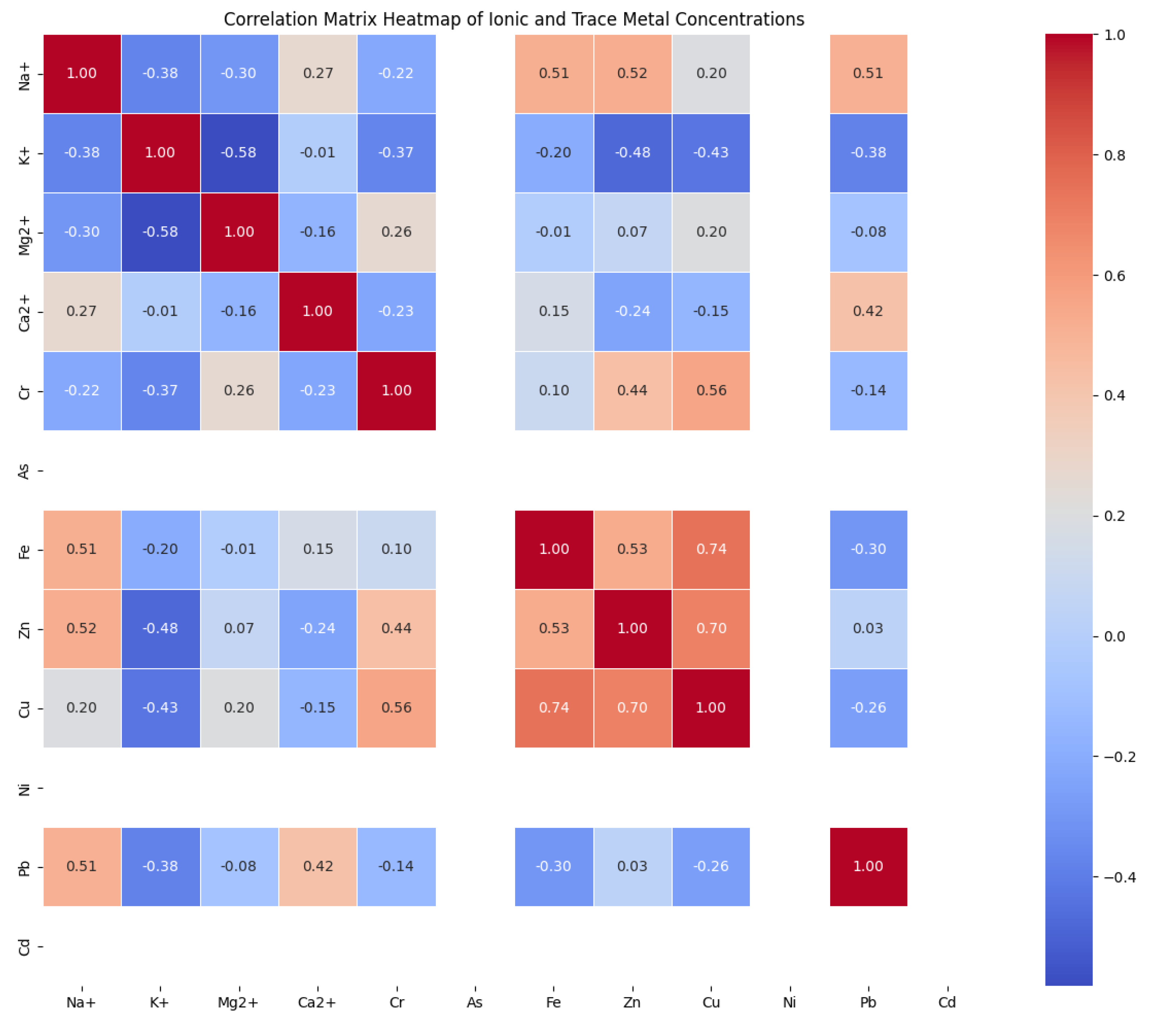
Figure 8.
(a) Conductivity Concentration, (b) Hardness Concentration, (c) pH Concentration, (d) TDS Concentration, (e) Temperature Concentration, (f) Turbidity Concentration, and (g) DO2 Concentration of the Study Area.
Figure 8.
(a) Conductivity Concentration, (b) Hardness Concentration, (c) pH Concentration, (d) TDS Concentration, (e) Temperature Concentration, (f) Turbidity Concentration, and (g) DO2 Concentration of the Study Area.
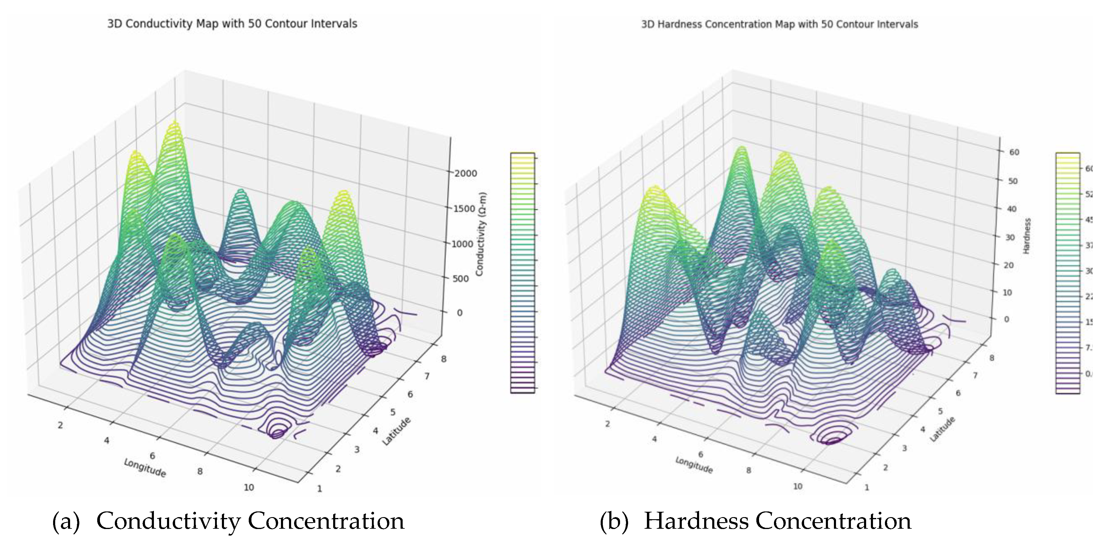
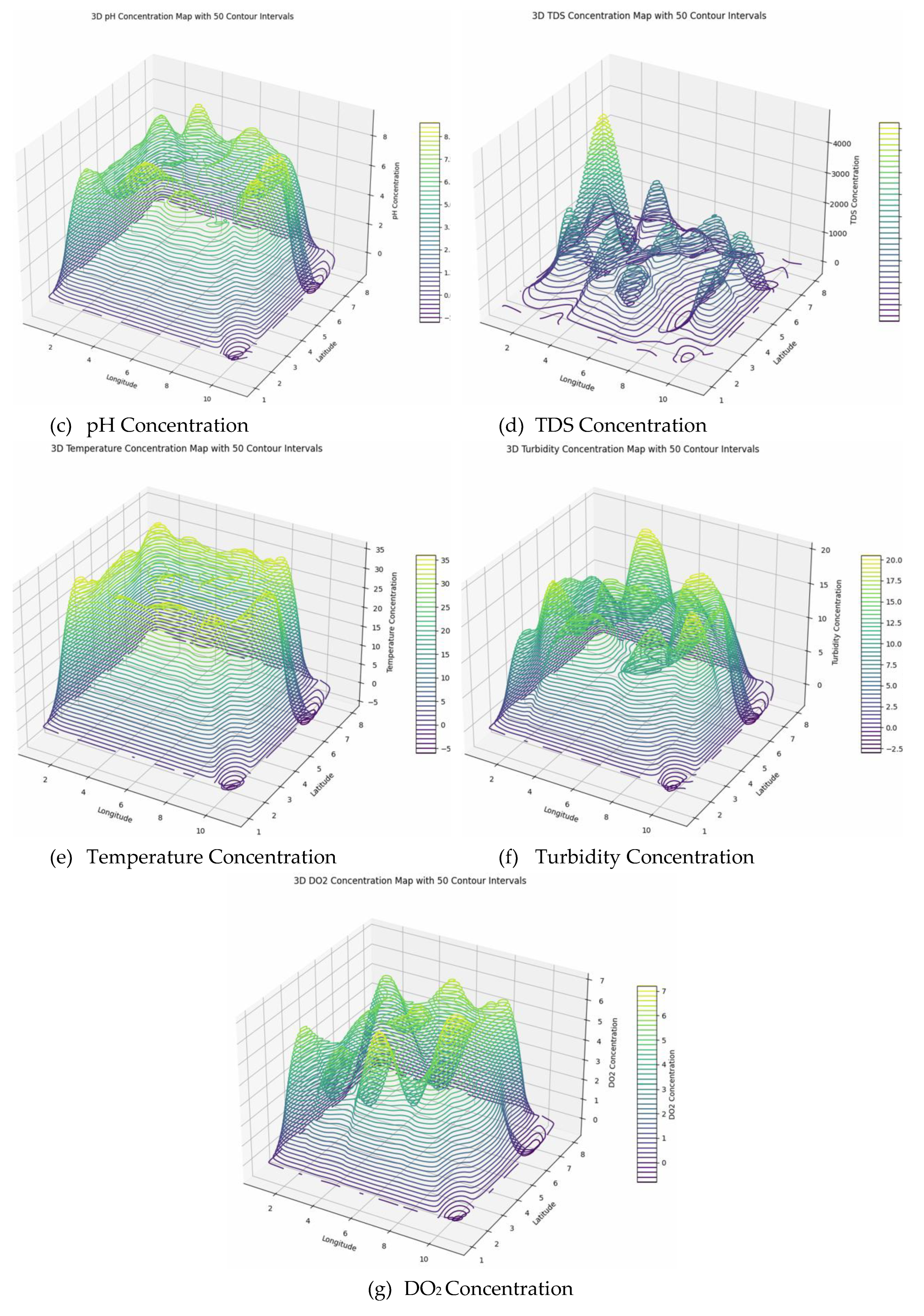
Figure 9.
Cation Concentration in (Meq) in the Study Area.
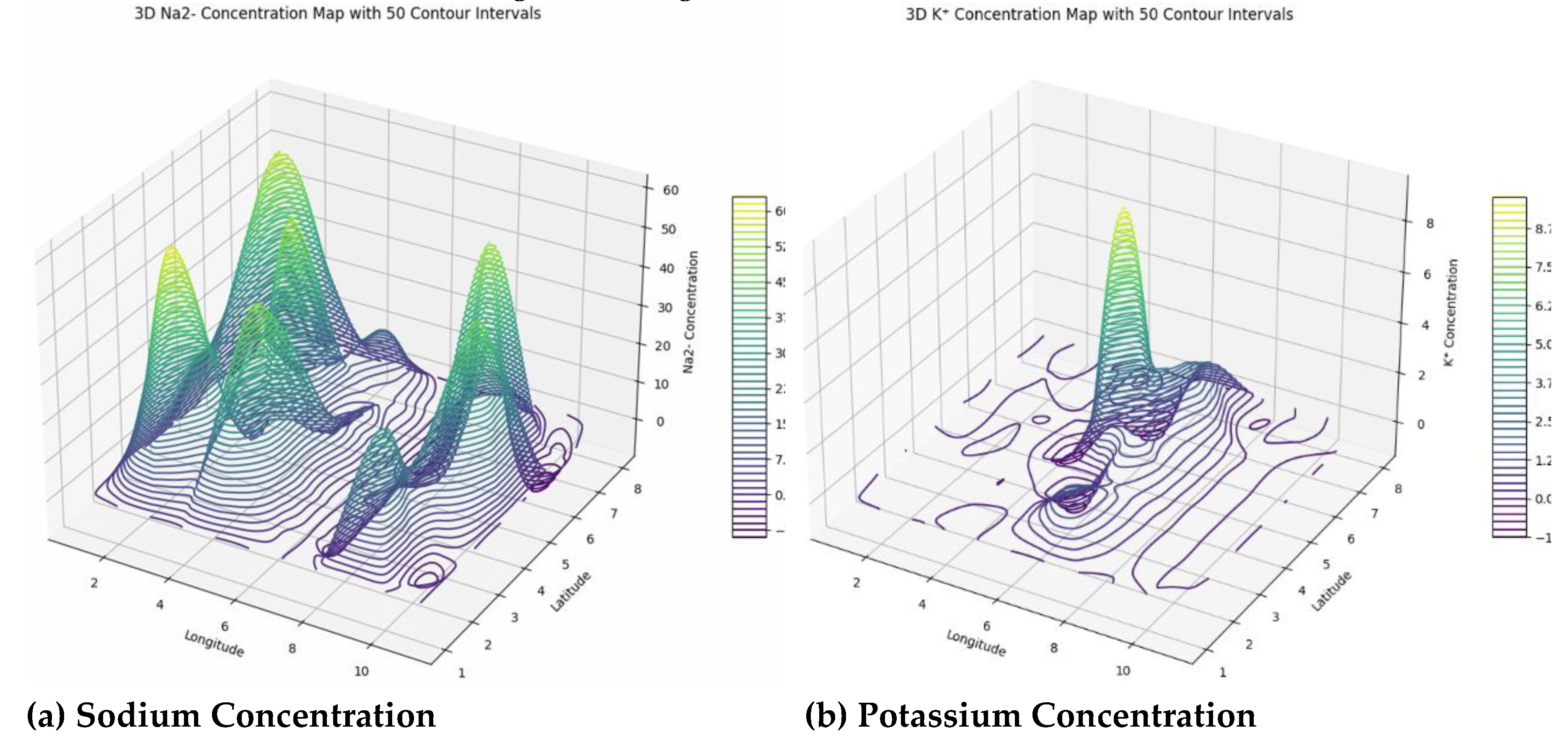
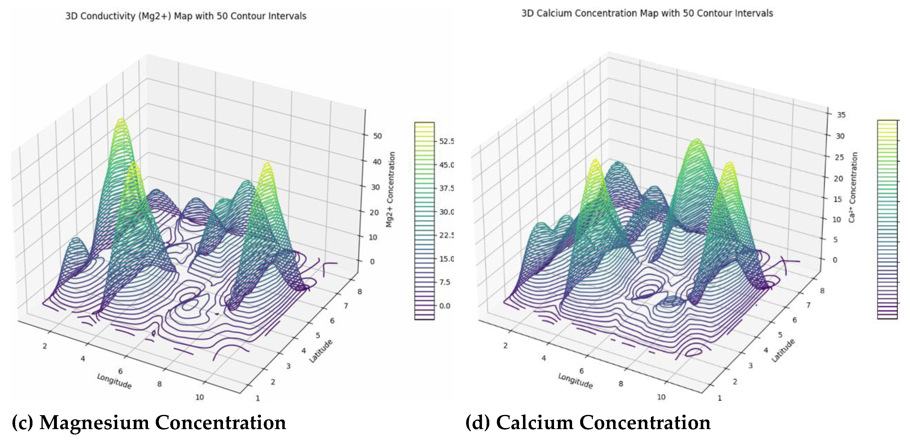
Figure 10.
Anion Concentration in (Meq) the Study Area.
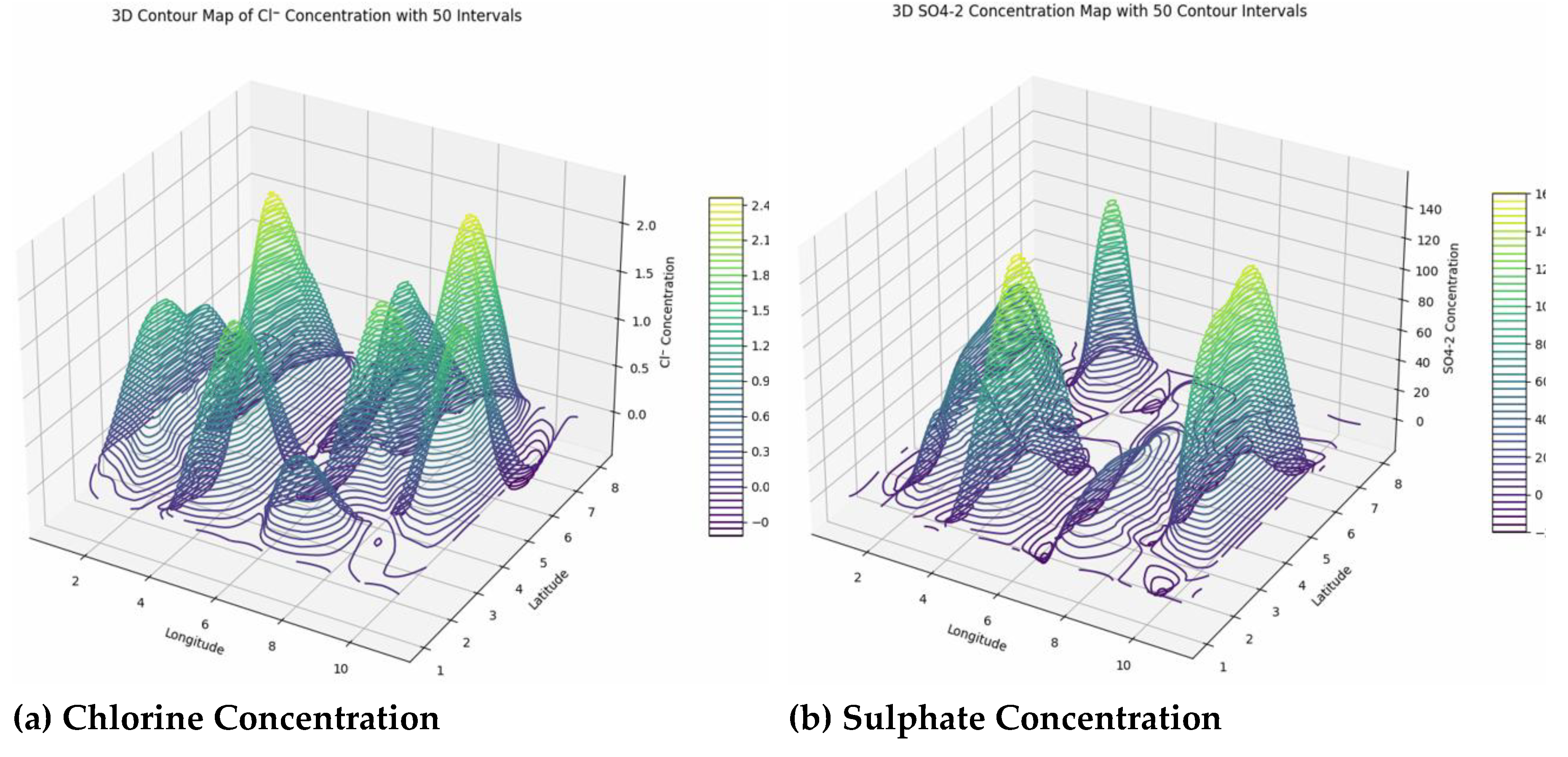
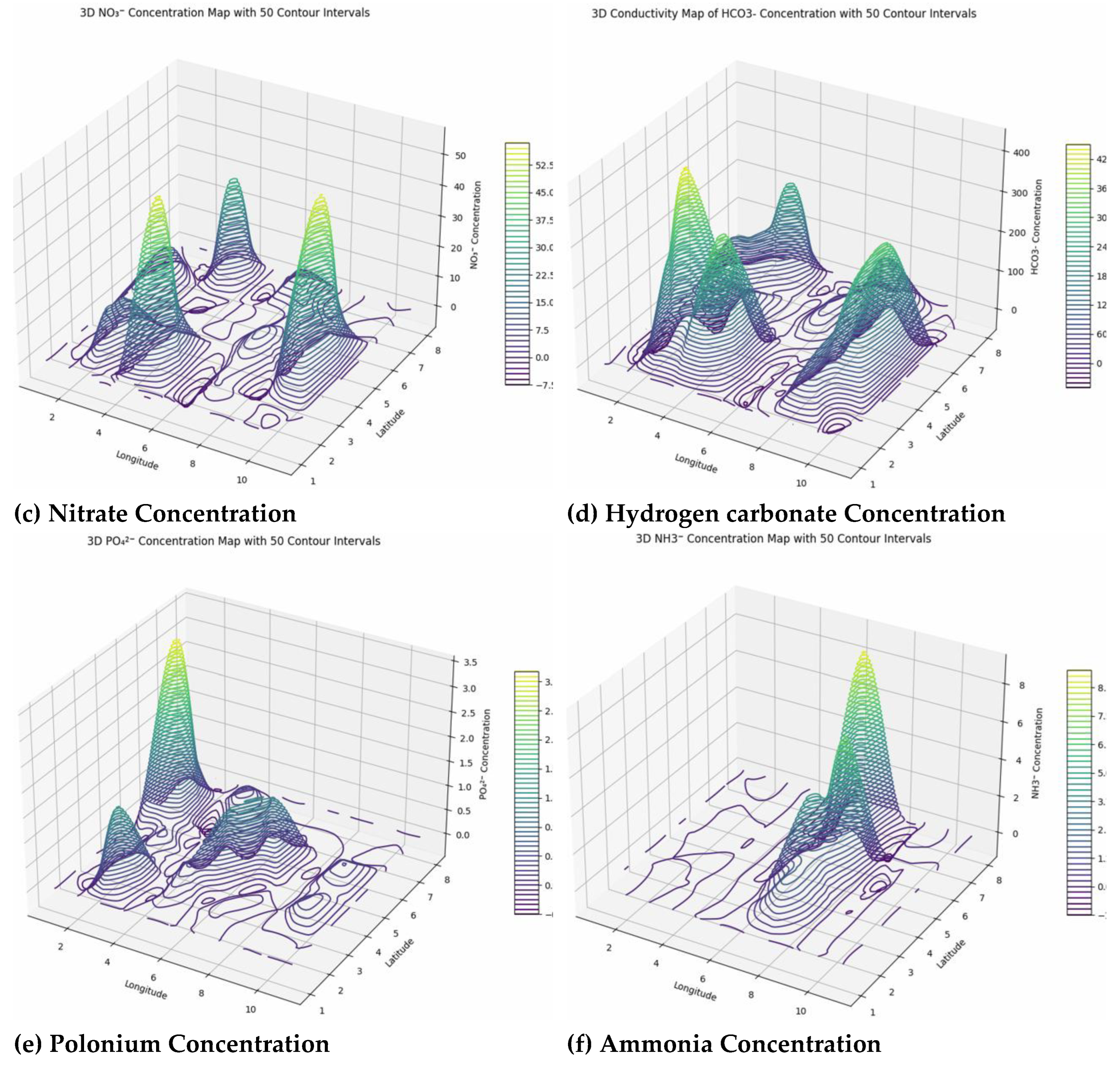
Figure 13.
Scatter plot of the study Area The scatter plot shows that there are strong positive associations between major cations, which are Na+, Mg2+, and Ca2+, indicating that they have geochemical sources like the dissolution of minerals. Zn and Fe are trace elements, and their relationships are more erratic, implying localised effects or contamination in some parts. The separate grouping of the sample points by location is evidence of spatial variation in water chemistry within the regions. On the whole, the plot is convenient for finding out natural hydrochemical patterns and possible outliers to be investigated (Figure 13).
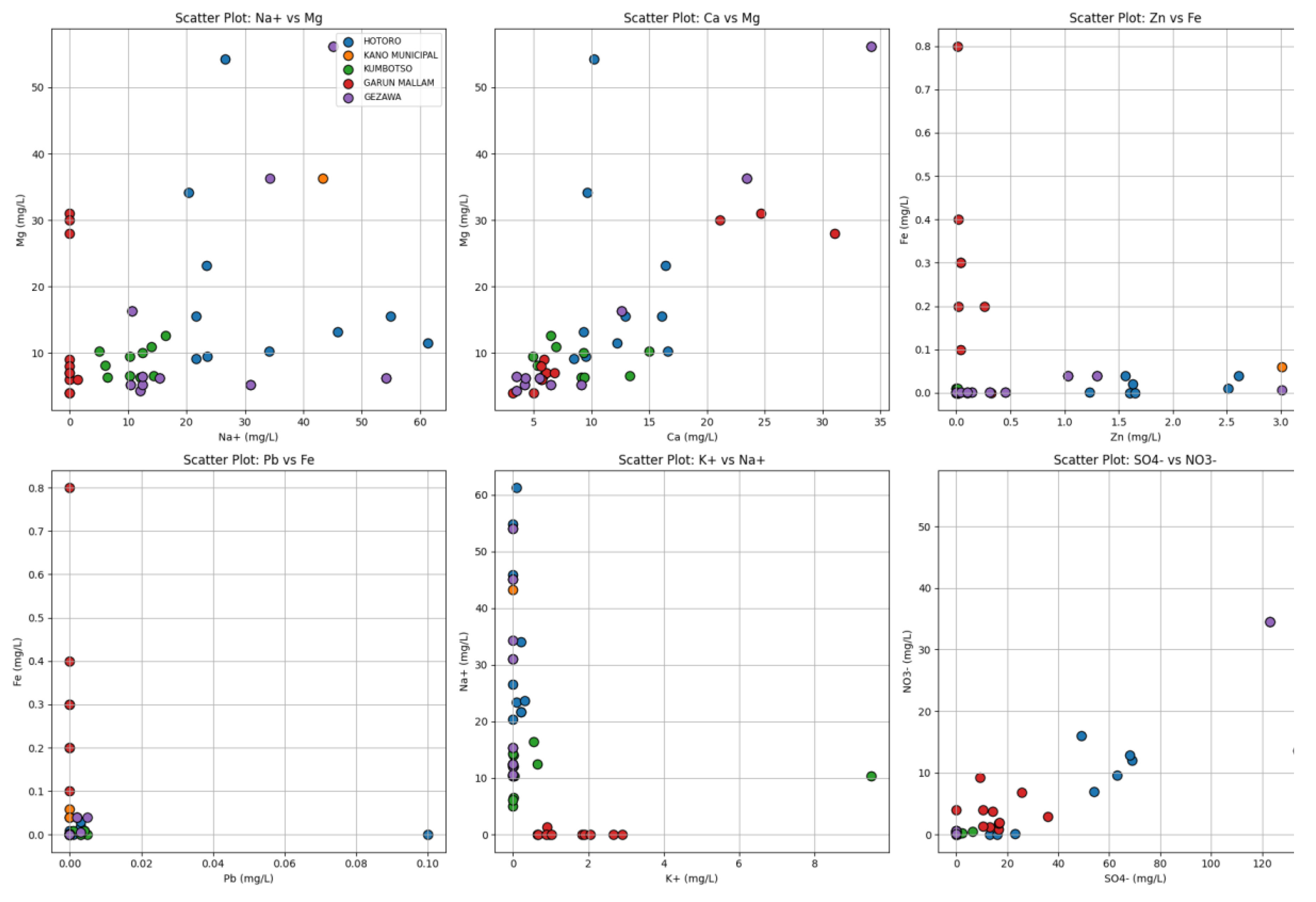
Figure 14.
Principal Component of Curve: The PCA plot shows that most of the variance in the compiled water quality data is explained by the first two principal components, which emphasize the overall patterns of ion concentrations across the entire obsoletely due to the high degree of collinearity between the variables. Distinct hydrochemical patterns and variations across the regional waters are reported by clustering of samples, which represent various geographical clusters. The fact that the groups are separated indicates that there are both natural geological effects involved and potential anthropogenic ones affecting water quality. Generally, PCA provides a good way of distilling the complicated multi-ion data. The PCA plot shows that most of the variance in the compiled water quality data is explained by the first two principal components, which emphasize the overall patterns of ion concentrations across the entire obsoletely due to the high degree of collinearity between the variables. Distinct hydrochemical patterns and variations across the regional waters are reported by clustering of samples, which represent various geographical clusters. The fact that the groups are separated indicates that there are both natural geological effects involved and potential anthropogenic ones affecting water quality. Generally, PCA provides a good way of distilling the complicated multi-ion data.
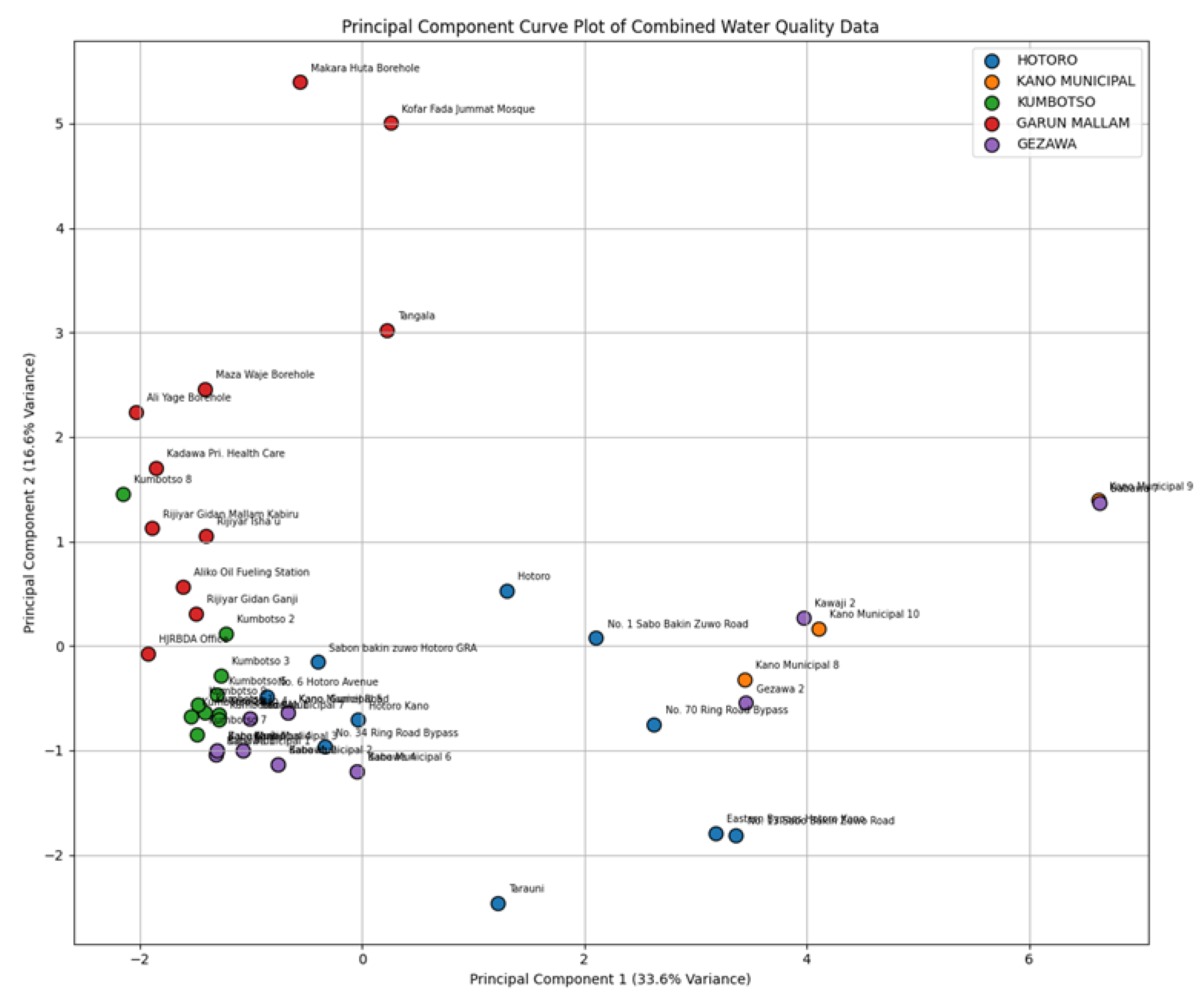
Figure 15.
Piper Trilinear Plot of the Study Area.
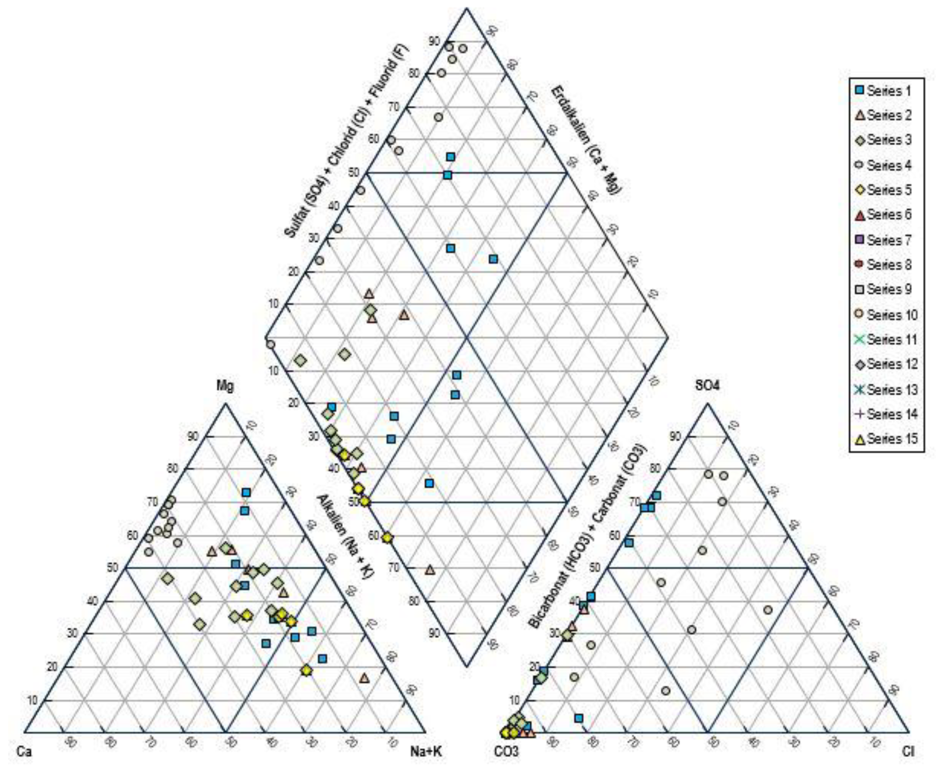
Disclaimer/Publisher’s Note: The statements, opinions and data contained in all publications are solely those of the individual author(s) and contributor(s) and not of MDPI and/or the editor(s). MDPI and/or the editor(s) disclaim responsibility for any injury to people or property resulting from any ideas, methods, instructions or products referred to in the content. |
© 2025 by the authors. Licensee MDPI, Basel, Switzerland. This article is an open access article distributed under the terms and conditions of the Creative Commons Attribution (CC BY) license (http://creativecommons.org/licenses/by/4.0/).
Copyright: This open access article is published under a Creative Commons CC BY 4.0 license, which permit the free download, distribution, and reuse, provided that the author and preprint are cited in any reuse.


