
Submitted:
26 August 2025
Posted:
28 August 2025
You are already at the latest version
Abstract
Proper irrigation scheduling can help to ensure judicial use of water resources, reduce cost of irrigation, and minimize the risks of water management related problems such as waterlogging and salinization. This papers aims to identify the most suitable irrigation scheduling practices for Fincha sugarcane Plantation using modelling and simulation model, CROPWAT, and statistical methods. All data required for modelling and simulation in CROPWAT related to climate, soil, crop, and system parameter were collected and the model was run for irrigation scheduling scenarios formulated using four major irrigation scheduling methods: Fixed, Partially, Mixed Schedule, and On-demand schedule. The model was run for 22 selected scheduling scenarios over replicated over three seasons to simulate performance of irrigation scheduling. The Correlation analysis were carried out to identify the nature of relationship among the performance indicators, analysis of variances (ANOVA) were carried out to check if the irrigation scheduling scenarios have significant effect on irrigation scheduling performance, and multiple least significant difference (MLSD) were carried out to compare the mean values of performance indicators. All the analysis were carried out using R statistical software. It is found that the efficiency of irrigation schedules and efficiency of rainfall are highly correlated while the deficiency and yield reduction are significantly correlated. The ANOVA shows the irrigation scheduling scenarios have significant effect on performance indicators. The MLSD shows on demand scheduling and mixed irrigation scheduling showed highest, equal, and consistent performance for all performance indicators. Considering manageability under existing design, the mixed irrigation scheduling can generally be considered optimal for both soils in Fincha sugar estate. Therefore, it is recommended that the sugar estate shall implement mixed irrigation scheduling practices for optimal yield and water use efficiency.
Keywords:
irrigation scheduling
; performance indicators
; CROPWAT
; correlation
; ANOVA
; MSLD
; Fincha
; Ethiopia
Introduction
Irrigation is the top heavy user of freshwater resources globally. More than 70% the freshwater abstraction from water bodies and 90% of the consumptive use of fresh water is due to irrigated agriculture (FAO, 2015; Grafton, Williams and Jiang, 2017; Zhou et al., 2020). In addition, the demand for irrigation water is increasing associated with the ever increasing demand for food and fiber which in turn are due to growing population and expanding market. On the other hand, the irrigation requirement is also increasing at global scale due to global warming (Grafton, Williams and Jiang, 2017; Zhou et al., 2020; Gabr and Fattouh, 2021; Haile et al., 2024). Furthermore, the amount of fresh water globally available for different uses is becoming more uncertain due to climate change. Under these conditions, improving water management in irrigation systems can greatly contribute in mitigating the global challenges in addition to addressing water management issues locally. Improved irrigation water management is crucial in order to address the global and local water issues.
Improved irrigation water management mainly focuses on saving and conserving water resources. Accordingly, the main focus is reducing the irrigation water needs through different options (Abdelhafid, Gharb and Maarouf, 2022). The improved water management can also be aimed to achieve optimal crop yield, and reduced the risk of water logging and salinization. One of the most important management option in irrigation water management is irrigation scheduling. Irrigation scheduling is the process to determine the amount and frequency of irrigation water application in the field. It can help to reduce the disproportion between water demand and supply, to improve crop yield, reduce risk of water logging and salinization, and there by ensure sustainability of irrigated farms. Irrigation scheduling can optimize crop yield by avoiding under or over irrigation, improve water use efficiency, so saves water and contributes to sustainable water resources management, reduces cost of irrigation especially by avoiding over irrigation, and ensure sustainability of irrigation land by avoiding water logging and salinization problems (Clemmens and Molden, 2007; Etissa et al., 2014; Wabela et al., 2022; Bekele et al., 2024).
In Ethiopia, irrigation development is at nascent stage. More than 85% of total Ethiopian population is heavily dependent on rain feed agriculture. The country is facing frequent and severe devastating droughts despite its huge potential surface and subsurface water resources. Most of the irrigation development in Ethiopia is concentrated in Awash River basin. However, the major surface water resources of the country resides in the Abay (the Blue Nile) River basin.
The basin is the biggest river basin accounting to more than 44% of the surface water resource potential of Ethiopia. The Abay River contributes to more than 62% for the flow of River Nile, the other two rivers add up the remaining share to the total contribution of more than 86 to the flow of Nile. The irrigation potential of the basin is estimated as 815,581 hectares (21.8 % of the total national irrigation potential) (Awulachew et al., 2007; Awlachew, 2010). Yet, there are very few irrigation schemes in Abay River basin. As the result, large majority of rural population in the basin is suffering from lack or absence of irrigation development.
Fincha sugar estate is among the very few irrigation schemes in the Abay basin. The scheme was initiated in 1988 as state farm for production of cereal crops but changed to sugar plantation starting from 1999. The estate uses sprinkler irrigation for its entire sugarcane plantation of around 19,602.6 hectares. The use of such high efficiency irrigation system shows the positive roles the country is playing for improved water management and sustainable use of the Nile water resources. This can be considered exemplary to the downstream countries in the basin, mainly to Egypt which remained reluctant to improve its water resource management and supplement the surface water resources with alternative sources. In Fincha sugar estate, fixed predetermined irrigation schedule was practiced for several years at least until 2002. This schedule consists of the depth and interval of irrigation that are unchanging for all soils, growth stage, and seasons. Accordingly, the sprinkler heads are set at a particular position for 24 hours of operation and returning back to this position at 15 days interval. The operation and maintenance manual by Booker Tate (1998) suggested the use of fixed irrigation schedule only until the irrigation personals get well experienced with operation of the system. The practice could cause over-irrigation for younger growth stages, moisture stress for lighter and shallower soils, especially in dry months and older growth stages, and lower application efficiency for heavy clay soils due to smaller irrigation intervals than required. However, it took several years before the practice was considered for revision. The estate started reconsidering the practice following research recommendation in 2002. The recommendation was to revise the existing fixed schedule and replace it with predetermined irrigation schedule varying with crop stage, soil type, and months of the year (Habib, 2002). The recommendation was based on calculation of irrigation schedules, did not show the impacts on yield and water efficiency. In addition, some schedules are difficult to apply with in the design capability and flexibility of the system and working hours. However, the sugar estate started revising the practice based on subjective assessments.
For instance, the field irrigation interval was increased in black cotton soils. In addition, the estate attempted to vary application depths, trying 12 hours and 6 hours set times. These actions are advantageous in increasing irrigation speed / reduce irrigation period in the given field. This could give more water of required pressure in adjacent and remote fields where irrigation has to go on. However, the estate faced some challenges on applicability of 6 hours set time as it requires night-time shifting of sprinkler positions, making it difficult for field irrigation personnel and field supervisors.
The sugar estate has continued to select and apply more flexible schedule based on subjective assessment. However, the impacts of the revised practices on yield and water efficiency remained unknown. Thus, while it is very impressive to see such progressive adjustment in irrigation scheduling practices under the complex conditions, it is clear that the decisions should be based on empirical evidence of possible impact of irrigation schedules. At least empirical evidence related to the impacts different irrigation schedules on crop yield, and water efficiency need to be made available for the estate be able to make to make informed decision.
The effect of different scheduling scenario are normally evaluated through experimental research under specific local conditions. However, crop models can also provide fairly reliable results with minimal cost and time. It is known that modelling and simulations have great benefit to represent and analyse large number of scenarios in short time and easily which are often costly and difficult to manage even under complex experimental designs. One of the most widely used and effective crop model is CROPWAT (Karuku et al., 2014; Surendran et al., 2015; Kumari, 2017; Moseki, Murray-Hudson and Kashe, 2019; Gabr and Fattouh, 2021; Reta, Hatiye and Finsa, 2024). Local study in Ethiopia shows that CROPWAT is more than 96% efficient in estimation of yield reduction compared with results from field experimentation (Etissa et al., 2014). Another study has recommended use of CROPWAT for irrigation scheduling to achieve more efficient water use and better crop yield at Fincha sugar estate (Geleta, 2019). Therefore, CROPWAT model is used in this study to identify feasible irrigation schedules for sprinkler irrigation system of Fincha sugar estate.
Materials and Methods
The Study Area and Irrgation System
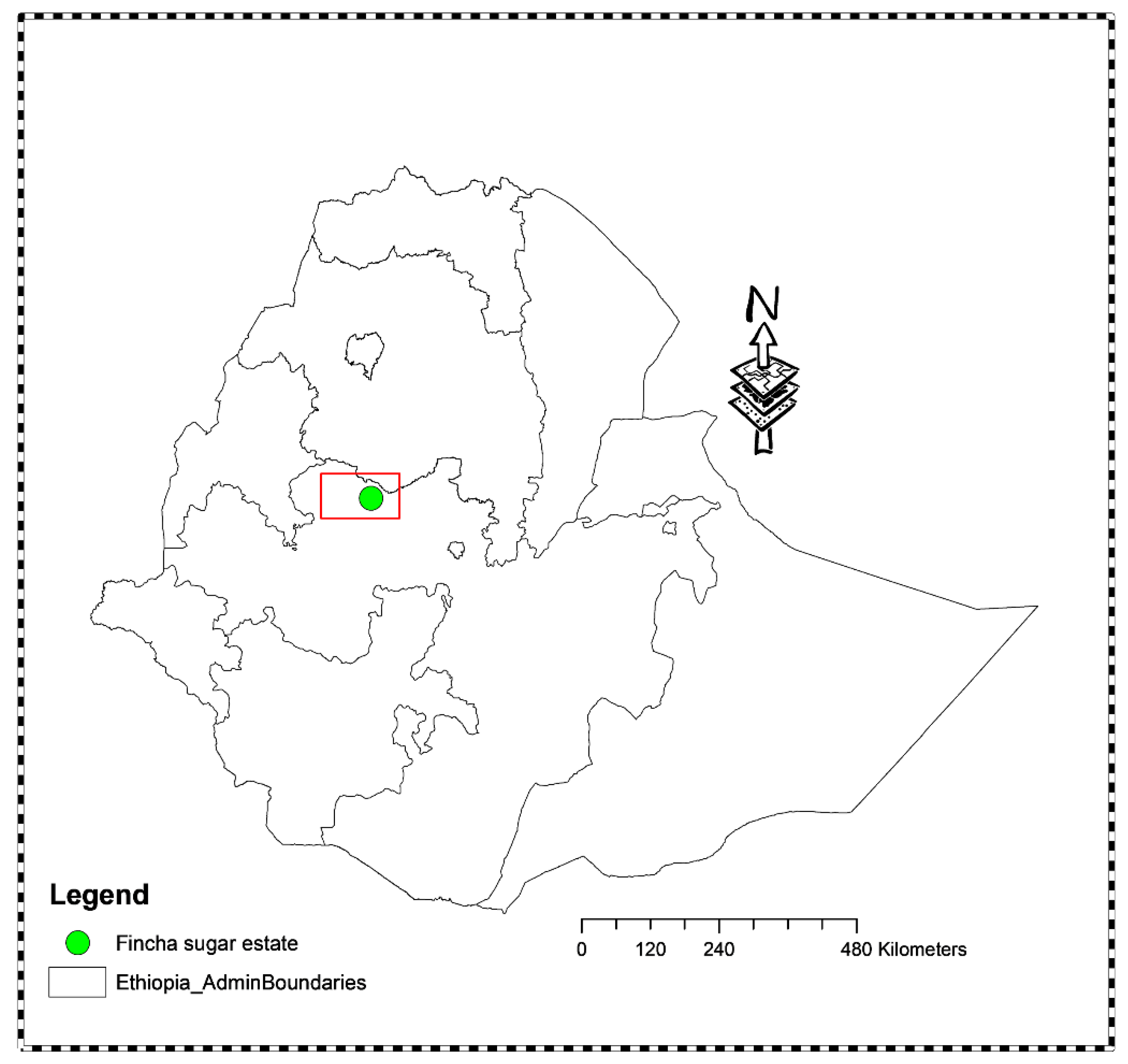
Fincha irrigation scheme is located in 350km west of Addis Ababa in Horo-Gudru Welega zone, Oromia regional state. The source of water for the project is Fincha River, one of the tributaries of the Abay River basin. After the river water is used for hydropower energy generation at Ficha hydropower station, it moves downstream where it is partly diverted and used for sugarcane planation. The sugarcane irrigation scheme is started in 1999 and is among the very few irrigation projects in the basin so far. The irrigation system in Fincha sugar estate is sprinkler irrigation for the entire sugarcane plantation. The sprinkler irrigation system may be the first large scale irrigation project of its kind and among very few irrigation projects in Ethiopia. The scheme was developed in two major phases and one intermediate phases: 6, 200 hectares plantation in the first major phase in the west bank, an expansion and pocket area development of 2,712 hectares in west bank and 400 hectares in East bank, 3,882 hectares in Amerti-Neshi in the intermediate phases, and additional 6,408.8 hectares in East bank in the second major phase. Now, the estate has around 19602 hectares sugarcane plantation.
The existing system is drag-line sprinklers with sprinkler head-tripod setup (design flow rate 5.6mm/hr). Each sprinkler head supplies water to an area of 18 m by 18m (0.0324 hectare) at each setting position. Each sprinkler head-tripod set up has to move to 15 setting positions, five positions across the lateral and two positions along the lateral, to cover the an area of 0.486 hectare. Therefore, a total area of 0.4860 hectare (15*18m*18m) is served by each sprinkler head-tripod setup with in the design irrigation period (15 days) under continuous water supply water, 24 hours per day (Booker Tate, 1998). This means, the system is designed for irrigation water delivery schedule of 24 hours continuous supply to complete irrigating 0.486 hectares in 15 days. The irrigation period is exactly equal to irrigation interval. The particular part of the field (module) can have at least 15 different soil moisture levels.
Figure 1.
Location map of Fincha sugar estate.
Data and Methods
Input Data
All required data related to soil, climate, and crop characteristics, agronomic practices and irrigation system design and management variables were collected from different sources. Soil related information including soil moisture characteristic parameters (soil bulk density, Field capacity (FC), and permanent wilting point (PWP) for two major soils in the study area were obtained from field survey report. The soil of Fincha sugar estate is classified in to two major soils: Luvisols and Vertisols. More than 60% of the planation area is covered by Luviosols and the remaining areas of the sugar estate is covered by Vertisols. The physical properties of these two soils are given in Table 1 and Table 2.
Long years (1994-2019) climatic data including rainfall, temperature, relative humidity, and wind speed required were obtained from the weather station in the sugar estate. Fincha weather station is located at 9.76 oN and 37.42 oE at elevation of 1200m above mean sea level. The summaries of the climatic variable is shown in Table 3.
Information related to crop characteristics (shown Table 4), such as growth stages, periods of the growth stages, rooting depth, and critical water content before wilting were obtained from FAO manuals and previous studies in the area. According to FAO manual, Kc values from FAO tables need to be adjusted for wetting (for Kc ini) and climatic conditions (for Kc mid and end). Accordingly, the Kc ini was estimated as 0.45 corresponding to the average irrigation interval, 15 days, the evaporative Power (ETo), 4.0 mm/day , the amount of irrigation depth > 40mm , and fine and medium texture soils in the area. Similarly, the Kc mid and Kc end values were adjusted for local climate and crop height corresponding to mean daily wind speed of 0.6 m/s , minimum relative humidity of 30.4% , and the crop height of 3m in the area. The adjusted Kc mid and Kc end were 1.252 and 0.7524, respectively. The adjusted values are only slightly different from Kc values from tables, Kc mid= 1.25 and Kc end =0.75.
The existing agronomic practices in the sugar estate were also considered to identify the planting season and harvest age. Under existing cultural practices, February, March, and April are suitable planning months. Harvest age is typically around 24 months for plant cane and around 12 months for ratoon crops. Lastly, information regarding the design and management variables were obtained from operation and maintenance manuals. The information related to flow (rate, duration, and frequency of flow), design operating pressure, irrigation scheduling practice, and application efficiency were obtained. It is noted that the design operating pressure in lateral is 5 bar, sprinkler flow rate is 5.6 mm per hour, and application efficiency is 75%. The field water delivery capacity of a single sprinkler head is characterized by flow rate of 5.6 mm per hour operating 24 hours per day to irrigate 0.468 hectares within 15 days.
Alternative Irrigation Scheduling Scenarios
Four major methods for scheduling methods were considered. These methods included are fixed pre-determined Scheduling, Partially flexible pre-determined scheduling, mixed scheduling, and on- demand irrigation scheduling methods. The scheduling methods and irrigation scheduling scenarios considered for investigation are described below.
- A)
- Fixed pre-determined Schedule
Predetermined rigid schedules are followed over the growth stage and seasons. Two options are included
- ➢
- Design schedule: Depth: 24 hours set time and interval: 15 days is used for all soils for all times
- ➢
- Modified fixed schedule: the design schedule was modified for each soil class based on soil, crop, and system parameters.
Accordingly, the following fixed predetermined schedules were selected as alternatives
For Luvisol
- ➢
- Depth: 24 set time (101mm) and interval: 15 days intervals, Luvisols (scenario 1a)
- ➢
- Depth: 16 set time (67mm) and interval: 12 days intervals Luvisols (scenario 2a)
- ➢
- Depth: 12 set time (50mm) and interval: 10 days intervals, Luvisols (scenario 3a)
- ➢
- Depth: 12 set time (50mm) and interval: 8 days intervals, Luvisols (scenario 4a)
For Vertisol
- ➢
- Depth: 24 set time (101mm) and interval: 15 days intervals, Vertisol (scenario 1b)
- ➢
- Depth: 16 set time (67mm) and interval: 15 days intervals, Vertisol (Scenario 2b)
- ➢
- Depth: 12 set time (50mm) and interval: 15 days intervals, Vertisol (Scenario 3b)
- ➢
- Depth: 12 set time (50mm) and interval: 10 days intervals, Vertisol (Scenario 4b)
- B)
- Partially flexible pre-determined schedule
Partially flexible predetermined schedules consisting of depth and interval varying across growth stages for each soil type were considered. The values of depth and intervals were calculated based on soil, crop, and system parameters. For each soil, 4 application depths and 4 irrigation intervals are combined to form a total 16 irrigation scheduling scenarios (Table 5 and Table 7). Table 6 and Table 8 show the net application depths (in mm) for two soil types corresponding to Table 5 and Table 7, respectively.

Table 5.
Irrigation scheduling scenarios for Luvisol.
| Scenarios | Set time in hours/Irrigation intervals in days over stages | ||||
| Initial stage | Crop devlop | Mid-season | Late & harvest | ||
| codes | D1 | 6 | 8 | 12 | 12 |
| 5 a | I1 | 9 | 9 | 10 | 16 |
| 6a | I2 | 10 | 10 | 12 | 18 |
| 7a | I3 | 12 | 12 | 14 | 20 |
| 8 a | I4 | 4 | 5 | 8 | 8 |
| D2 | 6 | 10 | 12 | 12 | |
| 9a | I1 | 9 | 9 | 10 | 16 |
| 10a | I2 | 10 | 10 | 12 | 18 |
| 11a | I3 | 12 | 12 | 14 | 20 |
| 12a | I4 | 4 | 6 | 8 | 8 |
| D3 | 6 | 12 | 12 | 12 | |
| 13a | I1 | 9 | 9 | 10 | 16 |
| 14a | I2 | 10 | 10 | 12 | 18 |
| 15a | I3 | 12 | 12 | 14 | 20 |
| 16a | I4 | 4 | 8 | 8 | 8 |
| D4 | 12 | 12 | 12 | 12 | |
| 17a | I1 | 9 | 9 | 10 | 16 |
| 18a | I2 | 10 | 10 | 12 | 18 |
| 19a | I3 | 12 | 12 | 14 | 20 |
| 20a | I4 | 8 | 8 | 8 | 8 |
Table 6.
Net application depths (in mm) for Luvisol.
| Depths (mm) | Initial stage | Crop devlop. | Mid-season | Late & harvest |
| D1 | 25.2 | 33.6 | 50.4 | 50.4 |
| D2 | 25.2 | 42 | 50.4 | 50.4 |
| D3 | 25.2 | 50.4 | 50.4 | 50.4 |
| D4 | 50.4 | 50.4 | 50.4 | 50.4 |
Table 7.
Irrigation scheduling scenarios for Vertisol.
| Scenarios | Set time in hours/Irrigation intervals in days over stages | ||||
| Initial stage | Crop devlop. | Mid-season | Late & harvest | ||
| codes | D1 | 12 | 12 | 24 | 24 |
| 5 b | I1 | 18 | 18 | 20 | 26 |
| 6b | I2 | 20 | 20 | 20 | 28 |
| 7b | I3 | 22 | 22 | 22 | 28 |
| 8 b | I4 | 8 | 8 | 15 | 15 |
| D2 | 12 | 16 | 24 | 24 | |
| 9b | I1 | 18 | 18 | 20 | 26 |
| 10b | I2 | 20 | 20 | 20 | 28 |
| 11b | I3 | 22 | 22 | 22 | 28 |
| 12b | I4 | 8 | 10 | 15 | 15 |
| D3 | 12 | 20 | 24 | 24 | |
| 13b | I1 | 18 | 18 | 20 | 26 |
| 14b | I2 | 20 | 20 | 20 | 28 |
| 15b | I3 | 22 | 22 | 22 | 28 |
| 16b | I4 | 8 | 13 | 15 | 15 |
| D4 | 12 | 24 | 24 | 24 | |
| 17b | I1 | 18 | 18 | 20 | 26 |
| 18b | I2 | 20 | 20 | 20 | 28 |
| 19b | I3 | 22 | 22 | 22 | 28 |
| 20b | I4 | 8 | 15 | 15 | 15 |
Table 8.
Net application depths (in mm) for Vertisol.
| Depths (mm) | Initial stage | Crop devlop. | Mid-season | Late & harvest |
| D1 | 50.4 | 50.4 | 100.8 | 100.8 |
| D2 | 50.4 | 67.2 | 100.8 | 100.8 |
| D3 | 50.4 | 84 | 100.8 | 100.8 |
| D4 | 50.4 | 100.8 | 100.8 | 100.8 |
- C)
- Mixed Schedule
Mixed schedule consists of pre-determined irrigation depth varying with growth stage and irrigation intervals that depend on selected level of optimal soil moisture deficit before irrigation. The values of depth of application are calculated based on soil, crop, and system parameters. Accordingly, depth of irrigation varying with growth stage shown in Table 10 are applied at irrigation interval corresponding to critical depletion (65%) for two soil types. This method is compatible with the existing system but soil moisture monitoring practice is needed. Thus, it is included to explore and assess alternative practice for improvement.
Table 9.
Net application depths (mm (hours)).
| Net Depths | Initial stage | Crop devlop. | Mid-season | Late & harvest | Soil |
| D1 |
34 (8) | 59(14) | 67(16) | 100(24) | Luvisol |
| D2 |
75(18) | 100(24) | 100(24) | 100(24) | Vertisol |
- ➢
- Depth: D1 and interval: 65% depletion , Luvisols (scenario 21a)
- ➢
- Depth: D2 and interval: 65% depletion , Vertisol (scenario 21b)
- D)
- On-demand schedule
Both depth and interval are fully flexible schedule. The delivery is based on soil moisture deficit at selected level of depletion. Neither the depth nor intervals are predetermined and fixed. Accordingly, irrigation water is applied when critical soil moisture depletion (65% depletion) is reached to refill the root zone to field capacity. This method is difficult to apply under existing the system due to high flexibility needed and operational complexity. Yet, this method is included as a reference to compare the result s with other methods.
As it can be noted above a number of alternative scheduling options employing four different major scheduling methods were identified. This is done in order to evaluate large number of possible alternatives of irrigation scheduling. All alternatives except on- demand irrigation scheduling alterative are with in operational flexibility limits of the systems. The on- demand irrigation scheduling alterative is included as reference or control to compare the results with other methods. This scenario is ideal, cannot be applied in field due to complexity for field application.
Modeling and Simulation Analysis
All the input data were organized and used in the CROPWAT software. The effective rainfall was estimated using USDA Soil Conservation Method. The initial soil moisture depletion as percentage of total available water were considered as 50 % for both Luvisols and Vertisols to account for soil moisture withdrawals after pre-irrigation water application events. Pre-irrigation water application practices are common in sugarcane fields.
They are carried out before normal irrigation season for the purpose of initiating germination and regulation of soil temperature for germination and tillering. Irrigation scheduling options suitable for each of irrigation scheduling scenarios were set in the CROPWAT model. For predetermined irrigation scheduling methods (A and B), the scheduling option was set for user’s defined depth and intervals. For mixed scheduling method (C), the scheduling option was set for user’s defined depth of irrigation varying with growth stage and irrigation timing corresponding to 100% of the selected critical depletion level. For fully flexible irrigation scenario (D), the scheduling option was set for irrigation timing corresponding to 100% of the selected critical depletion level and depth of irrigation to refill the root zone to field capacity. The modelling and simulation analysis were run for a total of 132 times (for two soil types, for 22 irrigation scheduling scenario each replicated three times corresponding to three typical planting dates in the planting seasons). The simulated scheduling performance indicators used in this study include: efficiency irrigation schedule, deficiency irrigation schedule, and efficiency rain yield reduction.
Statistical Analysis
Correlation analysis was performed to identify the relationships among the various irrigation scheduling performance indicators. Analysis of variance (ANOVA) was carried out to check out the whether the different irrigation scheduling scenarios have statistically significant effect on scheduling performance. The ANOVA was carried out using a randomized complete block design (RCBD) with 22 levels of irrigation scheduling scenarios, each replicated three times (three planting dates). When significant effects on scheduling performance were detected, the mean values of the performance indicators were compared by multiple comparisons of means based on least significant difference (LSD). All statistical analysis were performed using R 4.2.3 - statistical software , employing some basic and special packages analysis and plotting packages such as ggplot2, ggpubr, tidyverse, broom, AICcmodavg, Tidyverse, and Agricolae.
Results and Discussions
Correlation Analysis
The correlation analysis matrix (Table 10) and Multiple scatterplots (Figure 2 and Figure 3) for scheduling performance indicators show that there is strong statistically significant positive correlation between efficiency of scheduling (EIS) and rainfall efficiency (RE) (0.8 for Luvisoil and 0.86 for Vertisol). Similarly, there is very strong statistically significant positive correlation between deficiency of irrigation schedule (DIS) and yield reduction (YR) (0.99 for both Luvisoil and Vertisol). These results are in line with the inherent nature of the indicators. However, all other relationships are not statistically significant. Based on correlation analysis, the performance indicators can be grouped in to two: as efficiency related (efficiency of irrigation schedule and efficiency of rainfall) and yield related indicators (deficiency of irrigation schedule and yield reduction). This categorization of the performance indicators can help to simplify the selection of optimal irrigation scheduling scenario.
Table 10.
Correlation matrix (Luvisol and Vertisol).
| Luvisol | Vertisol | ||||||||
| EIS | DIS | ER | YR | EIS | DIS | ER | YR | ||
| EIS | 1 | 0.19 | 0.80 | 0.19 | EIS | 1 | 0.07 | 0.86 | 0.07 |
| DIS | 1 | 0.34 | 1.00 | DIS | 1 | 0.27 | 1.00 | ||
| ER | 1 | 0.342 | ER | 1 | 0.27 | ||||
| YR | 1 | YR | 1 | ||||||
Note EIS- efficiency of irrigation schedule, DIS- Deficiency of irrigation schedule, ER- efficiency of rain, and YR- yield reduction.
Analysis of Variance (ANOVA)
For Luvisol , the summary of the analysis of variance (ANOVA) for the different indicators given in Table 11, Table 12, Table 13 and Table 14 show that irrigation scheduling scenarios have very high statistically significant (at α< 0.001) effect on scheduling performance. The replications (planting dates) have also showed very high statistically significant (at α< 0.001) effect on scheduling performance. This indicates planting seasons affect water application performance and final yield. Looking at the plots of scheduling performance indicators for the different scheduling scenarios over the three planting seasons (Appendix A Figure A1, Figure A2, Figure A3 and Figure A4), efficiency related performance indicators for planting in February are consistently better than that of March and April. In contrast, yield related performance indicators for planting in April are consistently better than that of March and February. The coefficient of variation (CV) for different indicators is generally very low (varying from 3.1 to 14.5 %), indicating that the data set and the statistical design used are highly reliable.
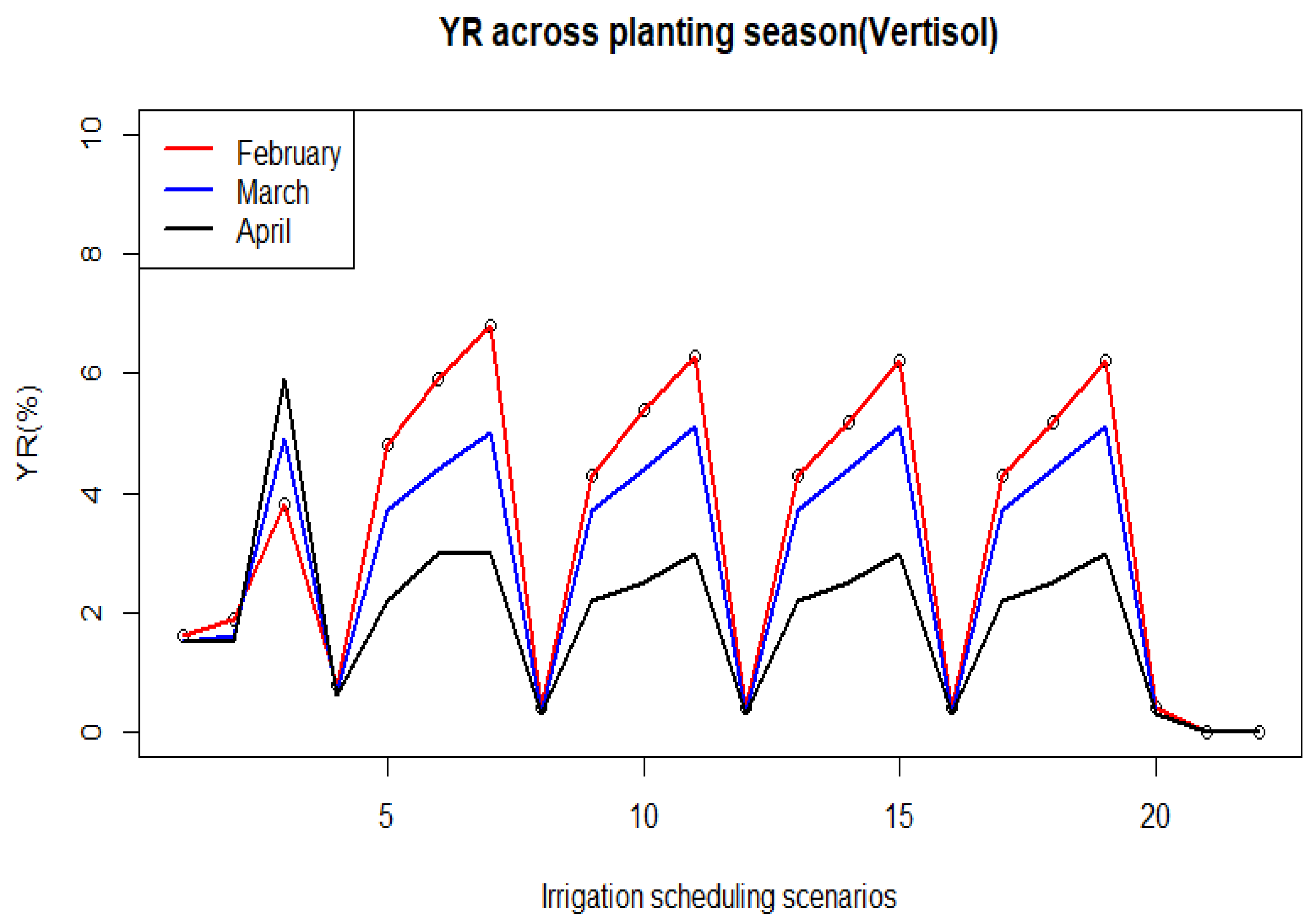
For Vertisols, the summary of the analysis of variance (ANOVA) for the different indicators shown in Table 15, Table 16, Table 17 and Table 18 show that irrigation scheduling scenarios have very high statistically significant (at α< 0.001) effect on scheduling performance. The replications (planting seasons) have also showed very high statistically significant (at α< 0.001) effect on scheduling performance. This indicates planting seasons affect water application performance and final yield. Looking at the plots of scheduling performance indicators for the different scheduling scenarios over the three planting seasons (Appendix A, Figure A5, Figure A6, Figure A7 and Figure A8), efficiency related performance indicators for planting in February are consistently better than that of March and April. In contrast, yield related performance indicators for planting in April are consistently better than that of March and February. The coefficient of variation (CV) for different indicators is generally very low (varying from 3.1 to 14.5 %), indicating that the data set and the statistical design are highly reliable.
Mean Comparison for Simulated Scheduling Performance
The mean values for the simulated scheduling performance for each indicator corresponding to each scheduling scenario are shown in the Appendix A, Table A1 and Table A2. Owing to the fact that irrigation scheduling scenarios showed statistically significant effects on scheduling performance, the mean separation analysis were carried out using Multiple LSD. The results of mean separation for Luvisol and Vertisols are shown in Table 19 and Table 20, respectively.
Mean Comparison for Simulated Scheduling Performance in Luvisols
In Luvisol (Table 19), the irrigation scheduling scenarios can be grouped in to 16 groups based on their effect on the efficiency of irrigation schedule. The top four best performing groups include: group a (22a), group b (21a), group c (7a), and group cd (6a, 11a, and 10a). Accordingly, the highest efficiency of irrigation schedule is achieved for on- demand scheduling (22a) followed by that of mixed scheduling (21a). The third and fourth best performance are found for partially flexible pre-determined schedules, scenario 7a and scenarios (6a, 11a, 10a), respectively. The least efficiency of irrigation schedule is achieved at fixed predetermined irrigation scheduling (1a) followed by that of some fixed predetermined irrigation scheduling (2a and 4a) and a partially flexible pre-determined schedule (8a).
Based on their effect on deficiency of irrigation schedule, the irrigation scheduling scenarios can be grouped in to 11 groups for Luvisol , the top four best performing groups include: group h (22a, 21a, 12a, 16a), group gh (20a, 4a, 3a, 2a, 1a), group fg (1a, 17a), and group ef (5, 13). These schedules consists of schedules on- demand (22a), mixed schedule (21a), and some partially flexible pre-determined schedules (12a, 16a, 17a, 20a), and fixed predetermined schedules (1a, 2a, 3a, 4a). The least performing four groups include: group a (15a and 11a), group ab (7a), group b (19a), and group c (10a, and 14a). It can be noted, the irrigation schedule corresponding to these least performing groups are all partially flexible pre-determined schedules (15a, 11a, 7a, 19a, 10a, and 14a).
Based on their effect on the efficiency of rainfall, the irrigation scheduling scenarios can be grouped in to 7 groups for Luvisol , the top four best performing groups include: group a (22a, 21a), group b (7a, 11a, 15a), group bc (9a, 19a, and 1a), and group bcd (6a,10a, 14a, 5a, 13a, 18a, 17a). These schedules consists of schedules on- demand (22a), mixed schedule (21a), and some partially flexible pre-determined schedules (7a, 11a, 15a, 9a, 19a, 6a, 10a, 14a, 5a, 13a, 18a, 17a), and fixed predetermined schedules (1a). The least performing three groups include: group cd (2a), group d (3a), group e (20a, 4a, 16a, 12a, and 8a). It can be noted, the irrigation schedule corresponding to these least performing groups are all partially flexible pre-determined schedules.
Based on their effect on the on percentage yield reduction, the irrigation scheduling scenarios can be grouped in to 11 groups for Luvisol , the top four best performing groups include: group h (22a, 21a,12a, 16a, 8a), group gh (20a, 4a,3a, 2a), group fg (1a, 17a), and group ef (5a, and 13a). Accordingly, the highest yield is achieved for on- demand scheduling (22a), mixed scheduling (21a), and some partially flexible irrigation schedule (12a, 16a, 8a). The least performing three groups include: group c (10a and 14a), group b (19a), group ab (7a), and group a (14a and 15a). The least yield is achieved at partially flexible predetermined irrigation scheduling.
Mean Comparison of Simulated Scheduling Performance in Veritisols
In Vertisol (Table 20), the irrigation scheduling scenarios can be grouped in to 10 groups with respect to their effect on efficiency of irrigation schedule. The top four best performing groups include: group a (22b and 21b), group b (3b), group cd (11b, 6b), and group cde (15b). Accordingly, the highest efficiency of irrigation schedule is achieved for on- demand scheduling (22a) and the mixed scheduling (21a), followed by some partially flexible pre-determined schedules (3b, 11b, 6b, 15b). The least efficiency of irrigation schedule is achieved at partially flexible pre-determined schedule (8b,) followed by that of a fixed schedule (1b) and another partially flexible pre-determined schedule (12b). Some other partially flexible pre-determined schedule (12b, and 16b, 20b) show the next least performance.
Based on their effect on deficiency of irrigation schedule, the irrigation scheduling scenarios can be grouped in to 4 groups for Verisol , the two best performing groups include: group c (22b, 21b, 12b, 16b, 20b, 8b, and 4b) and group bc (1b and 2b). These schedules consists of schedules on- demand (22b), mixed schedule (21b), some partially flexible pre-determined schedules (12b, 16b, 20b, 8b), and a fixed predetermined schedule (1b, 2b). The least performing two groups include: group ab (13b, 17b, 9b, 5b, 14b, 18b, and 10b), and group a (6b, 15b, 19b, 11b, 3b, and 7b). It can be noted, the irrigation schedule corresponding to these least performing groups are all partially flexible pre-determined schedules.
Based on their effect on the efficiency of rainfall, the irrigation scheduling scenarios can be grouped in to 11 groups for Vertisol. The top four best performing groups include: group a (22b, 21b), group b (6b and 7b), group bc (10b), and group bcd (3b, 5b, 11b, 14b and 18b). These schedules consists of schedules on- demand (22b), mixed schedule (21b), and some partially flexible pre-determined schedules (5b, 6b, 7b, 11b, 14b and 18b), and fixed predetermined schedules (3b).
The least performing four groups include: group fghi (1b), group ghi (12b, 20b, 16b), group hi (8b) and group i (4b). It can be noted, the irrigation schedule corresponding to these least performing groups are all partially flexible pre-determined schedules.
Based on their effect on the on percentage yield reduction, the irrigation scheduling scenarios can be grouped in to 4 groups for Vertisol , the top two best performing groups include: group c (22b, 21b, 12b, 16b, 20b, 8b, and 4b) and group bc (1b and 2b). Accordingly, the highest yield is achieved for on- demand scheduling (22a), mixed scheduling (21a), some partially flexible irrigation schedule (12b, 16b, 20b, and 8b), and a fixed schedule (4b). The fixed predetermined irrigation schedule (1b and 2b) shows the next best performance. The least performing three groups include: group ab (13b, 17b, 9b, 5b, 14b, 18b, and 10b), and group a (3b, 6b, 7b, 11b, 15b, and 19b). It can be noted, the irrigation schedule corresponding to these least performing groups are all partially flexible pre-determined schedules.
Summary
Summarizing the results, based on results from correlation analysis, analysis of variance, and mean separation, it can be noted that there is strong correlation and symmetrical pattern between efficiency irrigation schedule and rainfall efficiency. Similarly, there is strong correlation and symmetrical pattern between deficiency irrigation scheduling and yield reduction efficiency. It is also noted that yield related factors are contrasted by efficiency related indicators for all irrigation scheduling scenarios, except on-demand and mixed scheduling scenarios. For instance, for irrigation scheduling scenarios 7b, least yield related performance is achieved while the efficiency related performance is higher in both soils.
The irrigation scheduling scenarios 22 (on demand scheduling) and the irrigation scheduling scenarios 21 (Mixed scheduling) are the top two best performing ones. For all performance indicators and for both soils, the irrigation scheduling scenarios 22 (on demand scheduling) has showed best performance, followed by the irrigation scheduling scenarios 21 (Mixed scheduling). In addition, only these two irrigation scheduling scenarios have consistently showed similar performance for all performance indicators. These conditions indicate the two scenarios meet ideal condition for irrigation water management in achieving both high efficiency and high yield. However, it is already known that there are some practical limitations to the on-demand scheduling alterative, as it requires very high flexibility that cannot be achieved under existing design and operation management. The other option, which is equally performing with that of on-demand schedule, is the mixed irrigation scheduling. This can be applied in the sugar estate by introducing soil moisture monitoring practice.
The soil samples for soil moisture monitoring shall be taken at spots irrigated at first sprinkler-tripod setting for each module area. However, until such practices are going to be implemented, the sugar estate can select and use scheduling scenario depending on the particular situation. Under existing normal condition where maximum yield is an issue than water scarcity. Thus, irrigation scheduling scenarios with zero yield reductions such as irrigation scheduling scenarios (16a, and 8a) in Luvisol and irrigation scheduling scenarios (4b, 16b, 20b, and 12b, shown in order of priority) in Vertisol can be considered as second option. However, when water scarcity comes to be the issue such as due to drought conditions, scheduling scenarios achieving high efficiency from the list can be selected and applied by accepting some decline in yield. The results also shows that among the three planting months, February, March, and April, yield reduction is lowest in April and efficiency is lowest in February. That means earlier planning appears more desirable when water efficiency is the main issue while late planting is desirable when yield is the main issue.
Studies show that the sugarcane yield and water use efficiency heavily rely on irrigation scheduling at various physiological growth stages (Khan, 2021). A number of studies estimated the optimal irrigation schedules for different crops using CROPWAT(Kumari, 2017; Balasaheb and Biswal, 2020; Wabela et al., 2022; Soomro et al., 2023). However, there are no similar studies locally to compare the results with.
Conclusions and Recommendations
On demand and mixed irrigation scheduling methods showed highest, equal, and consistent performance for all performance indicators. The performance of the on-demand schedule is found similar with that of mixed schedule. On-demand schedule is not manageable under the existing design and management practices of the sprinkler system at Fincha sugar estate. This is because such flexibly requires estimation of soil moisture deficit in root zone before irrigation and replace the same amount of water in to the soil during each irrigation event. It is clear that there is no advantage to apply fully flexible schedule in the sugar estate. Therefore, mixed irrigation scheduling (21a) can generally be considered optimal for both soils in Fincha sugar estate. However, in very near future, the mixed schedule may not be applied due to absence of soil monitoring practice in the sugar estate. Additionally, the need to stop and start water supply to fields to wait for proper soil moisture deficit under mixed scheduling option may require very close supervision and effective communication in irrigation system operation. Therefore, the sugar estate shall start working to implement mixed irrigation scheduling practices. But until, then other alternatives irrigation scheduling scenarios that can achieve next better combination of efficiency and yield performance shall be selected from the ranked list of alternatives scheduling scenarios in Table 19 and Table 20. Accordingly, use of irrigation scheduling scenarios (8a and 16a) for Luvisol and irrigation scheduling scenarios (4b, 16b, 20b, and 12b) for Vertisol are recommended for the immediate application under normal conditions. However, if water scarcity comes to be the issue such as due to drought conditions, scheduling scenarios achieving high efficiency from the list shall selected and applied by accepting some level of decline in yield. This study has not only identified the suitable irrigation schedule, but also provides important insight on effect of planting season on yield and water use efficiency. Thus, the estate shall use the information for decision making regarding planting seasons based on desired performance in the particular time and conditions.
Funding
No government or private funding support was available to this research.
Conflicts of Interest
There is no conflict of interest with regard to publication of this research manuscript
Appendix A
Table A1.
Mean simulated application performances and yield losses for Luvisol.
| Scenarios | Efficiency irrigation schedule | Deficiency irrigation schedule | Efficiency rain | Yield reduction (%) |
| 1b | 39.1 | 2.5 | 51.4 | 2.9 |
| 2b | 49.5 | 1.8 | 48.2 | 2.1 |
| 3b | 56.7 | 1.2 | 46.4 | 1.4 |
| 4b | 48.9 | 0.7 | 40.7 | 0.9 |
| 5 b | 63.4 | 3.9 | 50.2 | 4.7 |
| 6b | 69.8 | 6.9 | 50.8 | 8.3 |
| 7b | 70.3 | 11.4 | 53.5 | 13.7 |
| 8 b | 48.4 | 0.1 | 36.5 | 0.1 |
| 9b | 60.9 | 5.1 | 52.5 | 6.1 |
| 10b | 68.1 | 7.2 | 50.6 | 8.7 |
| 11b | 68.4 | 11.8 | 53.3 | 14.2 |
| 12b | 56.3 | 0.1 | 39.3 | 0.1 |
| 13b | 60.0 | 4.2 | 49.7 | 5.1 |
| 14b | 66.0 | 7.2 | 50.4 | 8.7 |
| 15b | 66.5 | 11.8 | 53.0 | 14.1 |
| 16b | 53.5 | 0.1 | 40.3 | 0.1 |
| 17b | 58.8 | 2.6 | 48.9 | 3.1 |
| 18b | 64.8 | 5.3 | 49.4 | 6.3 |
| 19b | 66.4 | 9.5 | 52.2 | 11.4 |
| 20b | 51.2 | 0.7 | 40.7 | 0.9 |
| 21b | 90.9 | 0.0 | 61.7 | 0.0 |
| 22b | 100.0 | 0.0 | 64.7 | 0.0 |
Table A2.
Mean simulated application performances and yield losses for Vertisol.
| Scenario | Efficiency irrigation schedule | Deficiency irrigation schedule | Efficiency rain | Yield reduction |
| 1a | 42.0 | 1.3 | 51.6 | 1.5 |
| 2a | 61.9 | 1.3 | 52.3 | 1.7 |
| 3a | 73.2 | 4.1 | 57.4 | 4.9 |
| 4a | 58.9 | 0.6 | 47.3 | 0.7 |
| 5 a | 62.3 | 3.0 | 56.8 | 3.6 |
| 6a | 64.0 | 3.7 | 59.7 | 4.4 |
| 7a | 66.7 | 4.1 | 60.4 | 4.9 |
| 8 a | 38.6 | 0.3 | 49.8 | 0.3 |
| 9a | 61.0 | 2.9 | 56.0 | 3.4 |
| 10a | 60.8 | 3.4 | 58.9 | 4.1 |
| 11a | 64.3 | 4.0 | 56.9 | 4.8 |
| 12a | 42.1 | 0.3 | 51.2 | 0.3 |
| 13a | 60.1 | 2.8 | 54.5 | 3.4 |
| 14a | 60.0 | 3.3 | 57.5 | 4.0 |
| 15a | 62.9 | 4.0 | 56.5 | 4.8 |
| 16a | 43.4 | 0.3 | 50.2 | 0.3 |
| 17a | 58.6 | 2.8 | 54.1 | 3.4 |
| 18a | 58.1 | 3.3 | 57.5 | 4.0 |
| 19a | 61.3 | 4.0 | 56.5 | 4.8 |
| 20a | 43.3 | 0.3 | 50.5 | 0.3 |
| 21a | 100.0 | 0.0 | 65.0 | 0.0 |
| 22a | 100.0 | 0.0 | 67.6 | 0.0 |
Figure A1.
Efficiency irrigation schedule over planting seasons (Luvisol).
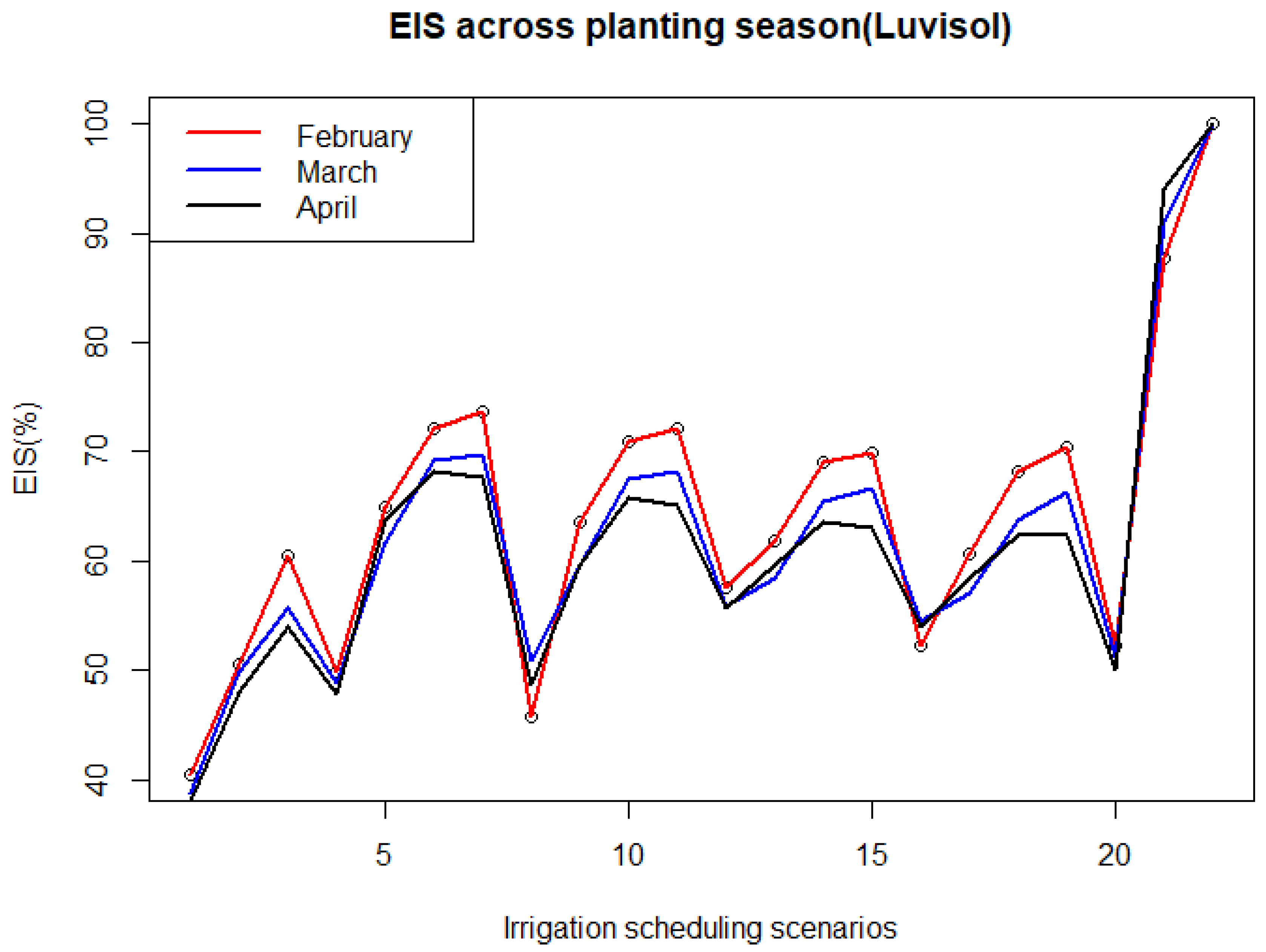
Figure A2.
Deficiency irrigation schedule over planting seasons (Luvisol).
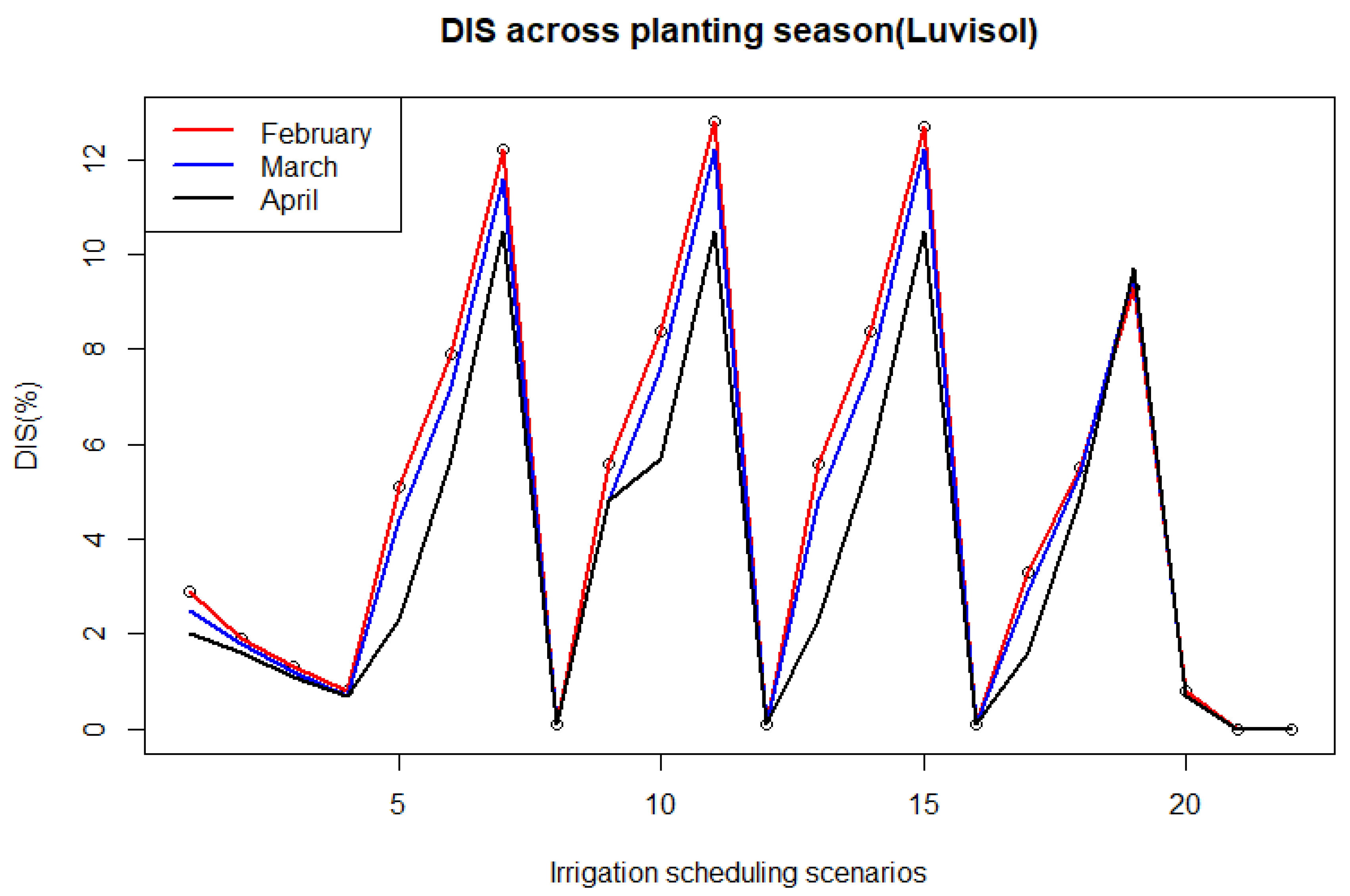
Figure A3.
Efficiency of rain over planting seasons (Luvisol).
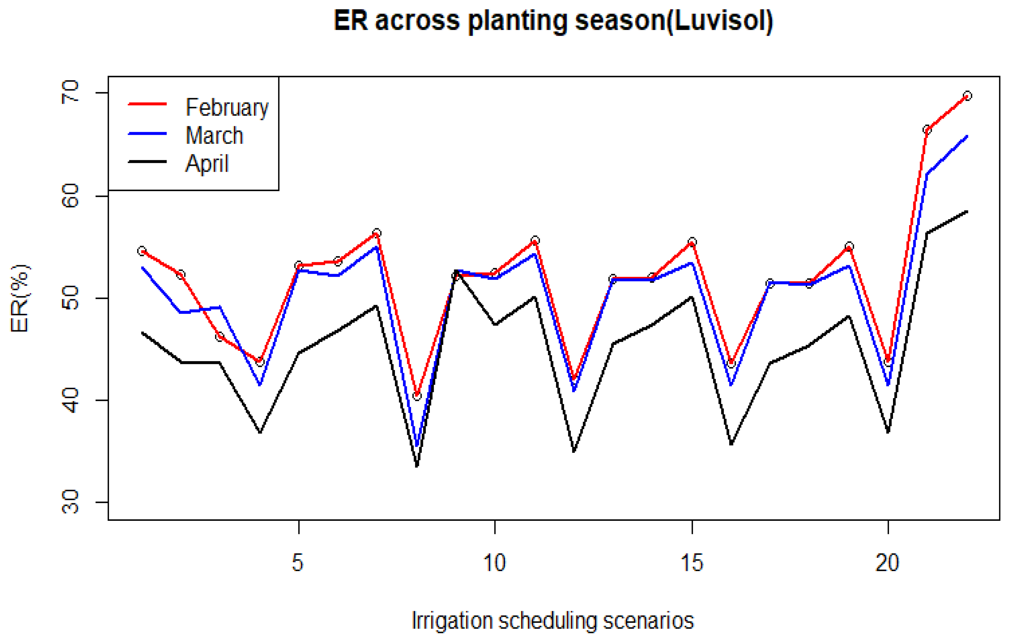
Figure A4.
Yield reduction over planting seasons (Luvisol).
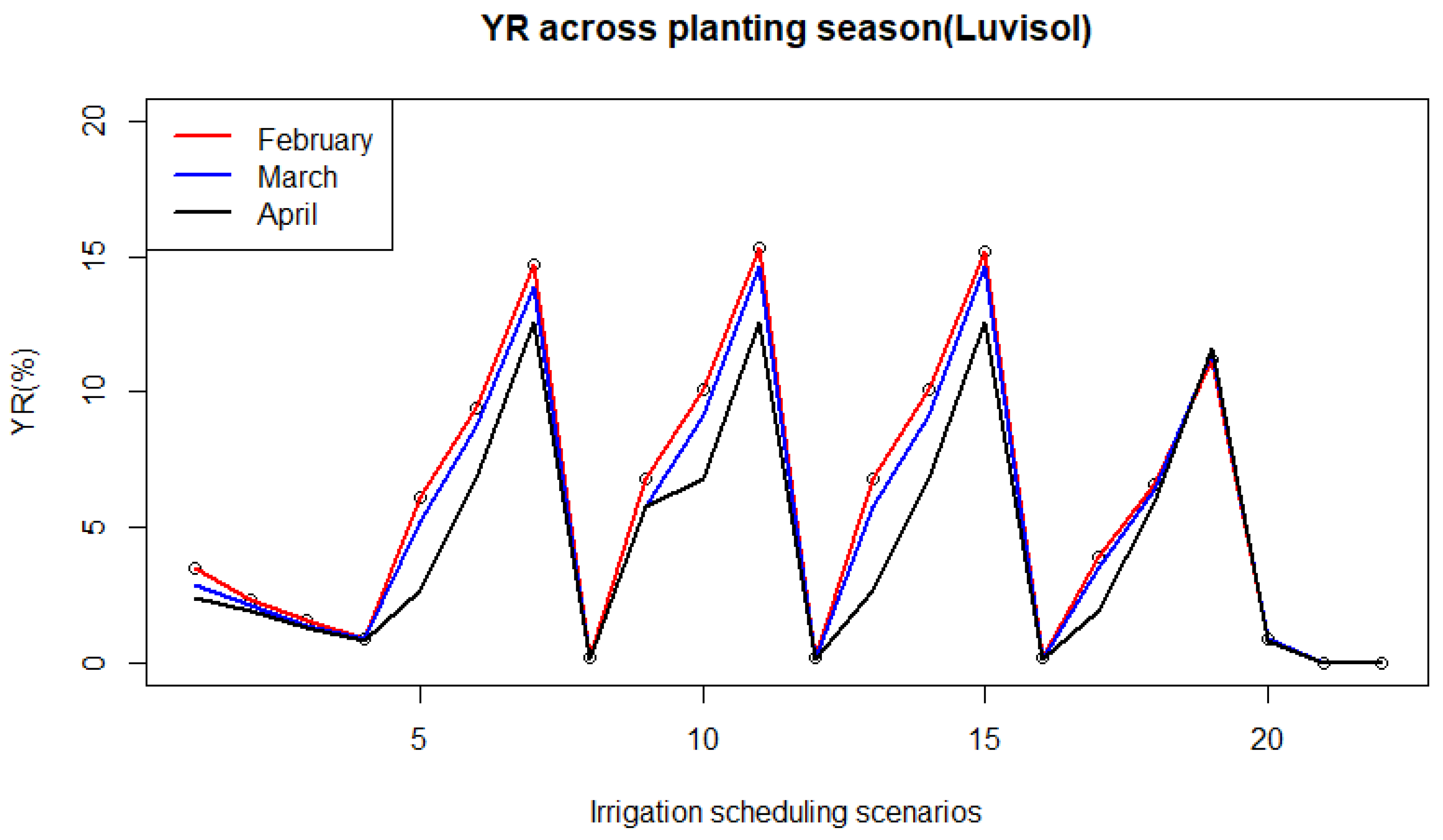
Figure A5.
Efficiency irrigation schedule over planting seasons (Vertisol).
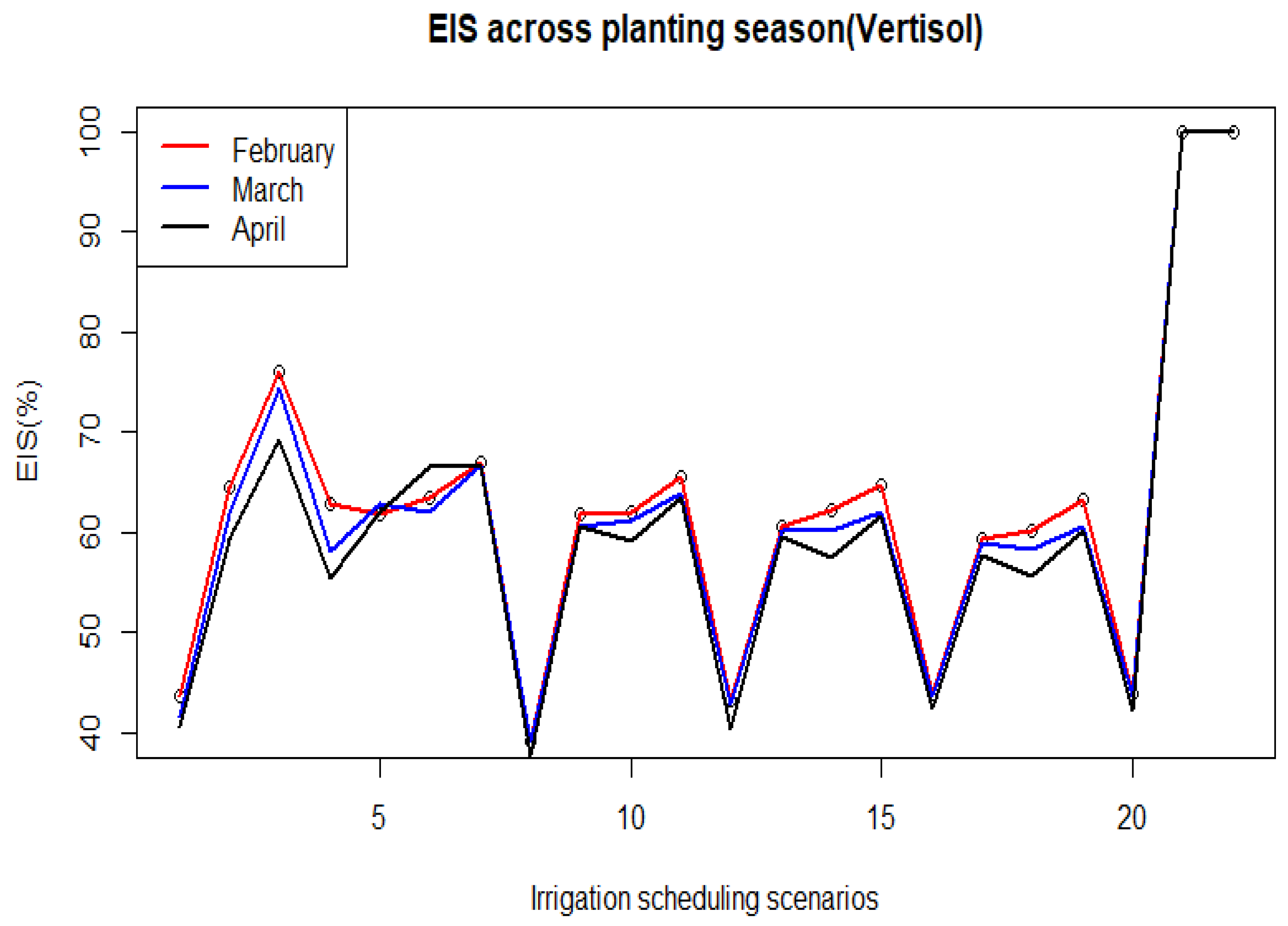
Figure A6.
Deficiency irrigation schedule over planting seasons (Vertisol).
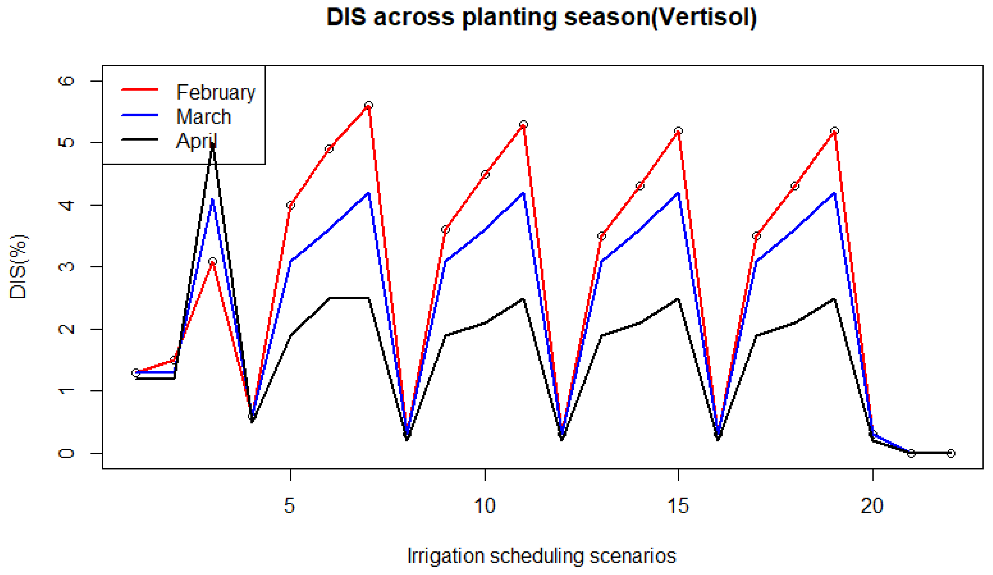
Figure A7.
Efficiency of rain over planting seasons (Vertisol).
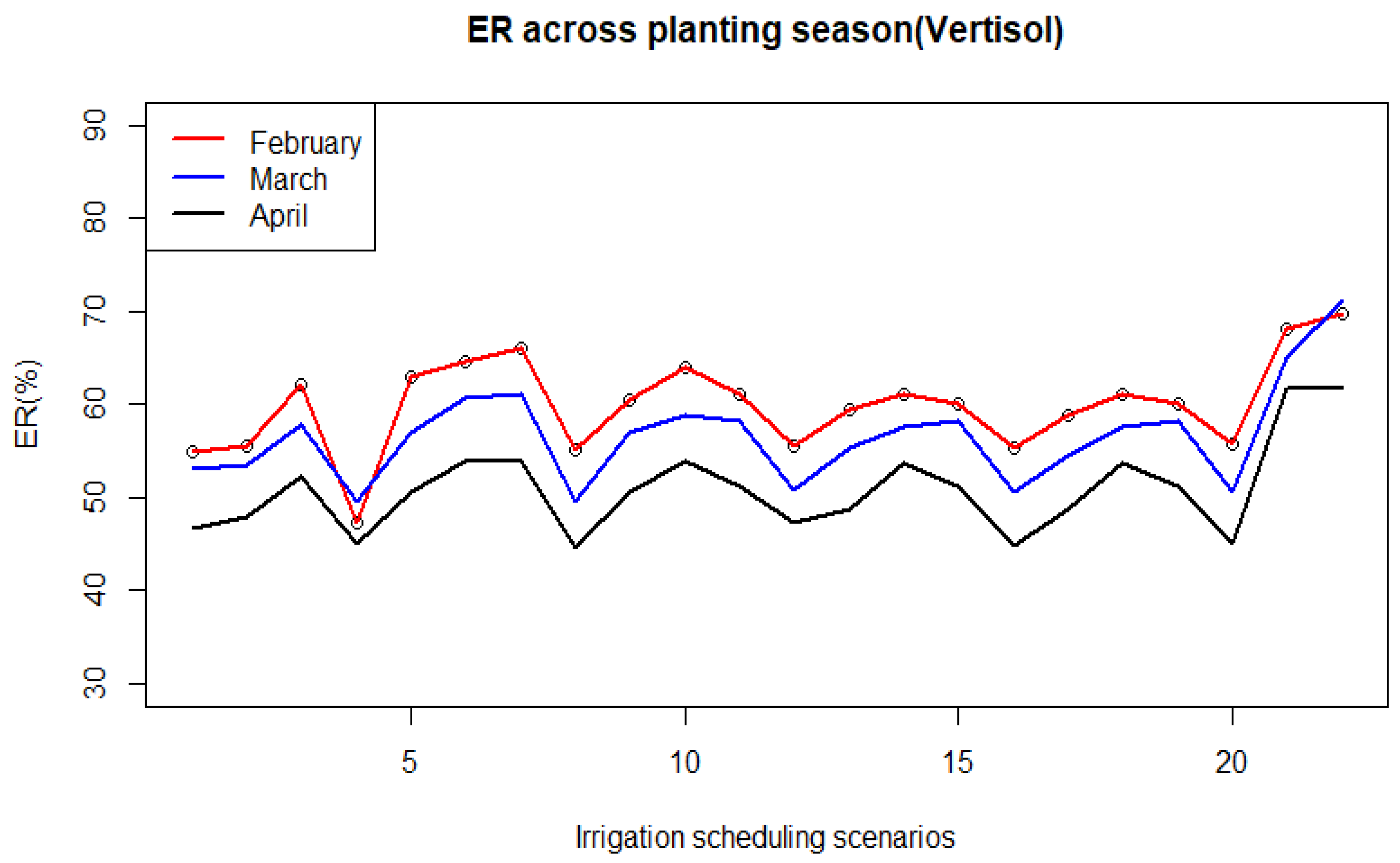
Figure A8.
Yield reduction over planting seasons (Vertisol).
References
- Abdelhafid, H., Gharb, I. and Maarouf, A. (2022) ‘Irrigation water demand management to address water scarcity’, Emirates Journal of Food and Agriculture [Preprint]. [CrossRef]
- Allen, R.G. et al. (1989) ‘FAO Irrigation and Drainage Paper’. FAO - Food and Agriculture Organization of the United Nations. Available at: https://www.fao.org/4/x0490e/x0490e00.htm.
- Awlachew, S.B. (2010) Irrigation Potential in Ethiopia. Colombo, Sri Lanka: International Water Management Institute, p. 60.
- Awulachew, S.B. et al. (2007) Water resources and irrigation development in Ethiopia. Colombo, Sri Lanka: International Water Management Institute.
- Balasaheb, K.S. and Biswal, S. (2020) ‘Study of Crop Evapotranspiration and Irrigation Scheduling of Different Crops Using Cropwat Model in Waghodia Region, India’, International Journal of Current Microbiology and Applied Sciences, 9(5), pp. 3208–3220. [CrossRef]
- Bekele, R.D. et al. (2024) ‘Irrigation technologies and management and their environmental consequences: Empirical evidence from Ethiopia’, Agricultural Water Management, 302, p. 109003. [CrossRef]
- Booker Tate (1998) ‘Operation and Maintenance manual for Fincha sugar esate’. Booker Tate.
- Booker Tate (2007) ‘Feasibility study and detailed design: Fincha Sugar esate’.
- Clemmens, A.J. and Molden, D.J. (2007) ‘Water uses and productivity of irrigation systems’, Irrigation Science, 25(3), pp. 247–261. [CrossRef]
- Etissa, E. et al. (2014) ‘Irrigation Water Management Practices in Smallholder Vegetable Crops Production: The Case of the Central Rift Valley of Ethiopia’, Science, Technology and Arts Research Journal, 3(1), pp. 74–83. [CrossRef]
- FAO (2015) ‘Water at a Glance: The relationship between water, agriculture, food security and poverty’.
- Gabr, M.E. and Fattouh, E.M. (2021) ‘Assessment of irrigation management practices using FAO-CROPWAT 8, case studies: Tina Plain and East South El-Kantara, Sinai, Egypt’, Ain Shams Engineering Journal, 12(2), pp. 1623–1636. [CrossRef]
- Geleta, C.D. (2019) ‘Effect of first watering month on water requirement of sugarcane using CROPWAT Model in Finchaa Valley, Ethiopia’, International Journal of Water Resources and Environmental Engineering, 11(1), pp. 14–23. [CrossRef]
- Grafton, R.Q., Williams, J. and Jiang, Q. (2017) ‘Possible pathways and tensions in the food and water nexus’, Earth’s Future, 5(5), pp. 449–462. [CrossRef]
- Habib (2002) Evalaution of Irrigation water application practices in Fincha sugar esate.
- Haile, G.G. et al. (2024) ‘Projected impacts of climate change on global irrigation water withdrawals’, Agricultural Water Management, 305, p. 109144. [CrossRef]
- Karuku, G. et al. (2014) ‘Use of CROPWAT model to predict water use in irrigated tomato production at Kabete, Kenya’.
- Khan, M.E. (2021) ‘SUGARCANE CROP DEVELOPMENTAL STAGES AND WATER REQUIREMENT: A REVIEW’.
- Kumari, S. (2017) ‘IRRIGATION SCHEDULING USING CROPWAT’.
- Moseki, O., Murray-Hudson, M. and Kashe, K. (2019) ‘Crop water and irrigation requirements of Jatropha curcas L. in semi-arid conditions of Botswana: applying the CROPWAT model’, Agricultural Water Management, 225, p. 105754. [CrossRef]
- Reta, B.G., Hatiye, S.D. and Finsa, M.M. (2024) ‘Crop water requirement and irrigation scheduling under climate change scenario, and optimal cropland allocation in lower kulfo catchment’, Heliyon, 10(10), p. e31332. [CrossRef]
- Soomro, S. et al. (2023) ‘Estimation of irrigation water requirement and irrigation scheduling for major crops using the CROPWAT model and climatic data’, Water Practice and Technology, 18(3), pp. 685–700. [CrossRef]
- Surendran, U. et al. (2015) ‘Modelling the Crop Water Requirement Using FAO-CROPWAT and Assessment of Water Resources for Sustainable Water Resource Management: A Case Study in Palakkad District of Humid Tropical Kerala, India’, Aquatic Procedia, 4, pp. 1211–1219. [CrossRef]
- Wabela, K. et al. (2022) ‘Optimization of Irrigation Scheduling for Improved Irrigation Water Management in Bilate Watershed, Rift Valley, Ethiopia’, Water, 14(23), p. 3960. [CrossRef]
- Zhou, T. et al. (2020) ‘Global Irrigation Characteristics and Effects Simulated by Fully Coupled Land Surface, River, and Water Management Models in E3SM’, Journal of Advances in Modeling Earth Systems, 12(10), p. e2020MS002069. [CrossRef]
Figure 2.
Multiple scatterplots for performance indicators (Luvisol ).
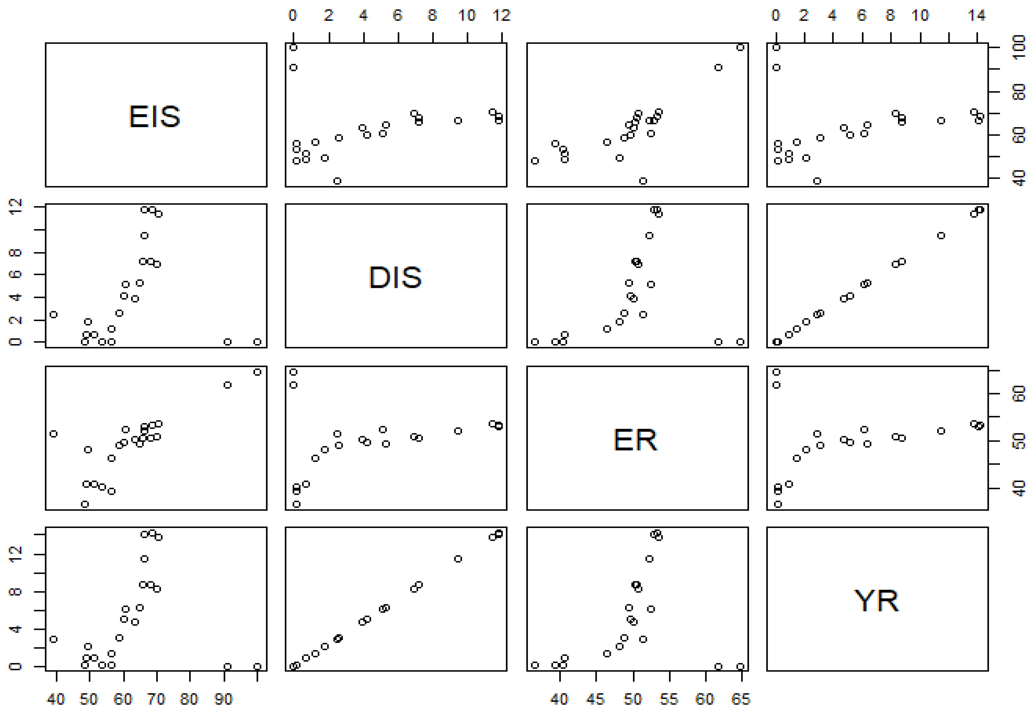
Figure 3.
Multiple scatterplots for performance indicators (Vertisol).
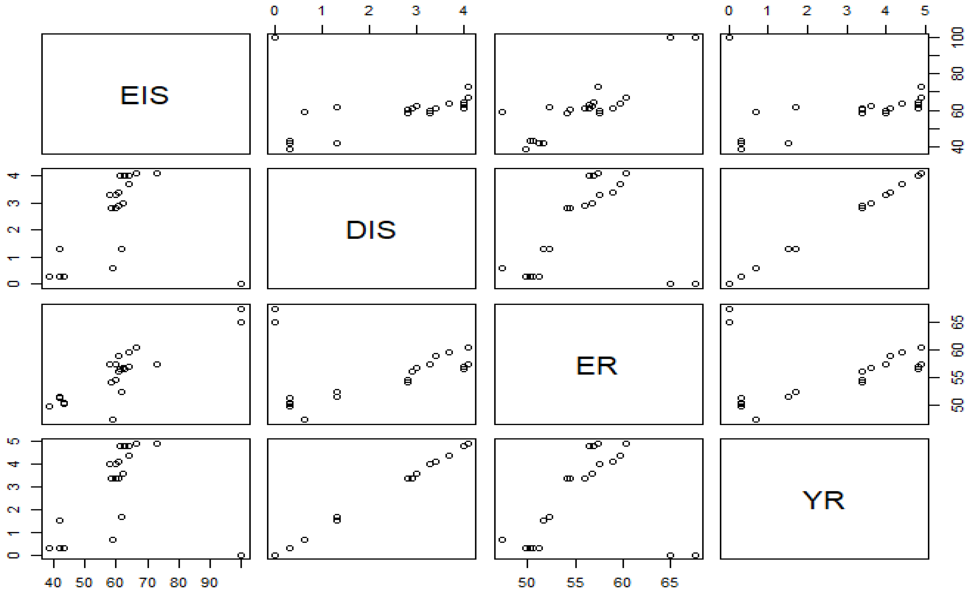
Table 1.
Soil data (Luvisols).
| Parameter | Values | Source |
| Total available soil moisture (FC - WP), mm/m | 130 | Field survey (Booker Tate, 2007) |
| Maximum rain infiltration rate, mm/day | 40 | FAO(Allen et al., 1989). |
| Maximum rooting depth, cm | 90 | Field survey (Booker Tate 2007) |
| Initial soil moisture depletion (as % TAM) | 50 | Consideration |
Table 2.
Soil data (Vertisols).
| Parameter | Values | Source |
| Total available soil moisture (FC - WP) mm/m | 250 | Field survey (Booker Tate, 2007) |
| Maximum rain infiltration rate, mm/day | 30 | FAO |
| Maximum rooting depth, cm | 90 | Field survey (Booker Tate, 2007) |
| Initial soil moisture depletion (as % TAM) | 50 | Consideration |
Table 3.
Long year average climate (CROPWAT 8.0).
| Month | Min Temp, CO | Max Temp | Humidity | Wind | Sun | Rad | ETo | Rainfall |
| °C | °C | % | km/day | hours | MJ/m²/day | mm/day | mm | |
| January | 12.5 | 32.2 | 22 | 57 | 9 | 20.6 | 3.81 | 2.7 |
| February | 14.4 | 33.6 | 24 | 61 | 9 | 21.9 | 4.3 | 4.3 |
| March | 16.5 | 34.1 | 25 | 60 | 9.1 | 23.3 | 4.7 | 27 |
| April | 17.6 | 33.9 | 26 | 58 | 8.4 | 22.5 | 4.72 | 42.4 |
| May | 16.9 | 32.3 | 25 | 55 | 8.6 | 22.3 | 4.56 | 133.3 |
| June | 16.3 | 29.8 | 23 | 53 | 7.1 | 19.7 | 4.07 | 208.6 |
| July | 15.9 | 27.2 | 22 | 44 | 5 | 16.7 | 3.48 | 318.8 |
| August | 15.6 | 26.5 | 21 | 43 | 5.1 | 17.1 | 3.45 | 273.7 |
| September | 15.1 | 28 | 22 | 45 | 7.3 | 20.4 | 3.84 | 192.2 |
| October | 14 | 29.6 | 22 | 46 | 9.1 | 22.3 | 3.97 | 79.2 |
| November | 13 | 30.5 | 22 | 51 | 9.4 | 21.4 | 3.78 | 16.4 |
| December | 12.2 | 31.3 | 22 | 57 | 8.7 | 19.7 | 3.62 | 4.2 |
| Average | 15 | 30.8 | 23 | 52 | 8 | 20.6 | 4.02 |
Table 4.
Crop data of sugarcane –virgin.
| Growth stages | |||||
| Characteristics | Initial stage | Crop development | Mid-season | Late & harvest | Source |
| Rooting depth | 0.30m | 0.60 | 0.90 | - | Field survey (Booker Tate, 2007) |
| Length of period | 50 days | 70 days | 220 days | 140 days | FAO |
| Kc | |||||
| 0.4 | >> | 1.25 | 0.75 | FAO | |
| 0.45 | >> | 1.2524 | 0.7524 | FAO Adjusted | |
| Critical water content | 0.65 | 0.65 | 0.65 | 0.65 | FAO |
| Yield response factor (ky) | 0.75 | - 0.75 | 0.5 | 0.1 | FAO |
| 0.5 | 0.75 | 1.2 | 0.1 | CROPWAT file | |
| 0.75 | 0.75 | 1.2 | 0.1 | FAO Adjusted | |
| Max Crop Height | 3m | ||||
Table 11.
Analysis of variance (ANOVA) table for efficiency irrigation scheduling (Luvisols).
| source of variation | Degree of freedom | sum of squares | Mean square | computed F | Pr (>F) |
| Factor (Irrigation scheduling scenarios) | 21 | 11543 | 549.7 | 146.05 | < 2e-16 *** |
| Replication | 2 | 99 | 49.3 | 13.09 | 3.81e-05 *** |
| Error | 42 | 158 | 3.8 |
CV= 3.1%, ns – no significance test and Signif Codes- 0 ‘***’ 0.001 ‘**’ 0.01 ‘*’.
Table 12.
Analysis of variance (ANOVA) table for Deficiency irrigation schedule ( Luvisols).
| source of variation | Degree of freedom | sum of squares | Mean square | computed F | Pr (>F) |
| Factor (Irrigation scheduling scenarios) | 21 | 1064.1 | 50.67 | 131.7 | < 2e-16 *** |
| Replication | 2 | 14 | 7 | 18.2 | 2.03e-06 *** |
| Error | 42 | 16.2 | 0.38 |
CV=14.5%, ns – no significance test and Signif Codes- 0 ‘***’ 0.001 ‘**’ 0.01 ‘*’.
Table 13.
Analysis of variance (ANOVA) table for Efficiency rain ( Luvisols).
| source of variation | Degree of freedom | sum of squares | Mean square | computed F | Pr (>F) |
| Factor (Irrigation scheduling scenarios) | 21 | 2909 | 138.52 | 67.81 | <2e-16 *** |
| Replication | 2 | 530.2 | 265.09 | 129.76 | <2e-16 *** |
| Error | 42 | 85.8 | 2.04 |
CV= 2.9 %, ns – no significance test and Signif Codes- 0 ‘***’ 0.001 ‘**’ 0.01 ‘*’.
Table 14.
Analysis of variance (ANOVA) table for yield reduction ( Luvisols).
| source of variation | Degree of freedom | sum of squares | Mean square | computed F | Pr (>F) |
| Factor (Irrigation scheduling scenarios) | 21 | 1529.4 | 72.83 | 131.06 | < 2e-16 *** |
| Replication | 2 | 21 | 10.49 | 18.88 | 1.42e-06 *** |
| Error | 42 | 23.3 | 0.56 |
CV=14.5 %, ns – no significance test and Signif Codes- 0 ‘***’ 0.001 ‘**’ 0.01 ‘*’.
Table 15.
Analysis of variance (ANOVA) table for efficiency irrigation scheduling (Vertisol).
| source of variation | Degree of freedom | sum of squares | Mean square | computed F | Pr (>F) |
| Factor (Irrigation scheduling scenarios) | 21 | 15342 | 730.6 | 414.76 | < 2e-16 *** |
| Replication | 2 | 60 | 29.8 | 16.91 | 4.1e-06 *** |
| Error | 42 | 74 | 1.8 |
CV= 2.2%, ns – no significance test and Signif Codes- 0 ‘***’ 0.001 ‘**’ 0.01 ‘*’.
Table 16.
Analysis of variance (ANOVA) table for Deficiency irrigation schedule ( Luvisols).
| source of variation | Degree of freedom | sum of squares | Mean square | computed F | Pr (>F) |
| Factor (Irrigation scheduling scenarios) | 21 | 160.44 | 7.64 | 16.75 | 3.57e-14 *** |
| Replication | 2 | 16.39 | 8.193 | 17.96 | 2.31e-06 *** |
| Error | 42 | 19.16 | 0.456 |
CV=29.9%, ns – no significance test and Signif Codes- 0 ‘***’ 0.001 ‘**’ 0.01 ‘*’.
Table 17.
Analysis of variance (ANOVA) table for Efficiency rain (Vertisol).
| source of variation | Degree of freedom | sum of squares | Mean square | computed F | Pr (>F) |
| Factor (Irrigation scheduling scenarios) | 21 | 1517.5 | 72.3 | 38.91 | <2e-16 *** |
| Replication | 2 | 932.9 | 466.4 | 251.13 | <2e-16 *** |
| Error | 42 | 78 | 1.9 |
CV= 2.4 %, ns – no significance test and Signif Codes- 0 ‘***’ 0.001 ‘**’ 0.01 ‘*’.
Table 18.
Analysis of variance (ANOVA) table for yield reduction (Vertisol).
| source of variation | Degree of freedom | sum of squares | Mean square | computed F | Pr (>F) |
| Factor (Irrigation scheduling scenarios) | 21 | 230.35 | 10.969 | 16.64 | 3.98e-14 *** |
| Replication | 2 | 24.71 | 12.357 | 18.75 | 1.52e-06 *** |
| Error | 42 | 27.68 | 0.659 |
CV=29.9 %, ns – no significance test and Signif Codes- 0 ‘***’ 0.001 ‘**’ 0.01 ‘*’.
Table 19.
Mean separation for scheduling performance indicators (Luvisols).
| EIS | DIS ( Increasing order) |
ER | YR ( Increasing order) |
||||
| Scenarios | Groups | Scenarios | Groups | Scenarios | Groups | Scenarios | Groups |
| 22 | a | 22 | h | 22 | a | 22 | h |
| 21 | b | 21 | h | 21 | a | 21 | h |
| 7 | c | 12 | h | 7 | b | 12 | h |
| 6 | cd | 16 | h | 11 | b | 16 | h |
| 11 | cd | 8 | h | 15 | b | 8 | h |
| 10 | cd | 20 | gh | 9 | bc | 20 | gh |
| 15 | cde | 4 | gh | 19 | bc | 4 | gh |
| 19 | cdef | 3 | gh | 1 | bc | 3 | gh |
| 14 | cdef | 2 | gh | 6 | bcd | 2 | gh |
| 18 | cdefg | 1 | fg | 10 | bcd | 1 | fg |
| 5 | defg | 17 | fg | 14 | bcd | 17 | fg |
| 9 | efgh | 5 | ef | 5 | bcd | 5 | ef |
| 13 | fghi | 13 | ef | 13 | bcd | 13 | ef |
| 17 | ghi | 9 | de | 18 | bcd | 9 | de |
| 3 | hij | 18 | cde | 17 | bcd | 18 | cde |
| 12 | hij | 6 | cd | 2 | cd | 6 | cd |
| 16 | ijk | 10 | c | 3 | d | 10 | c |
| 20 | jk | 14 | c | 20 | e | 14 | c |
| 2 | k | 19 | b | 4 | e | 19 | b |
| 4 | k | 7 | ab | 16 | e | 7 | ab |
| 8 | k | 15 | a | 12 | e | 15 | a |
| 1 | l | 11 | a | 8 | e | 11 | a |
Note: Treatments with the same letter are not significantly different.
Table 20.
Mean separation for scheduling performance indicators (Vertisols ).
| EIS | DIS ( Increasing order) |
ER | YR ( Increasing order) |
||||
| Scenarios | Groups | Scenarios | Groups | Scenarios | Groups | Scenarios | Groups |
| 22 | a | 22 | c | 22 | a | 22 | c |
| 21 | a | 21 | c | 21 | a | 21 | c |
| 3 | b | 12 | c | 7 | b | 12 | c |
| 7 | c | 16 | c | 6 | b | 16 | c |
| 11 | cd | 20 | c | 10 | bc | 20 | c |
| 6 | cd | 8 | c | 14 | bcd | 8 | c |
| 15 | cde | 4 | c | 18 | bcd | 4 | c |
| 5 | def | 1 | bc | 3 | bcd | 1 | bc |
| 2 | def | 2 | bc | 11 | bcd | 2 | bc |
| 19 | def | 13 | ab | 5 | bcd | 13 | ab |
| 9 | def | 17 | ab | 15 | bcde | 17 | ab |
| 10 | def | 9 | ab | 19 | bcde | 9 | ab |
| 13 | def | 5 | ab | 9 | bcdef | 5 | ab |
| 14 | def | 14 | ab | 13 | cdefg | 14 | ab |
| 4 | ef | 18 | ab | 17 | defgh | 18 | ab |
| 17 | ef | 10 | ab | 2 | efgh | 10 | ab |
| 18 | f | 6 | a | 1 | fghi | 6 | a |
| 16 | g | 15 | a | 12 | ghi | 15 | a |
| 20 | g | 19 | a | 20 | ghi | 19 | a |
| 12 | gh | 11 | a | 16 | ghi | 11 | a |
| 1 | gh | 3 | a | 8 | hi | 3 | a |
| 8 | h | 7 | a | 4 | i | 7 | a |
Note: Treatments with the same letter are not significantly different.
Disclaimer/Publisher’s Note: The statements, opinions and data contained in all publications are solely those of the individual author(s) and contributor(s) and not of MDPI and/or the editor(s). MDPI and/or the editor(s) disclaim responsibility for any injury to people or property resulting from any ideas, methods, instructions or products referred to in the content. |
© 2025 by the authors. Licensee MDPI, Basel, Switzerland. This article is an open access article distributed under the terms and conditions of the Creative Commons Attribution (CC BY) license (http://creativecommons.org/licenses/by/4.0/).
Copyright: This open access article is published under a Creative Commons CC BY 4.0 license, which permit the free download, distribution, and reuse, provided that the author and preprint are cited in any reuse.


