Submitted:
26 August 2025
Posted:
23 September 2025
You are already at the latest version
Abstract
Competition Lotka-Volterra models is studied, which is an extension of linear diffusion model in $\cite{25}$. In this paper, we study pattern formation solutions for this ecological system with a nonlinear diffusion part which represents both self-diffusion and cross-diffusion. The role of crucial cross diffusion $\beta_2$ in developing Patterns has been shown. Turing instability conditions have been derived and illustrated numerically. Furthermore, the Turing bifurcation Threshold region is verified. Labyrinthine patterns under cross-diffusion $\beta_2 < 0$ which may used for modeling the interactions in crystals has been found. Furthermore, spot patterns via self-diffusion $\alpha_1 < 0 $ have been shown. Numerical solutions through finite element method is applied to show those types of pattern formations for our model.
Keywords:
Turing instability
; cross-diffusion
; finite-element modeling
; crystal growth patterns
1. Introduction
In the subsequent decades, researchers developed and refined various reaction-diffusion models, exploring their applications in different fields, especially in Ecology ([2,6,18]). The Lotka- voltera model is defined by Lotka (1925) in [27] and Volterra (1926) in [28] describes the interaction of two species in competition models for the same resources and is mathematically explained with a negative sign. The Lotka-Volterra competition model with linear diffusion term has been studied widely ([12,13,20,25,31,32,33,34]). Besides that, the dynamics of predator-prey interactions were also interactive for studying some complex phenomena. The integration of nonlinear diffusion into these models added a new layer of complexity and realism to pattern formation studies. The foundation for reaction-diffusion models can be traced back to the work of Alan Turing in 1952 ([4]). Turing’s seminal paper, “The Chemical Basis of Morphogenesis,” demonstrated how reaction-diffusion systems could generate complex patterns. This work laid the groundwork for the study of pattern formation in nonlinear systems. In [30], with a typical Lotka–Volterra–Gause reaction-diffusion model and constant diffusion coefficient the producing of a pattern was not achieved, however, the existence of non-linear diffusion in Shigesada-Kawasaki-Teramoto (SKT) model was enough to build patterns and establish Turing instability. In the context of ecology, non-linear diffusion manifests as either cross-diffusion or self-diffusion. Cross-diffusion refers to the phenomenon where the movement of one species affects the diffusion of another species, whereas self-diffusion describes the spread of individuals within the same species. Both theoretical models and experimental studies have demonstrated that cross-diffusion significantly contributes to the formation of spatial patterns [1,3,11]. Specifically, cross-diffusion mechanisms are crucial in explaining how species interactions can lead to complex pattern formation, such as stripes, spots, or labyrinthine structures in population distributions. This model extends the focus on pattern formations as in SKT model ecology system as in [25] and to bridges the ecology with solid state system by adapting nonlinear diffusion effect in crystal growth. One of the pivotal concepts in understanding pattern formation through diffusion processes is Turing instability. This instability arises when the diffusion rates of interacting species lead to the spontaneous emergence of spatial patterns. To theoretically verify the presence of Turing instability in a given ecological model, four specific conditions must be satisfied. These conditions, detailed in the works of Barrio et al. (1999), Othmer et al. (2009), and Page et al. (2005) provide a rigorous framework for predicting and analyzing pattern formation due to non-linear diffusion [8,9,10]. The system we will study is
where
and are the interaction species as a function of x and t. The diffusion coefficients are nonlinear, while the reaction term includes logistic growth of second order and , the cooperation within species are defined by the terms and , while the competition terms are and . All parameters are positive. Note that this model is studied before in [25] in the case of constant diffusion coefficients. Pattern formation is absent for constant diffusion in [25] and the reaction terms with different parameter values was not sufficient to produce any type of pattern solutions. Therefore, we extend the study to nonlinear diffusion coefficients and we include various forms of non-linear diffusion.
The initial conditions are
and boundary conditions
where L is the length of domain x.
2. Steady State Solutions
Steady-state solutions are the intersection points of the two reaction parts in (1)
where and .
Our work focuses on studying the existence of a pattern for (1) at the positive coexistence steady state solutions of (5). The existence and stability of are studied in detail in [25] and have been categorized into seven topological regions. The maximum number of coexistence steady states are three. Furthermore, two types of bifurcation have been also shown for this model in [25]. Namely, Saddle-Node and Transcritical bifurcation.
3. Conditions of Turing Instability
In this section, we will examine the probability of the emergence of patterns for 1. We will follow the hypothesis, that the change of stability of the steady state solution under the impact of diffusion term may lead to the existence of patterns. The linear stability analysis will be used in the following sections to find the critical wave number and critical value for the bifurcation parameter. The Turing conditions will be derived for the cases, without and with diffusion terms. This can be done using linearisation concepts.
4. Linearization of Reaction System
Firstly, we study the stability of in (5) and we exclude the diffusion term. We follow the same technique as in (Cross & Greenside, 2009; Turing, 1990) [14,16]. We introduce small perturbations around the steady state so that and , where . Now we replace and in (5) with and differentiate the left side, then we get
The characteristic equation of 6 arises from
where and are refers to the trace and the determinant of K, respectively and mathematically are defined to be
where
The steady state is stable if
In the rest of the paper, we focus on steady-state solutions which satisfy the two conditions in (10), i.e. we study stable in the case of missing diffusion part. Next, we try to find if it is possible to break at least one of the conditions in (10) by adding the diffusion term. This will help us to investigate the region where may pattern solution exists in (1).
5. Linearization of Reaction-Diffusion System (RDS)
The linearization in this section will cover three cases depending on the form we give to in the diffusion term. The linearization of (1) and (2) is
where
and K is the same as in 4. We assume solutions of the form where , then the dispersion relation can be obtained in the form
where
Turing instability states that the values of in (11) should be at least one positive. This will break the stability of and support the hypothesis of the existence of patterns. This can be done whenever either or , where:
In the following, we will focus on satisfying the first Turing condition . Next, we try to define regions of the Turing instability and Turing bifurcation Threshold depending on the parameters in (2). For this purpose we fixed the parameters in reaction term 5, i.e. we put , , and to get the numerical steady state . A simple calculation using MATLAB program shows that the positive steady state satisfies the conditions in 10 and therefore is stable. In Figure 1a–c, three regions of Pattern formation are defined for the parameter values of as the x-axis and as the y-axis. In the black regions, Turing instability conditions are satisfied, and unstable eigenvalues can be found.
5.1. Turing Bifurcation Threshold
The Turing bifurcation Threshold is the minimum values of the wave number which make for the parameter values in the nonlinear diffusion term (2). Figure 2 explains the region of Threshold, where represented by and by and, when , . The unstable region is above the Threshold curve while the stable region is under the threshold curve. Furthermore, we show positive eigenvalues of (11) whenever . This leads to change of the stability of steady state solutions with the present of diffusion term as can be seen in Figure 3, the values are and , , , , and . The steady-state loses stability and becomes unstable for some values of wave number . Thus, we conclude that the stability of can be broken under the effect of the non-linear diffusion term. Next, we show the type of pattern solutions for our model and general nonlinear diffusion, cross-diffusion, and self-diffusion forms.
6. Pattern Formations for RDS (1) and (2) in Two Dimensions
In this section, we have used one of the efficient numerical methods, the Finite element method to find high-quality forms of patterns in the defined regions. The Turing instability conditions have been applied in the previous sections to our model in (1) and (2) and support the idea of existing patterns in our model. The Finite element software package namely COMSOL Multiphysics will applied next to study some type of patterns depending on the initial conditions and the domain size. The domain we choose is square with and , where . The mesh size is of type extra fine resolution. The method of time stepping Backward differentiation formula(BDF) with adoptive mesh is used, and the convergence criteria; relative tolerance of order is applied to all the variables. The boundary conditions are of type zero-flux boundary conditions, while the initial conditions are chosen to be near the steady state solution and with small perturbation
The boundary conditions are expressed as , , , . Simulations use COMSOL Multiphysics with time to ensure pattern convergence. For the consistency with theoretical results in the previous section, we choose the same parameters and the numerical steady-state value of . However, we vary the parameters in (2) to show the patterns for the case of general nonlinear diffusion and both cross-diffusion and self-diffusion. In Figure 4a,b, we assume the case of self-diffusion by setting the parameters as follows: , and . The pattern solutions for both and show different forms of nice decoration of patterns. In Figure 4c,d, the nonlinearity of diffusion is defined to be cross-diffusion by setting , and .
The similarity in the patterns can be seen for both and . Another form of patterns have been produced as shown in Figure 5a–d. This time we choose to be negative in Figure 5a,b and positive in Figure 5c,d.
In the solid state, the diffusion rates of different species generally differ by several orders of magnitude. This is because they are typically governed by nonlinear Arrhenius escape rates, , where the migration barrier E can range from fractions of an electron volt to several electron volts. In other words, the diffusion term in the solid state model can be written as a nonlinear term (similar to the case in our model)during the diffusion of different materials in the solid form till it ends up producing some shape of patterns. For example, the competition between Crystal materials that produce some types of Patterns forms [35,36]. Figure 5 and Figure 6 illustrate the pattern formation that emerges from unstable fixed points, or stationary states, which have been spatially perturbed using Gaussian functions. The numerical simulations display regions characterized by periodic structures, which are interspersed with irregular and complex boundaries. This pattern bears a resemblance to grain boundaries observed in multi-crystal materials. The intriguing complexity of these patterns stems from the unique characteristics of the specific model under study.
7. Conclusions
In this paper, we extend the study of a Reaction-Diffusion model in Ecology, with two interaction species. The reaction terms represent competition between two species and cooperation within species. The spatial uniform solutions for this reaction equation have been previously studied but only with constant diffusion terms. However, we expand the study of this model assuming that the diffusion coefficient is nonlinear. We have shown that this model satisfied the Conditions of Turing instability for specific steady-state solutions and for some values of wave number theoretically. Then we studied the pattern formation solutions for this model with nonlinear Diffusion coefficients using COMSOL MULTIPHYSICS software. We demonstrate diverse Patterns for different values of parameters in the Diffusion coefficient terms specially when we have the cases of cross- and self-diffusion. The regions where patterns can be formulated depending on two parameters in Diffusion coefficient parts have been classified. Finally, the Turing bifurcation Threshold has been found and plotted for a numerical steady-state solution. Unlike the constant diffusion model ([25]), our extended model has exhibits Turing instability and produce some types of Pattern solutions.
Author Contributions
This work was written with equal contributions from each author.
Funding
Not applicable.
Institutional Review Board Statement
The authors state that this research paper complies with ethical standards. This research paper does not involve either human participants or animals.
Data Availability Statement
Data sharing does not apply to this article as no data sets were generated or analyzed during the current study.
Conflicts of Interest
The authors declare that they have neither financial nor conflict of interest.
References
- Y. Almirantis, S. Papageorgiou, Cross–diffusion effects on chemical and biological pattern formation, J. Theor. Biol. 151 (1991) 289–311. [CrossRef]
- Murray JD. Parameter space for Turing instability in reaction-diffusion mechanisms: a comparison of models. J Theor Biol 1982;98:143–63. [CrossRef]
- V.K. Vanag, I.R. Epstein, Cross–diffusion and pattern formation in reaction-diffusion system, Phys. Chem. Phys. 11 (2009) 897–912. [CrossRef]
- Turing AM. The Chemical Basis of Morphogenesis: Philosophical Transactions of the Royal Society of London. Ser. B, Biol. Sci., vol. 237, 1952. [CrossRef]
- Y. Peng, T. Zhang, Stability and Hopf bifurcation analysis of a gene expression model with diffusion and time delay, Abstr. Appl. Anal. 2014 (2014) 1. [CrossRef]
- A. Okubo, Diffusion and Ecological Problems: Mathematical Models, Biomathematics, Springer–Verlag, Berlin, Heidelberg, 1980. [CrossRef]
- L.A. Segel, J.L. Jackson, Dissipative structure: an explanation and an ecological example, J. Theor. Biol. 37 (1972) 545–559. [CrossRef]
- Maxime Breden, Christian Kuehn, Cinzia Soresina. On the influence of cross-diffusion in pattern formation. Journal of Computational Dynamics, (2021), 8 (2), pp.213. [CrossRef]
- T. Zhang, Y. Xing, H. Zang, M. Han, Spatiotemporal dynamics of a reaction-diffusion system for a predator-prey model with hyperbolic mortality, Nonlinear Dyn. 78 (2014) 265–277. [CrossRef]
- Page KM, Maini PK, Monk NAM. Complex pattern formation in reaction-diffusion systems with spatially varying parameters. Phys D Nonlinear Phenom 2005;202:95–115. [CrossRef]
- Nanako Shigesada, Kohkichi Kawasaki, and Ei Teramoto. Spatial segregation of interacting species. Journal of Theoretical Biology, 79(1):83–99, 1979. [CrossRef]
- Dunbar SR. Traveling wave solutions of diffusive Lotka-Volterra equations: a heteroclinic connection in R4. Trans Am Math Soc 1984:557–94. [CrossRef]
- Woolley, T. E., Krause, A. L., & Gaffney, E. A. (2021). Bespoke Turing systems. Bulletin of Mathematical Biology, 83, 1-32. [CrossRef]
- Cross M, Greenside H. Pattern formation and dynamics in nonequilibrium systems. Cambridge University Press; 2009. [CrossRef]
- Rasheed SM. Pattern Formation for a New Model of Reaction-Diffusion System. 2018 Int. Conf. Adv. Sci. Eng., IEEE; 2018, p. 99–104.
- Turing AM. The chemical basis of morphogenesis. Bull Math Biol 1990;52:153–97. [CrossRef]
- Li, S., & Ling, L. (2020). Complex pattern formations by spatial varying parameters. Advances in Applied Mathematics and Mechanics, 12(6), 1327–1352. [CrossRef]
- F. Brauer. On the populations of Competing Species. Mathematical Biosciences, vol. 19, (1974), 299-306. [CrossRef]
- K. Gopalsamy. Exchange of Equilibria in Two Species Lotka-Voltera Competition Models. J. Austral. Math. Soc., vol. 24, (1982), 160–170. [CrossRef]
- J.F. AL-Omari, S. A. Gourley. Stability And Travelling Fronts In Lotka-Voltera Competition Models With Stage Structure. J. Appl. Math, vol. 63, (2003), 2063–2086. [CrossRef]
- S. A. Gourley. Two-Species Competition With High Dispersal: The Winning Strategy. Mathematical Biosciences And Engineering, vol.2, No.2 (2005), 345-362. [CrossRef]
- V. Volpert, S.Petrovskii. Reaction-diffusion waves in biology. Physics of Life Reviews, vol.6, (2009), 267-310. [CrossRef]
- Y. Hosono. Travelling Waves For A Diffusive Lotka-Volterra Competition Model I: Singular Perturbations. Discrete And Continous Dynamical Systems-Series B, vol. 3, (2003), 97-95. [CrossRef]
- Z. Li. Asymptotic Behaviour of Travelling Wavefronts of Lotka-Volterra Competitive System. Int. Journal of Math. Analysis, vol. 2, (2008), 1295–1300.
- Rasheed, Shaker M., and J. Billingham. A Reaction-Diffusion Model for Inter-Species Competition and Intra-Species Cooperation. Mathematical Modelling of Natural Phenomena 8.3 (2013): 154-181. [CrossRef]
- Krebs, C.J., 1994. Ecology—The Experimental Analysis of Distribution and Abundance, 4th ed. Harper Collins College Publishers, New York, p. 801.
- Lotka, A.J., 1925. Elements of Physiological Biology. Dover Publications, New York, 1956.
- Volterra, V., 1926. Fluctuation in the abundance of a species considered mathematically. Nature 118, 558–560. [CrossRef]
- Breden, M., Kuehn, C., Soresina, C. (2019). On the influence of cross-diffusion in pattern formation. arXiv preprint arXiv:1910.03436. [CrossRef]
- Kazuo Kishimoto and Hans F. Weinberger. The spatial homogeneity of stable equilibria of some reaction-diffusion systems on convex domains. Journal of Differential Equations, 58:15–21, 1985. [CrossRef]
- J.D. Murray. Mathematical Biology I: An introduction. Springer-Verlag, New York, 2002.
- K. Gopalsamy. Exchange of Equilibria in Two Species Lotka-Voltera Competition Models. J. Austral. Math. Soc., vol. 24, (1982), 160–170. [CrossRef]
- N. Britton. Reaction-Diffusion Equations And Their Applications To Biology. Academic Press INC. (London) LTD, 1986. [CrossRef]
- Y. Hosono. Travelling Waves For A Diffusive Lotka-Volterra Competition Model I: Singular Perturbations. Discrete And Continous Dynamical Systems-Series B, vol. 3, (2003), 97-95. [CrossRef]
- Turing Instability in the Solid State: Void Lattices in Irradiated Metals Phys. Rev. Lett. 124, (2020),167-401. [CrossRef]
- F.A. dos S. Silva, R.L. Viana, S.R. Lopes, Pattern formation and Turing instability in an activator-inhibitor system with power-law coupling, Physica A 419 (2015) 487–497. [CrossRef]
Figure 1.
The region of existing Pattern formation according to the value of the parameters as x-axis and as y-axis. The black regions are the regions where pattern formation solutions are supposed to exist and the condition of Turing instability should be satisfied.
Figure 1.
The region of existing Pattern formation according to the value of the parameters as x-axis and as y-axis. The black regions are the regions where pattern formation solutions are supposed to exist and the condition of Turing instability should be satisfied.
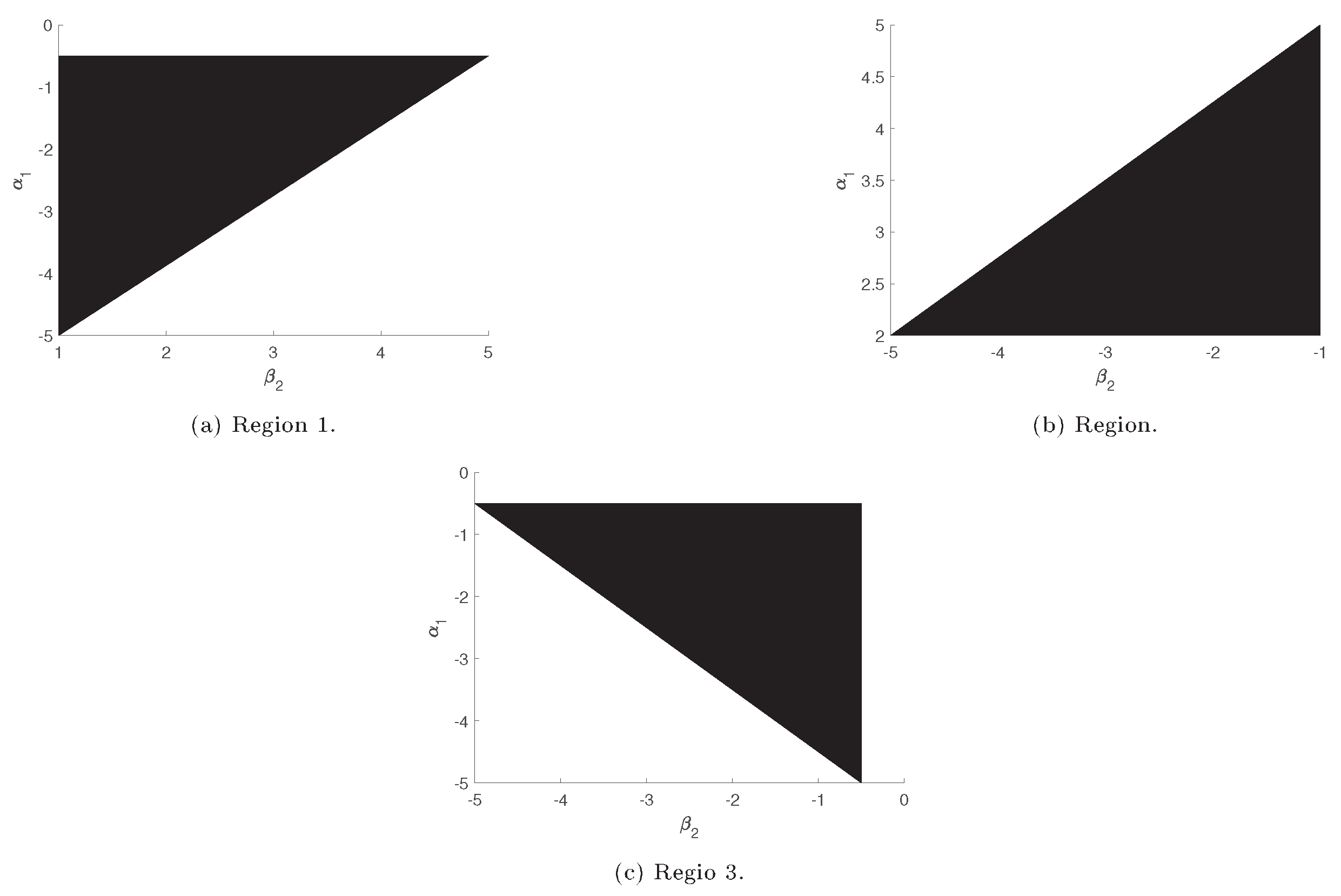
Figure 2.
Turing bifurcation threshold region . is and wave number represents . The parameters are, , , , , and .
Figure 2.
Turing bifurcation threshold region . is and wave number represents . The parameters are, , , , , and .
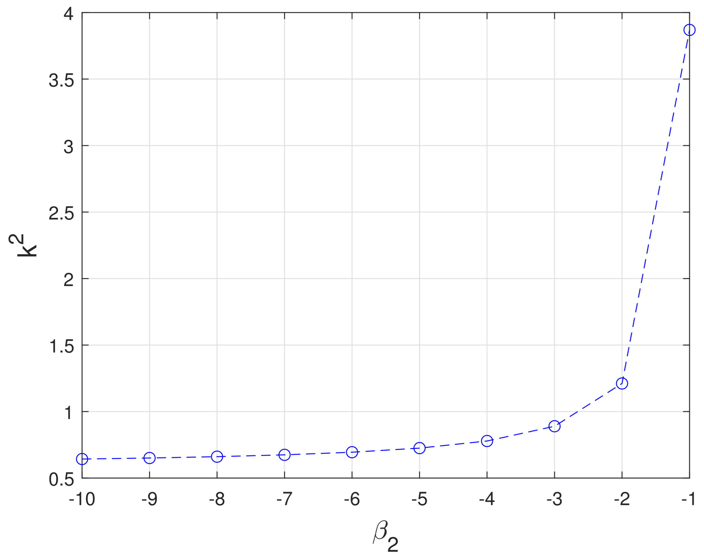
Figure 3.
Eigenvalues of (11) for different value of the wave number and when Also, , , , , and .
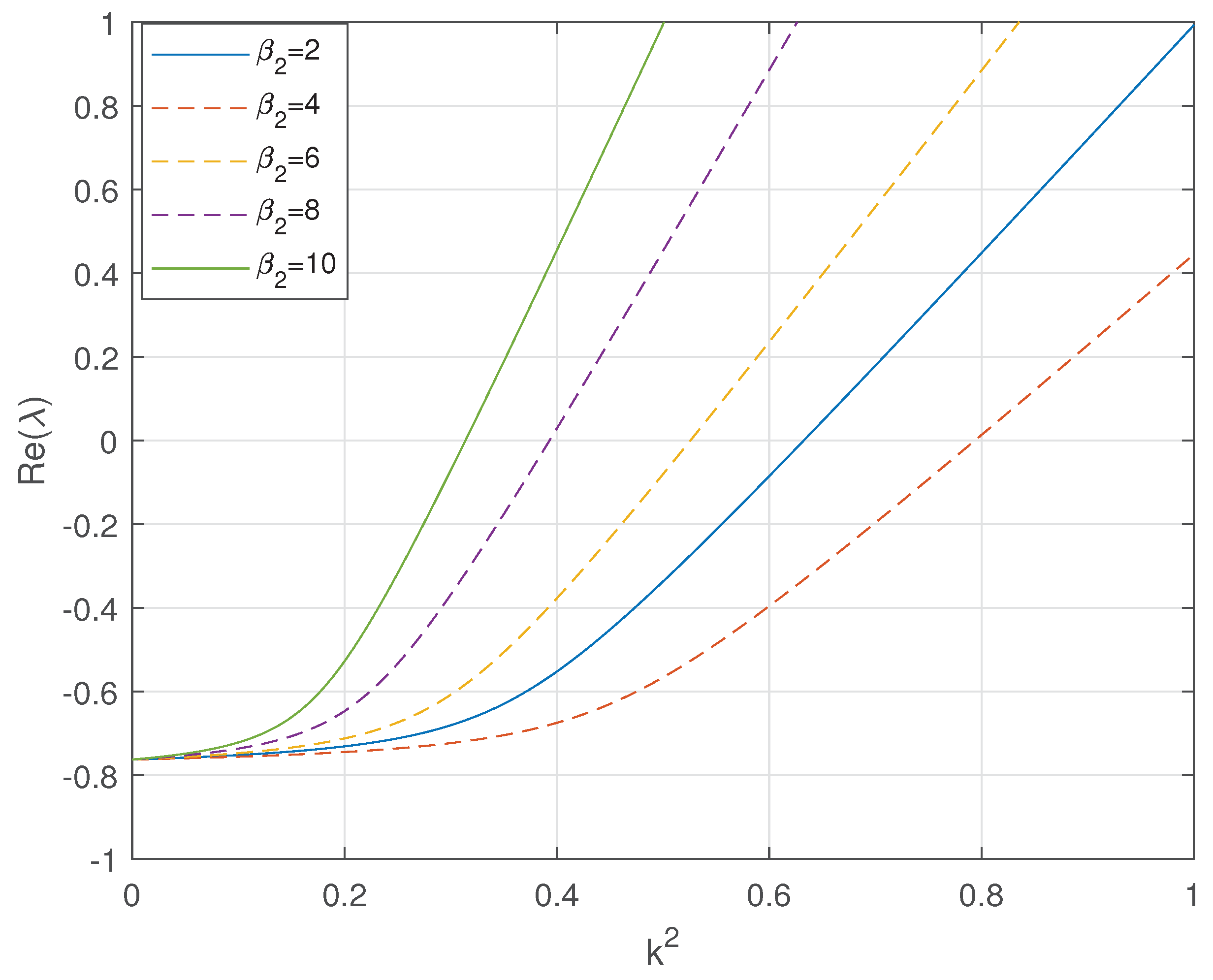
Figure 4.
The pattern formation for in the first column at the left and in the second column to the right. The first row represents the self-diffusion case, the second row represents the cross-diffusion case.
Figure 4.
The pattern formation for in the first column at the left and in the second column to the right. The first row represents the self-diffusion case, the second row represents the cross-diffusion case.

Figure 5.
The pattern formation for non-linear diffusion, the first column to the left is and the second column to the right is . has been in the first row to be positive and in the second row is positive. Patterns emerge with negative coefficients modeling repulsive interactions in crystal lattices [36].

Disclaimer/Publisher’s Note: The statements, opinions and data contained in all publications are solely those of the individual author(s) and contributor(s) and not of MDPI and/or the editor(s). MDPI and/or the editor(s) disclaim responsibility for any injury to people or property resulting from any ideas, methods, instructions or products referred to in the content. |
© 2025 by the authors. Licensee MDPI, Basel, Switzerland. This article is an open access article distributed under the terms and conditions of the Creative Commons Attribution (CC BY) license (http://creativecommons.org/licenses/by/4.0/).
Copyright: This open access article is published under a Creative Commons CC BY 4.0 license, which permit the free download, distribution, and reuse, provided that the author and preprint are cited in any reuse.


