Temporal Changes in Tropical Forest Plant Habitats After a Severe Tropical Cyclone, with and Without the Effects of Fire

Daniel Collins

doi:10.20944/preprints202508.1983.v1

Submitted:

26 August 2025

Posted:

27 August 2025

You are already at the latest version

Abstract

The forests of the tropical lowlands between Cairns and Ingham in North Queensland are among the most biodiverse and complex ecosystems in Australia. They consist of a myriad of regional ecosystems inter-mixed and positioned into a patchwork mosaic that ranges from open tropical woodlands, to flooded forest types to closed forest types known as “Vine Forests” (Cumming, 1993). These forests are continually in a state of change, regenerating from severe disturbances such as tropical cyclones, floods and fire events. This area was struck by severe tropical cyclone Yasi in early 2011. 31 plots estab-lished in the lowlands of the wet tropics after the cyclone, additional factors of influence to fire were added to the study, with approximately half the plots being treated with fire in the years that followed. All plots were then resurveyed in 2014. It was found that the fires promoted Acacia spp. stem density and this genus was significantly linked to higher fire frequency and scorch height. In terms of the effects of the cyclone, there were abundant woody plants in the ground layer following the cyclone, and this may also have been encouraged further by the fires, although that combined effect was not con-clusive. Across all forest types, numbers of ground plants were significantly more abundant with increasing distance from closed forest patches in the initial surveys. In the final survey greater ground plant species richness was significantly linked to increasing distance from closed forest. There was a significantly greater number of ground plants in the final survey. Most of the very large trees survived, while some trees throughout the tree layers died slowly over a year or more after the cyclone. The mean height and di-versity of all tree species combined increased significantly by the final data survey. Ultimately the forest was changed but survived.

Keywords:

open forest

;

closed forest

;

rainforest

;

cyclone

;

fire

;

DBH

;

height and diversity

Subject:

Environmental and Earth Sciences - Ecology

1. Introduction

The forests of the tropical lowlands between Cairns and Ingham in North Queensland are among the most biodiverse and complex ecosystems in Australia. They consist of a myriad of regional ecosystems inter-mixed and positioned into a patchwork mosaic that ranges from open tropical woodlands, to flooded forest types to closed rainforest types known as “Vine Forests” (Cumming, 1993). These forests are continually in a state of change, regenerating from severe disturbances such as tropical cyclones, floods and fire events. The mosaic is constantly in a state of change, and the types of forest also change over time.

The severe tropical cyclone event “Yasi” in February 2011, which crossed the coast between Cairns and Ingham provided a great opportunity to study the effects of disturbance in these forest types. It has been calculated by the Bureau of Meteorology that Yasi was a borderline category 4 – 5 cyclone (Turton, 2019). It has been claimed by Jonathon Nott (JCU) however, that Yasi with maximum wind gusts of up to 295km per hour, may have been a one in 200 or even 300-year event and concluded that climate change may and probably is causing less frequent but more severe cyclones (Was Yasi Australia’s Biggest Cyclone, ABC, 2011).

Understanding what drives these changes within a forest community, can be explained by a range of independent variables. The “Core Variables” used in this study may be linked to the resultant plant species growth, survivorship and distribution, such as time since previous burn, burn frequency and light penetrating through the canopy. It was important to ascertain how the forest communities change after disturbance. A wide range of environmental factors also influence which trees and smaller plants grow, where they grow, and in what communities in the research area. It was also important to investigate the different forest strata because each vegetation layer includes a different composition of plants that contribute to the overall diversity of the forest and provide habitat for animals. Cyclones are a major disturbance that can open space in the canopy with impacts on all vegetation layers, whereas species in the ground and shrub layers are more likely to be impacted by fire events.

2. Methods

31 plots were established and covered a wide range of regional ecosystems and vegetation types, with a mosaic of woodlands, open forests and closed forests (see Table 1 in Appendix). There was also the additional influence of wildfires in the years following the cyclone, although these are believed to have missed the study plots. There were several controlled fires undertaken in the area in August and September 2011, plots burnt in those fires include plots 1, 2, 6, 7, 8, 9, 14, 15, 22 and 23. All of these plots were established in July 2011, prior to being burnt. Plot 30 “Fishers Creek” received a wildfire in June 2011 but wasn’t established as a plot until 2012. Plot 15 “Conn Creek” was only burnt on the edges, but the fire did not intrude into the interior of the plot, primarily because it was such thick rainforest. The remaining burns were undertaken in 2012. The majority of the 31 plots were established and surveyed in 2011, and all 31 plots were resurveyed in 2014.

Plots left unburnt were also of value, and the overall influence of the cyclone, absence of fire and plots treated with fire made for an interesting study.

The overall rationale was based on a set of fire burn-offs in half the plots, and the other half left as controls. It was intended that the same variety of different levels of rainforest regrowth would be burnt as would be left unburnt among the plots. Therefore, there would be two sets of before and after results that were obtainable: burnt and unburnt, with approximately the same number of plots (15) across low, medium and high levels of rainforest regrowth. Furthermore, any recommendations that could be made for management of these forests was a central outcome intended from this study.

With the standard Queensland Herbarium CORVEG (Neldner et al., 2019) data that was taken, there were some slight modifications made to suit this research project. Plots were shortened in length to 20m x 20m quadrats. Also, grasses and ground covers were in most cases counted rather than estimated in % cover. Where % cover was used to estimate plants in the ground layer it was still converted to the best relative estimated number, and this was particularly so with densely grouped species such as Imperata spp.

The main aim of the study was to test whether there were compositional or structural changes in the plant communities, from the beginning of the study (initial survey shortly after the cyclone) to the end of the study (final survey three years after the cyclone), within the different strata of the forests, and whether these changes were influenced by the cyclone, treatment (burning or non-burning), forest type and/or also possibly climate change.

3. Statistical Analysis

Regressions were used to calculate basic correlations and significant relationships. In the more advanced analyses PRIMER7 was used. For the effects of survey period and fire two factor permutational Analysis of Variance was used in PRIMER v7 + PERMANOVA was used. For univariate analysis Euclidean distance similarly matrices were generated, whereas for the multi-variate analysis of plant community composition, Bray-Curtis similarity matrices were generated on the square-root transformed abundance data. In all cases 9999 permutations were run with unrestricted permutation of the raw data. To further investigate the effects of forest type, a four factor PERMANOVAs was used with survey period and fire treatment, as well as wet vs dry forest and forest type (four levels nested in wet vs dry). Shannon’s Diversity Index was used within PRIMER7 to assess tree layer diversity. PERMANOVA analyses were used to provide tables showing lists of individual species composition and similarity of % in varying forest types and under different treatments.

4. Results

4.1. Ground Layer

In the ground layer an outstanding result was the significant increase in species richness, between the initial survey and the final survey (P=<0.05).

Figure 1. Difference in ground plant species richness across treatments with median, second quartile, standard deviation and outliers, data grouped for burnt and unburnt plots in the initial and final survey.

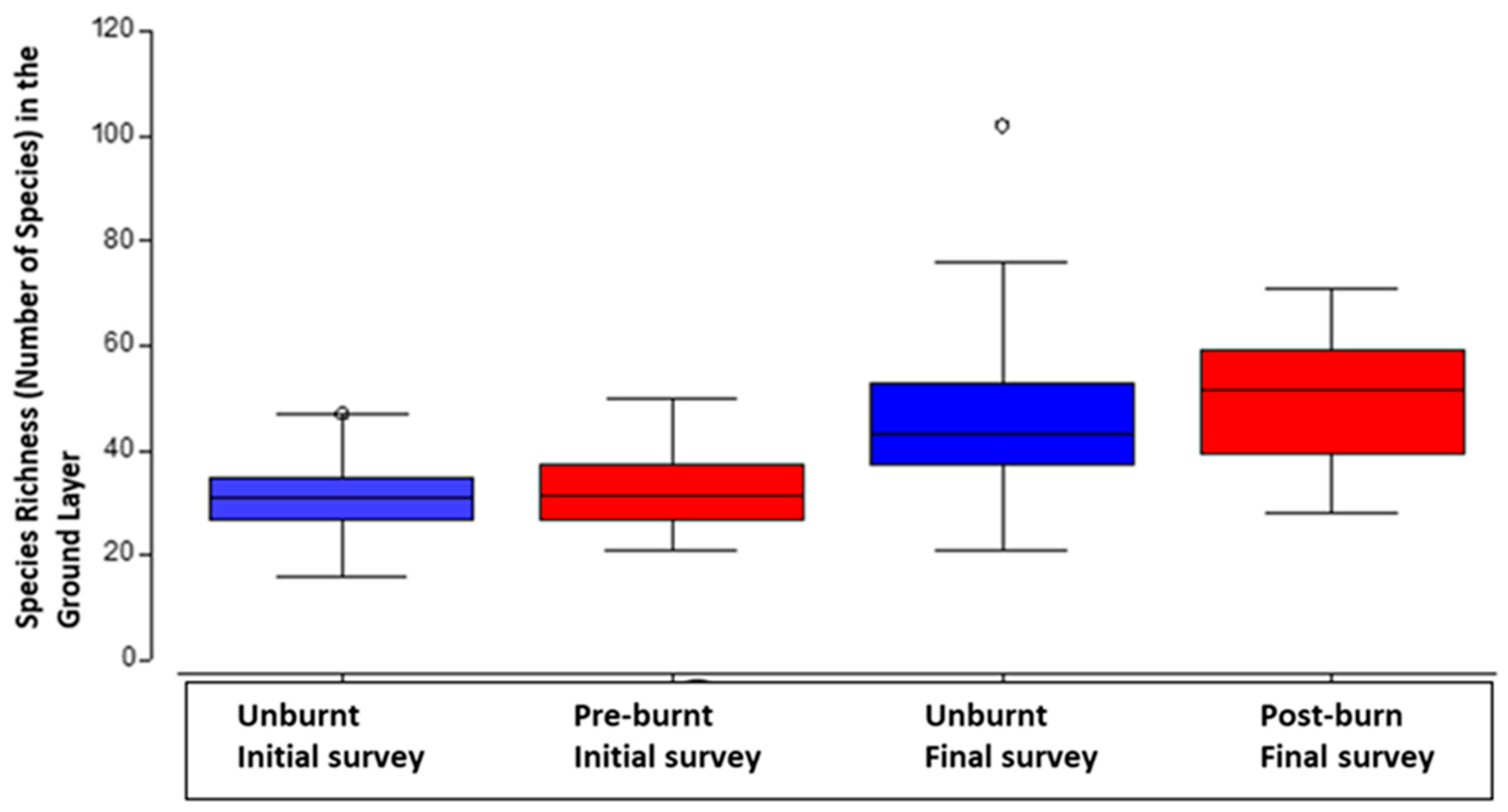
Table 1. Permutational ANOVA: difference in ground plant species richness between initial and final survey, across all plots both treated and untreated. Unrestricted permutation of raw data.

Source	df	SS	M	Pseudo-F	P (Perm)	Unique Perms
Treatment	1	62.842	62.84	0.41	0.53	9604
Survey	1	4261.4	4261.4	27.83	0.0001	9812
Treat x Survey	1	8.092	8.09	0.05	0.83	9815
Residual	58	8882.4	153.15
Total	61	13231

In the ground layer another outstanding result was the significant increase in the number of plants, between the initial survey and the final survey (P=<0.05). There were significantly more numbers of ground plants in the final burnt plots.

Figure 2. Comparison in ground layer plant abundance according to survey and treatment type (burnt or unburnt) with median, second quartile, standard deviation and outliers. .

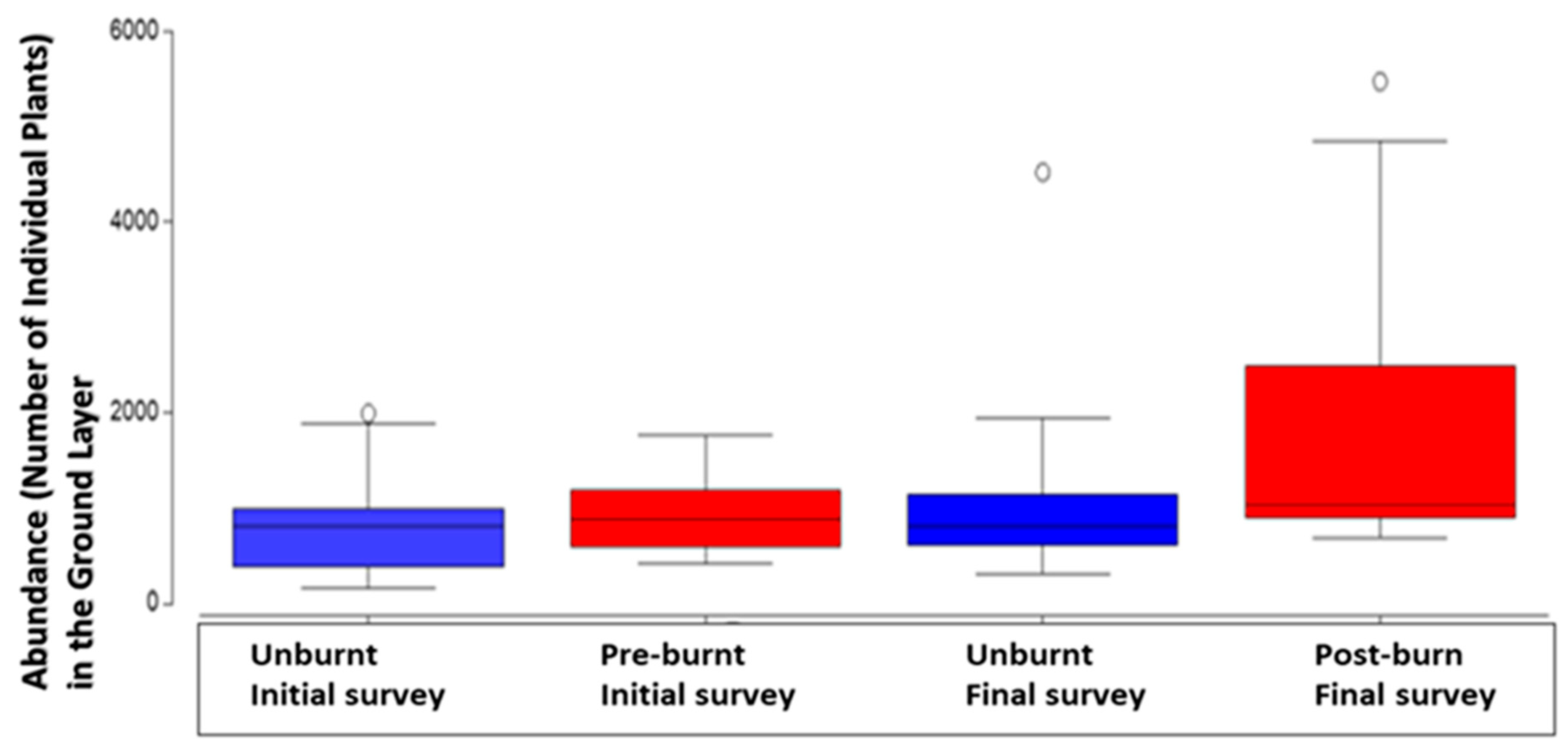
Table 2. Permutational ANOVA: difference in ground plant abundance between initial and final survey, across all plots both treated and untreated. Unrestricted permutation of raw data.

Source	df	SS	MS	Pseudo-F	P (Perm)	Unique Perms
Treatment	1	3.05E+06	3.05E+06	3.55	0.06	9849
Survey	1	5.50E+06	5.50E+06	6.41	0.01	9826
Treat x Survey	1	9.10E+05	9.10E+05	1.06	0.32	9819
Residual	58	4.98E+07	8.59E+05
Total	61	5.94E+07

There was a significant relationship between distance from closed forests and the number of ground plants in the initial survey data (P<=0.05, Table 3a). The total number of ground plants increased significantly with increasing distance from closed forest patches (Figure 3a). It was the number of species per plot that was significantly different for the final survey data three years after the cyclone, with significantly higher numbers of species (species richness) (P=<0.05) (Table 3b & Figure 3b).

4.2. Shrub Layer

In the shrub layer an outstanding result was the significant increase in species richness, between the initial survey and the final survey (P=<0.05). There was significantly higher species richness in the final survey plots, especially the unburnt final survey plots.

There was no significant influence of fire on number of shrub layer plants.

Figure 4. Comparison in shrub species richness according to treatment (burnt or unburnt) during initial and final surveys, with median, second quartile, standard deviation and outliers. .

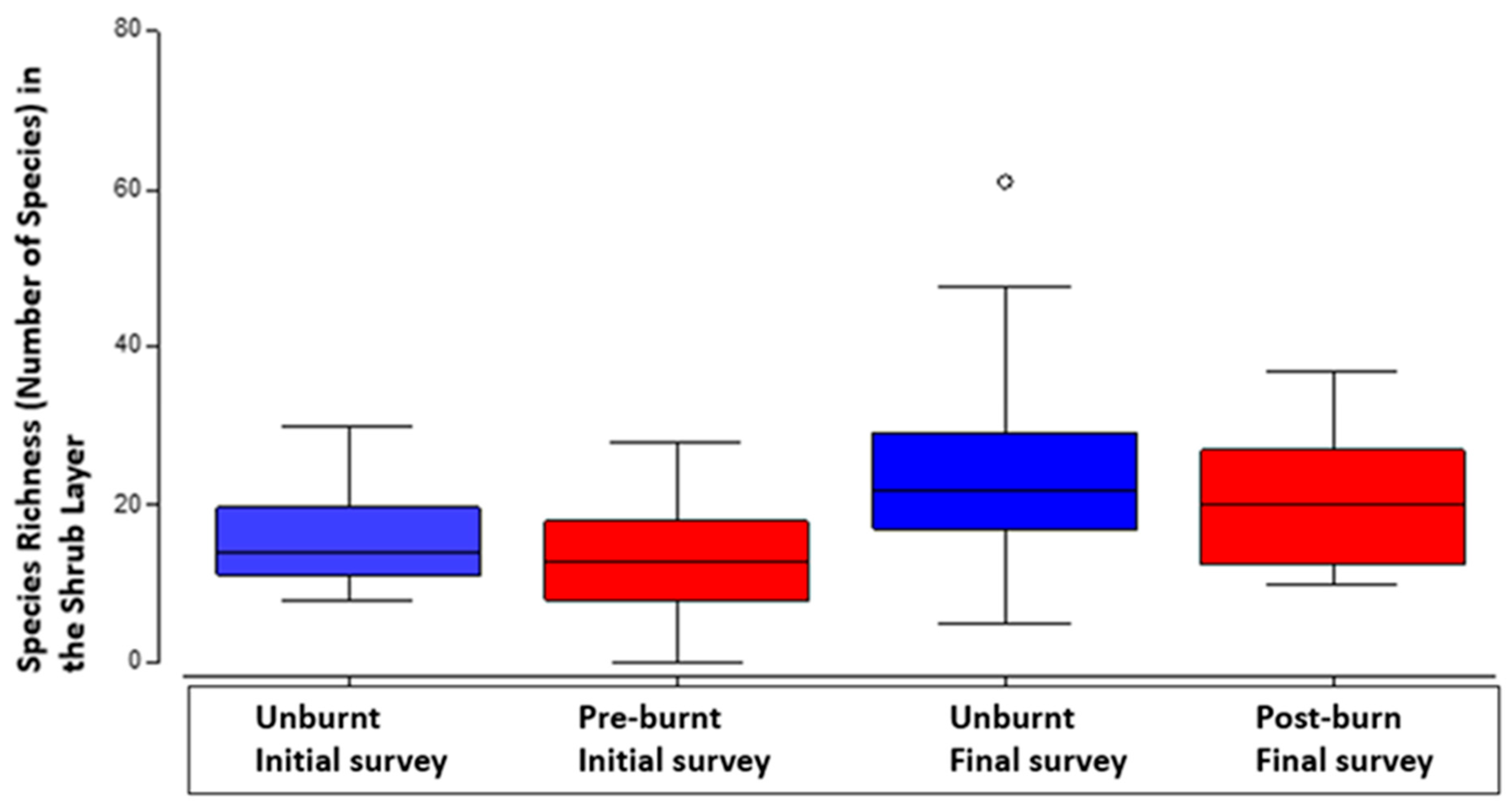
Table 4. Permutational ANOVA: testing the difference in overall shrub plant species richness between initial and final survey, and between treated (burnt) and untreated plots. Unrestricted permutation of raw databased on the Euclidean distance similarity matrix.

Source	df	SS	MS	Pseudo-F	P (Perm)	Unique Perms
Treatment	1	157.52	157.52	1.85	0.18	9386
Survey	1	930.5	930.5	10.92	0.001	9733
Treat x Survey	1	1.53	1.53	0.02	0.9	9774
Residual	58	4944.6	85.25
Total	61	6032.7

4.3. Tree Layers

There were 75 species of trees that were identified across all plots and both surveys. There were no significant effects of burn treatment or survey time between initial and final survey data on species richness in the tree layers. Three was a significant difference in the overall number of tree layer plants between unburnt and burnt plots. (P=<0.05, Table 5 & Figure 5). The other outstanding result in terms of fire treatment was the increase in median number of tree stems in unburnt plots and a decrease in the median number of stems in burnt plots, between the initial survey and the final survey (P=<0.05, Table 5 & Figure 5).

When a four factor PERMANOVA was used to investigate the effects of habitat type in tree abundance, the difference between burnt and unburnt plots was no longer significant. However, there was a significant difference in stem numbers between forest types, with significantly more tree stems in wet underlying landscapes, especially the swampy forest types and open forests with vine understory. Open forests with vine understory forest types had the highest median number of plants in the tree layers (P=<0.05, Table 5 and Figure 6).

Table 6. Four Factor PERMANOVA: Abundance of tree stems in all trees between initial and final survey, treated (burnt) and untreated (unburnt or control) plots, across different forest types and wet or dry landscapes. Unrestricted permutation of raw data. Bray-Curtis similarity +d. (D1 Euclidean).

Source	df	SS	MS	Pseudo-F	P (Perm)	Unique Perms	P(MC)
Treatment	1	3105.6	3105.6	7.01	0.12	4304	0.10
Survey	1	54.48	54.48	0.32	0.60	4317	0.61
Wet or Dry	1	1325.1	1325.1	0.58	0.34	6	0.52
Forest type W/D	2	4762	2381	3.89	0.04	9937	0.03
Treat x Survey	1	7.07	7.08	0.04	0.86	9853	0.85
Residual	46	28137	611.67
Total	61	44159

4.4. Diversity in the Tree Layers

Shannon’s diversity index revealed another significant interaction between forest type and burning (P=<0.05, Table 7a). There was a higher diversity of tree species in burnt plots and in open forest with vine understory with wet underlying landscapes (P=<0.05, Figure 7b).

Figure 7. a. Difference in tree layer plant diversity (Shannon’s diversity index) across basic forest types with median, second quartile, standard deviation. Initial and final survey combined.

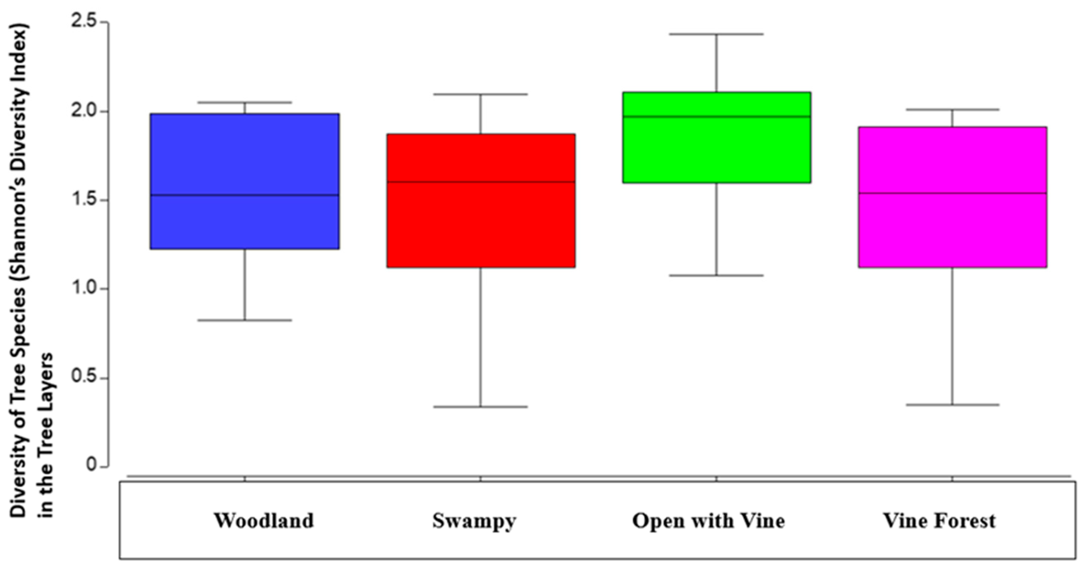
Figure 7. b. Difference in tree layer plant diversity (Shannon’s diversity index) between initial and final survey, across all plots both treated (burnt) and untreated (unburnt or control) plots, with median, second quartile, standard deviation and outliers. .

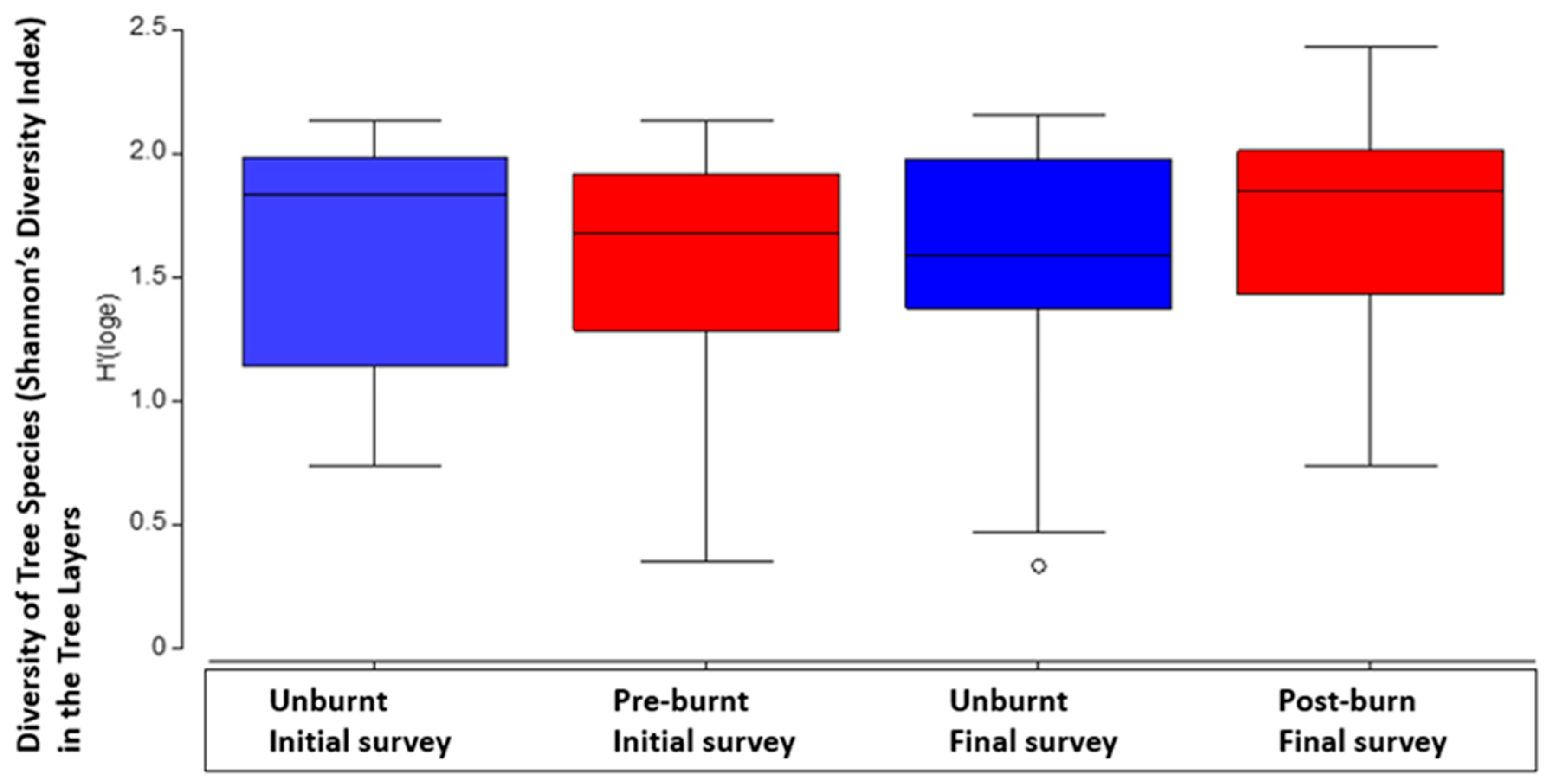
It is important to remember that diversity is different from species richness. Diversity incorporates species richness and the relative abundance of each species over the area.

4.5. Indicator Species in the Tree Layers

A Vector Overlay Analysis (Figure 8) revealed that despite significant differences between forest types, there was still a lot of variation in tree communities within forest types. Eucalyptus pellita and Lophostemon suaveolens were commonly associated with tree communities in swampy and open forest with vine understory. Melicope elleryana was more abundant in one subset of open forest with vine understory plots. Eucalyptus portuensis was associated with a variety of forest types but primarily in woodland forest types.

L. suaveolens featured strongly in the composition analyses for forest types (Figure 8) and was the most abundant tree species in the PERMANOVA analyses including when allowing for differences between burn and unburnt plots (Table 8). Eucalyptus pellita was often found in association with L. suaveolens. In particular, the average abundance of Lophostemon suaveolens drops markedly after the fire treatment. In fact, only Acacia spp., Melicope elleryana and Polyscias australiana increase in numbers after the fire treatments (Table 8). Corymbia clarksoniana was the second most abundant tree species. The Acacia’s, Acacia spp. were identified as a reliable indicator for burnt treated forest, with most often many times the number of trees in burnt plots compared to unburnt plots (Diss/SD >1, Table 8).

Further analysis of Acacia spp. and the influence of fire revealed that the critical interval that influences the growth of their trees was 5 years using a tree regression (Table 9 & Figure 9).

5. Discussion

The 3-year interval since the cyclone had the effect of increasing species richness in the ground layer in all final survey plots, but also of interest was that it was fire that increased the number of ground layer plants in the final survey in burn treated plots (Figure 1 & Figure 2). The higher median number of plants and species richness in these ground layer analyses was in the post burn treated plots, but it was survey interval that was the significant influence (P=<0.05, Table 1 & Table 2).

In the shrub layer, the higher median species richness was in the unburnt final survey plots, and the lowest median species richness was in the burn treated final survey plots (Figure 3). Fire decreases plant diversity in the shrub layer in these forests. There is a fundamental difference between the ground and shrub layers in that fire most influenced numbers of plants in the ground layer positively, while absence of fire influenced species richness positively in the shrub layer (Figure 4).

While time since the cyclone disturbance often leads to greater species, fire tends to lead to greater numbers of plants, particularly in the shrub and tree layers. In the tree layer fire increased stem density significantly, with an increase in the median stem density in unburnt plots and a decrease in median stem density in burnt plots, between the initial survey and the final survey (P=<0.05, Table 5 & Figure 5). Too much fire will thin the forest significantly. This is a key finding all fire managers need to realise when using fire in these forests in North Queensland.

In terms of diversity of species, there was a slightly different result. Diversity incorporates species richness and the relative abundance of these species over the area the species are found. In the tree layer, it was particularly interesting. It was clear that the open forest types with vine understories had the greatest diversity of tree species. The lowest diversity was found in the unburnt final survey plots (Figure 7 & Table 7). There was a combined significant influence of treatment, forest type and wet underlying landscape (P=<0.05, Table 7). It’s clear that fire is an important factor in managing these forests to maintain overall plant diversity. Without fire there is clearly a much lower diversity of plant species in these forests.

The highest tree species richness was found in open forest with vine understory, but an outlier in the vine forest type had a higher tree species richness than any other plot. This plot, “Deep Creek Hill”, a heavy rainforest lowland complex mesophyll vine forest. It was located in the base of the foothills midway between Tully and Cardwell. The forests in these ranges are sometimes known as “cyclone scrubs” (Webb, 1958), and more recent studies after Cyclone Larry in 2006, have shown that increased damage to trees leads to greater diversity and tree species richness, within rainforests and closed forest types (Murphy et al., 2013). The highest values for tree species richness in the final survey were clearly in the heavily rainforest invaded vine forest, Plot No. 23 “Deep Creek Hill”, regional ecosystem 7.12.1a: (“mesophyll to notophyll vine forest, on lowland granites and rhyolite”). This plot had the estimated longest time since fire of any of the plots, with an estimated 50 years since fire before its 2011 burn (Personal Comm. Parsons 2014). Although this was an outlier plot, this suggests absence of fire increases tree species richness in vine forests. (Table 1 in the Appendix).

In terms of actual species, several trees stood out as indicator species. In the open forests with vine understories, Melicope elleryana was an indicator species. It is a famous pioneer tree species in North Queensland and is particularly important as food for butterflies and other insect species. Its flowers and nectar are the favoured food of the Ulysses Blue Butterfly (Papilo Ulysses). The flowers and fruit are also very attractive to birds, Feather-tail Gliders and Ringtail Possums (Fern 2014). M. elleryana had the greatest increase in mean numbers after burn treatments after Acacia flavescens, with around 4.5 times as many plants in burnt plots (Table 8). Clearly where M. elleryana is abundant there has most likely been frequent or recent fire, particularly in the open forests with vine understories.

Eucalyptus pellita and Lophostemon suaveolens were together the most indicative tree species in the open forests and swampy forest types (Figure 8). Both of these species dropped markedly in number of tree stems in burnt plots (Table 8). It is clear that L. suaveolens is this most abundant tree of all in the study (Table 8). The most widely distributed tree species through the different forest types was Eucalyptus portuensis (Figure 7).

The most indicative tree species, in reference to the influence of fire, were the Acacia’s (Acacia spp). All Acacia spp. increased in burnt plots, especially Acacia flavescens with almost 13.5 times as many plants in the tree layers in the final survey burnt plots (Table 8). By far A. flavescens was the most outstanding indicator species in reference to fire, and wherever this species is seen in abundance in the tree layers, it is clearly an indication that there has been an abundance of fire in that area. Similar recent studies from the nearby Cardwell Range area showed clearly that the main Acacia species in this study (Acacia crassicarpa, A. flavescens and A. mangium) will readily regenerate in time from seed when subjected to fire and/or soil heat of approximately 80º Celsius for five minutes (Congdon et al., 2011). Acacia mangium has been proven to germinate at higher soil temperatures, with studies showing at between 100º - 140º Celsius it’s seed germination rate was between 60-86% (Saharjo and Watanabe 1997). When soil temperatures exceed approximately 120º Celsius, most native tree seeds die (Williams, et al. 2004).

The influence of burn interval and numbers of Acacia spp. tree stems was highly significant, with far greater numbers of stems after 5 years without fire (P=<0.05), Table 9 and Figure 9). There were almost 4.5 times as many Acacia spp. tree stems in plots unburnt for 5 years or more. This information suggests intervals less than 5 years will help minimise Acacia spp. tree stem growth. This also supports the recommended burn guidelines for most of the forest types in this study, of approximate burn intervals of between 2-5 years (Queensland Department of National Parks, Sport and Racing 2013).

The reality is that there is a patchwork mosaic of vine forest/rainforest types and open forests in the coastal lowlands of North Queensland. It is important to remember that the highest species richness in the tree layer was in a complex vine forest type plot (Plot 23) with the longest time since previous burn; 50 years. The balance of rainforest and open forest is critical, and we need to manage for both these 2 most basic forest types in the future.

Overall, the cyclone, or more accurately the time period since the cyclone (3 years) was more significantly influential on the growth, abundance and species richness of plants then the effects of fire, with some outstanding exceptions like plot 23. If similar category cyclones as Yasi increase in frequency, we can expect to see more of these characteristics in these forests. The most likely scenario in most predictions is that tropical cyclones may increase in severity but not frequency, especially in the south-west Pacific Ocean (Knutson et al 2010).

Further research into the distances between closed and open forest patches and how that can be managed to minimise the effects of climate change and still maintain the diversity of regional ecosystems and species would be a valuable addition to this study in the future.

Appendix

Table 1. Plot Forest Types, Regional Ecosystems, All Tree Layers Combined Species Richness and Abundance (Final Survey).

Plot No.	Forest Type	Regional Ecosystem	Species Richness	Abundance	Most Recent Fire Year
1	Open Forest with Vines	7.3.8a	4	43	2011
2	Woodland	7.2.11g	9	64	2011
3	Woodland	7.2.11g	6	19	2010
4	Swampy	7.2.11b	3	25	2009
5	Swampy	7.2.4d	8	32	2009
6	Open Forest with Vines	7.3.8a	11	137	2011
7	Open Forest with Vines	7.3.8a	9	86	2011
8	Open Forest with Vines	7.3.45c	9	73	2011
9	Swampy	7.2.4a	6	42	2011
10	Swampy	7.2.4a	11	64	2009
11	Swampy	7.2.4e	7	40	1997
12	Open Forest with Vines	7.3.44	4	39	2009
13	Open Forest with Vine	7.3.7a	10	74	1999
14	Open Forest with Vines	7.3.8a	7	115	2011
15	Open Forest with Vines	7.3.45c	14	131	1997
16	Open Forest with Vines	7.3.45c	12	110	2012
17	Swampy	7.2.4a	9	70	2012
18	Swampy	7.2.4a	6	27	2009
19	Swampy	7.2.4d	10	239	1997
20	Open Forest with Vines	7.3.45c	14	82	2012
21	Open Forest with Vines	7.3.7b	14	163	1994
22	Vine Forest	7.12.24a	5	49	2011
23	Vine Forest	7.12.1a	16	205	2011 & 50 yrs
24	Vine Forest	7.12.24a	3	49	2012
25	Open Forest with Vines	7.3.12a	13	159	1995
26	Vine Forest	7.12.5d	10	118	1994
27	Woodland	7.11.50a	4	75	2010
28	Vine Forest	7.12.5d	4	49	2012
29	Vine Forest	7.12.4e	6	76	2012
30	Swampy	7.2.4e	9	128	2011
31	Vine Forest	7.12.24a	3	50	2013

Note: from personal communication with and notes by Mark Parsons, 2014.

References

Cumming, R. J. (1993). Mahogany Glider habitat vegetation mapping. (Unpublished internal report). Queensland Department of Environment and Heritage.
Knutson, T., McBride, J., Chan, J. et al. Tropical cyclones and climate change. Nature Geoscience 3, 157–163 (2010). [CrossRef]
Murphy, T. H., Bradford, M. G., Dalongaville, A., Ford, J. A & Metcalfe, D, J. (2013) No evidence for long term increases in biomass and stem density in the tropical rainforests of Australia. Journal of Ecology, 101(6), 1589-1597.
Neldner, V. J., et al. (2019). Methodology for survey and mapping of regional ecosystems and vegetation communities in Queensland. Version 5.1. Queensland Department of Environment and Science and the Queensland Herbarium, Brisbane.
Parsons, M. (2014). Personal communication with Mark Parsons in the Hinchinbrook Channel area. Manager, Natural Assets Fire Management, North Queensland. 2014.
Saharjo, B. H., & Watanabe, H. (1997). The effect of fire on the germination of Acacia mangium in a plantation in South Sumatra, Indonesia. The Commonwealth Forestry Review, 76(2), 128–131. http://www.jstor.org/stable/42608797.
Fern, K. (2014). Tropical Plants Database, Ken Fern. tropical.theferns.info. 2021-11-15. <tropical.theferns.info/viewtropical.php?id=Melicope+elleryana>.
Turton, S. (2019). Reef to ridge ecological perspectives of high energy storm events in northeast Australia. Ecosphere Volume 10 (1), e02571.10.1002/ecs2.2571.
Queensland Department of National Parks, Sport and Racing (2013). Planned Burn Guidelines, Wet Tropics Bioregion of Queensland. Queensland Parks and Wildlife Service.
Was Yasi Australia’s biggest cyclone? (2011, February 7). ABC Science. https://www.abc.net.au/science/articles/2011/02/07/3132144.htm.
Webb, L. (1958). Cyclones as an ecological factor in tropical lowland rain-forest; North Queensland. Australian Journal of Botany, 6(3), 220 – 228.
Williams, P., Kimlin S., Anchen., G & Staier, E (2004). Post fire sprouting and seedling recruitment of Acacia ramiflora (Mimosocaceae) a threatened shrub of sandstone and granite healthy woodland in northern Australia. Proceedings of the Royal Society of Queensland. Volume 111, pages 103-105.

Figure 3. a. Regression showing the correlation between the distance from closed forest patches and number of ground plants in the initial survey data.

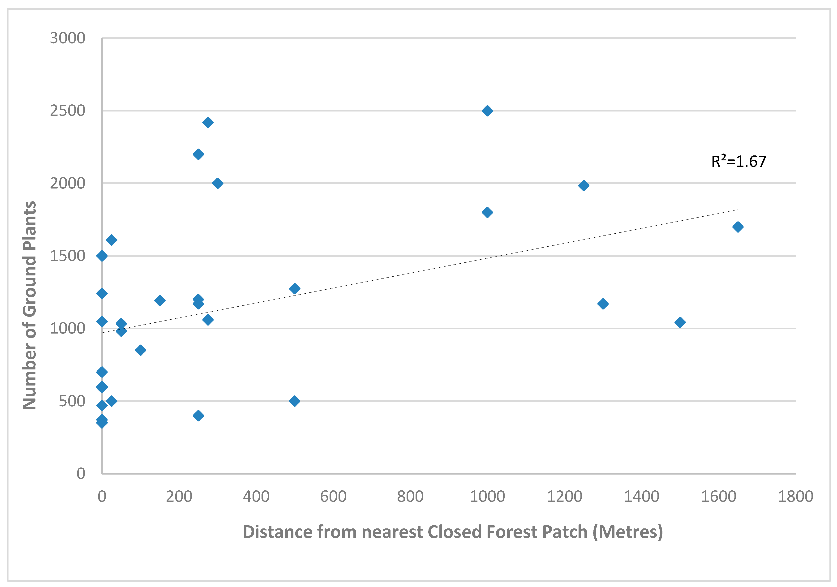
Figure 3. b. Regression showing the correlation between distance from closed forest patches and the number of ground plant species in the final survey data. .

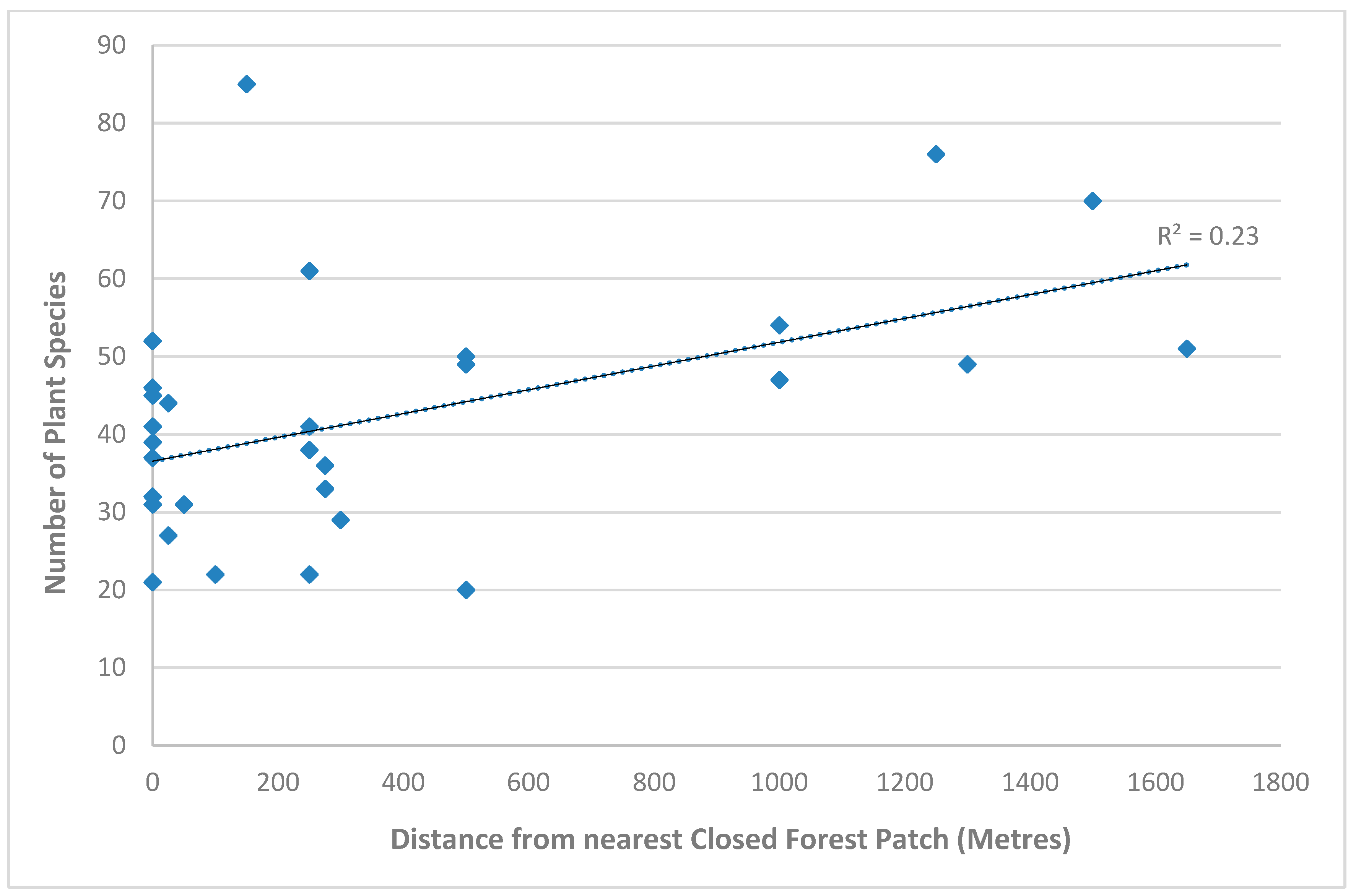
Figure 5. Comparison in tree layer plant abundance between initial and final survey, across all plots both treated (burnt) and untreated (unburnt or control) plots, with median, second quartile, standard deviation and outliers.

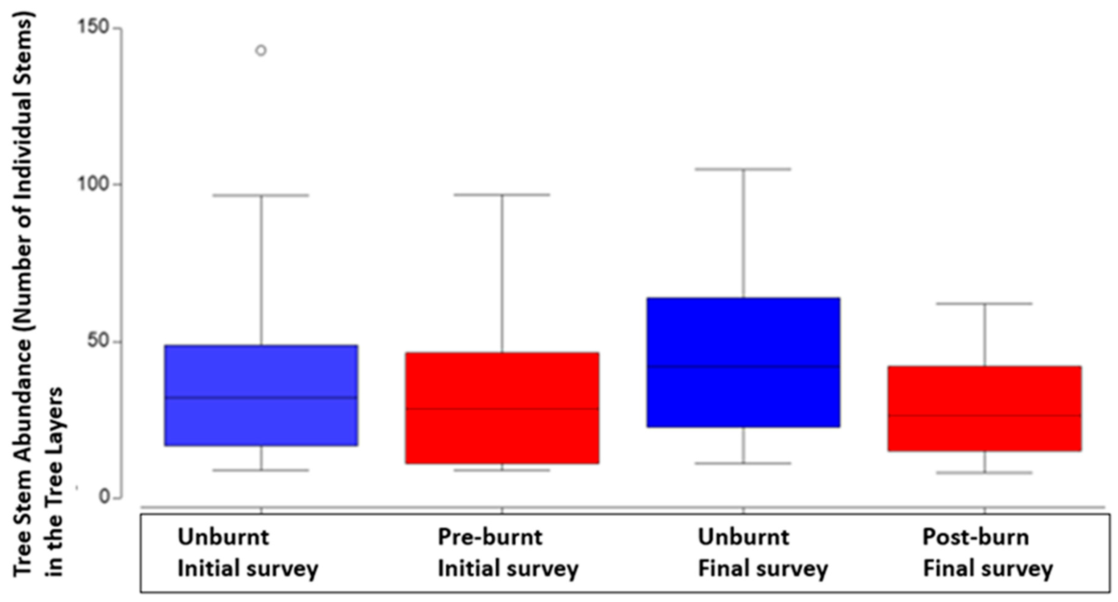
Figure 6. Difference in tree layer plant abundance across basic forest types with median, second quartile, standard deviation and outliers. Initial and final survey combined.

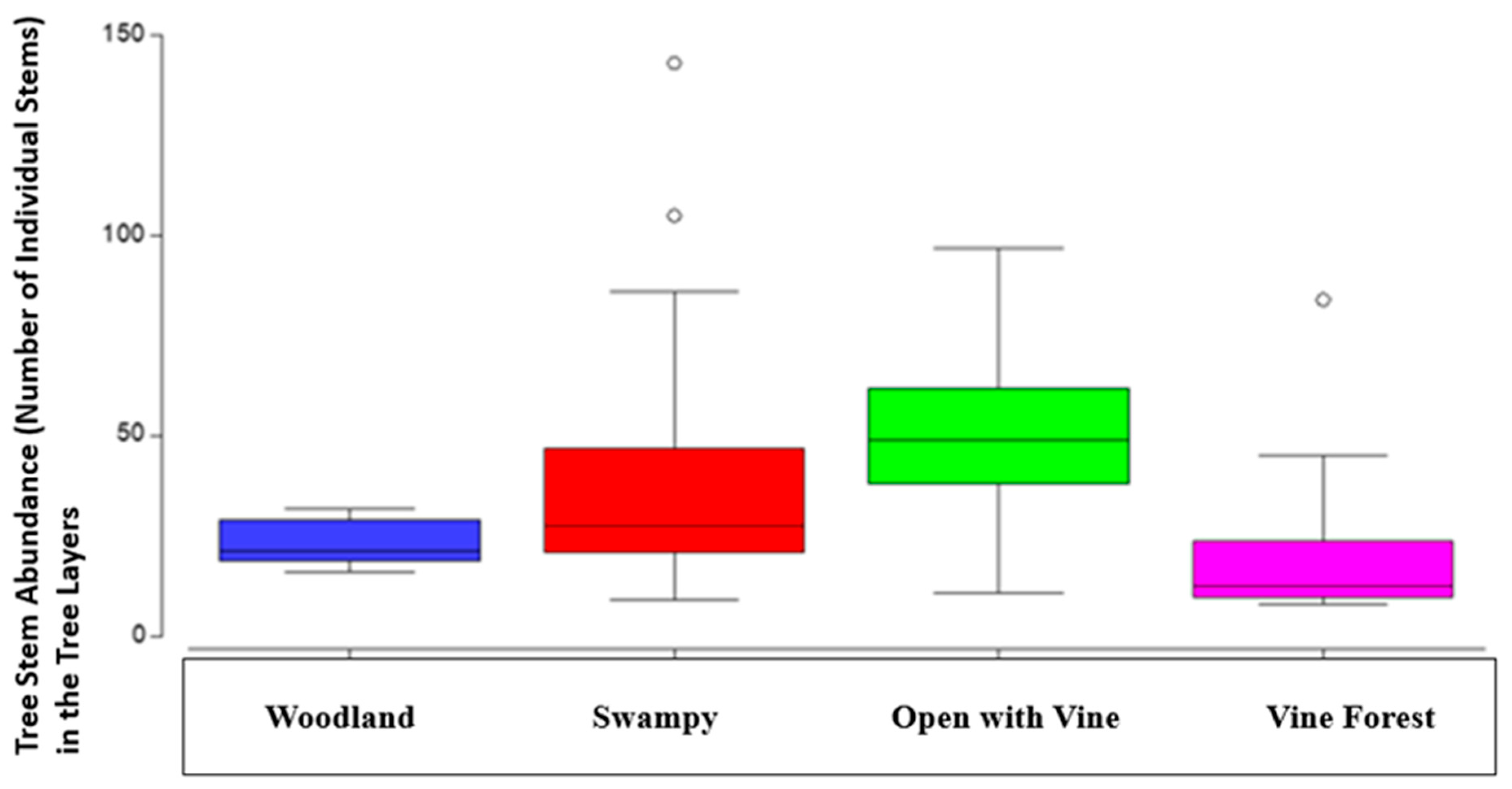
Figure 8. Tree species influencing the variation amongst basic forest type, across all plots, over both initial and final surveys, and burnt and unburnt plots. Vector overlay based on Pearson’s correlation > 0.6.

Figure 9. Regression Tree: Relationship between mean number of Acacia spp. stems per plot in the tree layers and burn frequency (number of years between burns), in a 5-year regime. Final survey data, all plots.

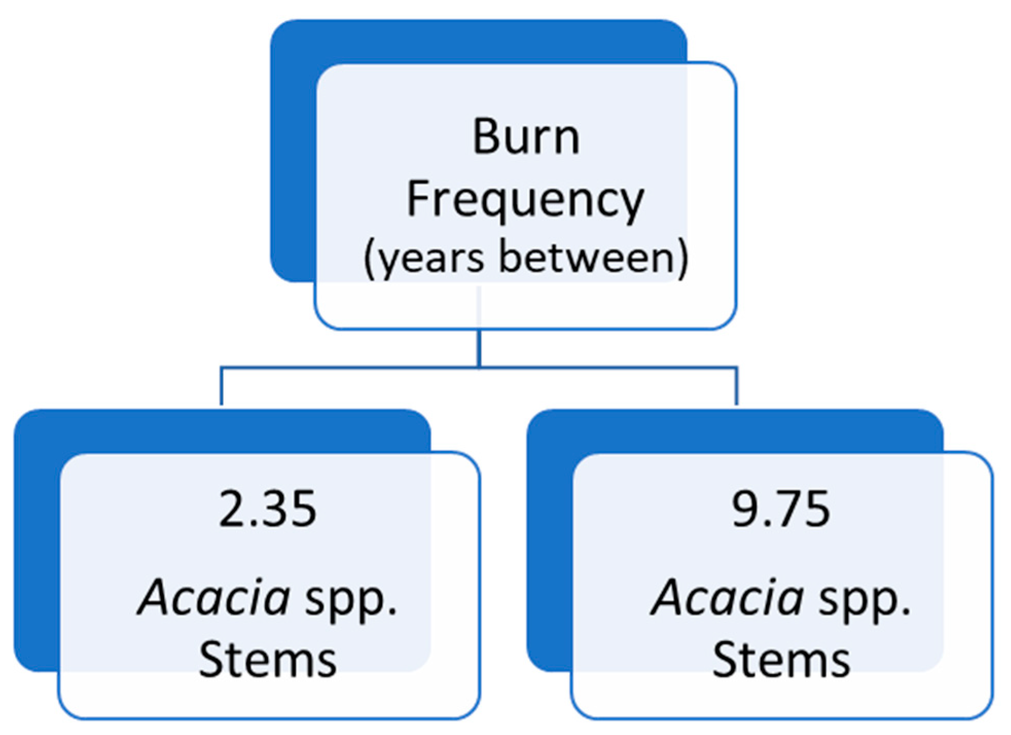
Table 3. a. Regression with linear results: main ground plant variables versus distance from closed forest patches (Initial Survey Data – All Plots).

DISTANCE FROM CLOSED FOREST: Regression Statistics			INITIAL SURVEY
Multiple R	0.51
R Square	0.26
Adjusted R Square	0.18
Standard Error	445.51
Observations	31
ANOVA	df	SS		MS	F	Significance F
Regression	3	1917042		639013.9	3.22	0.04
Residual	27	5358845		198475.8
Total	30	7275887
Main Ground Plant Data	Coefficients	Standard Error		t Stat	P- value
Intercept	-490.44	348.80		-1.41	0.17
No. of Ground Plants	0.32	0.13		2.46	0.02
Ground Mean Height	289.05	193.81		1.49	0.15
Ground Plant Species	10.25	9.42		1.09	0.29

Table 3. b. Regression with linear results: main ground plant variables versus distance from closed forest patches (Final Survey Data – All Plots).

DISTANCE FROM CLOSED FOREST: Regression Statistics			FINAL SURVEY
Multiple R	0.49
R Square	0.24
Adjusted R Square	0.15
Standard Error	451.06
Observations	31
ANOVA	df	SS		MS	F	Significance F
Regression	3	1687924		562641.4	2.77	0.06
Residual	27	5493245		203453.5
Total	30	7181169
Main Ground Plant Data	Coefficients		Standard Error		t Stat	P-value
Intercept	-349.94		300.03		-1.17	0.25
No. Ground Plants	0.09		0.23		0.39	0.70
Ground Mean Height	78.62		200.45		0.39	0.70
Ground Plant Species	14.54		5.58		2.60	0.02

Table 5. Permutational ANOVA: difference in tree layer plant abundance between initial and final survey, across all plots both treated (burnt) and untreated (unburnt). Unrestricted permutation of raw data. (D1 Euclidean).

Source	df	SS	MS	Pseudo-F	P (Perm)	Unique Perms
Treatment	1	2947	2947	4.16	0.04	9692
Survey	1	0.14	0.142	0.0002	0.99	9835
Treat x Survey	1	136.66	136.66	0.19	0.66	9827
Residual	58	41075	708.19
Total	61	44159

Table 7. Four factor permutational ANOVA: difference in overall tree diversity (Shannon’s diversity index) between initial and final survey, across all plots both treated and untreated, wet or dry underlying landscapes, and different forest types. Unrestricted permutation of raw data.

Source	df	SS	MS	Pseudo-F	P(Perm)	UniquePerms	P(MC)
Treatment	1	0.002	0.002	0.002	0.99	4335	0.97
Survey	1	0.04	0.04	3.42	0.22	4285	0.07
Wet or Dry	1	0.42	0.42	1.75	0.17	6	0.32
Forest (Wet/Dry)	2	0.48	0.24	1.19	0.31	9945	0.32
Treat x Survey	1	0.10	0.10	4.09	0.19	9861	0.10
Treat x Wet/Dry	1	1	0.08	0.07	0.86	4351	0.82
Survey x Wet/Dry	1	0.05	0.05	3.67	0.20	4265	0.06
Treat x Forest x Wet/Dry	2	2.30	1.15	5.67	0.006	9954	0.01
Survey x Forest x Wet/Dry	2	0.005	0.002	0.01	0.99	9942	0.99
Treat x Survey x Wet/Dry	1	0.03	0.03	1.25	0.39	9888	0.31
Treat x Survey x Forest x Wet/Dry	2	0.03	0.02	0.08	0.92	9952	0.92
Residual	46	9.30	0.20
Total	61	13.85

Table 8. Similarity of percentages showing abundances of all tree species in unburnt (control) and burnt (treatment) plots. Cut off for low contributions was 70%. One-way analysis.

PERMANOVA Table of Contents Average dissimilarity = 88.23
		Group: Unburnt	Group: Burnt
Species	Ave.Abund		Ave.Abund	Av.Diss	Diss/SD	Contrib%	Cum.%
Lophostemon_suaveolens		6.57	2.66	9.9	0.91	11.23	11.23
Corymbia_clarksoniana		2.5	1.41	4.96	0.68	5.62	16.85
Alstonia_muelleriana		3.93	1.41	4.94	0.65	5.6	22.45
Polyscias_australiana		1.97	2.91	4.78	0.54	5.42	27.87
Acacia_flavescens		0.2	2.69	4.09	0.69	4.64	32.51
Corymbia_intermedia		1.63	1.31	3.71	0.79	4.21	36.71
Litsea_leefeana		4.43	0.16	3.66	0.42	4.15	40.86
Eucalyptus_pellita		2.37	1.22	3.55	1.08	4.03	44.89
Syncarpia_glomulifera		2.47	0.03	3.41	0.27	3.87	48.75
Polyscias_elegans		2.03	1	3.4	0.53	3.85	52.61
Alpitonia_oblata		2.23	0.69	3.31	0.48	3.75	56.36
Melicope elleryana		0.43	2.22	3.12	0.61	3.54	59.9
Eucalyptus_portuensis		0.3	1	2.71	0.45	3.08	62.97
Acacia_mangium		0.87	0.91	2.69	0.48	3.05	66.02
Acacia_crassicarpa		0.53	1.72	2.63	0.57	2.99	69.01
Allocasuarina_torulosa		0.83	0.72	2.38	0.51	2.69	71.7

Table 9. Regression Tree Summary: Relationship between mean number of Acacia spp. stems per plot in the tree layers and burn frequency (number of years between burns). Final survey data, all plots.

Tree Regression Statistics Summary
	Plots	Deviance	Mean
Total Plots Tested	30	3.21	2.71
Burn Frequency: 5 years	15	4.20	2.35 – 9.75

Disclaimer/Publisher’s Note: The statements, opinions and data contained in all publications are solely those of the individual author(s) and contributor(s) and not of MDPI and/or the editor(s). MDPI and/or the editor(s) disclaim responsibility for any injury to people or property resulting from any ideas, methods, instructions or products referred to in the content.

© 2025 by the authors. Licensee MDPI, Basel, Switzerland. This article is an open access article distributed under the terms and conditions of the Creative Commons Attribution (CC BY) license (http://creativecommons.org/licenses/by/4.0/).

Copyright: This open access article is published under a Creative Commons CC BY 4.0 license, which permit the free download, distribution, and reuse, provided that the author and preprint are cited in any reuse.