Submitted:
26 August 2025
Posted:
27 August 2025
You are already at the latest version
Abstract
This paper presents an adaptive backstepping feedback control design for an unmanned aerial manipulator (UAM) which consists of an unmanned aerial vehicle (UAV) with attached robotic arm. The effect of the arm is treated as a disturbance force and torque to the UAV and as parametric uncertainty in the UAV inertial parameters. The proposed adaptive law guarantees disturbance rejection assuming constant parameters and disturbances. In practice, this assumption includes the case of fixed arm configurations. To validate the control design, numerical simulations are performed, where a realistic pick-and-place scenario is presented.
Keywords:
unmanned aerial vehicle (UAV)
; unmanned aerial manipulation (UAM)
; motion control
; stability analysis
1. Introduction
Research on unmanned aerial vehicles (UAVs) has recently focussed on tasks involving manipulation of the environment. Normally, this interaction is achieved by mounting an “arm” to the UAV so that various manipulation tasks can be achieved. The combined UAV and arm system is referred to as an unmanned aerial manipulator (UAM). Applications such as non-destructive testing of infrastructure require the UAM to keep a sensor in contact with the surface being inspected. The sensor must follow a desired trajectory on the surface and a predefined force must be applied.
Initial work on UAM motion control tends to focus on single-link arms which are rigidly attached to the UAV. UAM force and motion control dates back to [1], where the “arm” consists of a single rod rigidly attached to the UAV. An additional propeller is used to apply force to a surface. A heuristically designed proportional-integral-derivative (PID) controller structure is proposed, and no stability result is given for the force/motion control problem. Work in [2] provides a rigorous stability result using a nonlinear output feedback. The work assumes the single-fixed link arm does not affect the CoM of the system. The dynamics of the end-effector position is decomposed into tangential and normal directions. Error stability requires the beam to be attached "above" the UAV CoM. This work is extended in [3] where it is shown that the end-effector can generate any contact force if it is strictly located either below or above the UAV CoM. The article [4] studies the problem of UAV interaction with the environment without an arm. A’’ cascade controller allows the UAV to "push" against objects using pads attached to the UAV frame. The stability analysis is based on a planar quasi-static motion assumption. This apparatus is improved in [5] where tilted propellers are used. A heuristic PID control is proposed without a formal stability result.
Feedback control for multi-DoF arm UAMs can be classified into two main approaches: (i) separate controllers for the UAV and the arm, and (ii) full UAM control. In Approach (i), the coupling forces/torques acting on the UAV due to the arm are treated as a disturbance [6,7,8,9,10,11]. Approach (i) generally leads to a simpler subsystem-at-a-time design. Approach (ii) views the entire UAM as a single coupled dynamics [12]. This approach is challenging as the entire dynamics is very complex and complexity dramatically increases with the number of arm DoF [13,14,15,16,17]. Hence, this paper follows Approach (i) and compensates for the effect of the arm by introducing uncertain inertial parameters and force/torque disturbances into a UAV dynamics.
Approach (i) is widely found in the literature e.g., [6,7,8]. The work of [6] considers a UAV with a 4-DoF arm. For the UAV inner-loop, i.e., attitude dynamics, a disturbance observer based on [18] is used to estimate the effect of the arm on the UAV. With these estimates, feedback control is designed for the inner-loop that compensates for the disturbance. The outer-loop is treated separately. The effect of coupling between the loops on closed-loop stability is not considered. To validate their approach on a real UAM, the UAV outer-loop controller is taken from [19]. Work in [20] uses model reference control for the UAV outer-loop only. The UAV mass is taken as the unknown parameter. The effect of coupling forces and torques due to the arm on the UAV is not considered. Unlike [6] and [20], our work rejects the arm disturbance while considering the full UAV dynamics. The article [21] considers a UAV with a 3-DoF arm. It proposes a solution for constant setpoint regulation using a Luenberger observer to estimate the torque disturbance due to the arm. Our work is not limited to regulation and designs a trajectory-tracking feedback. We remark that the literature on robust UAV control, i.e., without an arm, is related to Approach (i). Examples of this include [22,23].
In this paper, our control objective is trajectory tracking of the UAV CoM and yaw. The effect of the arm on the UAV is modelled in two ways: it adds a force and torque disturbance to the UAV and introduces parametric uncertainty e.g., arm motion alters the UAV CoM and inertia matrix. We are inspired by the work of [24,25] on UAV motion control. These contributions only consider the force and torque disturbances, while all the inertial parameters are assumed known. Our work also allows for unknown inertial UAV parameters. We propose an adaptive backstepping control scheme that is capable of compensating force/torque disturbances and parameter uncertainty. This work is based on the first author’s thesis [26].
2. Modelling
Consider a UAM consisting of a UAV with attached robotic arm. In this section, we present the UAV model and introduce a force/torque disturbance and parametric uncertainty to model the effect of the arm. The UAV model neglects the effects of motor dynamics, rotor drag, and the rotor gyroscopic effects. The details on modelling these higher-order effects are discussed in [27,28].
Consider Figure 1. Let denote an inertial navigation frame with basis vectors pointing north, east, down, respectively. Let denote a body-fixed frame whose origin coincides with the UAV CoM and whose basis vectors are and point forward, right, and downward, relative to the UAV. The position of the origin of relative to the origin of is denoted, , which is expressed in . The linear velocity the UAV CoM, , is given by
The orientation of relative to is described by the rotation matrix . The angular velocity of the UAV relative to expressed in is related to R by
where
The UAV input is total propeller thrust which creates a force in direction, and torque on . Letting denote UAV mass and denote UAV inertia, the UAV dynamics is
where , , and g is gravitational acceleration. We remark that (3) models the UAV in isolation from the arm. To account for the effect of the arm, we introduce disturbance force and torque that can be interpreted as a change in input due to the arm. Further, we consider inertial parameters and J as uncertain:
Further details on the UAM model simplification are in [26] Section 2.2.4. 2.2.5.
Note that J in (Section 2) is a positive definite symmetric matrix with six unique entries. These entries of J define the vector . Using we can re-write the term in (4d) as
where . In model (Section 2) we take a, , and as unknown constants and denote , , , and as their estimates. Estimation errors are defined as , , , and .
3. Control Design
This section presents the control design for the UAM model (4). Figure 2 shows the structure of the proposed control, where the arm is controlled separately using a PID control. In this figure, we denote as the arm’s joint angles and their desired reference as . The proposed control compensates for the effect of the arm using an adaptive backstepping design method. The control objective is trajectory tracking for UAV CoM position p and UAV heading . We first present the design for tracking p and then extend it for tracking .
3.1. Position Tracking Control
Let represent the desired UAV CoM position and velocity, respectively. We define error coordinate. Taking its time-derivative gives
For this dynamics, consider the Lyapunov function . Taking its time-derivative gives
Adding and subtracting to , where is a controller gain,we obtain
From (7) we define so we can rewrite (6) as
Taking the time-derivative of , substituting the translational velocity dynamics from (4b), using , and , we arrive at
For the above dynamics, consider the Lyapunov function . Its time derivative is
In this expression, substituting for from (7) and for from (9), and simplifying, we arrive at
Adding and subtracting in the above equation, where is a controller gain we obtain
In the above equation, we define the coefficient of as
which can be rearranged as
Substituting this into (9) gives
The time-derivative of (11) is
Substituting (8) and (12) into the last equation, we get
Simplifying leads us to
For the above dynamics, consider the Lyapunov function whose time-derivative is
Substituting (13) in the last equation leads to
Adding and subtracting from the last expression, where is a controller gain, and simplifying gives
Now, consider a modified Lyapunov function
where are controller gains. The time-derivative of is
With some simplification, we get
We define to re-write (15):
Since is constant, we have . Substituting this equation in (15) and using the definitions of , we obtain
Adding and subtracting yields
and simplification gives
Observe
Hence,
Let’s factor out from the first three terms inside the parentheses of the coefficient and equate them to zero. In other words, let’s impose , which gives
Therefore,
The term in (19) can be interpreted as a virtual control, whose desired value is taken as
Since , the last equation can be rewritten as
Extracting individual components of , we have
while (19) becomes
Simplifying the last expression gives
Now, consider the following parameter update laws,
Substituting these adaptive laws in (23), we have
Let the error in angular velocity be . Using (4d), we can write
Define
Using instead of J, we have
where
Therefore, (26) can be rewritten as
Substituting and in (28) gives
Now, consider the Lyapunov function
where , are controller gains. Differentiating the above equation with respect to time gives
Substituting (25) and (29) into (31) gives
Let be a controller gain. Adding and subtracting in the above expression, factoring , we obtain
At this point, we assign the expression for input :
and define the parameter update laws
Substituting (34) and (35) in (33), and recalling that and are constants, we get
which is negative semi-definite.
Theorem 1.
Proof.
Consider the quadratic positive definite Lyapunov function in (30). According to [29] Lemma
4.3, there exist two positive definite functions that lower and upper bound . The time-derivative of after substitution of (34), (24), (35), is a negative semi-definite function. Using Barbalat’s lemma [29] Theorem 8.4, we can conclude as , and parameter and disturbance estimates , , and are bounded. Since is radially unbounded, we conclude that the equilibrium point is globally asymptotically stable. □
3.2. Position and Yaw Tracking Control
Thus far, the adaptive backstepping control design achieves trajectory tracking for p. Since the UAV has 4 control inputs, we can extend the control to track UAV heading, which is practically relevant for manipulation tasks. We identify UAV heading with yaw angle . Let the desired UAV yaw trajectory be and define tracking error . Let
Thus,
It can be computed that , where for 3-2-1 Euler angles parameterization, we have
and , represent UAV pitch, roll, respectively. Therefore, we can write
Adding and subtracting , where is a control gain, gives
Define
which gives
where is given in (22). Substituting (39) in (38) results in
We are now ready to state the stability result for the position-yaw tracking controller.
Theorem 2.
Proof.
Consider the Lypunov function with time derivative
Substituting for using (33), using parameter update laws (35), and the expression for in (41), gives
Substituting (42) gives
which is negative semi-definite. As in the proof of Theorem 1, we conclude as and parameters remain bounded. □
Remark 1.
The controllers presented in (34) and (42) depend on , however, the above derivation gives expression for . The value of can be obtained numerically by low-pass filtered finite difference. The algebraic expression for depends on which is not known. As well, the unknown inertia vector in the angular velocity dynamics makes the stability result difficult to prove. Work in [26] provides further details for alternate solutions to this problem.
4. Simulation Results
This section presents numerical simulations using MATLAB Simscape Multibody to validate our control design. The files to generate these simulations can be found at https://github.com/ANCL/UAM_control. A multibody simulation is necessary to avoid the complexity of simulating the closed-loop in a traditional state-space format. The UAM used in the simulation is shown in Figure 3. The arm is a 3-link 2-DoF manipulator with two revolute joints. Link 1 is attached to the CoM of the UAV and rotates in the plane about the origin of . Link 2 is a revolute joint which also rotates in the same plane. Link 3 is fixed to Link 2 and acts as a payload mass. The arm parameters are given in Table 2. The UAV parameters are given in Table 1. We consider three simulations: a figure-8 desired position with fixed and moving arm cases, and a pick and place operation.

Table 1.
UAV parameters.
| Parameter | Value | Parameter | Value |
|---|---|---|---|
| m | 1.6 | , | 0.03 |
| 0.05 | , , | 0.0 |
Table 2.
Arm parameters.
| Parameter | Link 1 | Link 2 | Link 3 |
|---|---|---|---|
| Joint Type | Revolute | Revolute | Fixed |
| Mass () | 0.1 | 0.1 | 0.1 |
| Length () | 0.2 | 0.3 | 0.1 |
| Inertia () |
4.1. Figure-8 Reference Trajectory
For the figure-8 trajectory, in addition to the coupling forces and torques due to the arm, we consider a constant external disturbance force of } acting at the UAV CoM. The controller gains used for all simulations are in Table 3. Initial conditions are , , and , , and i.e., we consider a 30% error in mass and a 40% error in inertia initially. The initial conditions for the disturbances are .
Figure 4a–f present the simulation results for the fixed arm case where the arm is locked in the direction. The position tracking errors in Figure 4b converge to a small neighbourhood of 0. Estimates , , , remain bounded. These estimates are shown in Figure 4c–e. We observe that in steady-state these parameters are time-varying due to the time-varying reference trajectory. That is, the UAV must vary its attitude to track the position trajectory, and this creates a time-varying disturbance. Increasing controller gains leads to faster tracking error convergence and smaller ultimate error bounds caused by time-varying disturbances.Figure 4f shows the control inputs.
The simulation results for the moving arm case are given in Figure 5a–f. The arm motion is taken as and . Figure 5b shows the UAV CoM position errors, which admit small oscillations around the origin. Relative to the fixed arm case, we observe larger error in steady-state. However, from a practical perspective, the error is not significant. The estimated parameters and disturbances are bounded and shown in Figure 5c–e. As in the fixed arm case, these parameters are time-varying in steady state, and large variations are observed. Figure 5f shows the control inputs.
We now present a practical pick and place motion where the UAM takes off to a target position, extends its arm, picks up a payload, flies to a desired location, and places the payload at the desired location. Multiple “table” landmarks are created in MATLAB Simscape Multibody that correspond to the various locations of the task. A small cubic payload of mass and dimension is attached to the end-effector. The UAV CoM start location is . The first and second desired UAV CoM positions and yaw are denoted Location 1 and Location 2, respectively. Location 1 is and Location 2 is , . When picking up the payload, the UAV position is lowered using a function . Table 4 shows the desired trajectory for the UAV and arm. The Home configuration for the arm is selected to be . The desired values of p and are shown in Figure 6a. The position errors are given in Figure 6b. The figures label each phase of the task. Evidently, the figures show tracking error is asymptotically convergent as expected by the theory. In this task, the assumptions of Theorem 2 hold as desired position and arm configuraiton is eventualy constant. Hence, this simulation case illustrates a practical case where assumptions hold.
5. Conclusion
In this paper, we have presented a control design for a UAM consisting of a UAV and multi-DoF robotic arm. The design is based on a UAV model that accounts for the arm’s effect by including torque and force disturbances and parametric uncertainty. An adaptive backstepping control law is presented that achieves UAV CoM position and yaw tracking when disturbances and parameters are constant. Numerical simulations demonstrate that bounded tracking error results when disturbances and parameters are varying. A practical pick and place task illustrates a case where tracking error converges. Future work involves indoor and output experimental validation of the control with an open source platform as in [30]. An intermediate step for this validation is software-in-the-loop testing that includes various non-idealities such as actuator saturation, sampling effects, state estimation, and rotor drag [31].
References
- Albers, A.; Trautmann, S.; Howard, T.; Frietsch, M.; Sauter, C. Semi-autonomous flying robot for physical interaction with environment. In Proceedings of the 2010 IEEE Conference on Robotics, Automation and Mechatronics, June 2010, pp. 441–446. [CrossRef]
- Nguyen, H.; Lee, D. Hybrid force/motion control and internal dynamics of quadrotors for tool operation. In Proceedings of the 2013 IEEE/RSJ International Conference on Intelligent Robots and Systems, Nov 2013; pp. 3458–3464. [Google Scholar] [CrossRef]
- Nguyen, H.N.; Ha, C.; Lee, D. Mechanics, control and internal dynamics of quadrotor tool operation. Automatica 2015, 61, 289–301. [Google Scholar] [CrossRef]
- Mersha, A.Y.; Stramigioli, S.; Carloni, R. Variable impedance control for aerial interaction. In Proceedings of the 2014 IEEE/RSJ International Conference on Intelligent Robots and Systems, Sep. 2014; pp. 3435–3440. [Google Scholar] [CrossRef]
- Papachristos, C.; Alexis, K.; Tzes, A. Efficient force exertion for aerial robotic manipulation: Exploiting the thrust-vectoring authority of a tri-tiltrotor UAV. In Proceedings of the 2014 IEEE International Conference on Robotics and Automation (ICRA), May 2014; pp. 4500–4505. [Google Scholar] [CrossRef]
- Kim, S.; Choi, S.; Kim, H.; Shin, J.; Shim, H.; Kim, H.J. Robust Control of an Equipment-Added Multirotor Using Disturbance Observer. IEEE Transactions on Control Systems Technology 2018, 26, 1524–1531. [Google Scholar] [CrossRef]
- Jimenez-Cano, A.E.; Martin, J.; Heredia, G.; Ollero, A.; Cano, R. Control of an aerial robot with multi-link arm for assembly tasks. In Proceedings of the 2013 IEEE International Conference on Robotics and Automation, May 2013; pp. 4916–4921. [Google Scholar] [CrossRef]
- Korpela, C.; Orsag, M.; Pekala, M.; Oh, P. Dynamic stability of a mobile manipulating unmanned aerial vehicle. In Proceedings of the 2013 IEEE International Conference on Robotics and Automation, May 2013; pp. 4922–4927. [Google Scholar] [CrossRef]
- Kannan, S.; Olivares-Mendez, M.A.; Voos, H. Modeling and Control of Aerial Manipulation Vehicle with Visual sensor. IFAC Proceedings Volumes 2013, 46, 303–309. [Google Scholar] [CrossRef]
- Kannan, S.; Alma, M.; Olivares-Mendez, M.A.; Voos, H. Adaptive control of Aerial Manipulation Vehicle. In Proceedings of the 2014 IEEE International Conference on Control System, Nov 2014, Computing and Engineering (ICCSCE 2014); pp. 273–278. [Google Scholar] [CrossRef]
- Khalifa, A.; Fanni, M.; Ramadan, A.; Abo-Ismail, A. Modeling and control of a new quadrotor manipulation system. In Proceedings of the 2012 First International Conference on Innovative Engineering Systems, Dec 2012; pp. 109–114. [Google Scholar] [CrossRef]
- Samadikhoshkho, Z.; Ghorbani, S.; Janabi-Sharifi, F.; Zareinia, K. Nonlinear control of aerial manipulation systems. Aerospace Science and Technology 2020, 104, 105945. [Google Scholar] [CrossRef]
- Lippiello, V.; Ruggiero, F. Exploiting redundancy in Cartesian impedance control of UAVs equipped with a robotic arm. In Proceedings of the 2012 IEEE/RSJ International Conference on Intelligent Robots and Systems, Oct 2012; pp. 3768–3773. [Google Scholar] [CrossRef]
- Lippiello, V.; Ruggiero, F. Cartesian Impedance Control of a UAV with a Robotic Arm. In Proceedings of the 10th International IFAC Symposium on Robot Control; 2012; pp. 704–709. [Google Scholar]
- Kim, S.; Choi, S.; Kim, H.J. Aerial manipulation using a quadrotor with a two DOF robotic arm. In Proceedings of the 2013 IEEE/RSJ International Conference on Intelligent Robots and Systems, Nov 2013; pp. 4990–4995. [Google Scholar] [CrossRef]
- Yang, H.; Lee, D. Dynamics and control of quadrotor with robotic manipulator. In Proceedings of the 2014 IEEE International Conference on Robotics and Automation (ICRA), May 2014; pp. 5544–5549. [Google Scholar] [CrossRef]
- Korpela, C.; Orsag, M.; Oh, P. Towards valve turning using a dual-arm aerial manipulator. In Proceedings of the 2014 IEEE/RSJ International Conference on Intelligent Robots and Systems, Sep. 2014; pp. 3411–3416. [Google Scholar] [CrossRef]
- Lee, K.; Back, J.; Choy, I. Nonlinear disturbance observer based robust attitude tracking controller for quadrotor UAVs. International Journal of Control, Automation and Systems 2014, 12, 1266–1275. [Google Scholar] [CrossRef]
- Bouabdallah, S.; Siegwart, R. Backstepping and Sliding-mode Techniques Applied to an Indoor Micro Quadrotor. In Proceedings of the Proc. IEEE Int. Conf. on Robotics and Automation. IEEE; 2005. [Google Scholar] [CrossRef]
- Baraban, G.; Sheckells, M.; Kim, S.; Kobilarov, M. Adaptive Parameter Estimation for Aerial Manipulation. In Proceedings of the Proceedings of the American Control Conference, 2020, pp. [CrossRef]
- Alvarez-Munoz, J.; Marchand, N.; Guerrero-Castellanos, J.F.; Tellez-Guzman, J.J.; Escareno, J.; Rakotondrabe, M. Rotorcraft with a 3DOF Rigid Manipulator: Quaternion-based Modeling and Real-time Control Tolerant to Multi-body Couplings. International Journal of Automation and Computing 2018, 15, 547–558. [Google Scholar] [CrossRef]
- Petrlík, M.; Báča, T.; Heřt, D.; Vrba, M.; Krajník, T.; Saska, M. A robust UAV system for operations in a constrained environment. IEEE Robotics and Automation Letters 2020, 5, 2169–2176. [Google Scholar] [CrossRef]
- Wang, Y.; Lu, Q.; Ren, B. Wind turbine crack inspection using a quadrotor with image motion blur avoided. IEEE Robotics and Automation Letters 2023, 8, 1069–1076. [Google Scholar] [CrossRef]
- Moeini, A.; Lynch, A.; Zhao, Q. Disturbance Observer-based Nonlinear Control of a Quadrotor UAV. Adv. Control Appl. 2019, 2, 1–20. [Google Scholar] [CrossRef]
- Moeini, A.; Rafique, M.A.; Xue, Z.; Lynch, A.F.; Zhao, Q. Disturbance Observer-Based Integral Backstepping Control for UAVs. In Proceedings of the 2020 International Conference on Unmanned Aircraft Systems (ICUAS); 2020; pp. 382–388. [Google Scholar]
- Rafique, M.A. Adaptive Nonlinear Control for Unmanned Aerial Vehicles: Visual Servoing and Aerial Manipulation. Ph.d. thesis, University of Alberta, Edmonton, Alberta, Canada, 2022. [CrossRef]
- Bangura, M. Aerodynamics and Control of Quadrotors. PhD thesis, College of Engineering and Computer Science, The Australian National University, 2017.
- Bouabdallah, S. Design and control of quadrotors with application to autonomous flying. PhD thesis, Ecole Polytechnique Federale de Luasanne, Lausanne, Switzerland, 2007.
- Khalil, H.K. Nonlinear Systems, 3 ed.; Prentice Hall: Upper Saddle River, NJ, 2002. [Google Scholar]
- Jiang, Z.; Yu, Y.; Lynch, A. Nonlinear Motion Control of a Multirotor Slung Load System: Experimental Results. In Proceedings of the American Control Conference (ACC); 2024; pp. 2851–2857. [Google Scholar] [CrossRef]
- Lawati, M.A.; Zhang, Z.; Yan, E.; Lynch, A.F. Nonlinear Control of a Multi-Drone Slung Load System. In Proceedings of the American Control Conference (ACC); 2025; pp. 1989–1996. [Google Scholar]
Figure 1.
Diagram of a quadrotor with modelling notation.
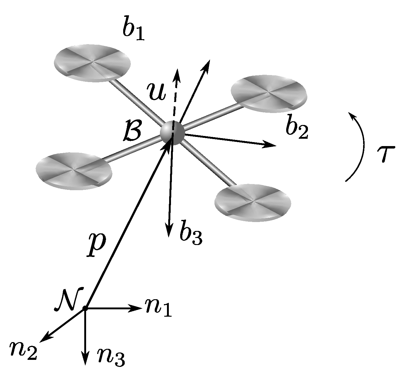
Figure 2.
The proposed UAM controller structure. The control of the UAV and arm are decoupled.
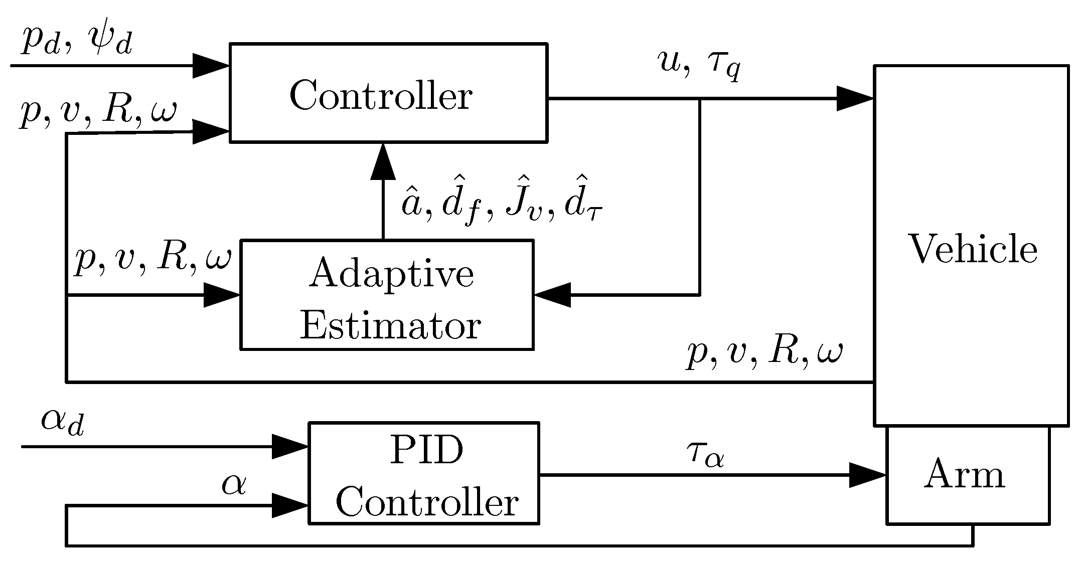
Figure 3.
UAM Configuration.
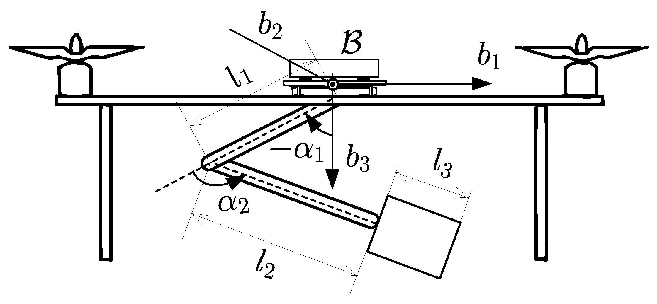
Figure 4.
Results for fixed arm configuration ().
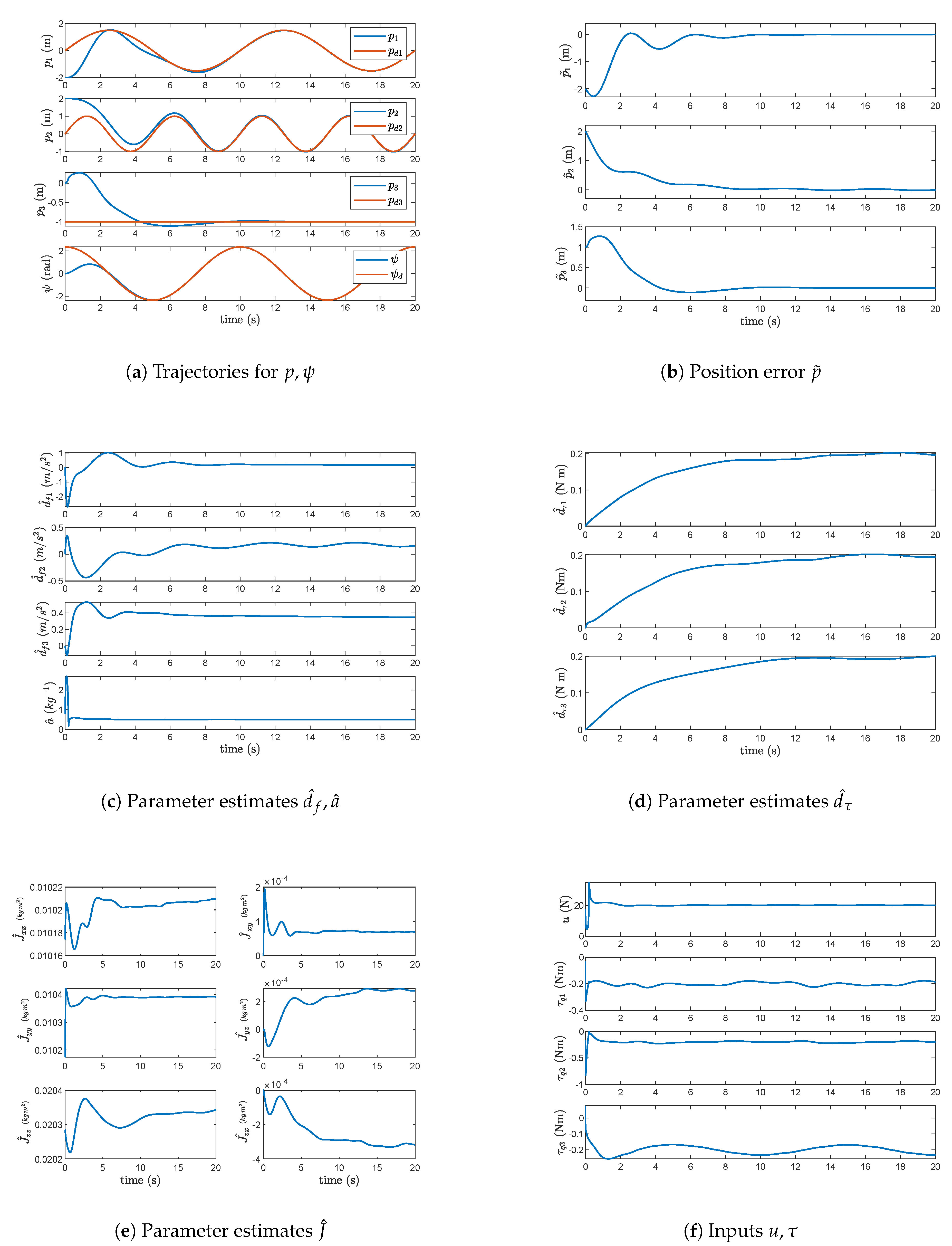
Figure 5.
Results for the moving arm configuration.
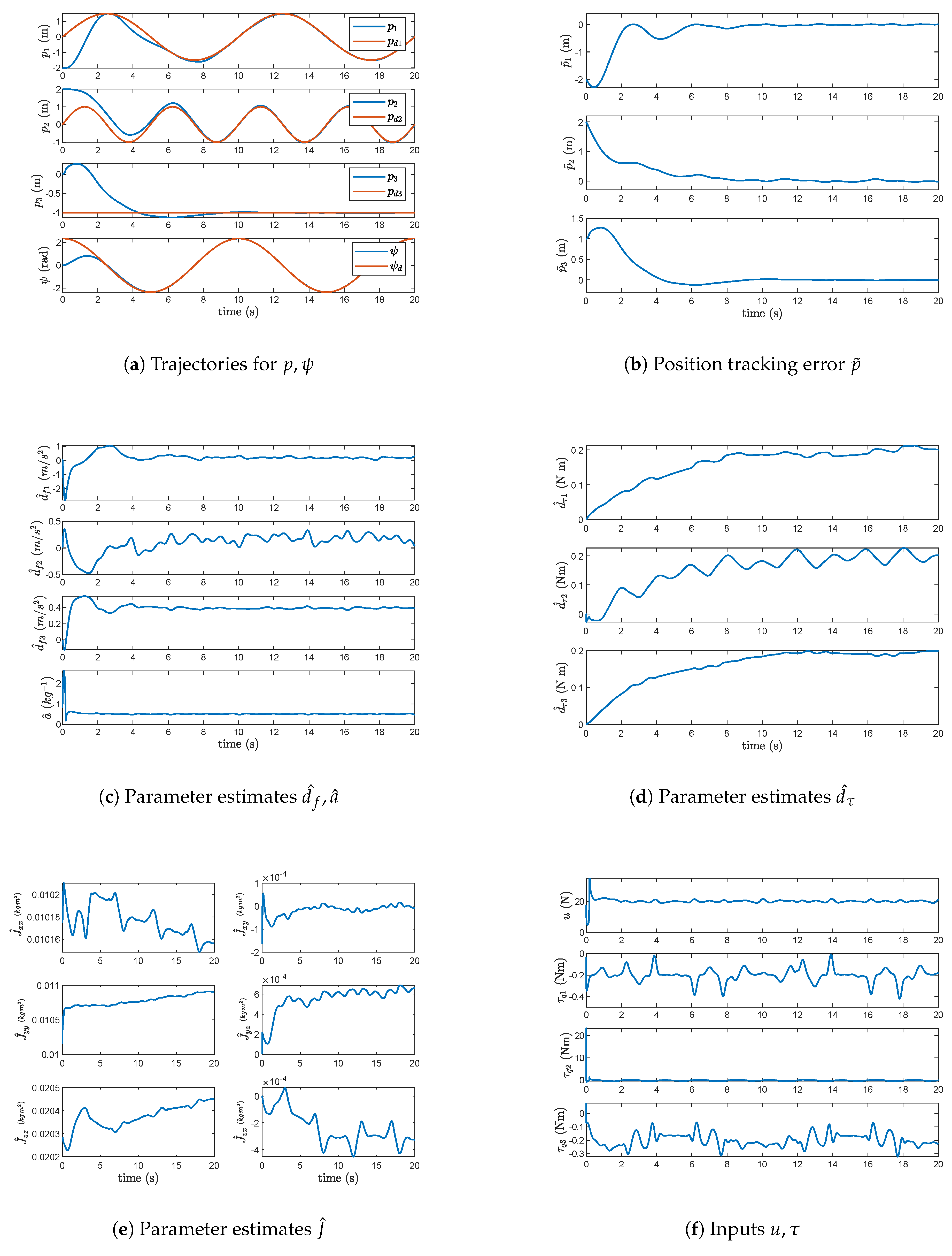
Figure 6.
Pick and place application results: (a) UAV pose and (b) position errors.
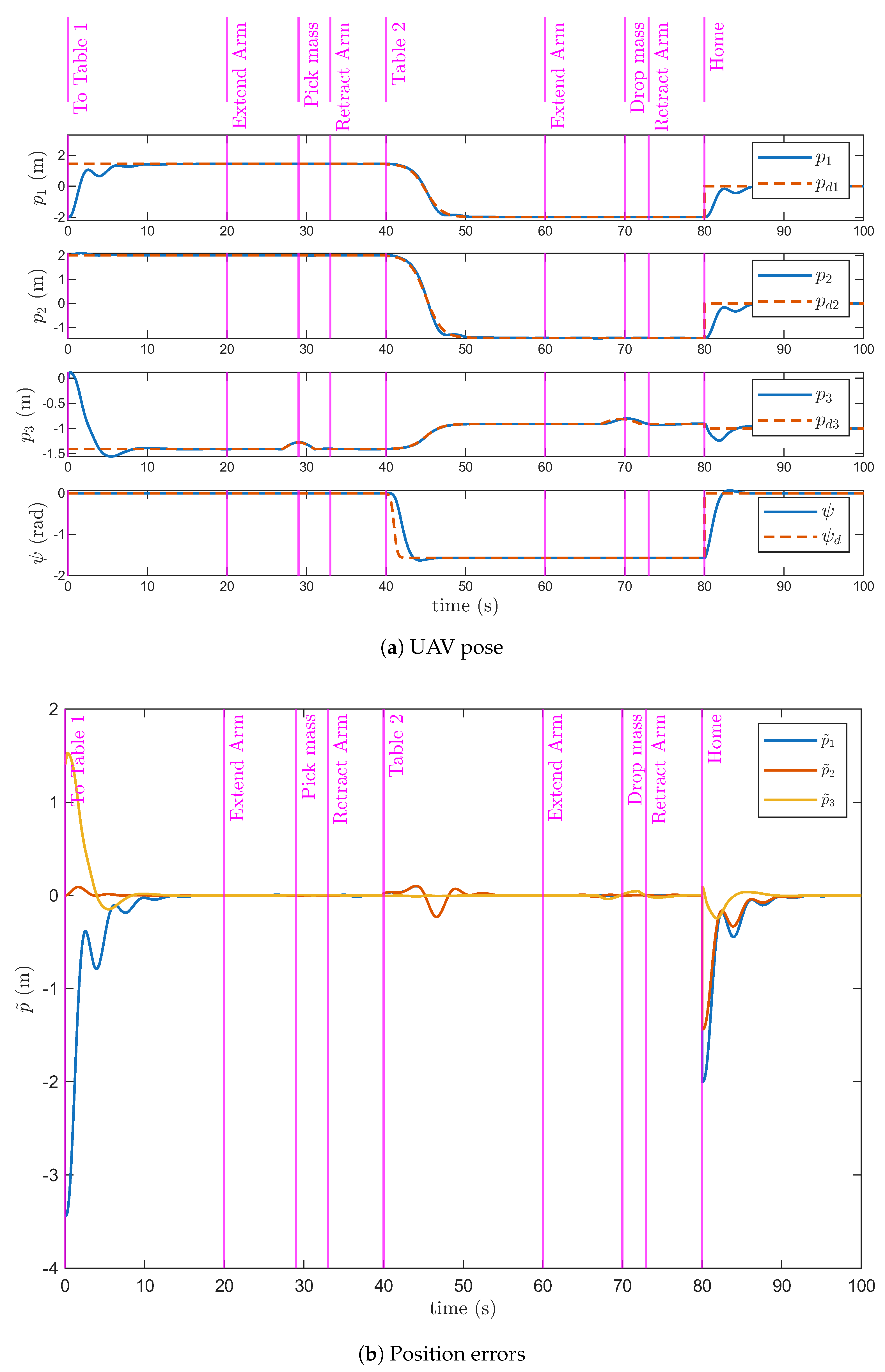
Table 3.
Control Gains
| Parameter | Value | Parameter | Value |
|---|---|---|---|
| 0.4 | 0.5 | ||
| 0.5 | 7 | ||
| 1 | 3 | ||
| 0.001 | 5 | ||
| 1 |
Table 4.
Object pick and place sequence
| Time t | Desired Position | Desired Yaw | Arm configuration | Cube Location |
|---|---|---|---|---|
| 0 | Home | Table 1 | ||
| 20 | Extending | Table 1 | ||
| 27 | Extended | Table 1 | ||
| 29 | Extended | UAM | ||
| 32 | Retracting | UAM | ||
| 40 | Home | UAM | ||
| 60 | Extending | UAM | ||
| 67 | Extending | UAM | ||
| 70 | Extended | Table 2 | ||
| 73 | Retracting | Table 2 | ||
| 80 | 0 | Home | Table 2 |
Disclaimer/Publisher’s Note: The statements, opinions and data contained in all publications are solely those of the individual author(s) and contributor(s) and not of MDPI and/or the editor(s). MDPI and/or the editor(s) disclaim responsibility for any injury to people or property resulting from any ideas, methods, instructions or products referred to in the content. |
© 2025 by the authors. Licensee MDPI, Basel, Switzerland. This article is an open access article distributed under the terms and conditions of the Creative Commons Attribution (CC BY) license (http://creativecommons.org/licenses/by/4.0/).
Copyright: This open access article is published under a Creative Commons CC BY 4.0 license, which permit the free download, distribution, and reuse, provided that the author and preprint are cited in any reuse.


