Submitted:
26 August 2025
Posted:
27 August 2025
You are already at the latest version
Abstract
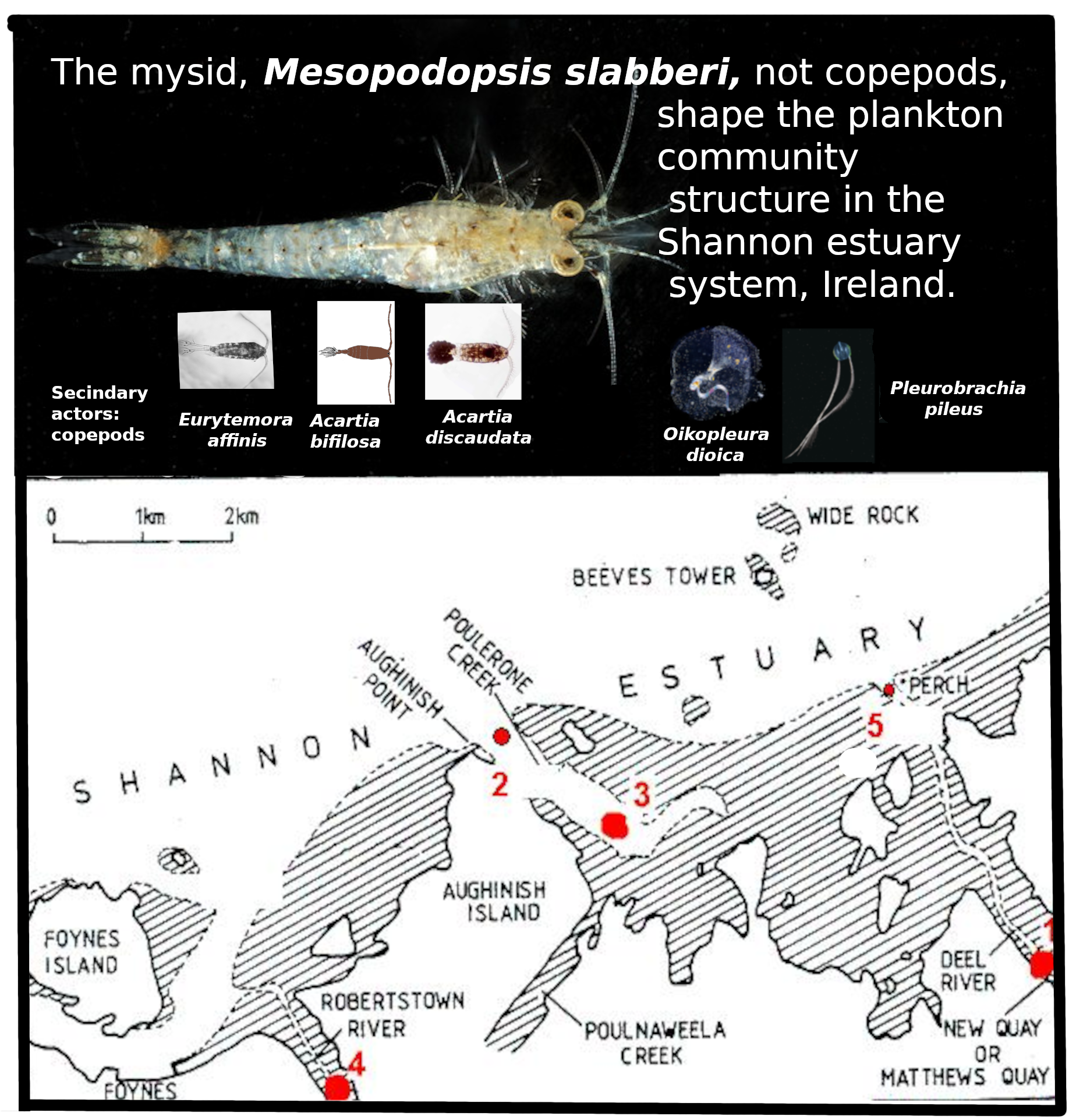
Mesoplankton (netplankton >250 µm) were sampled over one year at three stations in the Shannon Estuary system, Ireland. A net with three mesh sizes was used to capture a wider range of plankton sizes than a standard single-mesh net. An innovation was the incorporation factorial analysis of celestial (seasonal) variables, spring equinox (Spr) and summer solstice (Sum), together with physicochemical and biological variables, without presuming cause or effect. Principal Component Analysis extracted dimensions D1, D2, and D3 accounting for 26%, 17%, and 12% of the variance, respectively. In the D1-D3 plane, Spr and Sum were positioned ~90° apart. Theapproximate trophic impact of by major taxa was estimated from abundance and published clearance rates. Overall, the mean herbivorous/detritivorous clearance by mesoplankton was 54 L·m⁻³·d⁻¹. Of this, mysids, Mesopodopsis slabberi (predominantly April–November), contributed 96.3% and the appendicularian Oikopleura dioica (May–October) 2.0% (nano- and pico-plankton) and copepods only 0.98%. The ctenophore Pleurobrachia pileus (present April–October) cleared an 2.0% (carnivorous clearance). Mysids and copepods contributed additional unquantified carnivorous clearance. These data, collected 45 years ago, provide a valuable baseline for assessing subsequent ecological changes.
Keywords:
mesoplankton
; zooplankton
; estuary
; ireland
; trophic impact
; community structure
; mysids
; copepods
; ctenophores
; appendicularians
1. Introduction
Temperate estuaries are being degraded rapidly worldwide [1]. The Shannon estuary complex, however, is still relatively unpolluted [2,3,4,5] and is internationally important not only as a refuge for wildfowl and waders but also for its important, but strongly threatened, migratory eel [6] and salmon [7] fisheries.
The west coast of Ireland is the most westerly coast of northwest Europe (excluding Iceland), and its estuaries are those which mix with highly oceanic Atlantic Ocean water and its plankton. Yet mesoplankton has been little studied in Irish west-coast estuaries. The only year-round study appears to be that by , the Dunkellin estuary at the head of Galway Bay in salinities of 4.5 to 34.5, using a 160-µm mesh net. Some studies of West-of-Ireland coastal mesoplankton, including those in salinities <30, have included decapod adults and their planktonic larvae [9], copepods [10] , larval and post-larval fishes chaetognaths [12,13] , planktonic cnidaria [14] . The account by [15] of netplankton, sampled in the Shannon estuary in salinities of 25 to 35 in September1977, May 1978 and August 1978, are mentioned further in the Study Area section.
Old ecological studies like the present one are essential for long-term assessments of change in abundance of zooplankton and some fishes [17], particularly with respect to understanding the effects of cyclic and progressive climate variations.
Before the present study began, construction had started on Aughinish Island in the Shannon estuary (Figure 1) of the largest plant in Europe purifying bauxite to alumina (aluminium oxide). Production started in 1983, with a throughput of 800,000 tonnes per year [18]. Concern about the possible ipacts of the plant and its attendant extra shipping promoted fuding of ecological baseline surveys of the plankton and intertidal biota, which were carriedout _from 1978 980 [19,20,21,22]. This paper is based on the netplankton samples (~0.2 to ~2 mm, and larger), sampled during a programme of cruises bauxite purification site on Aughinish Island, on the southern (County Limerick) side of the Shannon estuary, including in two tributary estuaries, the Deel and the Robertstown (1). It complements the accounts by [21,22] of the autotrophic and heterotrophic nano- and micro-plankton (10 µm to 200 µm), sampled during the same cruises.
The aims of this publication are three-fold: 1) to provide an annual record of the netplankton around Aughinish Island in 1979/80 as a basis for assessing chanes during nearly half a century of increased industrial impact in the estuary, climate change and possible species introductions; 2) to use data on plankton abundance to estimate differential grazing pressure (clearance rate) by the major taxa; 3) to present a factorial analysis that relates the mesoplankton community to ceestial, physicochemical and other bioogical (abundance of detritus and pico- and nanoplanktonee. This forial analysiis aims to escape from the presumptive classification of all variables as either controlling or controlled.
This paper is a companion paper to the report on nano- and micro- plalnkton (10 µm) sampled by bottle on the same cruises [22].
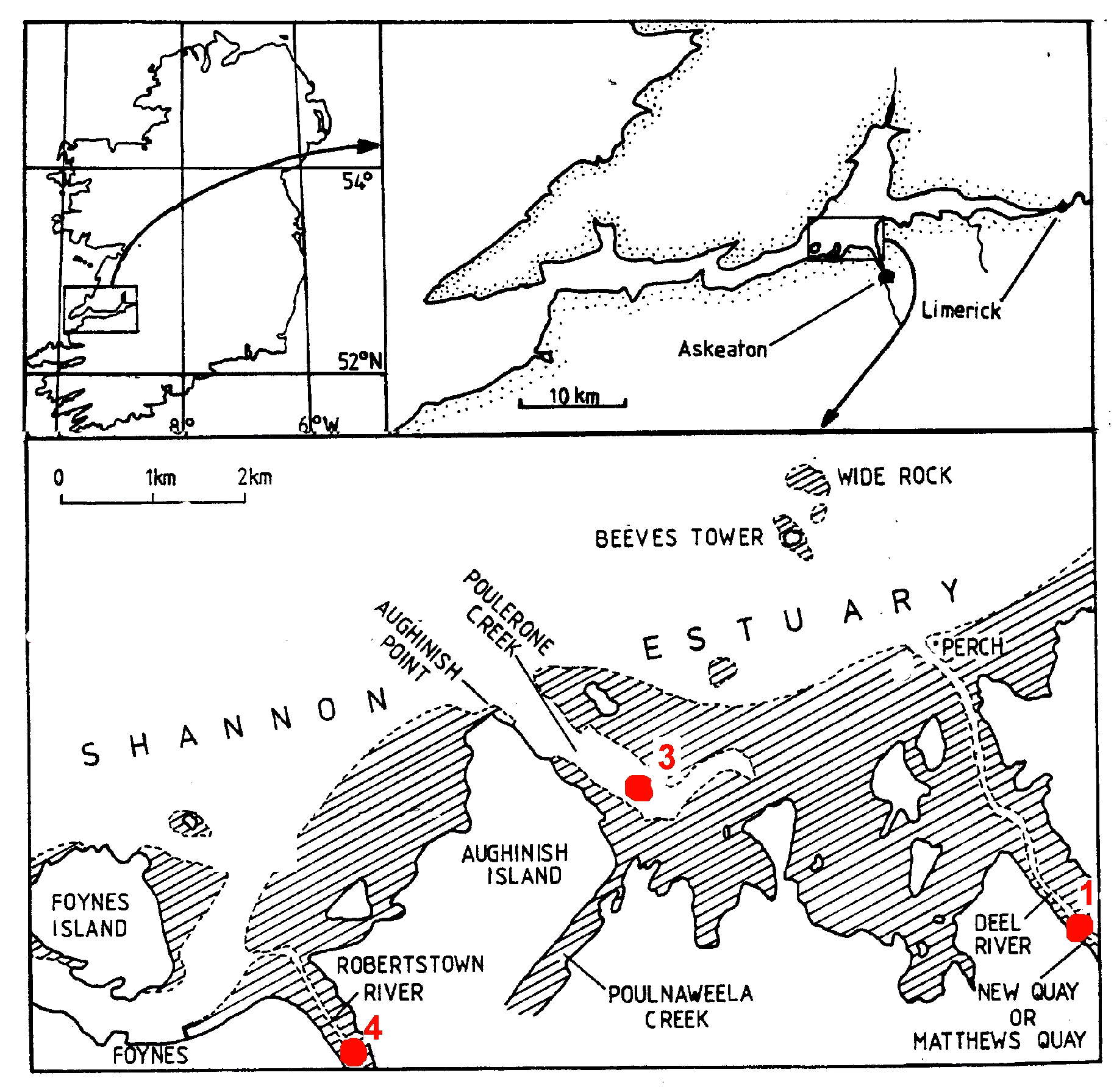
Figure 1.
Upper right – Ireland; Upper right -Shannon estuary; Lower panel – study area. All the five stations marked in red were worked (Jenkinson, 1990), but only stations 1, 3 and 4 were sampled for netplankton. Stations 1 and 4 were sampled by towing against the incoming tide. Station 3 was sampled by towing towards station 3/.
2. Study Area
The River Shannon is considered he longest river in Ireland and Britain, with a length of about 258 km from its source to Limerick City (1), where it meets salt water. It has also by far the greatest annual discharge rate, which at Limerick City is 208 m3.s-1. From there the estuary stretches afurther 101 km to a line from Kerry Head to Loop Head, where it meets the Atlantic Ocean . The river comprises many lakes and drains a catchment area of 11,794 km², mostly agricultural land and peat bog. Into the Shannon estuary, 235 km² in extent, including intertidal areas, flow the rivers Fergus, Owengarney, Deel, Maigue and Robertstown, with their own estuaries, that of the Fergus being extensive, shallow and with many islands and intertidal flats( 1).The Shannon estuary complex is still relatively unpolluted [2] and is internationally important not only as a refuge for wildfowl and wadering birds but also for its salmon runs (Anon. and Conservation through Education,2025) [7] . However, by the 1980s, the estuary was receiving domestic effluent from adjacent towns, notably Limerick, Foynes, Shannon Town and Askeaton [2] . Along its banks and tributaries are Shannon airport, with nearly 2 million passengers in 2023 [23] , and potentially polluting industries at Newmarket-on-Fergus (pharmaceuticals), Askeaton (milk products; plastics) and Tarbert (oil-fired power station), as well as the bauxite plant, as mentione, which has been productig of 1.9 x 10⁶ tonnes y-1 of alumina from bauxite [24] . Additionally, a power station has started at Money Point, burns ~2x10⁶ tonnes coal.y-1. Since the early 1990s shipping traffic has increased to bring this coal and bauxite to the Money Point and Aughinish Island plants, respectively, increasing the likelihood of species introductions [25] .
Measurements of oceanographic parameters, temperature, salinity stratification, turbidity, nutrient and chlorophyll a concentrations, were carried out [26,27] on five cruises from 1977 to 1979. The stations were worked in mid-channel up to Aughinish Island, from which [15] analysed the samples, taken by Clarke-Bumpus nets : for zooplankton, . [28] reported the stratification, nutrients, chlorophyll a and suspended matter concentration and current speeds from Tarbert up to Limerick Town, again mainly in mid-channel. They also modelled the light regime in the water column, and its impact on phytoplankton growth. The chlorophyll a levels they measured showed a strongly negative relationship with salinity. This reflected a combined turbidity and chlorophyll maximum in salinities of 1 to ~6 from 1 to 16 km below Limerick Town, and most of their samples were taken downstream of this turbidity maximum or in it.
This study is based on mesoplankton sampled around Aughinish Island on 9 cruises in 1979 and 1980 [29] . Information on nano- and micro-plankton, obtained during the same cruises has been published [21,22,30]. A related study, on the intertidal and benthic fauna around Aughinish, has also been published [19,20,30], and some of the fauna found in it are common to the plankton we sampled.
3. Materials and Methods
3.1. Sampling, Identification and Estimation of Abundance
Sampling for physicochemical parameters and nano plankton was carried out every four to six weeks at stations 1 to 5 on nine cruises between May 1979 and May 1980. All cruises took place during Spring Tides except for that in August, which was delayed by bad weather and took place during Neaps. Stations were sampled on the rising tide, Stations 1, 3 and 4 being sampled 0h28 to 1 to 2h02, 1h58 to 3h51 and 3h13 to 4h57, respectively, after Low Water Tarbert [22] .
At all sampling stations, observations were made for water clarity (Secchi disc) and temperature/salinity (T/S) vertical profiles, while surface samples were taken for enumeration of microplankton [21,22]. T/S vertical profiles were obtained using an M5 T/S bridge (Electronic Switchgear, Ltd., Chertsey, England). At Stations 1, 3 and 4, a net tow was made, steaming against the incoming tidal current. T/S and other measurements preceded the tow, so the tow may on occasions have taken place in water of salinity somewhat higher by an unknown amount than that recorded.
Figure 2.
Diagrammatic representation of the ring net. Not to scale.
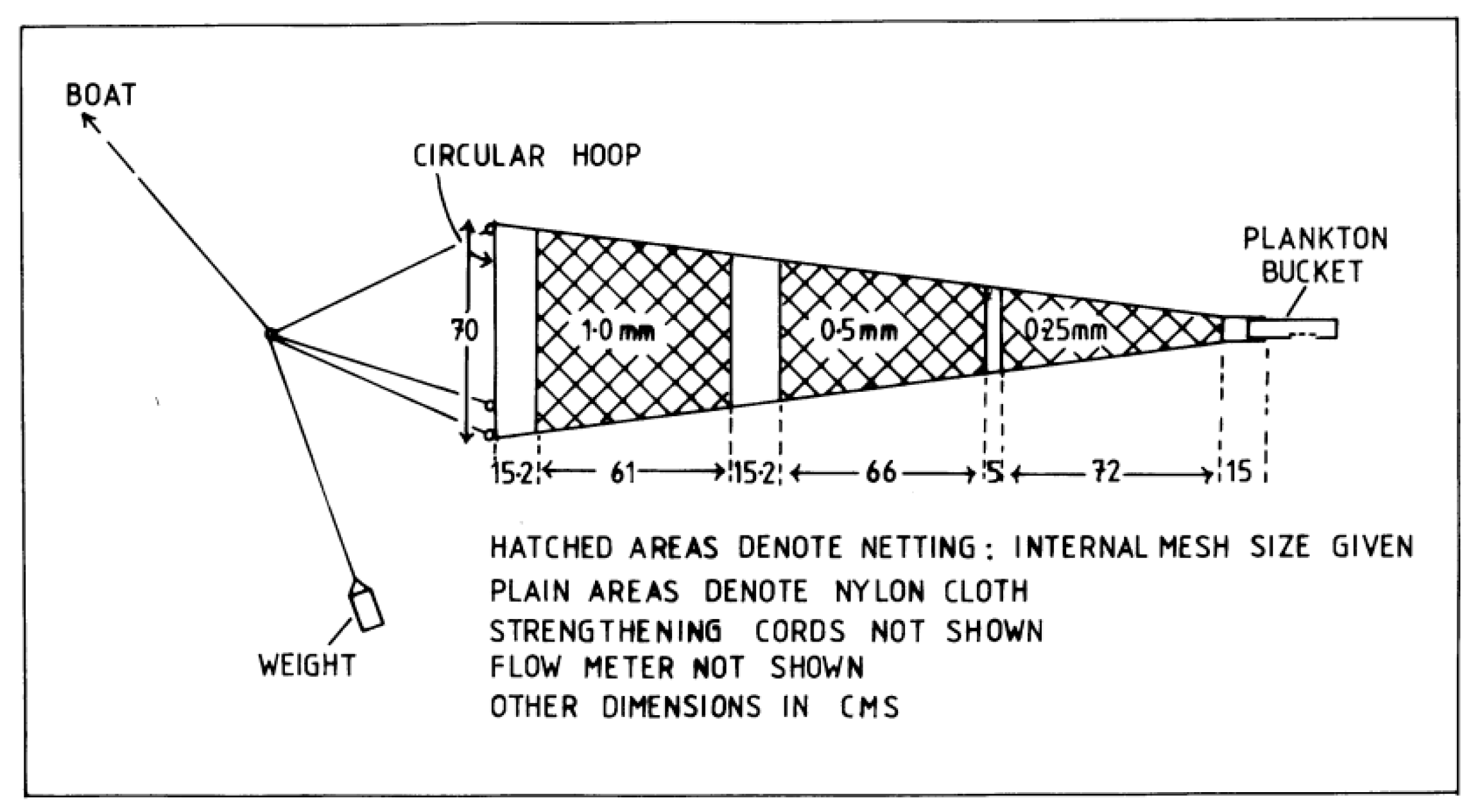
The standard method of sdampling mesoplankton is towing a WP2 net of a single 200-µm mesh [29] . As the present study aimed to obtain information about a wider size range of zooplankton we opted for a net of three mesh sizes 250 µm, 500 µm and 1000 µm ( 2). (Figure 2).
Mesoplankton was sampled by an oblique tow for 10 min at ~1 m.s-1. To estimate the volume, of water filtered by the three mesh sizes the ring of the net was fitted with a flkowmeter fixed a third of the distance across the ring diameter. The net was initially calibrated by towing the ring without a net for a measured time at a measured speed through the water. T The flowmeter reading in real plankton tows then used to estimate the volume of water filtered, and recorded flowmeter reading was then used as a reference against which to estimate the volume filtered by each mesh size. Because filtering efficiency in nets is inversely related to mesh size,we multiplied the estimated volume filtered by the smalles mesh t (200 µm) by a filtering efficiency coefficient of 0.88 [30] although this would have changed as an unknown functionof of clogging by plankton and detritus. The concentration of different-sized organisms was calculated from the estimated volume of the water filtered by each mesh size. The plankton was fixed and preserved in 4% formaldehyde (w/w) in seawater.
The high abundance of comparatively large mysids in our samples prompted us to calculate the estimated clearance rates of the main taxa. Even with the uncertainties in our estimates, it is clear that the the mysid, Mesopodopsis slabberi, played a dominant role in trophic crafting of the zooplankton community structure (see Results section). This study may thus lead to better quantitative understanding of secondary production processes in the planktonic food web 45 years ago, than would have been oossubke had a standard WP2 net been used.
We took the volume sampled (before correction for flowmeter reading) per standard haul to be: 210 m3 for organisms >1.0 mm (Pleurobrachia pileus and other large organisms such as fishes and mysids) sampled by all the three meshes (1.0, 0.5 and 0.25 mm); 100 m3 for organisms >0.5 mm (adult Calanus) sampled by only the smallest two; 37 m3 for plankton >0.25 mm (adult copepods and large copepodites, as well as Oikopleura dioica (without its mucous house) sampled by only the smallest mesh. For detritus, the volume sampled has been taken arbitrarily as 100 m3.
The volume of net-sampled detritus was measured by allowing detritus and plankton to settle together in a measuring cylinder, and the widely varying proportion of each component was estimated by eye.
3.2. Statistical Analyses
3.2.3. Diversity
Community structure was investigated using diversity indices .
Species diversity was calculated from the raw counts using the Shannon-Wiener information function
where pi is the number of individuals of species i in sample s divided by the number of individuals of all species in sample s [31,32,33,34].
Some authors use loge instead of log2 to calculate H', and other authors leave it unclear which method they used. The help files about "diversity" in the "vegan" statistical library [34,35] remark that using log2 or loge makes very little difference. To test this we calculated H' for our data using both methods (data not shown). Values of H' calculated using loge were higher than those calculated using log2, but the difference in all cases was <0.4%.Thus, different studies reporting H' may be compared with less than 1% error.
The Margalef diversity index (also known as "richness"),
where N is the total number of organisms and S is the number of species
Dmg = (S - 1) / (log2 N)
Evenness,
I' = H' / (log2 N)
3.2.3. Principal Component Analysis (PCA)
Community structure was also investigated using and by different factorial methods Only the results of Principal component analysis (PCA) are shown here as they gave the the most intuitively useful results. An innovation is the incorporation of two variables, Spring versus Autumn Equinox (Spr)and Summer versus Winter Solstice (Sum). These may help the reader to follow the role of the annual cycle in 2-D PCA scatter plots (see Rusults section).
3.3. Choice of Environmental Variables
In factorial analysis of environmental time-series data, the distinction between causative and effect variables is difficult. Biological and some physico-chemical data may affect each other over the time scale of the time series, possibly with time lags or feed-back, or both,. We have thus treated all variables similarly. avoiding this distinction. Another innovation in this study is characterizing the annual cycle in terms of progression around a circle that this progression represents the annual cycle as components of spring-autumn equinoxes and summer-winter solstices, which we feel is adapted to subtropical, temperate and boreal zones without a marked monsoon. This includes Ireland. The circle is then defined by these components, Spr and Sum (Equations 4 and 5). To our knowledge this ancient treatment is innovative as an input to ecological time series studies. Longobardi et al. [38], however, used photoperiod, strongly related to Sum, as a variable to investigate phytoplankton abundance and community structure in a Mediterranean study, and found that it had a remarkably stable influence over a time series of 25 years.
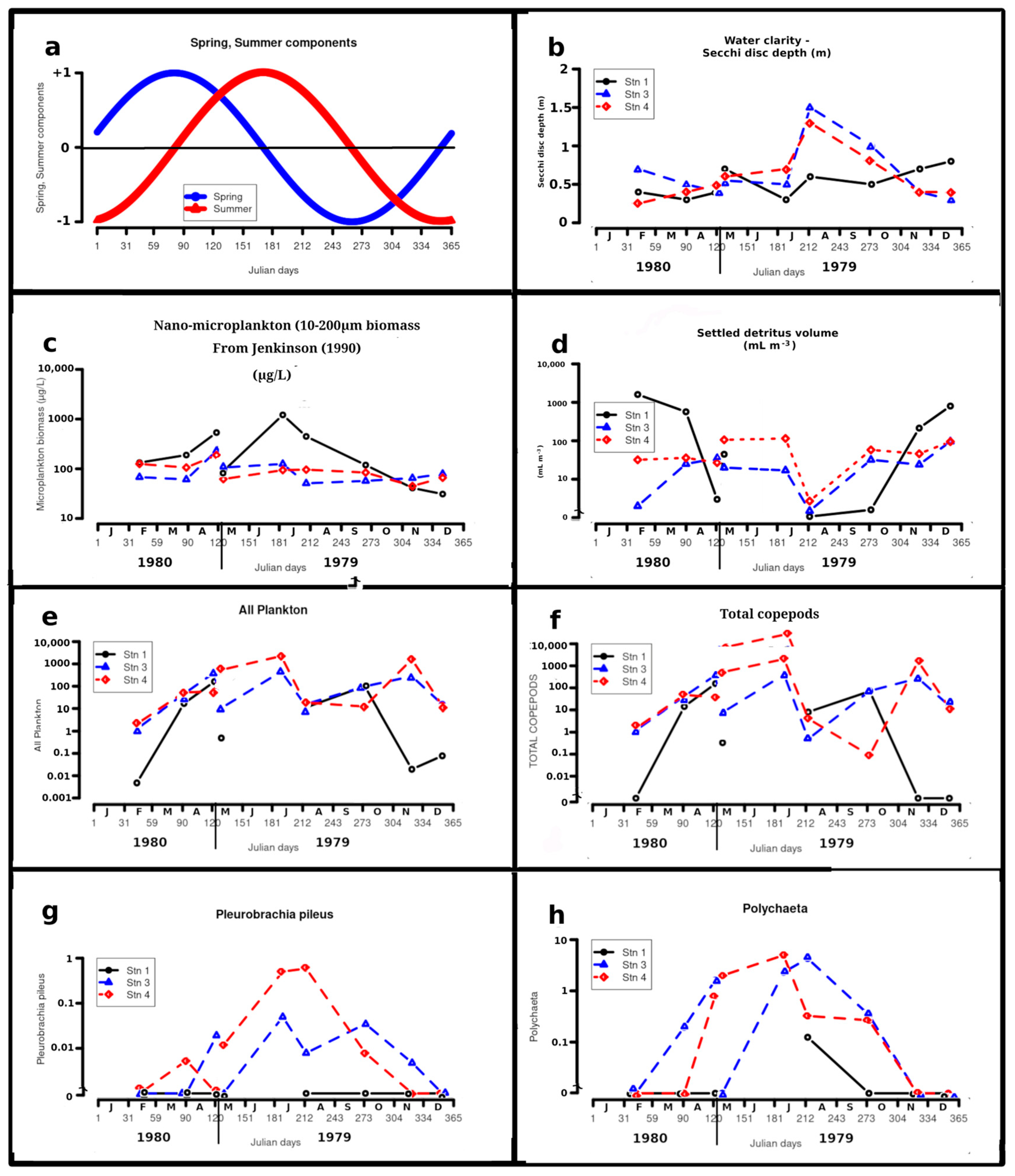
Celestial cycles,, notably the solar annual cycle, produce regular variations in temperature and light flux, particularly in polar and temperate regions, clearly shown in the present annual survey(Figure 5a,c,e). The lunar ~12.64-h M2 cycle is the strongest driver of the tidal cycle in the study area, and aliases with the weaker 12.00-h solar S2 cycle to produce oscillation between spring and neap tides every 14.75 days or so. The solar and lunar cycles have also driven many organisms to develop biological clocks keyed to the annual, lunar-monthly and daily celestial cycles [39] . Other ccycles and environmental fluctuations add furthr variations or “noise”. The present investigation is suitable to detect only annual variations, not lunar or daily variations. We have therefore incorporated into the PCA, the components of Summer solstice, Sum, and Spring equinox, Spr ( 6a). We attempted to minimize interference from lunar-monthly variations by sampling, as closely as possible, always at Spring tides (with the exception of August, which was sampled during Neaps, as mentioned above).
The relationships between environmental and seasonal variables and the most abundant species have been explored using Principal Component Analysis using raw data for physicochemical data and log(n+1) transformation for plankton counts using the "factoextra" package . The spring-autumn equinox component, Spr, and the summer-winter solstice component, Sum, are calculated, as
where Jd is the Julian day. Note that Autumn equinox and Winter solstice components are thus -Spr and -Sum, respectively, and their annual variations are shown in Figure 6a. They may furthermore be imagined them exactly opposite Spr and Sum in the D1-D2 and D1-D3 planes of the PCA analyses (Figure 5a,b).
Spr = +sin(Jd+11)*360/365]
Sum = -cos(Jd+11))*360/365]
3.4. Calculations of Trophic Impact
3.4.1. General Consderations
Trophic impact (as clearance rates) have been estimated for the four principal types of plankton sampled: 1) the ctenophore, Pleurobrachia pileus; 2) copepods (>90% Eurytemora affinis and Acartia spp.); 3) the mysid, Mesopodopsis slabberi; 4) the appendicularian, Oikopleura dioica. Other taxa are considered too minor to have exerted significant trophic pressure. These clearance rates were calculated from abundance and published measurements of clearance (see below). These published measurements generally were not investigated in in relation to different temperatures or other environmental conditions that the animals might encounter, such abundance and composition of food, detritus and predators. Also they were made under laboratory conditions, which may differ from conditions in situ. Our estimates of trophic impact should not therefore be considered too precise. A maximum error of +/- a factor of 5 is thus tentatively suggested.
3.4.2. Predatory Clearance Rate by Pleurobrachia pileus
Båmstedt-[40] measured the clearance rate by P. pileus to be 6.1 L.ind-1.d-1 on the large copepod, Calanus finmarchicus. Pleurobrachia is known to take even larger plankton such as fish larvae [41] , and in the study area,they likely prey considerably on mobile prey such as mysids. It is not clear to what extent the appendicularian, Oikopleura dioica, may be protected from predation by ctenophores such as P. pileus by its mucous house, and its escape reaction when the house is touched by tentacles [42] . In oyr calculations, we have assumed P. pileus carnivorously clears 6 L.ind-1.d-1 for zooplankton and exerts no herbivory or detritivory. We discuss Yap’s suggestion of detrtivory by P. pileus [43] in the Discussion section.
3.4.3. Clearance Rate by Eurytemora affinis
This copepo dfeeds principally on phytoplankton when available, although it can also survive on a diet mainly of detritus, and is thus a widespread and sometimes extremely abundant component of estuarine plankton [44,45,46,47]. In the Shannon, we observed that its gut contained material the yellowish colour of the detritus, confirming its detritivory.
From feeding experiments carried out using natural phytoplankton, Poulet (1978)[48] found that the ingestion rate, expressed as µg.ind-1.h-1 (wet weight),
where POM] is the concentration of particulate organic matter (wet weight g.m-3).
DE = 0.218 + 0.135.POM]
In this case the clearance rate by Eurytemora,
If we assume the existence of a hypothetical phytoplankton population consisting entirely of spheres of diameter 30 µm, and conforming to the relationship between cell volume and content of organic carbon determined by [49] , then 1 g.m-3 (wet weight) equals 52 mg.m-3 of organic C.
Available data [26,27,28]indicate a mean year-round concentation of particulate carbon (POC) level in the Shannon estuary (stations 3 and 4) of ~600 mg C.m-3, of which microplankton contributes ~100 mg C.m-3, except in May when microplankton contributes ~150-200 mg C.m-3 [21,22]. We excluded station 1 from this calculation as its microplankton regime was extremely different from that at stations 3 and 4, with blooms of euglenoids dinoflagellates from May to August ( 6c). E. affinis tends to concentrate near the bottom, where detritus concentrations are typically higher than the average for the water column, and laboratory observations indicate that they are attracted by sediment, regardless of whether it is settled or in suspension [50] . Because of this behaviour, we will assume a mean POC content available to E. affinis in the Shannon estuary is 1000 mg C.m-3, rather higher than typical measured measured levels, ≥600 mg C.m-3 (≥11.6 g.m-3 wet weight). This concentration of POC would give a clearance rate GE of 3.6 cm3.ind-1.d-1 (Table 3), with POC captured DE equal to 2.9 µg C.ind-1.d-1 (Table 3.
Poulet [48] derived Equation 2 for adult females, and we have assumed that adult males and copepodites have respective clearance rates equal to, and half, that of adult females. Poulet [48] carried out his grazing experiments at temperatures rang ing from 0 to 10°C (compared to ambient water temperature of 6 to 17°C in the present study). Since effects of temperature on clearance rate have apparently not been investigated, we have not attempted to correct for them.
3.4.4. Clearance Rate by Acartia spp.
Adults of all species of Acartia found in the present study are about the same size. All are able to use large proportions of detritus in their diets, but appear to need a certain amount of healthy phytoplankton as well. All Acartia species investigated exhibit “tracking” and can also, unlike, E. affinis, actively grasp larger particles, including small zooplankters [48,51,52,53,54].
Clearance rates for all Acartia in the Shannon estuary have been calculated similarly to those for E. affinis. The experimental data used are those derived by Poulet [48] for adult female Acartia clausi. The clearance rate by Acartia,
where DA is. the ingestion rate by Acartia, expressed as µg.ind-1.h-1 (wet weight)
In the case of Acartia, however, POM concentration cannot be assumed to be equal to the level of POM used for calculating GE,, because of Acartia’s need, mentioned above, for a certain amount of healthy phytoplankton. We will assume that half the detrital POM and all the nano- and microplankton POM contribute to the POM available for Acartia. Except at station 1, the concentration of microplankton POC is fairly constant off Aughinish throughout the year, around 100 mg.m-3 [21,22]. The POC available to Acartia is thus estimated as roughly constant at about 460 mg.m-3, or the equivalent of 8.8 g.m-3 (wet weight) if it were all composed of spherical phytoplankton cells 30 µm in diameter [49] . Substituting 8.8 for POM] in Equation 4 gives a clearance rate by Acartia of 0.125 mL.ind-1.h-1, or 3.0 cm3.ind-1.d-1. Carbon is thus captured at the estimated rate of 1.4 µg.ind-1.d-1.
By comparison, Roman [53] experimentally determined clearance rate in Acartia tonsa to vary between 1.5 and 3.7 mL.ind-1.d-1 when fed detritus particles 10 to 24 µm in size composed of aged Fucus, while Kiåørboe et al. [54] found it to dome at 11 mL.ind-1.d-1, for a food concentration (cultured Rhodomonas) of ~150 µg C.L-1, although the latter situation without detritus seems far from the situation in the Shannon estuary.
We have assumed clearance rates by Acartia of 3.0 and 1.5 mL.ind-1.d-1 for the adults and copepodites respectively. Thus grazing pressure by the Acartia population, expressed as mL.m-3.d-1,
where AA is the concentration of adults (m-3) and CA is that of copepodites.
GA = (AA . 3) + (CA . 1.5) (mL.m-3.d-1)
3.4.5. Clearance Rates by Mysids
The mysid population was overwhelmingly dominated by Mesopodopsis slabberi, to which we confine our attention. Mysids, including M. slabberi, are generally omnivorous, feeding raptorially on zooplankton when this is available, but otherwise filter-feeding on phytoplankton or other suspended or settled organic matter [47,55,56].
While predation on phytoplankton is reduced when zooplankton prey is sufficiently abundant (David et al., [47] , clearance rates appear to have been quantified only for filter feeding in the absence of animal prey. [55] studied ingestion rates of M. slabberi sampled from outside a coastal surf zone (S. Africa), fed high concentrations of the planktonic diatoms, Asterionella glacialis (as A. japonica) (105 to 3×10⁵ cells.L-1) and Anaulas birostris (1.8×10⁴ to 105 cells.L-1). They used incubation times mostly of 3 h, and from the ingestion rates and cell concentrations given in their Figure 1, Figure 2, Figure 3, Figure 4 and Figure 5, clearance rates can be calculated between 8.9 and 33 mL.ind-1.h-1 (0.21 to 0.79 L.ind-1.d-1). Comparative incubations on A. glacialis at 3x10⁵ cells.mL-1 of 13-mm (adult) and 3.5-mm (juvenile) specimens gave respective clearance rates of 0.32 and 0.11 L.ind-1.d-1. Incubations for 12 h carried out at two lower concentrations of A. birostris (0.3×10⁴ and 4×10⁴ cells.mL-1) gave respective clearance rates over the first 2 h equivalent to 0.21 and 0.55 L.ind-1.d-1, although little feeding took place thereafter. Satiation seems an unlikely explanation for this cessation of feeding as it occurred after a similar length of time at both the above concentrations, suggesting that conditions in the incubation may have become unsuitable. Webb et al. [55] found no difference in feeding rate between day and night, indicating that feeding on these small diatoms was by filtration rather than visual. Moreover, David [56] found that feeding,on nanophytoplankton was even more intense at night than during the day.
David et al. [47] estimated grazing by M. slabberi incubated on natural suspended organic matter from the Gironde estuary, France. This environment is more similar to the Shannon estuary than that studied by Webb et al. [55] Grazing and clearance rates were measured by David et al. [47] in 24-h incubations, from measurements of chlorophyll a, which probably represented mainly small particles susceptible to filtration rather than grasping. From their results, clearance rates for adults and juveniles respectively have been calculated at 0.78 and 0.39 L.ind-1.d-1. These are the clearance rates we have used, which are at the upper end of the range found by Webb et al. [55]
3.4.6. Clearance Rates by Oikopleura dioica
King [57] found that Oikopleura dioica reared in mesocosms at 14°C, fed on picobacterioplankton from 1 µm to microphytoplankton of 30 µm, and that it needs a minimum concentration of 40 to 60 mg C.m-3. Without this concentration, at 14°C, it died in a few days, but in excess of it O. dioica doubled in numbers, on average, every day. These O. dioica cleared 200 mL.ind-1.d-1. [58] , working in clear waters in the Gulf of California, measured hourly clearance in situ equivalent to 300 mL.ind-1.d-1, and Acuña and Kiefer [59] found average hourly clearance at 15°C equivalent to only 113 to 25 cm3.ind-1.d-1 decreasing as food concentration (cultured flagellates) was increased from 80 to 1600 mg C.m-3, the latter concentration being perhaps a less natural situation. Taking a rough average, we will assume a clearance rate of 100 mL.larvacean-1.d-1 at temperatures in the Shannon estuary system in summer, when they mostly occurred.
4. Results
4.1. Temperature and Salinity
Figure 3 shows the annual variation for temperatures and salinities. At all stations the highest temperatures were encountered in October (16 to 17°C), while the lowest were found in December (6 to 7°C). There was exceptionally cold weather in January 1980, when ice occurred around station 1 (Cyril Ryan, pers. com.). Station 1 showed thermostratification on all cruises when bottom water could be sampled, with a maximum difference between surface and bottom temperatures of 1.0 deg C in May, and inverse stratification in October of 1.3 deg C, associated with strong salinity stratification. Stations 3 and 4 showed little thermostratification.
Figure 3.
Surface and near-bottom temperature (T)and salinity (S) values. Some near-bottom values are missing because of technical malfunction of the T-S meter.
Figure 3.
Surface and near-bottom temperature (T)and salinity (S) values. Some near-bottom values are missing because of technical malfunction of the T-S meter.
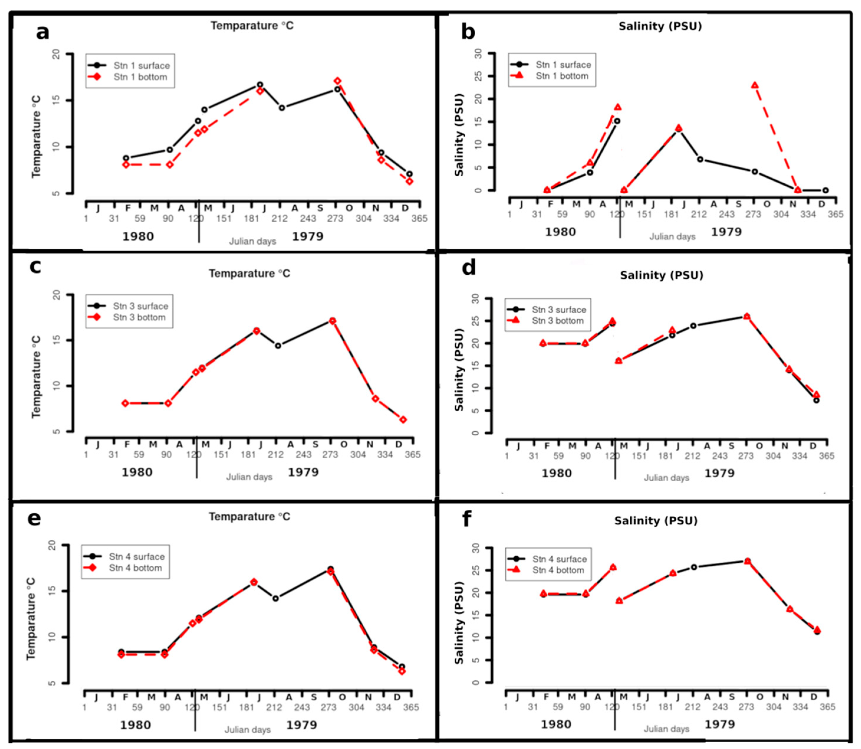
Station 1 was always much less saline than the other stations, with zero salinity in November, December, February and May 1980.. When not occupied entirely by freshwater, it tended to be strongly halostratified. The strongest halostratification here was found in October, with 22.9 PSU in bottom water and only 4.1 in surface water. At stations 3 and 4, the lowest salinities, 7.2 and 9.7 PSU, were found in December and January respectively. At all stations, the highest salinities were found in May 1980 and October,
In summary, station 1 was often strongly stratified when it was not entirely occupied by fresh water. Stations 3 and 4, however, were always well-mixed or only very weakly stratified.
4.2. Etritus Volume Fraction
Figure 6d shows that the volume fraction of detritus ΦD at station 1 varied 23,000-fold, from 7×10⁻⁸ in August to 1.6×10⁻³ in February, and was inversely related to salinity and temperature over the year. At times of high ΦD at station 1, objects such as leaves, small sticks and pieces of wood and paper were sampled. At stations 3 and 4 volumes of detritus varied only by factors of 190 and 67 respectively. At all three stations, detritus was the least abundant on the August cruise, the only one conducted during Neap Tides.
4.3. Total Netplankton
Figure 6e shows that the total numbers of zooplankton at station 1 varied 550-fold, from 0.004 indiv. m-3 in February to 2.2 indiv. m-3 in May 1980. At station 1 netplankton abundance was inversely related to ΦD and positively relatmd to salinity. At station 3, netplankton numbers varied 379-fold, with the minimum, 1.2 indiv. m-3 in February and maxima in July, 455 indiv. m-3, and May 1980, 411 indiv. m-3. At station 4, netplankton numbers varied over 1000-fold from a minimum of 2.1 indiv. m-3 in February to maxima of 2250 and 1613 in July and November respectively.
4.4. Plankton Diversity
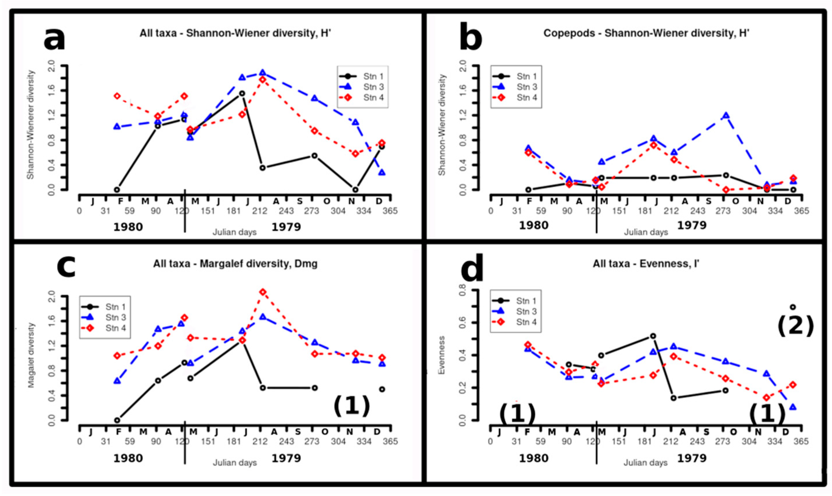
Figure 4a shows Shannon-Wiener diversity, H', values for all taxa. At stations 3 and 4, values were already moderately high (1.0 to 1.6) in February, peaked in August (~1.8) then declined steeply to minimum values in November (0.6 to 1.1) and particularly December (0.3 to 0.7). ( 4b shows H' values just for copepods; at stations 3 and 4, moderate values in February (~1.0) declined to May in both years (0.05 to 0.5), peaked in July for both stations (~0.8), increasing further in October for station 3 (~1.2), then declining to low values in November and December(0.05 to 0.25). 4c shows Margalef diversity (richness), Dmg for all taxa; at stations 3 and 4; fairly low values (0.6 to 1.05) in February increased to peaks in May 1980 (~1.6) and August (1.6 to 2.0), then declined only gradually to December (~1.0). 4d shows evenness, I', At stations 3 and 4, maximum values in February (~0.45) dipped to a minimum (0.2 to 0.35) in May of both years, increased to a second maximum 0.4 to 0.45) in August, then declined gradually to minima in November and December (0.1 to 0.3).
Figure 4.
Netplankton diversity. A – Shannon-Wiener diversity (H’) for all taxa;; b – H’ for copepod taxa only; c – Margalef diversity (also called richness) (Dmg) for all taxa; d – Evenness (I’) for all taxa. Notes (1) – values could not be calculated at station 1 as only one taxon was sampled; (2) – Very high I’ value at station 1 may be misleading as only two taxa were sampled.
For all the four variables, values at station 1 varied widely, and may have been distorted by the low numbers of taxa or individuals, or both, in some samples.
4.5. Principal Component Analysis and Seasonal Distribution
Figure 5 shows the principal component analysis (PCA) of celestial, physico-chemical and biological variables plotted in the hyper space of the the three dominant dimensions (D's), representing 54.1% of the total variance..
Figure 5.
Results of the Principal Component Analysis (PCA), carried out “by station”, with corresponding scores of environmental variables shown on the same plots. a – the D1-D2 plane; b – the D1-D3 plane. Abbreviations for environmental variables are given in Table 1.
Figure 5.
Results of the Principal Component Analysis (PCA), carried out “by station”, with corresponding scores of environmental variables shown on the same plots. a – the D1-D2 plane; b – the D1-D3 plane. Abbreviations for environmental variables are given in Table 1.
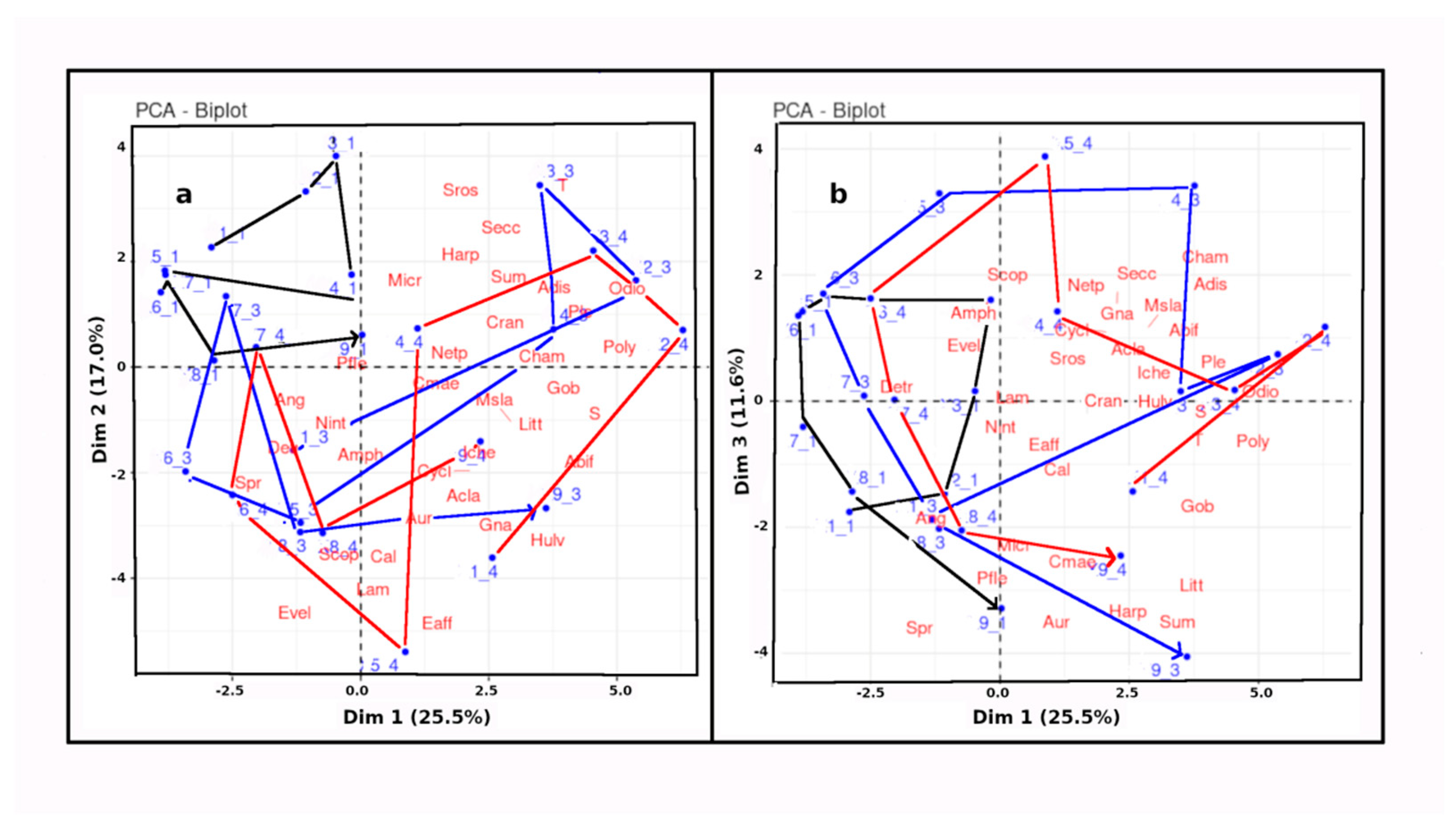

Table 1.
Abbreviaitons of variable shown in Figure 6, and their transformation, if any.
Table 1.
Abbreviaitons of variable shown in Figure 6, and their transformation, if any.
| Abbreviation | Variable | Transform | Abbreviation | Variable | Transform |
|---|---|---|---|---|---|
| Abif | Acartia bifilosa | Log(n+1) | Acla | Acartia clausi | Log(n+1) |
| Adis | Acartia discaudata | Log(n+1) | Amph | Amphipods | Log(n+1) |
| Ang | Anguilla anguilla – elvers | Log(n+1) | Aur | Aurelia aurita | Log(n+1) |
| Cal | Calanus helgolandicus and C. sp. | Log(n+1) | Cham | Centropages hamatus | Log(n+1) |
| Cmae | Carcinus maenas larvae | Log(n+1) | Cran | Crangon crangon | Log(n+1) |
| Cycl | Freshwater cyclopoid copepods | Log(n+1) | Detr | Detritus volume | LoLog(volume) |
| Eaff | Eurytemora affinis | Log(n+1) | Evel | Eurytemora velox | Log(n+1) |
| Gna | Gnathiid isopods | Log(n+1) | Gob | Gobiid larvae | Log(n+1) |
| Harp | Harpactacoid copepods | Log(n+1) | Hulv | Hydrobia ulvae adults | Log(n+1) |
| Iche | Idotea chelipes | Log(n+1) | Lam | Lamellibranch larvae | Log(n+1) |
| Litt | Littorina littorea egg capsules (2-3 eggs) | Log(n+1) | Micr | Biovolume of nano-microplankton 10-200µm (from Jenkinson, 1990)) | Log(volume) |
| Msla | Mesopodopsis slabberi | Log(n+1) | Netp | Total netplankton doncentration | Log(n+1) |
| Nint | Neomysis integer | Log(n+1) | Odio | Oikopleura dioica | Log(n+1) |
| Pfle | Platychthys flesus | Log(n+1) | Ple | Pleurobrachia pileu | Log(n+1) |
| Poly | sPolychaete larvae | Log(n+1) | S | Salinity (mean of surface and bottom) | No transform |
| Scop | Small copepods, Paracalanus parvus and Pseudocalanus elongatus | Log(n+1) | Secc | Secchi disc depth (m) - Water clarity | No transform |
| Spr | Spring equinox component (Autumn component is the negative of this) | No transform | ros | Sygnathus rostratus | Log(n+1) |
| Sum | Summer solstice component (Winter component is the negative of this) | No transform | T | Water temperature (mean of surface and bottom) | No transform |
D1 (variance contribution 25.5%) shows strong positive scores for both temperature (T) and salinity (S), which are generally strongly positively correlated in annual cycles of estuaries in the non-monsoon temperate climates such as those of Europe and North America.
5a shows the D1-D2 plane, D1 and D2 contributing 26 and17% of the variance, respectively. All the samples at station 1 (Deel River) , as well as stations 7_3 and 7_4 (Polerone Creek and Robertstown River in February) are in the top left quadrant, or on its border. Correspondingly, salinity (S) scores in the opposite (bottom right) quadrant. The upper left quadrant is almost devoid of taxa, reflecting low salinity and the low abundance of most netplankton species at ation 1 on all cruises and at stations 3 and 4 in February.
Figure 5b shows the D1-D3 plane. Although D3 contributes only 11,7% of total variance, it adds much intuitive understanding. In the D1-D3 plane, spring equinox (Spr) and summer solstice (Sum) score highly in the bottom left and bottom right quadrants, respectively, roughly 90° aprt. Thus the top right and top left quadrants typify values around the autumn equinox and the winter solstice , respectively. All the stations show anticlockwise rotation over the year. Furthermore, station 1 remains confined to the upper left quadrant in the D1-D3 plane.
Most biological variables scored positively in D1 (summer solstice/autumn equinox and high T and S). Notable exceptions were nektonic elvers of Anguilla anguilla (Ang) and Eurytemora velox (Evel), as well as the physicobiological variable, detritus (Detr). In D2 and D3, Detr scored in opposition to the Secchi transparency (Secc). t
In summary, on the D1-D2 plane, the Deel estuary (station 1) evolved over the year separately from the Shannon (station 3) and the Robertstown (station 4) estuaries, while in the D1-D3 plane Spr and Sum distributed approximately at right angles to each other, with the stations revolving roughly circularly in this plane, following the seasons of the year.
Figure 6.
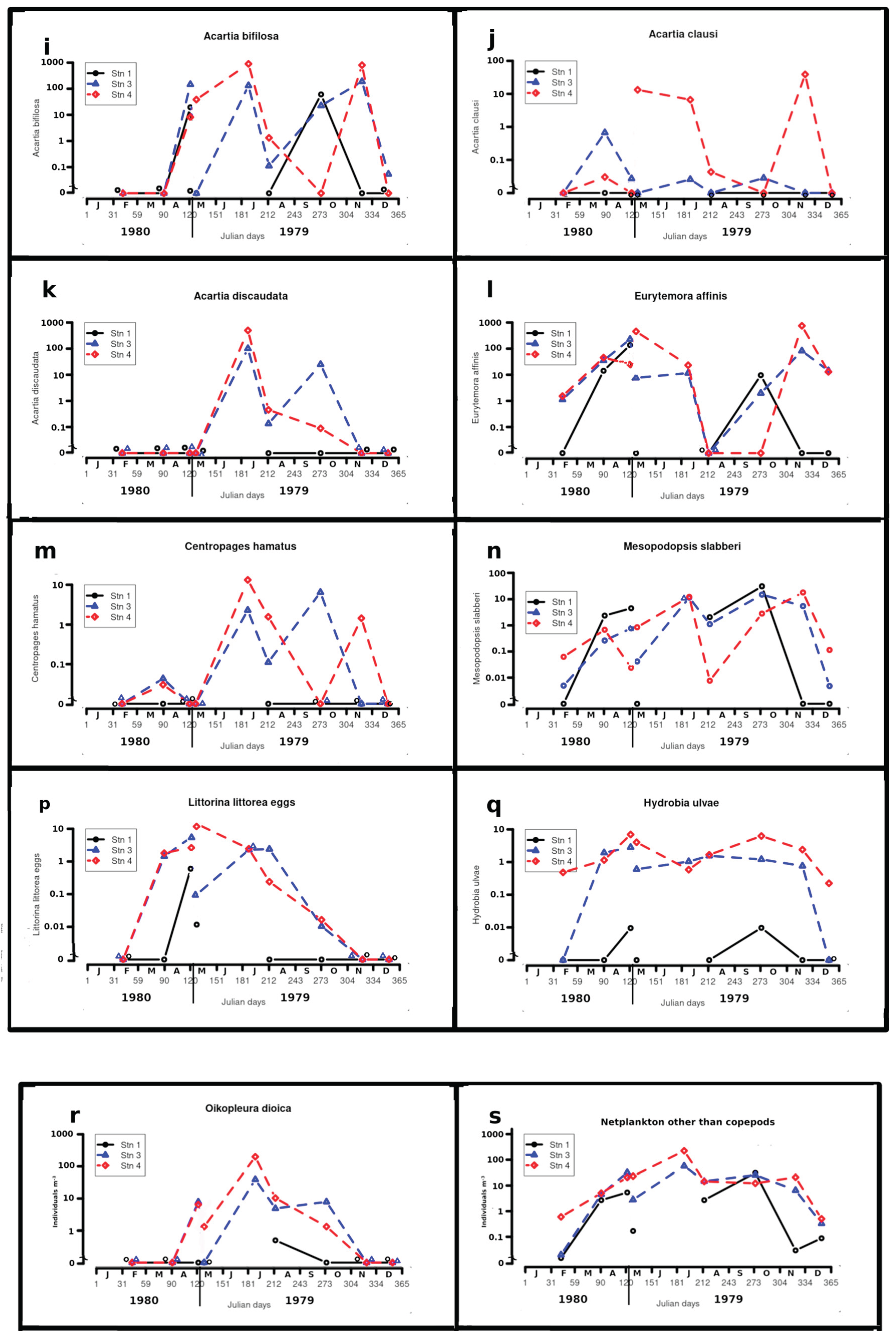
a to s - Annual variations of celestial, physicochemical variables and abundance for the more abundant taxa. Abundance values are omitted for station 1 in July as the sample contained bottom material and was considered non-quantitative.
Figure 6.
a to s - Annual variations of celestial, physicochemical variables and abundance for the more abundant taxa. Abundance values are omitted for station 1 in July as the sample contained bottom material and was considered non-quantitative.
4.6. Dominant and Noteworthy Zooplankton
4.6.1. Coelenterates
Ephyra larva of Aurelia aurita were common in April and May at stations 3 and 4, with a single individual in August, but no medusa-stage was taken. Occasional specimens were taken also of Phialella quadrata, Proboscidactyla stellata, Sarsia gemmifera and Sarsia tubulosa.
4.6.2. Ctenophores
Pleurobrachia pileus (O.F. Müller) ( 6g)
P. pileus occurred from May to October inclusive, at stations with bottom salinities from 16.1 to 27.1. For stations 3 and 4, the mean and maximum concentrations of the species were 0.4 and 4 m-3 respectively, about one third of the values found by Yip [43] over the year in Galway Bay. Yip [43] suggested that P. pileus were ingesting detritus in the Shannon estuary, as their guts contained material of the same yellowish colour and appearance. Another explanation might be that they were predating E. affinis which itself had ingested suspended detritus (see below).
4.6.3. Polychaetes ( 6h)
While specimens were not all identified, the genera Autolytus, lanice and Procena were taken. Tomopteris was not encountered.
4.6.4. Major Copepods (Sex Ratios Are Expressed as M:F. Cited Ratios Expressed as F:M Have Been Converted)
Acartia bifilosa (Giesbrecht) 6i)
With Eurytemora affinis, this was the copepod taken the most abundantly, although it was virtually absent on the cruises from December to April. However, occasional juveniles were taken in November, December and May 1980. It was often abundant at stations 3 and 4, with a maximum of 900 m-3 in July at station 4. It was taken at stations where bottom salinity ranged from 8.5 to 27.0. Overall, the sex ratio was 1:2.9
Acartia clausi Giesbrecht ( 6j)
Taken from May to November. It was sporadically abundant at station 4 (maximum 42 m-3 in November) and occurred at stations where bottom salinity ranged from 16.4 to 27.1. Overall, the sex ratio was 1:9. Its was not taken at station 1.
Acartia discaudata (Giesbrecht) ( 6k)
It was taken at stations 3 and 4, at times abundantly, but only in July, August and October (bottom salinities 22.5 to 27.1), with a maximum of 540 m-3 in July at station 4. The sex ratio was 1:2. It was not taken at station 1.
Eurytemora affinis (Poppe) ( 6l)
It was taken at least at one station on all cruises except in August. With Acartia bifilosa, it was the most abundant copepod sampled, with a maximum (810 m-3) at station 4 in November, in salinities from 5 to 27. Females with eggs occurred from April to December. In November,females with spermatophores were also found. The overall sex ratio was 1:0.65. Bfor comparison, the following sex ratios have been reported. Dutch Wadden Sea: 1:5 [60] ; Gironde: 1:8 to 1:0.45, with positive relationship between the proportion of males and total abundance [50] . In the Seine estuary, Devreker et al., [61] , who made a deailed study of sex ratios, and found mean sex ratio of 1:0,65 in bottom water and 1:0,5 in surace waters.
Eurytemora velox (Lilljeborg)
Taken at station 1 in May 1980 (5 indiv. m-3), when the surface salinity was 15.1. Otherwise occasional specimens were sample at stations 3 and 4, including females with spermatophores in November. The presence of E. velox may have indicated freshwater or brackish salt-marsh run-off.
Temora longicornis (O.F. Müller)
Taken at stations 3 and 4 (2 indiv. m-3) in November (minimum bottom salinity 14.1). Hensey [15] found the species quite abundant in the Shannon estuary, especially in May, but also in August and September. The difference with its distribution in the present survey is unexplained.
Pseudocalanus elongatus Boeck
Taken sporadically at stations 3 and 4 especially in November and April, but also single specimens in May 1979, December and February. Minimum bottom salinity 11.7, and maximum concentration found was 2 m-3 at station 3 in November, where the bottom salinity was 14.1.
According to Hensey t [15] his appears to be a cold-water species in the Irish context, which is consistent with its absence from July to October in the present study. Hensey recorded this species in the Shannon estuary in very great numbers in May 1978.
Centropages hamatus (Lilljeborg) (6m)
It was taken at stations 3 and 4 in April and from July to November. The maximum concentration found was 14 m-3 at station 4 in July. The minimum bottom salinity at stations where it occurred was 16.4. The overall sex ratio was 1:8.7.
In the Shannon Estuary Hensey [15] found the species to be ubiquitous and abundant from Loop Head to Foynes over a salinity range from 25 to 35.
4.6.5. Other Copepods
Isolated specimens were taken of Calanus helgolandicus, Paracalanus parvus, Diaptomus gracilis, Oithona helgolandica, Oithona nana and Caligus curtus. C. curtus is a "sea louse" parasitic primarily on gadoid fishes [62] . Harpacticoids were also taken sporadically on all cruises except in November and December.
4.6.6. Cirripedes
In the present survey, cirrepede larvae were taken at Stations 3 and 4 in May, July and August. In the lower estuary, Hensey [15] found Balanus balanoides larvae abundant in May, and Chthamalus stellatus larvae abundant in August and September.
4.6.7. Mysids
Gastrosaccus spinifer (Goës)
Three specimens at Station 4 in November.
Mesopodopsis slabberi (Van Beneden) ( 6n)
The species was taken on every cruise and at every station except at station 1 from November to February, when salinities were zero. The largest concentrations were 34 indiv. m-3 at station 1 in October, 20 indiv. m-3 at station 4 in November and 16 indiv. m-3 at station 3 in October. In low salinities, adults were often absent or few. Although the presence or absence of eggs was not noted in all samples, adult females with eggs were found in May 1979, July, August, October and May 1980, while non-breeding adult females were noted in May 1979 and August.
This is a euryhaline, estuarine species [63]. Hensey [15] found large numbers of M. slabberi from Tarbert to Foynes, with largest numbers at depths of 10 and 15 m.
Neomysis integer (Leach)
Sporadically, in low to moderate numbers at all stations, on all cruises except October. Most were juvenile, but a breeding female was taken at Station 1 in July.
4.6.8. Isopods
Idotea chelipes was taken on most cruises at Station 4 and occasionally at Station 3. It is characteristically lives among brackish-water intertidal algae.
Gnathiid isopods, most of them apparently Paragnatha formica, were taken sporadically on most cruises. The juveniles, known as pranzias, frequently ectoparasitic on fishes, are often taken in plankton nets [64] .
4.6.9. Amphipods
Sporadic examples were taken including Corophium volutator (Station 4, February) and Metopa alderi (Station 4, July).
4.6.10. Decapods
Carcinus maenas (L.)
Larvae occurred in small numbers in August, and in April and May 1980 (maximum 0.2 indiv. m-3 at stations 3 and 4 in August). The adults were widely distributed on the shore around Aughinish [20] .
Crangon crangon (L.)
These shrimps were taken sporadically in small numbers (maximum ~0.05 indiv. m-3 at station 3 in July). Adults and juveniles were taken in April, May , July (some with eggs), October, November and December (when four adults were taken from zero salinity), April and May 1980. Zoea were taken in May, July and August. Hensey [15] found larvae at all her stations in the Shannon, from Loop Head to Foynes, generally in moderate numbers. Adults were abundant on the shore around Aughinish, especially from May to November [19,20] .
Other decapods.
An adult and a zoea of Micropipus pusillus were taken, as well as a single zoea each of Upogebia deltaura and Anapagurus laevis.
4.6.11. Molluscs
Hydrobia ulvae (Pennant) – adults ( 6q)
They were often abundant, taken at station 4 on all cruises, at station 3 on all cruises except in February and December. At station 1 they were taken only in May and October in very small numbers. Maximum “concentrations” were 12 indiv. m-3 at station 4 in April. O’Sullivan [19] found these snails very abundant on the shores around Aughinish. The adults’ normal habitat is estuarine, or sometimes marine, mud. They generally occur at about mid-tide level, crawling down the beach as the tide ebbs and being floated back up the beach on the flowing tide under the water film [65] or under mucus rafts [66] . That all sampling was carried out during the flood tide may explain the large numbers taken by the plankton net. The small numbers taken in association with low salinities in this survey may be due to the tendency of H. ulvae to remain in their shells when salinities are low [67] .
Littorina littorea (L.) – egg capsules ( 6p)
Egg capsules with two to three eggs were present from April to October. They were the least common at station 1. Maximum “concentrations” were 6 indiv. m-3 at station 4 in May 1979. The adults occur intertidally all around Aughinish [19] , while Hensey [15] found the eggs in the Shannon estuary in September and May. Breeding of L. littorea in the Shannon estuary thus lasts at least from April until late September. Byrne [8] found L. littorea egs in the Dunkellin estuary, Galway Bay. In contrast to our findings, she found them present from January to July.
Other molluscs
Gastropod and lamellibranch larvae were taken sporadically
4.6.12. Tunicates
Oikopleura dioica Fol (6r)
It was present from May to October. It was most abundant at station 4 in July (~200 indiv. m-3) and least at station 1. The minimum bottom salinity at which is was taken was 18.2. Hensey [15] found the species virtually throughout the area sampled in her cruises, in May, August and September. Low salinity appears to limit distribution around Aughinish.
4.6.13. Fishes
The following fishes were taken:
Anguilla anguilla: Elvers (65 to 75 mm) were taken at all stations from December to May, with a maximum of 25 (~0.7 indiv. m-3) at station 1 in April.
Gasterosteus aculeatus: One from Station 1 in November.
Gobiidae: Larval gobies occurred at maxima of ~2 indiv. m-3 from May to November at all stations.
Platychthys flesus: Flounders occurred, the most abundantly at station 1 (~1 indiv. m-3) in April and May. Specimens measured 9 to 10 mm (late larvae and early juveniles).
Sprattus sprattus: Three sprat (yolk-sac stage to 10 mm) were taken atStation 4 in February and May.
Syngnathus rostellatus: Pipefish (16 to 100 mm) were taken mostly singly at Stations 1 and 3, from July to October.
4.7. Clearance Rates and Ingestion Rates
4.7.1. Predatory Clearance Rates by Pleurobrachia pileus
Table 2 shows that the year-round mean clearance rate by P. pileus at Stations 1, 3 and 4 was 0.00, 0.08 and 0.75 L.m-3.d-1 respectively,giving a mean of 0,28 and a maximum clearence rate of 3.5 L.m-3.d-1 at station 4 in August. As clearence by this organism is carnivorous, its clearence rates are not considered together with the herbivorous and herbivorous rates determined for the other major taxa in the study.
Table 2.
Predatory clearance rate (predation pressure) by Pleurobrachia pileus (L.m-3.d-1).
| Station | |||
|---|---|---|---|
| Cruise | 1 | 3 | 4 |
| May | 0.00 | 0.00 | 0.07 |
| Jul | 0.00 | 0.30 | 3.02 |
| Aug | 0.00 | 0.05 | 3.54 |
| Oct | 0.00 | 0.21 | 0.05 |
| Nov | 0.00 | 0.03 | 0.00 |
| Dec | 0.00 | 0.00 | 0.00 |
| Feb | 0.00 | 0.00 | 0.00 |
| Apr | 0.00 | 0.00 | 0.03 |
| May | 0.00 | 0.11 | 0.00 |
| MEAN | 0.00 | 0.078 | 0.75 |
4.7.2. Eurytemora affinis (syn.: Eurytemora hirundoides)
Table 3 shows that year-round mean clearance rate by the E. affinis population at Stations 1, 3 and 4 was 0.05, 0.11 and 0.46 L.m-3.d-1 respectively, the maximum found being 2.9 L.m-3.d-1.at station 4 in November.
Table 3.
Clearance rate by Eurytemora affinis (L.m-3.d-1).
| Station | |||
|---|---|---|---|
| Cruise | 1 | 3 | 4 |
| May | 0 | 0.03 | 0.84 |
| Jul | P | 0.03 | 0.07 |
| Aug | 0 | 0 | 0 |
| Oct | 0.01 | 0.01 | 0 |
| Nov | 0 | 0.29 | 2.9 |
| Dec | 0 | 0.11 | 0.03 |
| Feb | 0 | 0 | 0 |
| Apr | 0.05 | 0.09 | 0.18 |
| May | 0.31 | 0.41 | 0.07 |
| MEAN | 0.05 | 0.11 | 0.45 |
Note - P – E.affnis present but not quatified. Mean excludes Station 1 in July.
4.7.3. Clearance Rates by Acartia spp.
Table 4 shows that mean clearance rate by all Acartia spp. at Stations 1, 3 and 4 was 0.03, 0.24 and 0.67 L.m-3.d-1 respectively, with a mean value of 0.31 and a maximum of 5.5 L.m-3.d-1 in July at station 4. This clearance is applicable to microphytoplankton and detritus caught by filter-feeding. Acartia also catch larger prey such as nauplii by grasping when these are available, but there is still insufficient published information to quantify the trophic impact of this carnivorous feeding.
Table 4.
Clearance rate by Acartia spp. (L.m-3.d-1).
| Station | |||
|---|---|---|---|
| Cruise | 1 | 3 | 4 |
| May | 0 | 0 | 0.08 |
| Jul | 0 | 1 | 5.5 |
| Aug | 0.01 | 0 | 0.01 |
| Oct | 0.2 | 0.17 | 0 |
| Nov | 0 | 0.62 | 0.38 |
| Dec | 0 | 0 | 0 |
| Feb | 0 | 0 | 0 |
| Apr | 0 | 0 | 0 |
| May | 0.06 | 0.38 | 0.02 |
| MEAN | 0.03 | 0.24 | 0.67 |
4.7.4. Clearance Rates by All Copepods
The summed clearance by all copepods (Table 5) (excluding small copepods, copepodites and nauplii, which mostly passed through the net) for Stations 1, 3 and 4 was 0.08, 0.35 and 1.1 L.m-3.d-1 respectively, with a mean of 0.51 m-3.d-1, the maxima found being 5.6 L.m-3.d-1 at station 4 in July and 3.3 L.m-3.d-1 in November.
Table 5.
Clearance rate by all copepods (except small copepodites and nauplii) (L.m-3.d-1).
| Station | |||
|---|---|---|---|
| Cruise | 1 | 3 | 4 |
| May | 0 | 0.03 | 0.92 |
| Jul | P | 1.03 | 5.57 |
| Aug | 0.01 | 0 | 0.01 |
| Oct | 0.21 | 0.18 | 0 |
| Nov | 0 | 0.91 | 3.28 |
| Dec | 0 | 0.11 | 0.03 |
| Feb | 0 | 0 | 0 |
| Apr | 0.05 | 0.09 | 0.18 |
| May | 0.37 | 0.79 | 0.09 |
| MEAN | 0.08 | 0.35 | 1.12 |
4.7.5. Clearance Rates by Mysids
Table 6 shows that Mesopodopsis slabberi (adults and juveniles combined) at Stations 1, 3 and 4 cleared year-round means of 77, 41, 36,73 and 46 L.m-3.d-1 respectively, the maximum found being 491 L.m-3.d-1 at station 1 in October. Maxima at all stations occurred in October or November, with secondary maxima at stations 3 and 4 in July. For each station, the relative contribution by juveniles to total clearance by M. slabberi was only 16% at station 1, but 92% and 73% respectively at stations 3 and 4.
The overall clearance rate, and hence trophic impact, of mysids thus exceeded by about one order of magnitude that of O. dioica, and by about two orders of magnitude that by all the copepods combined. Although the copepods showed the least clearance impact at station 1 (Deel estuary), this was where M. slabberi showed the greatest impact.
Like for Acartia, the present data apply only to clearance by filter-feeding of microplankton, but Mesopodopsis also feeds carnivorously by grasping, particularly on copepod-sized organisms, but no quantitative data appear to have been published for clearance rate due to grasping feeding. The possible avoidance of the net [68] , makes quantitative assessment of mysid abundance difficult, and our estimates of clearance, particularly by adult mysids, could thus have been underestimated.
Table 6.
Clearance rate by Mesopodopsis slabberi (L.m-3.d-1).
| Station | |||
|---|---|---|---|
| Cruise | 1 | 3 | 4 |
| May total | 0.00 | 0.95 | 15.13 |
| Adults | 0.00 | 0.95 | 14.42 |
| Juveniles | 0.00 | 0.00 | 0.71 |
| Jul total | P | 111.84 | 148.25 |
| Adults | P | 7.63 | 66.34 |
| Juveniles | P | 104.22 | 81.90 |
| Aug total | 19.82 | 10.48 | 0.07 |
| Adults | 0.98 | 0.15 | 0.00 |
| Juveniles | 18.84 | 10.34 | 0.07 |
| Oct total | 491.29 | 140.87 | 26.36 |
| Adults | 404.57 | 0.74 | 0.00 |
| Juveniles | 86.72 | 140.12 | 26.36 |
| Nov | 0.00 | 50.93 | 169.38 |
| Adults | 0.00 | 0.00 | 0.00 |
| Juveniles | 0.00 | 50.93 | 169.38 |
| Dec | 0.00 | 0.04 | 1.07 |
| Adults | 0.00 | 0.00 | 0.00 |
| Juveniles | 0.00 | 0.04 | 1.07 |
| Feb | 0.00 | 0.05 | 0.59 |
| Adults | 0.00 | 0.00 | 0.00 |
| Juveniles | 0.00 | 0.05 | 0.59 |
| Apr | 26.26 | 2.56 | 6.34 |
| Adults | 8.36 | 0.21 | 0.00 |
| Juveniles | 17.90 | 2.35 | 6.34 |
| May | 82.50 | 12.84 | 0.31 |
| Adults | 80.41 | 11.23 | 0.18 |
| Juveniles | 2.09 | 1.60 | 0.13 |
| MEAN | 77.48 | 36.73 | 40.83 |
| Adults | 61.79 | 2.32 | 8.99 |
| Juveniles | 15.69 | 34.41 | 31.84 |
| P - Present but not quantified. | |||
4.7.6. Clearance Rates by Oikopleura dioica
Table 7 shows that O. dioica at stations 1, 3 and 4 cleared a mean of 0.014, 0.56 and 2.7 L.m-3.d-1 respectively,giving an overall year-round mean of 1.1 and a maximum of 22 L.m-3.d-1 at station 4 in July. Maxima occurred in July or August at all stations, and the species was found present only from May to August.
Table 7.
Clearance rate by Oikopleura dioica (L.m-3.d-1).
| Station | |||
|---|---|---|---|
| 1 | 3 | 4 | |
| Cruise | |||
| May | 0 | 0 | 0.12 |
| Jul | P | 4.3 | 22 |
| Aug | 0.11 | 0.55 | 1.1 |
| Oct | 0 | 0 | 0 |
| Nov | 0 | 0 | 0 |
| Dec | 0 | 0 | 0 |
| Feb | 0 | 0 | 0 |
| Apr | 0 | 0 | 0 |
| May | 0 | 0.21 | 0.80 |
| MEAN | 0.01 | 0.56 | 2.7 |
P - Present but not enumerated.
4.7.7. Total Filter-Feedingclearance Rates by the Netplankton
Compared with the contribution by copepods, mysids and Oikopleura, the biomass of other herbivores (polychaetes, crustacean and mollusc larvae) appeared negligible. We have thus estimated filter-feeding clearance rates by all the netplankton to be that due to copepods, mysids and Oikopleura.
Estimates of this filter-feeding, herbivorous grazing pressure are presented in Table 9. Dominated by M. slabberi, the herbivorous grazing pressure showed two strong peaks, in May-July and October-November, and two strong minima, in August and December-February. Mean herbivorous clearance rate over the year were 78, 40 and 46 L.m-3.d-1 at stations 1, 3 and 4, respectively , with the overall mean of 54, and a maximum of 491 L.m-3.d-1 at station 1 in October.
4.8. Diversity
The annual variation in Shannon-Wiener diversity, H’, and Margalef diversity , Dmg (also known as "richness"), is shown for all taxa in Figure 4a and Figure 4c respectively. The seasonal variations for each station showed similar, pronounced patterns, but values at station 1 were generally much less diverse than stations 3 and 4. Values for H' showed only moderate seasonal variation at stations 3 and 4, with maxima in August and minima in November and December. At stations 3 and 4, Dmg also showed maxima in August and minima in February as well as in November and December. At station 1, both H' and Dmg showed maxima in July and marked minima in February.
5. Discussion
5.1. Our Three-Mesh Net Was Important to Capture the Larger Amesoplankton
Our three-mesh net sampled a wider size range of plankton than would have been possible using a net of a single mesh, such as a WP2 [29,69].. While some loss of precision must have occurred in our estimates of abundance of the smaller netplankton, the largest mesh (1.0 mm), must have allowed capture of the nekto-planktonic organisms such as mysids and some juvenile fishes. Even so, mysids, which are very active swimmers, may have been undersampled.
An innovation was the inclusion of the astronomical variables Spr and Sum, the trigonometric contributions of the Spring equinox and the Summer solstice, in the factorial Principal Components Analysis (PCA). The Autumn equinox and the Winter solstice are the negative values of Spr and Sum , respectively.
5.2. Trophic Structuring by the Mesoozooplankton
Estuaries generally support zooplankton biomasses that are higher than those of adjacent continental shelves. Different estuaries tend to be dominated by copepods, cladocerans or mysids [70] . Although zooplankton sampling by nets involves important quantitative uncertainties, notably due to net clogging, particularly if detritus is abundant, partial loss of small organisms through the meshes, and net avoidance by the more active organisms. The results of our study are subject to these uncertainties, but may give a wider picture of trophic impact, as well as plankton diversity, than a single-mesh would have done.
The ctenophore, Pleurobrachia pileus, is carnivorous and feeds by trailing two tentacles which entrap and immobilize its prey. Pleurobrachia spp. feed on prey such as fish larvae and mesozooplankton, with copepods observed to predominate [71] . Table 2 shows that trophic impact by P. pileus was confined to the period from May to November. Mean annual clearance rates were 0.00, 0.08 and 0.75 L m-3 d-1 at stations 1, 3 and 4 respectively. P. pileus was not observed at station 1.
The copepod component was dominated by four species, Eurytemora affinis ( 6l), Acartia bifilosa ( 6i), Acartia discaudata ( 6k) and Acartia clausi 6j). A. discaudata and A. clausi were never found at station 1. All three Acartia species showed a distinct minimum during November to February, E. affinis, however, remained abundant throughout the winter, but was never recorded from zero salinity, unlike in the Elbe estuary [72] and the American Great Lakes [73]. The year-round mean estimated clearance rates for all copepods combined (except copepodites and nauplii) was 0.08, 0.35 and 1.1 L m-3 d-1 et stations 1, 3 and 4 respectively (Table 5), nearly two orders of magnitude less than that of the mysids.
The mysid, Mesopodopsis slabberi exerted year-round mean estimated clearance rate of 77, 37 and 41 L m-3 d-1 et stations 1, 3 and 4 respectively. The larger mysid, Neomysis integer, appeared much less abundant and its trophic impact has not been estimated. However, it may have escaped capture more than M. slabberi.
The larvacean, Oikopleura dioica secretes a mucous house with filters with which it feeds on nano- and pico- plankton as well as colloidal organic matter [74]. Its clearance rate, while comparable quantitatively to that of copepods in this study, would have been mainly of smaller particles. than those cleared by the mysids and the copepods. This species was observed only from May to October and at much higher abundances at station 4 than at station 3 and hardly at all at station 1, suggests that it may be advected into the estuary from summer plankton in the lower estuary and the adjacent coastal ocean. Its competitors for food are likely to have been hetero- and mixo-trophic micro- and nano-flagellates [21,22,75]
5,3,. The Net-Zooplankton Community
5.3.1. General Considerations
This section discusses the major observed components of the animals sampled. Some of the larger ones, particularly adult mysids and juvenile fishes may be classed as nekton or nektoplankton. For simplicity they are are here all referred to as "mesozooplankton.
5.3.2. The Major Copepods, Eurytemora and Acartia
Eurytemora affinis, has invaded freshwaters from the sea many times during the last 200 years, so different populations must also have invaded estuaries over the same time scale. [45] suggests that E. affinis constitutes a complex of cryptospecies, morphologically conservative but genetically pre-adapted for rapid evolution in salinity preference. This may explain why the ranges of laboratory-determined salinity tolerance are markedly different for E. affinis from different estuaries. During the last century and a half, motorized shipping has complicated spreading of copepods and their resistant diapause eggs in ballast water. The salinity at which E. affinis occurs in greatest abundance varies widely: between zero for populations recently introduced into the American Great Lakes ) [45] , zero in the Elbe [72]; between 0.5 and 10 in the Weser [76]; zero to 1 in the Gironde [47,77], about 16 in the Shannon (present study); below 30 [44,78]between 20 and 25 [79] in the Severn.
Acartia bifilosa is a “companion species” to E. affinis in many European estuaries. The salinity at which it occurs in greatest abundance also varies: from 15 to 22 in the Gironde [50], from 13 to 25 in the Shannon (present study); and from 27 to 33 in the Severn [78] .
Reporting laboratory investigations of E. affinis from the Dutch Wadden Sea, [60] concluded, “that biotic factors (such as food competition, predation, and parasitism) their parentheses] may be instrumental in countering occupation of the marine habitat by E. affinis”. That the widely occurring estuarine plankton species, E. affinis, A. bifilosa, M. slabberi and juvenile Sagitta, are found in more or less restricted, but different, salinity ranges in different estuaries and other coastal waters, suggests that even if salinity controls the distribution in the short term, other factors may control it at longer times scales, perhaps by forcing the evolution of salinity tolerance. One obvious candidate for such a factor is the type of food available. Levels of suspended sediment and detritus are generally (but not always) highest in the uppermost parts of estuaries, and these are often associated with high levels of heterotrophic bacteria and nanoflagellates, more or less aggregated with detritus into larger particles. Other factors may be the concentration of detritus or its ratio to living phytoplankton. For instance, Chervin et al. [80] found that the rate of copepod development in an estuary (the detritivorous E. affinis was absent) was inversely related to detritus concentration, although levels of chlorophyll were roughly the same throughout the estuary. He concluded that high levels of detritus could prevent effective feeding on phytoplankton by clogging filtering mechanisms. This would affect some species more than others.
Although E. affinis can use phytoplankton [81,82], ciliates [83] and detritus [50,84,85], it can live exclusively on estuarine detritus [50] . By contrast, Acartia app. need some healthy phytoplankton as well [48,51,52,53]. Even when phytoplankton is present in the turbid part of an estuary, too high a concentration of sediment or detritus is likely to reduce the efficiency of A. bifilosa’s search for its food, thus favouring E. affinis. A. bifilosa may out-compete Eurytemora for phytoplankton when sediment and detritus are less abundant. Adults of A. bifilosa have feeding appendages coarser than those of E. affinis, and they can also feed carnivorously [50] . In addition to competing with E. affinis for food, A. bifilosa may control the former species by preying on its nauplii, particularly when the species are co-dominant and phytoplankton suitable for A. bifilosa is scarce.
Acartia tonsa has spread from North America to colonise West European estuaries and coastal waters during the twentieth century, where it is now considered dominant in many estuaries and coastal areas from the Gulf of Finland to the Mondego estuary, Portugal, including British coastal waters [86,87]. As it is considered to be spread by ships’ ballast water (Bradford-Greve, 1999) [86], we here confirm its absence in our samples taken in 1979-1980, while its subsequent appearance should not occasion surprise.
5.3.3. Cladocerans
Cladocerans also were absent from our samples.
5.3.4. Mesopodopsis slabberi
[88] report that Mesopodopsis slabberi occurs in salinities from 1.3 to 43. The same authors partially analysed the genome of M. slabberi from seven estuaries in continental western Europe, as well as of M. wooldridgei from South Africa. They showed that genetic differences between populations in different estuaries are strong, which suggests that genetic movement between estuaries has been low. This, Remerie et al. [88] suggest, may be associated with strong position maintenance by this strongly swimming organism, coupled with brooding of the larvae in a brood pouch. Like Eurytemora affinis, M. slabberi may be a complex of look-alike cryptospecies.
5.3.5. Oikopleura Dioica
Oikopleura appeared at stations 3 and 4 between May and July, after the spring microplankton maximum, and its grazing pressure (maximum 43 L.m-3.d-1, Table 7) may have contributed to controlling the nano- and pico-plankton abundance, but at station 1, where blooms of euglenoids and dinoflagellates occurred [21,22].
5.3.6. Pleurobrachia Pileus
In summer, the mesoplankton suffered additional predation by the ambush predator Pleurobrachia of up to 3.5 L.m-3.d-1 (Table 2), although this seems too weak to contribute significantly to the August copepod minimum ( 6f). Mysids, since they are very mobile, may be particularly vulnerable to this ambush predation. Although Pleurobrachia frequently takes larval fish [41] , there appears to be no published data on predation on mysids by ctenophores.
Position maintenance by estuarinemeso plankton
The ability of estuarine planktonic animals to prevent their populations being washed out to sea is a major factor in determining their autochthonous occurrence in different estuaries. The tendency of E. affinis both to associate with detritus [50] , and the in vitro observation that it tends to sink in relatively still water [76] may lead to its relatively greater occurrence near the bottom [15,50,79], and this in turn may help it to remain in estuaries like the Morlaix [89] , and those with high flushing rates.5,3,7,
5.3.7. The Absence of Cladocerans
5.3.8. Hydrobia Ulvae
Small gastropods Hydrobia ulvae are very abundant on the mud flats around Aughinish [19] . They drift in the water by crawling on to the surface film of the water, as the rising tide covers their mud flats [67] . The proximity of the stations in this survey to intertidal areas and the fact that sampling took place on the rising tide and mainly at Springs are thus all factors which may collectively explain the high abundance of H. ulvae in the plankton-net oblique tows . [92] found that floating by H. ulvae showed a strong fortnightly rhythm, with maxima at Spring Tides, and minima at Neaps. However, this rhythm is not confirmed in the Shannon estuary, as no minimum in our catches of H. ulvae occurred in August, when sampling was done at Neap Tides. The relative scarcity of H. ulvae at station 1 and their absence at station 3 from December to February suggests that they may be limited by salinity <~10 PSU. At station 4 (measured salinities 6.1 to 27.4 in the present study), H. ulvae floated all year round.
5.4. Diversity
In temperate, non-monsoonal estuaries, such as the Gironde [50] , Morlaix Bay estuary [93] , taxon diversity H’ has been found generally highest in summer, and lowest in winter. This can be due to two effects, greater intrusion of allochthonous, halophile species in summer, and the greater biological activity due to higher light levels and higher temperature. The annual patterns of copepod diversity at stations 3 and 4 in the present survey resemble those in the Gironde estuary, but we found the variation to be greater in the Shannon ( 4a).
That the annual cycles of H’, calculated from the different (overlapping) plankton assemblages (Figure 4a,b)) followed much the same patterns at stations 3 and 4 indicates that netplankton taxon diversity gives a measure of some real ecological state in the Shannon estuary. At stations 3 and 4 H’ for all organisms, as well as H’ for copepods alone, showed a positive relationship with total netplankton volume (Compare Figure 4a and Figure 6e), being highest in summer and lowest in winter, and both being higher in May 1980 than in May 1979. H’ for copepods only ( 4b) showed a similar annual pattern to that of H’ for all taxa ( 4a). Its seasonal pattern, however, was completely different from that of copepod abundance ( 6f), remaining high through a 1000-fold crash in abundance and a 100-fold recovery at station 3. This indicated that, in the Shannon estuary system, diversity is not functionally related to abundance. The lowest values of copepod diversity at stations 3 and 4 generally corresponded to overwhelming dominance by E. affinis.
Margalef diversity, Dmg, showed similar distributions to H', although the distinction between Station 1 n the one hand and Stations 3 and 4 on the other was more distinct. Evenness I' distributions '( 4d) are difficult to interpret. The high value at Station 1 in December is likely to be an artefact as only two taxa were sampled.
In this study, the lower low diversity values (H', Dmg) of the total netplankton reflects numerical dominance by either Mesopodopsis slabberi or Eurytemora affinis. While high diversity reflects in part the greater ingress of allochthonous species (e.g.. Pseudocalanus elongatus, Acartia clausi, A. discaudata and to some extent Pleurobrachia pileus and Oikopleura dioica) from the ocean or lower estuary, it also reflects the development of a relatively diverse autochthonous meroplankton fauna which overwinters benthically, such as Hydrobia ulvae, decapod larvae and coelenterates, as well as of Acartia bifilosa. Acartia spp. may be considered part of the meroplankton because of their ability to overwinter as benthic eggs [94]
Despite netplankton, and marine species in particular, being more abundant at station 4 than at station 3 ( 6e), netplankton diversity at the two stations was similar (Figure 4a–c). This strongly suggests that plankton diversity was not just a measure of allochthonous intrusion (which was higher at station 4), but reflected more the autochthonous ecological differences within the estuary. Reduced diversity at these stations in winter probably reflects greater environmental harshness at this season.
That netplankton diversity at station 1 was generally lower than at the other stations indicates that the estuarine environment of the Deel is harsher than that of adjacent parts of the Shannon estuary. This may be related to lower and more rapidly changing salinities, as well as washouts during high river discharge. The virtual absence of freshwater indicator species in the Deel estuary, however, suggests that the Deel river must have been poor in plankton, for either natural or anthropogenic reasons. That the annual pattern of variation in diversity at station 1 was found to be quite different from that at stations 3 and 4 (Figure 4a–c), as was its composition in both netplankton and phytoplankton [21,22]again shows that the Deel estuary is environmentally distinct from the adjacent parts of the Shannon estuary.
5.5. Mesopodopsis Controls the Mesoplankton Food Web
M.esopodopsisslabberi juveniles and adults prefer micro- and mesozooplankton prey to phytoplankton [47,55,56] .David [56] found that, in the Gironde, juveniles take 4% vegetable particulate organic matter, 77% microzooplankton and 19% mesozooplankton, while for adults the respective proportions are 0%, 70% and 30%. Such proportions likely depend on the respective abundance of these different trophic pools. If the proportion of these pools consumed by juveniles and adults of Mesopodopsis is similar in the Shannon estuary to that in the Gronde, it would suggest that not only does Mesopodopsis dwarf the trophic impact by copepods, but that it also heavily impacts the copepods themselves, dominating and retaining them in a secondary role as consumers in the trophic web. Because copepods have a more rapid turnover (shorter life span) than mysids, they may be rapidly repackaging nano- and microplankton flagellates, ciliates and diatoms into higher quality food particles exloitable by the mysids. The juvenile mysids likely exploit some flagellates, ciiates and diatome directly as well. The trophic roles of detritus, with its changing composition, needs further detailed study.
6. Conclusions
-
The mesoplankton in the Shannon estuary system near Aughinish Island, and two tributary estuaries, the Robertstown and the Deel, was investigated in 1979-80 in nine cruises over a year.This archive on the mesoplankton is now available for comparison across spatial and temporal scales.
- The year-round mesoplankton distribution in the Robertstown estuary (station 4) was similar to that at the station sampled in the Shannon estuary (station 3), but that in the Deel estuary (station 1) was quite distinct, corresponding to very different annual vaiaions in salinity and microoplankton.
- The PCA, incorporating our two innovations of leaving controlling and controlled variables undefined, and the incorporation of the celestial variables of Spring-Autumn (Spr)and Summer-Winter (Sum), gave distributions of variables and stations in the first three dimensions, D1, D2 and D3, of hyperspace compatible with human intuition. On the D1-D3 plane, the Deel evolved over the year separately from the Shannon and the Robertstown , while in the D1-D3 plane Spr and Sum distributed approximately at right angles to each other, roughly circularly in this plane, along with the seasons of the year.
- The copepod fauna overall was dominated by Eurytemora affinis, Acartia bifilosa and A. discaudata, as well as the somewhat less abundant A. clausi. This fauna is typical of many temperate estuaries, except for the notable absence of two components, cladocerans and the copepod, Acartia tonsa. A. tonsa an invasive copepod, had already widely colonized European estuaries at the time of this survey. Subsequent colonization of the Shannon estuary system is therefore to be expected.
- Trophic impact ‘clearance rate) by the major groups of mesoplankton are estimated as follows. In the Deel (Station 1), the Shannon (Station 3) and the Robertstown (Station 4), respectively: Mesopodopsis slabberi (herbivorous and detritivorous part), 77.48, 36.73, 40.83 L.m-3.d-1 (mean 51.68); all copepods (herbivorous and detritivorous part), 0.072, 0.30, 0,91 L.m-3.d-1 (mean 0.43); Oikopleura dioica (herbivorous on pico/nanoplankton), 0.014, 0.56, 2.7 L.m-3.d-1(mean 1.09). Thus gives a year-round mean herbivorous/detritvorous mean of 53,20 L.m-3.d-1, of which Mesopodopsis, copepods and Oikopleura v contributed 97.14%, 0.81% and 2.04%, respectively. Additionally, Peurobrachia contributed a year-round mean carnivorous trophic impact in the Deel, Shnnon and Robertstown estuaries of 0.00, 0.08 and 0.75 L.m-3.d-1,(mean 0.28 L.m-3.d-1), while Mesopodopsis and copepods added an unknown amount of extra carnivorous impact. Combined carnivorous impact by Mesopodopsis and Pleurobrachia may have been keeping the larval and adult copepod populations low.
Author Contributions
IRJ obtained the funding, carried out the sampling and wrote the manuscript.. IRJ and THR designed the project. THR identified and enumerated the mesoplankton.
Funding
Funded by Aughinish Alumina Ltd through University College Dublin to IRJ and THR. University College Galway provided materials, laboratory and library facilities.
Data Availability Statement
The raw data are available as a spreadsheet, available to JMBA on request.
Acknowledgments
Their support, liaison and permission to publish are gratefully acknowledged. John Bracken, Brenda Healy, Geoffrey O’Sullivan and Brian McK. Bary facilitated this study, and we also thank Geoffrey O’Sullivan and Mary Hensey for sharing their data. John Coyne and Tom Furey provided important technical help and Cyril Ryan of Askeaton was a superb boatman even in apparently impossible conditions. More recently, Sami Souissi encouraged publication of this work. Co-author Tom H. Ryan died tragically in a car accident, and this paper is fondly and respectfully dedicated to his memory.
References
- Lotze, H.K. , Lenihan, H. , Bourque, B., Bradbury, R., Cooke, R., Kay, M., Kidwell, S., Kirby, M., Peterson, C., Jackson, J. Depletion, Degradation, and Recovery Potential of Estuaries and Coastal Seas Science. 2006, 312, 1806–1809. [Google Scholar] [CrossRef]
- Jeffrey, D. , Wilson, J.G., Harris, C., Tomlinson, D. The application of two simple indices to Irish estuary pollution studies. In: Estuarine Management and Quality Assessment, Wilson J., Halcrow W. (Eds), Plenum Press, London, 1985, pp. 147–161.
- Wilson, J. , Brennan, B. Spatial and temporal variation in sediments and their nutrient concentrations in the unpolluted Shannon estuary, Ireland. Archiv für Hydrobiologie.. 1993, 75, 451–486. [Google Scholar]
- Wilson, J. , Brennan, B., Brennan, M. Horizontal and vertical gradients in sediment nutrients on mudflats in the Shannon estuary, Ireland. Netherlands Journal of Aquatic Ecology. 1993, 27, 173–180. [Google Scholar] [CrossRef]
- Wilson, J. , Brennan, M. Nutrient interchange between the sediment and the overlying water on the intertidal mudflats of the Shannon estuary Archiv für Hydrobiologie. 1993, 75, 423–450. [Google Scholar]
- McCarthy, T.K. , Frankiewicz, P. , Cullen, P., Blaszkowski, M., Oâ'Connor, W., Doherty, D. Long-term effects of hydropower installations and associated river regulation on River Shannon eel populations: mitigation and management Hydrobiologia. 2008, 609, 109–124. [Google Scholar] [CrossRef]
- Anon. and Conservation through Education (2025) All gates closed. The life and death of the Atlantic salmon. https://www.youtube.com/watch?v=PcgFo0odp2w Consulted 2 Jan, 2025.
- Byrne, P. Seasonal Composition of Meroplankton in the Dunkellin Estuary, Galway Bay. Biology and Environment: Proceedings of the Royal Irish Academy 1995, 95B, 35–48. Available online: http://www.jstor.org/stable/20504491.
- Ó Céidigh, P. The marine Decapoda of Counties Galway and Clare. Proceedings of the Royal Irish Academy, Section B. 1961, 62, 151–174. [Google Scholar]
- Fives, J.M. Investigations of the plankton of the west coast of Ireland. II. Planktonic Copepoda raken off County Galway and adjacent areas in plankton surveys during the years 1958 to 1963. Proceeedings of the Royal Irish Academy, B. 1968, 67, 233–259. [Google Scholar]
- Fives, J.M. Investigations of the Plankton of the West Coast of Ireland: IV. Larval and Post-Larval Stages of Fishes Taken from the Plankton of the West Coast in Surveys during the Years 1958-1966 Proceedings of the Royal Irish Academy. Section B: Biological, Geological, and Chemical Science. 1970, 70, 15–93. Available online: http://www.jstor.org/stable/20494950.
- Fives, J.M. Investigations of the Plankton of the West Coast of Ireland: V. Chaetognatha Recorded from the Inshore Plankton off Co. Galway Proceedings of the Royal Irish Academy. Section B: Biological, Geological, and Chemical Science. 1971, 71, 119–138. Available online: http://www.jstor.org/stable/20518893.
- O'Brien, F.I. The relationship between temperatur, salinity and Chaetognatha of the Galway Bay area of the west coast of Ireland. Proceedings of the Ryal Iish Academy, B. 1977, 77, 245–252. [Google Scholar]
- Boyd, R.J. , Céidigh, P. Ó., Wilkinson, A. Investigations of the Plankton of the West Coast of Ireland: VI. Pelagic Cnidaria of the Galway Bay Area 1956-72, with a Revision of Previous Records for These Species in Irish Inshore Waters Proceedings of the Royal Irish Academy. Section B: Biological, Geological, and Chemical Science. 1973, 73, 383–403. Available online: http://www.jstor.org/stable/20518927.
- Hensey, M. (1980) Zooplankton and oceanographic conditions in the Shannon Estuary, Ireland. M.Sc. Dissertation, University College Galway, National University of Ireland, Galway, Ireland.
- Mackas, D.L. , Beaugrand, G. Comparisons of zooplankton time series J Mar Syst. 2010, 79, 286–304. [Google Scholar] [CrossRef]
- Currie, R. , Wyatt, T. , O'Brien, D. Determoinistic signals in fish catches, wine harvests and sea-level, and further experiments Int J Climatol. 1993, 13, 665–687. [Google Scholar]
- Beaulieu, S. The Road to a New Bauxite – Mine and Refinery Optimisation. In: TRAVAUX 48, Proceedings of the 37 th Internati Conal ICSOBA Conference andXXV Conference «Aluminium of Siberia», Krasnoyarsk, Russia, September 2019, (Eds), , 2019, pp. 137–139. https://icsoba.org/proceedings/37th-conference-and-exibition-icsoba-2019/?doc=17.
- O'Sullivan, G. The intertidal fauna of Aughinish Island, Shannon, Co. Limerick Irish Naturalists' Journal. 1983, 21, 62–69. [Google Scholar]
- O'Sullivan, G. Seasonal changes in the intertidal fish and crustacean populations of Aughinish Island and the Shannon Estuary. Irish Fishery Investigations, Series B 1984, 28, 1–15. [Google Scholar]
- Jenkinson, I.R. The microplankton biomass and diversity of the upper Shannon estuary (Ireland) and two tributary estuaries. British Phycological Journal 1985, 20, 187. [Google Scholar]
- Jenkinson, I.R. Estuarine plankton of Co Limerick. I. A recurrent bloom summer bloom of the dinoflagellate Glenodinium foliaceum Stein confined to the Deel estuary, with data on microplankton biomass Irish Naturalists' Journal. 1990, 23, 173–180. [Google Scholar]
- The Shannon Airport Group (2024) Traffic Figures. https://www.snnairportgroup.ie/2025/shannon-airport-passenger-numbers-climb-7-to-over-104m-in-first-half-of-2025/. Consulted 08 August 2025.
- Rusal (2024) Aughinish Alumina. https://rusal.ru/en/about/geography/aughinish-alumina/.,.
- Wonham, M. , Carlton, J. Trends in marine biological invasions at local and regional scales: the Northeast Pacific Ocean as a model system Biological Invasions. 2005, 7, 369–392. [Google Scholar] [CrossRef]
- Department of Oceanography (1979) Data Report No. 4, 1977-1978, Department of Oceanography, University College Galway, Ireland. ,.
- Department of Oceanography (1981) Data Report No. 5, 1979-1980, Department of Oceanography, University College Galway, Ireland.
- McMahon, T., Raine, R., Fast, T., Kies, L., Patching, J. Plankton biomass, light attenuation and md mixing in the Shannon estuary, Ireland. Journal of the Marine Biological Association of the United Kingdom. 1992, 72, 709–720. [CrossRef]
- Grandremy, N. Grandremy, N., Bourriau, P., Daché, E., Danielou, M.-M., Doray, M., Dupuy, C., Forest, B., Jalabert, L., Huret, M., Le Mestre, S., Nowaczyk, A., Petitgas, P., Pineau, P., Rouxel, J., Tardivel, M., Romagnan, J.-B. Metazoan zooplankton in the Bay of Biscay: a 16-year record of individual sizes and abundances obtained using the ZooScan and ZooCAM imaging systems. Earth Syst Sci Data. 2024, 16, 1265–1282. [Google Scholar] [CrossRef]
- Smith, P.E., Counts, R.C., Clutter, R.I. Changes in Filtering Efficiency of Plankton Nets Due to Clogging Under Tow. {ICES} Journal of Marine Science. 1968, 32, 232–248. [CrossRef]
- Shannon, C. , Weaver, W., The Mathematical Theory of Communication. University of Illinois Press, Urbana, USA, 1963.
- Abdullah Al, M., Gao, Y., Xu, G., Wang, Z., Xu, H., Warren, A. Variations in the community structure of biofilm-dwelling protozoa at different depths in coastal waters of the Yellow Sea, northern China. Journal of the Marine Biological Association of the United Kingdom. 2019, 99, 43–50. [CrossRef]
- Rajkumar, M., Ashok Prabu, V., Rahman, M.M., Jenkinson, I.R. Community structure of microzooplanktonin a tropical estuary (Uppanar) and amangrove (Pichavaram) from the south-east coast of India. Journal of the Marine Biological Association of India. 2022, 64, 13–28. [CrossRef]
- R Core Team (2024) R: A Language and Environment for Statistical Computing.,.
- Oksanen, J. , Simpson, G. L., Blanchet, F. G., Kindt, R., Legendre, P., Minchin, P. R., O'Hara, R., Solymos, P., Stevens, M. H. H., Szoecs, E., Wagner, H., Barbour, M., Bedward, M., Bolker, B., Borcard, D., Carvalho, G., Chirico, M., De Caceres, M., Durand, S., Evangelista, H. B. A., FitzJohn, R., Friendly, M., Furneaux, B., Hannigan, G., Hill, M. O., Lahti, L., McGlinn, D., Ouellette, M.-H., Ribeiro Cunha, E., Smith, T., Stier, A., Ter Braak, C. J. and Weedon, J. (2022) vegan: Community Ecology. Package. https://www.researchgate.net/publication/313502495_Vegan_Community_Ecology_Package.,.
- Jolliffe, I.T., Cadima, J. Principal component analysis: a review and recent developments. Philosophical Transactions of the Royal Society A: Mathematical, Physical and Engineering Sciences. 2016, 374, 20150202. [CrossRef]
- Kassambara, A. and Mundt, F. (2020) factoextra: Extract and Visualize the Results of Multivariate Data Analyses. https://CRAN.R-project.org/package=factoextra.,.
- Longobardi, L. , Dubroca, L., Margiotta, F., Sarno, D., Zingone, A. Photoperiod-driven rhythms reveal multi-decadal stability of phytoplankton communities in a highly fluctuating coastal environment Sci Rep. 2022, 12. [CrossRef]
- Häfker, N.S. Häfker, N.S., Andreatta, G., Manzotti, A., Falciatore, A., Raible, F., Tessmar-Raible, K. Rhythms and Clocks in Marine Organisms. Annual Review of Marine Science. 2023, 15, 509–538. [Google Scholar] [CrossRef]
- Båmstedt, U. Trophodynamics of Pleurobrachia pileus (Ctenophora, Cydippida) and ctenophore summer occurrence off the Norwegian north-west coast. Sarsia. 1998, 83, 169–181. [Google Scholar] [CrossRef]
- Hardy, A. , The Open Sea: The World of Plankton. Collins, London, 1956.
- Purcell, J. , Sturdevant, M., Galt, C. A review of appendicularians as prey of invertebrate and fish predators. In: Response of Marine Ecosystems to Global Change: Ecological Ipact of Appendicularians, Gorsky G., Youngbluth M., Deibel D. (Eds), Editions Scientifiques, Paris, 2005, pp. 259–435.
- Yip, S.Y. A preliminary study on the planktonic ctenophora of the west coast of Ireland with special reference to Pleurobrachia pileus from Galway Bay. Proceedings of the Royal Irish Acedemy, Section B 1981, 81, 89–109. [Google Scholar]
- Williams, R. Zooplankton of the Bristol Channel and Severn Estuary. Mar Pollut Bull. 1984, 15, 66–70. [Google Scholar] [CrossRef]
- Lee, C.E. Global phylogeography of a cryptic copepod species complex and reproductive isolation between genetically proximate "populations". Evolution 2000, 54, 2014–2027. [Google Scholar] [CrossRef]
- Tackx, M. Tackx, M., Pauw, N. d., Mieghem, R. v., Azémar, F., Hannouti, A., Damme, S., Fiers, F., Daro, N., Meire, P. Zooplankton in the Schelde estuary, Belgium and The Netherlands. Spatial and temporal patterns. J Plankton Res. 2004, 26, 133–141. [Google Scholar] [CrossRef]
- David, V. , Sautour, B., Galois, R., Chardy, P. The paradox high zooplankton biomass - low vegetal particulate organic matter in high turbidity zones: What way for energy transfer? J Exp Mar Biol Ecol. 2006, 333, 202–218. [Google Scholar] [CrossRef]
- Poulet, S.A. Comparison between five co-existing species of marine copepods feeding on naturally occurring particulate matter. Limnol Oceanogr, 1978; 23, 126–143. [Google Scholar] [CrossRef]
- Mullin, M. Mullin, M., Sloan, P., Eppley, R. Relationship between carbon content, cell volume, and area in phytoplankton. Limnol Oceanogr. 1966, 11, 307–311. [Google Scholar] [CrossRef]
- Castel, J. Aspects de l’étude écologique du plancton de l’estuaire de la Gironde. Oceanis 1981, 6, 353–577. [Google Scholar]
- Heinle, D. , Flemer, D. Carbon requirements of a population of the estuarine copepod, Eurytemora affinis Mar Biol. 1975, 31, 235–247. [Google Scholar]
- Richman, S. , Heinle, D. , Huff, R. Grazing by adult estuarine copepods of the Chesapeake Bay Mar Biol. 1977, 42, 69–84. [Google Scholar]
- Roman, N.R. Feeding of the copepod Acartia tonsa on the diatom Nitzschia closterium and brown alga (Fucus vesiculosus) detritus. Mar Biol. 1977, 42, 149–155. [Google Scholar] [CrossRef]
- Kiørboe, T., Møhlenberg, F., Hamburger, K. Bioenergetics of the planktonic copepod Acartia tonsa: relation between feeding, egg production, and composition of specific dynamic action. Mar Ecol Prog Ser. 1985, 26, 85–97. [CrossRef]
- Webb, P., Perissinotto, R., Wooldridge, T. Feeding of Mesopodopsis slabberi (Crustacea, Mysidaceae) on naturally occurring phytoplankton. Mar Ecol Prog Ser. 1987, 38, 115–123. [CrossRef]
- David, V. (2006) Dynamique spatio-temporelle du zooplancton dans l’estuaire de la Gironde et implications.au sein du réseau trophique planctonique. Doctoral Thesis, Université de Bordeaux I, Boreaux, France.
- King, K. R. The population biology of the larvacean Oikopleura dioica in enclosed water columns. In: Marine Mesocosms, Grice O. D., Reeve M. R. (Eds), Springer, New York, USA, 1982, pp. 341–352.
- Alldredge, A. The impact of appendicularian grazing on natural food concentrations in situ. Limnol Oceanogr. 1981, 26, 247–257. [Google Scholar] [CrossRef]
- Acuňa, J. , Kiefer, M. Functional response of the appendicularian Oikopleura dioica L\imnology and Oceanography. 2000, 45, 608–618. [Google Scholar] [CrossRef]
- von Vaupel-Klein, J. , Weber, R. Distribution of Eurytemora affinis (Copepoda: Calanoida) in relation to salinity: field and laboratory observations. Neth J Sea Res. 1975, 9, 297–310. [Google Scholar] [CrossRef]
- Devreker, D., Souissi, S., Molinero, J.C., Nkubito, F. Trade-offs of the copepod Eurytemora affinis in mega-tidal estuaries. Insights from high frequency sampling in the Seine Estuary. J Plankton Res. 2008, 30, 1329–1342. [CrossRef]
- Hemmingsen, W. , MacKenzie, K., Sagerup, K., Remen, M., Bloch-Hansen, K., Dagbjartarson Imsland, A.K. Caligus elongatus and other sea lice of the genus Caligus as parasites of farmed salmonids: A review Aquaculture. 2020, 522, 735160. [Google Scholar] [CrossRef]
- Tattersall, W. , Tattersall, O., The British Mysidacea. The Ray Society, London, 1951.
- Naylor, E. , British Marine Isopods. Linnean Society and Academic Press, London, 1972.
- Graham, A. , British Prosobranch and other Operculate Gastropod Molluscs. Academic Press, London, 1971.
- Gibson, R. , Hextall, B., Rogers, A., Photographic Guide to the Sea and Shore Life of Britain and North-west Europe. Oxford University Press, New York, 2001.
- Little, C. , Nix, W. The burrowing and floating behaviour of the gastropod Hydrobia ulvae Estuarine Coastal and Marine. Science. 1976, 4, 537–544. [Google Scholar] [CrossRef]
- Clutter, R. , Anraku, M. Avoidance of samplers. In: Zooplankton Sampling, (Eds), UNESCO, Paris, 1968, pp. 57–76.
- Skjoldal, H.R. Aarflot, J.M., Knutsen, T., Wiebe, P.H. Comparison of WP-2 and MOCNESS plankton samplers for measuring zooplankton biomass in the Barents Sea ecosystem. J Plankton Res. 2024, 46, 654–672. [Google Scholar] [CrossRef]
- Wiebe, P.H. , Harris, R, Gislason, A., Margonski, P., Skjoldal, H.R., Benfield, M., Hay, S., O’Brien, T., Valdés, L. The ICES Working Group on Zooplankton Ecology: Accomplishments of the first 25 years. Prog Oceanogr. 2015, 141, 179–201. [Google Scholar] [CrossRef]
- Møller, L.F. , Canon, J.M., Tiselius, P. Bioenergetics and growth in the ctenophore Pleurobrachia pileus. Hydrobiologia. 2010, 645, 167–178. [Google Scholar] [CrossRef]
- Peitsch, A. , Köpcke, B., Bernát, N. Long-term investigation of the distribution of Eurytemora affinis (Calanoida; Copepoda) in the Elbe Estuary. Limnologica 2000, 30, 175–182. [Google Scholar] [CrossRef]
- Favier, J.-B. , Winkler, G. Coexistence, distribution patterns and habitat utilization of the sibling species complex Eurytemora affinis in the St Lawrence estuarine transition zone. J Plankton Res. 2014, 26, 1247–1261. [Google Scholar] [CrossRef]
- Troedson, C. , Frischer, M.E., Nejstgaard, J.C., Thompson, E.M. Molecular quantification of differential ingestion and particle trapping rates by the appendicularian Oikopleura dioica as a function of prey size and shape. Limnol Oceanogr. 2007, 52, 416–427. [Google Scholar] [CrossRef]
- Raven, J.A. , Beardall, J. Evolution of Phytoplankton in Relation to Their Physiological Traits. Journal of Marine Science and Engineering. 2022, 10, 194. [Google Scholar] [CrossRef]
- Soltanpour-Gargari, A. , Wellershaus, S. Very low salinity stretches in estuaries – the main habitat of Eurytemora affinis, a plankton copepod. Meeresforschung. 1997, 31, 199–208. [Google Scholar]
- Castel, J. , Courties, C., Poli, J. Dynamique du copépode Eurytemora hirundoidesdans l’estuaire de la Gironde : effet de la température Oceanologica Acta, Spec Vol.. 1983:57-61.
- Collins, N. , Williams, R. Zooplankton of the Bristol Channel and Severn Estuary. The distribution of four copepods in relation to salinity. Mar Biol. 1981, 64, 273–283. [Google Scholar] [CrossRef]
- Rees, C. The plankton in the upper reaches of the Bristol Channel. Journal of the Marine Biological Association of the United Kingsom. 1939, 23, 397–5425. [Google Scholar] [CrossRef]
- Chervin, M. Assimilation of particulate organic carbon by estuarine and coastal copepods. Mar Biol. 1978, 49, 265–275. [Google Scholar] [CrossRef]
- Heinle, D.R. Population dynamics of exploited cultures of calanoid copepods. Helgoländer Wissenshaftliche Meeresuntersuchungen 1970, 20, 360–372. [Google Scholar] [CrossRef]
- Katona, S.K. Growth characteristics of the copepods Eurytemora affinis and Eurytemora herdmanni in laboratory culture. Helgoländer Wissenschalftliche Meeresuntersuchungen 1970, 20, 373–284. [Google Scholar] [CrossRef]
- Berk, S. , Brownlee, D., Heinle, D., Kling, H., Colwell, R. Ciliates as a food source for marine plankton copepods. Microb Ecol. 1977, 4, 27–40. [Google Scholar] [CrossRef]
- Heinle, D. , Harris, R. , Ustach, J., Flemer, D. Detritus as food for estuarine copepods Mar Biol. 1977, 40, 341–353. [Google Scholar]
- Poli, J. , Castel, J. Cycle biologique en laboratoire d’un copépode planctonique de l’estuaire de la Gironde: Eurytemora hirundoides (Nordquist, 1888) Vie et Milieu. 1983, 33, 79–86. [Google Scholar]
- Bradford-Greve, J. M. Copepoda: Calanoida: Acartiidae: Acartia, Paracartia, Pteriacartia. In: ICES Identification Leaflets for Plankton No. 181, Lindley J. (Eds), International Council for the Exploration of the Sea, Copenhagen, Denmark, 1999, pp. 1–19.
- Marques, S.C. , Azeiteiro, U. M., Marques, J.C., Neto, J.M., Pardal, M.A. Zooplankton and ichthyoplankton communities in a temperate estuary: spatial and temporal patterns J. Plankton Res. 2006, 28, 297–312. [Google Scholar] [CrossRef]
- Remerie, T. , Bourgois, T. , Peelaers, D., Vierstraete, A., Vanfleteren, J., Vanreusel, A. Phylogeographic patterns of the mysid Mesopodopsis slabberi (Crustacea, Mysida) in Western Europe: evidence for high molecular diversity and cryptic speciation. Mar Biol. 2006, 149, 465–481. [Google Scholar] [CrossRef]
- Le Fèvre-Lehoëroff, G. Distribution et variations saisonnières du plancton en ‘rivière de Morlaix. Comptes-rendus hebdomadaires des Séances de l'Académie des Sciences de Paris 1972, 275, 1681–1684. [Google Scholar]
- Gieskes, W. Ecology of the cladocera of the North Atlantic and the North Sea, 1960–1967. Neth J Sea Res. 1971, 5, 342–376. [Google Scholar] [CrossRef]
- Helenius, L.K. , Leskinen, E. , Lehtonen, H., Nurminen, L. Spatial patterns of littoral zooplankton assemblages along a salinity gradient in a brackish sea: A functional diversity perspective Estuarine Coastal Shelf Sci. 2017, 198, 400–412. [Google Scholar] [CrossRef]
- Meireles, S. , Queiroga, H. Use of artificial collectors shows semilunar rhythm of planktonic dispersal in juvenile Hydrobia ulvae (Gastropoda: Prosobranchia) Journal of the Marine Biological Association of the United Kingdom. 2004, 84, 761–766. [Google Scholar] [CrossRef]
- Le Fèvre-Lehoërff, G. Variabilité de l'indice de diversité spécifique de copépodes dans l'estuaire à marée (Baie de Morlaix) : sa signification écologique. Annales de l'Institut Océanographique, Monaco, Nouvelle Série. 1974, 50, 59–66. [Google Scholar]
- Kasahara, S. , Uyé, S. , Onbé, T. Calanoid copepod eggs in sea-bottom muds. II. Seasonal cycles of abundance in the populations of several species of copepods and their eggs in the Inland Sea of Japan Mar Biol. 1975, 31, 373–384. [Google Scholar] [CrossRef]
Disclaimer/Publisher’s Note: The statements, opinions and data contained in all publications are solely those of the individual author(s) and contributor(s) and not of MDPI and/or the editor(s). MDPI and/or the editor(s) disclaim responsibility for any injury to people or property resulting from any ideas, methods, instructions or products referred to in the content. |
© 2025 by the authors. Licensee MDPI, Basel, Switzerland. This article is an open access article distributed under the terms and conditions of the Creative Commons Attribution (CC BY) license (https://creativecommons.org/licenses/by/4.0/).
Copyright: This open access article is published under a Creative Commons CC BY 4.0 license, which permit the free download, distribution, and reuse, provided that the author and preprint are cited in any reuse.


