Submitted:
25 August 2025
Posted:
26 August 2025
You are already at the latest version
Abstract
Using Chinese county-level panel data from 2007 to 2022, this study employs the pro-pensity score matching–difference-in-differences (PSM-DID) method to empirically assess the impact of Forest Carbon Sequestration Projects (FCSP) on the economic welfare of rural residents in pilot counties, from both absolute and relative perspectives. The study found that from an absolute perspective, FCSP significantly improved the economic welfare of rural residents; but after incorporating relative comparison factors, the positive effect of the project was weakened, especially in the horizontal comparison between rural areas, showing a significant relative welfare loss. The impact of FCSP on rural economic welfare has obvious lag, and long-term implementation is more conducive to improving the absolute and relative welfare levels of rural residents. Heterogeneity analysis shows that the longer the project inclusion period, the stronger the economic welfare effect; the implementation of FCSP in poverty-stricken counties can significantly improve the economic welfare of rural residents compared with non-poverty-stricken counties, and FCSP are more suitable for implementation in non-ethnic areas.
Keywords:
forest carbon sink projects(FCSP)
; economic welfare effects
; relative perspective
; rural residents
1. Introduction
Addressing climate change and promoting sustainable development are critical missions for the global community today. These efforts concern not only human survival and development, but also global stability, harmony, and prosperity. As a typical market-oriented forest ecological compensation project, forest carbon sinks have the dual goals of addressing climate change [1,2] and promoting sustainable development [3], which is not only to expand forest cover, improve forest quality, and increase carbon sinks, but also to improve the economic welfare of rural residents and promote rural development. However, to avoid carbon leakage, activities such as grazing, planting, and logging in the forest understory of forest carbon sink project sites and surrounding areas are restricted [4,5,6]. Additionally, the current market transaction mechanism for forest carbon sink projects favors buyers [7], who typically hold pricing power. This leaves rural residents with little bargaining capacity, forcing them to accept terms passively. Rural residents’ income from forest carbon sink projects primarily comes from labor services and carbon credit sales. However, these revenues often fail to compensate for opportunity costs. Whether the implementation of forest carbon sink projects has genuinely improved the economic welfare of rural residents remains to be verified.
Rural residents are the primary implementers and land providers for forest carbon sink projects (FCSP) [8]. Ensuring the healthy and sustainable operation of FCSP requires improving the economic welfare of rural residents in project areas and stabilizing their willingness to participate [9]. Studies have shown that, after the implementation of FCSP, rural residents in project areas have increased their household income through various channels, such as obtaining carbon revenues [10], altering land use patterns [11,12], and adjusting the employment structure of household labor [6,13]. However, this increase in economic income has not significantly enhanced their willingness to participate in FCSP. Field investigations further reveal that, at present, forest rural residents’ willingness to continue implementing FCSP remains low [14,15], and the level of implementation is relatively limited [16]. Since rural residents’ participation enthusiasm directly affects the operational status of FCSP [9,17], low willingness may hinder the healthy and sustainable operation of these projects. Against this backdrop, uncovering the underlying causes behind the paradox of rising income yet weak implementation willingness among rural residents in FCSP areas holds significant theoretical and practical value.
In welfare economics, the inconsistency between objective welfare and subjective expression is often explained from a relative perspective. Economic income serves as an objective indicator of welfare, while willingness to participate reflects rural residents’ subjective expression. In forest carbon sink project (FCSP) areas, objective welfare refers to the absolute income level of rural residents, whereas subjective expression is shaped not only by objective welfare but also by psychological comparisons—namely, subjective welfare. When objective welfare rises but subjective welfare declines due to such comparisons, inconsistencies in participation willingness may emerge. This study argues that such psychological comparisons primarily occur at three levels: (1) longitudinal comparisons between current and previous income levels within the same rural community; (2) horizontal urban–rural comparisons between rural residents in project areas and urban residents; and (3) horizontal inter-rural comparisons between rural residents in project areas and those in non-project areas. Building on this perspective, we construct an analytical framework that integrates both absolute and relative measures of economic welfare, employ propensity score matching (PSM) to identify comparable control groups, and apply the difference-in-differences (DID) approach to empirically assess FCSP’s impact on rural residents’ economic welfare—with and without accounting for relative factors. The aim is to provide a novel analytical lens for understanding the paradox between rural residents’ objective welfare and subjective expression, and to offer policy insights for consolidating FCSP achievements, enhancing rural residents’ welfare, and ensuring the projects’ sustainable operation.
2. Theoretical Analysis and Research Hypothesis
2.1. The Positive Impact of FCSP on the Economic Welfare of Rural Residents from an Absolute Perspective
The implementation of FCSP can increase the income levels of rural residents through the following channels.
First, FCSP can raise rural residents’ property income. By contributing forestland as equity, leasing, or transferring land-use rights, rural residents can obtain a certain amount of property income, providing them with an additional source of revenue [18,19].
Second, FCSP can increase wage income. During project implementation, employment opportunities are created, enabling rural residents to earn wages through participation in FCSP activities, thereby raising their labor income [20,21].
Third, FCSP can enhance transfer income. Rural residents may receive grazing loss compensation for participation in FCSP, and the projects can also help break the “resource trap,” providing access to external resources and thereby increasing transfer income [22,23].
Fourth, FCSP can generate indirect income. By introducing certain afforestation technologies, the projects can improve rural residents’ forestry skills [24] and enhance local human capital [25,26].
Moreover, rural residents can apply the management experience gained from FCSP to other employment or entrepreneurial activities [27]. For example, leveraging these skills in developing forest carbon sink eco-tourism [28,29]. Additionally, FCSP can bring new information channels to project areas, thereby expanding rural residents’ social networks, increasing opportunities for external interaction, and improving their social capital [30,31].
Accordingly, we propose Hypothesis 1: From an absolute perspective, the implementation of FCSP can increase the economic welfare of rural residents.
2.2. The Negative Impact of FCSP on the Economic Welfare of Rural Residents from an Absolute Perspective
On the other hand, the implementation of FCSP may reduce the economic welfare of rural residents.
First, FCSP can decrease operating income by altering rural residents’ traditional dependence on forestry-based livelihoods. Prior to project implementation, carbon sink forestland was often used for grazing and cultivation. After implementation, the reduction in pasture and arable land results in fewer livestock for grazing and lower crop yields, which may cause a short-term decline in agricultural income [32], thereby generating a negative impact.
Second, FCSP can reduce property income. To prevent carbon leakage, activities such as understory grazing, planting, and timber harvesting in and around project areas are restricted [4,5,6]. These restrictions also limit rural residents’ collection of understory products such as medicinal herbs and mushrooms [6,33], thus reducing their income.
Third, FCSP may lead to the loss of traditional livelihoods. Changes in land-use patterns following project implementation make it difficult for some rural residents to adapt to new production models, rendering their existing production skills obsolete. In the short term, they may struggle to find alternative sources of income, ultimately undermining their economic welfare [34].
Accordingly, we propose Hypothesis 2: From an absolute perspective, the implementation of FCSP will reduce the economic welfare of rural residents.
2.3. The Impact of FCSP on the Economic Welfare of Rural Residents from a Relative Perspective
In pilot counties of forest carbon sink projects, rural residents experience not only changes in absolute income but also engage in other forms of comparative evaluation. While absolute income forms the fundamental basis for individuals’ satisfaction, relative income serves as a psychological benchmark influencing their perceived well-being [35]. Comparison is a universal human tendency, and numerous economists have provided empirical evidence for the existence of the “comparison effect” [36,37,38]. It follows that the overall economic welfare of rural residents can be improved only when both absolute and relative incomes show concurrent enhancement.
2.3.1. Longitudinal Comparison Between Individuals
First is longitudinal comparison, which refers to comparing rural residents’ current income with their own past income. According to expectation theory [39], individuals’ expectations for the future are often shaped by past living conditions. People generally expect their current standard of living to be no lower than before; when actual income meets or exceeds expected income, rural residents’ economic welfare and life satisfaction increase significantly. Existing studies indicate that forest carbon sink projects (FCSP) are typically long-term and sustainable in nature [40]. Stable participation in these projects, combined with the improvement of personal skills, enhances rural residents’ prospects for future income growth.
Accordingly, we propose Hypothesis 3a: The implementation of FCSP can improve longitudinal comparison outcomes.
2.3.2. Rural-Rural Comparison Between Groups
Second is horizontal rural-rural comparison, which refers to comparing rural residents’ income with that of residents in surrounding rural areas. According to social comparison theory [41], an increase in personal income does not necessarily mean that rural residents will feel happier than before. In practice, rural residents may benefit from FCSP through employment opportunities and wage income; however, they feel relatively satisfied and happy only when their income grows faster than that of nearby residents. If surrounding communities experience higher income growth, rural residents may feel a deprivation of well-being, even if their absolute income increases. Studies have shown that FCSP provide employment opportunities, land rental income, and diversified income sources, resulting in a significantly higher income growth rate for rural residents in pilot counties compared to those in adjacent non-project counties [42]. Rural residents participating in FCSP thus experience faster income growth than their non-participating counterparts. Moreover, FCSP are often accompanied by policy support and subsidies [43], which further accelerates income growth for rural residents in pilot counties relative to their neighbors, giving them an advantage in horizontal inter-rural comparisons.
Accordingly, we propose Hypothesis 3b: The implementation of FCSP can improve horizontal rural-rural comparison outcomes.
2.3.3. Urban-Rural Comparison Between Groups
Third is horizontal urban–rural comparison, which refers to the income gap between rural residents in pilot counties and urban residents within the same counties. Despite China’s sustained economic growth, the income gap between urban and rural residents has continued to widen [44]. An expanding gap can lead to labor outmigration, idle farmland, and diminished incentives for agricultural production. Following the implementation of FCSP, long-term and stable employment opportunities significantly increase rural labor force participation. Compared to urban residents, rural residents employed in carbon projects not only gain stable income sources but also face reduced labor migration to cities [40,45]. This increase in the rural labor force boosts household income and narrows the income gap with urban residents. Furthermore, FCSP implementation is often accompanied by improvements in rural infrastructure and public services [46], including transportation, communication, and water facilities. These improvements enhance rural living standards, promote local economic development, and further narrow the income gap between rural and urban residents in pilot counties.
Accordingly, we propose Hypothesis 3c: The implementation of FCSP can reduce the horizontal urban–rural income gap.
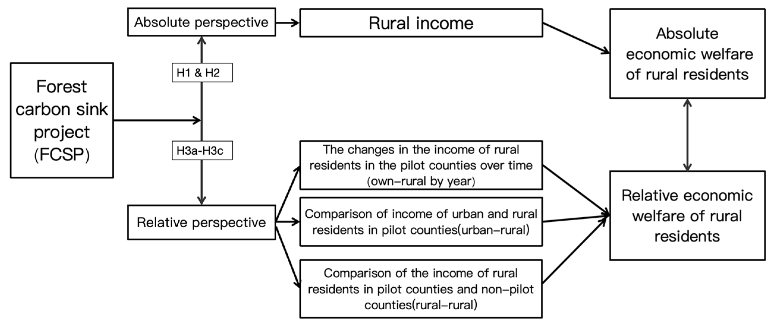
Figure 1.
Theoretical analysis framework. The impact mechanism of rural residents’ economic welfare of forest carbon sink projects from the perspective of absolute and relative.
Figure 1.
Theoretical analysis framework. The impact mechanism of rural residents’ economic welfare of forest carbon sink projects from the perspective of absolute and relative.
3. Methods and Data
3.1. Economic Welfare Measurement Method of Rural Residents from a Relative Perspective
3.1.1. Calculation Methods for Vertical Comparison, Rural-Rural Comparison, and Urban-Rural Comparison
Based on the above theoretical analysis, this study divides the economic welfare of FCSP into four components: absolute income, longitudinal comparison, horizontal inter-rural comparison, and horizontal urban–rural comparison. Absolute income refers to the income of local rural residents; longitudinal comparison measures the difference between the current income of local rural residents and their past income; horizontal inter-rural comparison captures the income gap between local rural residents and those in non-pilot counties; and horizontal urban–rural comparison reflects the income gap between local rural residents and local urban residents.
Drawing on the measurement formulas for individual relative deprivation and intergroup relative deprivation proposed by Ren Guoqiang et al. (2011) [47], Ren Guoqiang et al. (2011) define intergroup relative deprivation as follows: if the overall income distribution is x is the income of different individuals.
According to the definition of relative deprivation by Runciman and Yitzhaki, the relative deprivation of unit is:
At the same time, referring to Li Guoping’s relative income comparison formula [48], if , We list the measurement formulas of vertical comparison, rural-rural comparison, and urban-rural comparison as follows:
Further, we define vertical comparison, horizontal rural-rural comparison and horizontal urban-rural comparison for all counties as follows:
If , Assign V1, V2, V3, V4, V5, V6 to 0;
Among them:
Equation (2) is the longitudinal comparison of county i; indicates the income of rural residents in county i; indicates the income of rural residents in the previous year in county i.
Equation (3) is the horizontal township comparison of county i; indicates the income of rural residents in county i; indicates the average income of rural residents in counties where forest carbon sink projects have not been implemented.
Equation (4) is the horizontal urban-rural comparison of county i; is the same as Equation (3), indicates the income of townspeople in county; indicates the average income of urban residents in all counties.
V1, V2, V3, V4, V5, and V6 are the function expressions of county i vertical comparison, horizontal township comparison, horizontal urban-rural comparison and vertical comparison of all counties, horizontal township comparison, and horizontal urban-rural comparison.
3.1.2. The General Form of the Economic Welfare Function for Residents in Project Areas
Drawing on the utility function form proposed by Boskin [49]:
; where represents the level of personal consumption, represents the average consumption level of all people; is a parameter that reflects the degree of care of an individual about the relative position.
Assume that there are both pilot counties and non-pilot counties for forest carbon sequestration projects, and that each county consists of two types of areas: urban (U) and rural (R). The rural economic welfare function of county i can then be expressed as:
represent the parameters of the weights of relative factors in the utility functions of vertical comparison, horizontal rural-rural comparison, and horizontal urban-rural comparison. represent the basic characteristics of the county.
Furthermore, this study assumes that the rural economic welfare function described above has the following properties:
First, is positively correlated with the economic welfare of county , with diminishing marginal returns.
Second, if , it indicates that the economic welfare of county has increased.
Third, the greater the gap between and , or between and , the lower the economic welfare of county .
Fourth, if are all equal to zero, it means that the rural economic welfare of FCSP pilot counties is determined solely by rural residents’income; otherwise, it is also influenced by other relative factors.
Therefore, the welfare loss of rural areas in FCSP pilot counties caused by longitudinal comparison, horizontal inter-rural comparison, and horizontal urban–rural comparison can be expressed as:
When are all non-zero, and , this indicates that longitudinal comparison, horizontal inter-rural comparison, and horizontal urban–rural comparison are equally important [50].
As shown in Equation (9), The larger its value, the greater the rural economic welfare loss in pilot counties caused by relative factors in FCSP.
3.1.3. The Specific Form of the Economic Welfare Function in Project Areas
Drawing on the utility function form of Clark [50]: , The economic welfare of region can be expressed as:
Logarithmize the above formula:
Then all forest carbon sinks and rural economic benefits are:
Where is the income of rural residents; is the vertical comparison; is the rural comparison, and is the urban-rural comparison.
3.2. An Empirical Model for Analyzing the Impact of FCSP on the Economic Welfare of Rural Residents
To evaluate the impact of FCSP on the economic welfare of rural residents, the single-difference method can be used to compare economic development before and after project implementation. However, since the implementation of FCSP is non-random, using the single-difference method is prone to “selection bias”. A more reliable approach is to apply the difference-in-differences(DID) method to assess the policy effects of the project.
Nevertheless, when implementing DID, if the entire sample is used as the treatment and control groups, the vast geographic span of Sichuan may lead to substantial differences between the two groups, potentially introducing bias into the results. Therefore, this study first employs the propensity score matching(PSM) method to match the samples and then applies the DID method to estimate the net impact of FCSP implementation on the economic welfare of rural residents.
- Propensity Score Matching (PSM)
The propensity score matching (PSM) method is a non-parametric approach that addresses sample self-selection issues by constructing a counterfactual framework, without imposing restrictions on error term distribution, functional form, or other such conditions [51].
The empirical analysis in this study proceeds as follows:
First, Select the characteristic variables Xi, which serve as control variables. Second, Calculate the propensity scores. This study uses a Logit model to estimate the propensity score of county implementing a forest carbon sequestration project(FCSP). The model is specified as follows: ; Where is the policy dummy variable, and represents the control variables.Third, Perform propensity score matching. Common PSM algorithms include nearest neighbor matching, radius matching, and kernel matching. The three methods are subjected to balance tests, and by comparing the density function plots before and after matching as well as the model’s goodness-of-fit, it is found that the nearest neighbor matching method is more appropriate. Therefore, this study adopts the nearest neighbor matching algorithm to conduct one-to-one matching between the treatment group and the control group.
- 2.
- Difference in Difference model (DID)
The difference-in-differences (DID) model is a commonly used policy evaluation method that assesses policy effects by comparing the changes in outcomes between the control group and the treatment group before and after policy implementation. To accurately evaluate the impact of FCSP on the economic welfare of rural residents, this study use DID model, specified as follows:
In Equation (13), is the dependent variable, and is the constant term. indicate whether a county participates in the FCSP; is a dummy variable distinguishing the periods before and after project implementation, is the key explanatory variable measuring whether the carbon sequestration afforestation project is implemented. represents the net impact of FCSP on the economic welfare of rural residents. denotes the control variables, with representing the coefficients of each control variable. captures individual fixed effects that do not vary over time; denotes time fixed effects; is the random disturbance term.
Furthermore, to estimate the dynamic effects of FCSP on the economic welfare of rural residents, the model is specified as follows:
Where is a dummy variable indicating the k-th year after the implementation of the FCSP pilot county project, and measures the policy effect in the k-th year following project implementation.
3.3. Data Description, Data Source and Variable Selection
- Data description
This study selects counties in Sichuan Province, China, as the research area. Located in southwestern China, Sichuan possesses abundant afforestation-suitable land resources and holds an important ecological position. With a forest area ranking among the highest in the country, it has unique advantages for developing FCSP.
Moreover, it has been designated by China as one of the key development areas and among the first pilot regions for the forest carbon sequestration industry. In terms of pilot FCSP implementation, Sichuan has long been at the forefront nationally; its carbon sequestration afforestation projects account for 2 of the 5 CDM projects registered with the Executive Board (EB) of the United Nations Clean Development Mechanism, making Sichuan a key region for FCSP development in China [21].
By the end of 2020, a total of 13 counties in Sichuan had successively implemented FCSP. As shown in the Table 1, these projects were launched between 2004 and 2012, covering three types—CCER, CDM, and VCS—with crediting periods of either 20 or 30 years, and substantial variation in project size.
- 2.
- Data source
Due to data completeness and availability constraints, this study selects samples from the period 2007–2022. Given that data for certain counties are unavailable, and that some counties (districts) such as Qianfeng District of Guang’an City implemented projects after 2007 with incomplete data, 44 counties/districts were excluded from the 183 counties in Sichuan Province. Ultimately, data from 139 counties were retained. The data sources include the China County Statistical Yearbook (various years), the Sichuan Statistical Yearbook, statistical bulletins on the national economic and social development of each county in Sichuan, and government work reports.
- 3.
- Variable selection
Dependent variables. This study employs five indicators as dependent variables: (1)rural residents’ economic welfare without considering relative factors(W1);(2)rural residents’ economic welfare considering relative factors(W2);(3)longitudinal comparison(H-H);(4)horizontal rural-rural comparison(R-R);(5)horizontal urban–rural comparison(U-R). These jointly capture the economic welfare effects of FCSP implementation from both absolute and relative perspectives.
Core explanatory variable. The core explanatory variable is whether the county is an FCSP pilot county in a certain year(DID), which is a binary variable. A value of 1 is assigned if the county has implemented an FCSP, and 0 otherwise.
Control variables. The selection of control variables must satisfy the condition of influencing both rural residents’ income and the implementation of FCSP. On one hand, FCSP are generally implemented in areas with high ecological vulnerability, which are often highly coupled with economically underdeveloped regions [52]. This suggests that the characteristics of local economic development may affect the likelihood of implementing FCSP [21]. Therefore, this study includes whether the county is a poverty-alleviation county (Poverty), whether it is an ethnic county (Ethnic), road mileage per unit of administrative area (Rma), and per capita GDP (Pgdp) as part of the characteristic variables. On the other hand, FCSP sites are generally located in afforestation-suitable barren hills, sandy wasteland, and other afforestation-suitable land [53]. Agricultural production characteristics can indirectly reflect land attributes. Accordingly, this study includes the share of primary industry employment in total employment (Pie), total power of agricultural machinery (Tpam), the ratio of cultivated land area at year-end to total administrative land area (Rcl), fertilizer consumption (Fercon), and grain yield per unit of cultivated land (Gcl) as additional characteristic variables. All variables are listed in Table 2.
4. Empirical Results
4.1. Model Testing
Before proceeding with the main analysis, it is essential to assess the results of the propensity score matching (PSM) through two key evaluations—the balance test and the common support assumption test—to ensure the reliability of the model.
4.1.1. Balance Test
Referring to Chen Qiang, the pstest command is used to conduct the balance test. As shown in Table 3, before propensity score matching, these explanatory variables had a significant impact on whether farmers participated in the FCSP(p-values close to zero). However, after matching, these variables were no longer significant, indicating that the effectiveness of using these characteristic variables to predict farmers’participation in the project had diminished, and the sample satisfied the conditional independence assumption.
4.1.2. Balance Test
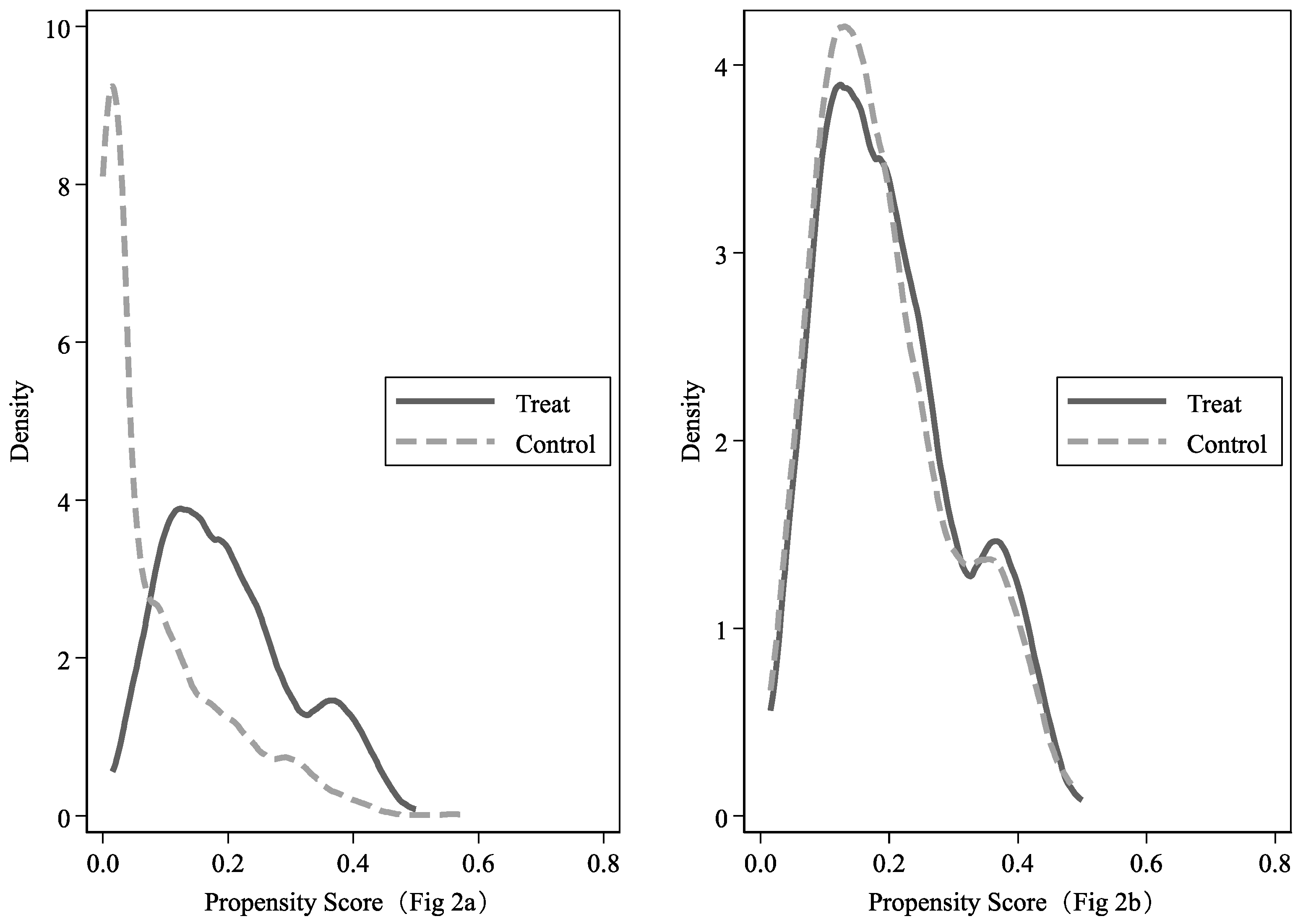
Figure 2 illustrates the distribution of propensity scores (kernel density curves) for the treatment and control groups before and after matching. The vertical axis represents probability density, and the horizontal axis represents propensity score values. Figure (2a) depicts the distribution prior to matching, where the treatment and control groups share minimal overlapping areas. This indicates substantial observable differences between the two groups and suggests that the selection into FCSP implementation is not entirely random across the full sample. Therefore, applying propensity score matching is necessary. Figure (2b) shows the distribution after matching. The kernel density curves of the two groups exhibit a high degree of overlap, indicating that the scores are similar and that few observations were lost during matching. This demonstrates that the matching procedure performed well, yielded representative samples, and eliminated significant differences in covariates between the treatment and control groups.
Figure 2.
The distribution of propensity scores (kernel density curves) for the treatment and control groups before and after matching; Figure 2a is pre-matching kernel density figure; Figure 2b is After-matching kernel density figure.
Figure 2.
The distribution of propensity scores (kernel density curves) for the treatment and control groups before and after matching; Figure 2a is pre-matching kernel density figure; Figure 2b is After-matching kernel density figure.
4.2. The Utility of Rural Residents’Economic Welfare and Welfare Loss Considering Relative Factors
Table 4 reports the annual average values of rural residents’net income, horizontal urban–rural comparison, horizontal inter-rural comparison, and vertical comparison in FCSP pilot counties. Column2 shows that the annual average net income of rural residents in FCSP pilot counties has exhibited a year-by-year upward trend. Column3 shows that the overall trend of the horizontal urban–rural comparison is a gradual decline, indicating that the urban–rural income gap in FCSP pilot counties is narrowing year by year, with continuous improvement in coordinated urban–rural economic development. Column4 presents the horizontal inter-rural comparison, which shows an overall increasing trend over the years. Column5 presents the vertical comparison, which shows that, compared to the previous year, the overall rural residents’income in FCSP pilot counties has been decreasing, suggesting a year-by-year decline in rural residents’economic welfare in these counties.
Based on the above discussion, when relative factors are taken into account, the economic welfare of rural residents declines. This raises the question: how much welfare loss is caused by changes in each relative factor? To address this, a further analysis was conducted.
As previously stated, without considering relative factors, the economic welfare of rural residents in FCSP pilot counties is denoted as W1; when relative factors are considered, it is denoted as W2. Table 5 reports the welfare levels of rural residents in FCSP pilot counties under both scenarios. Column 2 shows that without considering relative factors, rural residents’ economic welfare in FCSP pilot counties exhibits an overall upward trend. Column 3 reveals that when relative factors are considered, economic welfare declines compared to Column 2, although the overall trend remains upward. This indicates that accounting for relative factors results in a reduction in economic welfare. Column 4 further demonstrates that vertical comparison, horizontal inter-rural comparison, and horizontal urban–rural comparison together lead to an average welfare loss of 9.05%.
4.3. Economic Welfare Effects of FCSP on Rural Residents
This study uses the rural residents’ economic welfare without considering relative factors (W1) and with considering relative factors (W2), calculated according to Equation (11), as dependent variables to estimate the net impact of FCSP implementation on rural residents’ economic welfare.
Table 6 presents the results of the average effect test. The empirical findings show that FCSP implementation significantly improves rural residents’ economic welfare from an absolute perspective, with a DID coefficient of 0.111, significant at the 1% level, indicating that welfare increases by approximately 0.111 units after project implementation when relative factors are not considered. However, when relative factors are taken into account, the effect turns significantly negative, with a DID coefficient of –0.119, significant at the 5% level, implying an average welfare loss of 0.119 units due to relative comparisons.
Based on the above empirical results, the implementation of FCSP can effectively improve rural residents’ economic welfare from an absolute perspective. However, when relative factors are taken into account, rural residents’ economic welfare significantly declines. What, then, is the mechanism behind this decline?
To further explain the reasons, this study decomposes rural residents’ economic welfare from a relative perspective into three components: horizontal urban–rural comparison (U–R), horizontal inter-rural comparison (R–R), and vertical comparison (H–H). Using the models specified in Equations (13) and (14), we estimate the welfare effects of FCSP from a relative perspective. The regression results, reported in Table 7, show that FCSP implementation significantly narrows the urban–rural gap, with the U–R index decreasing by 0.094 at the 1% significance level. However, it simultaneously increases inter-rural deprivation, with the R–R index rising by 0.129 at the 1% significance level, and reduces vertical comparison scores, with the H–H index falling by 0.211 at the 1% significance level. The magnitude of the positive effect from narrowing the urban–rural gap is smaller than the combined negative impacts of increased inter-rural deprivation and reduced vertical comparison, ultimately leading to a significant decline in rural residents’ economic welfare when relative factors are considered.
4.4. Dynamic Effects of FCSP on Rural Residents’ Economic Welfare
The above results reflect the average effect of FCSP implementation on rural residents’ economic welfare but do not examine whether this impact exhibits lagged effects or dynamic persistence. In the sample, the 13 treatment counties began implementation in different years—specifically in 2004 and 2010–2012—meaning that policy start dates are not uniform. To eliminate potential confounding influences from other policies enacted in different periods, this study selects as the analysis sample the five counties that began implementation in 2010 and investigates their dynamic effects from 2010 to 2022.Using Equation (14), we test the dynamic effects of FCSP on rural residents’ economic welfare. The empirical results are reported in Table 8, where d1–d13 represent the dynamic effects from 2010 (the year of implementation) to 2022. The results indicate that the implementation of FCSP does not significantly improve rural residents’ economic welfare in the short term, exhibiting a clear lagged effect, with benefits strengthening over time.
The dynamic effect estimates show that under the absolute perspective (W1), coefficients for the first seven periods (d1–d7) after implementation are insignificant, with the first five (d1–d5) being negative (–0.219 in d1, –0.129 in d2). The positive effect emerges in period 8 (d8 = 0.256, significant at the 10% level) and reaches its peak in period 12 (0.375, significant at the 1% level).
Under the relative perspective (W2). The coefficient in period 7 is –0.456 (significant at the 1% level), and those from periods 8 to 12 remain significantly negative (d10 = –0.654, significant at the 1% level; d12 = –0.642, significant at the 1% level), indicating that FCSP substantially reduces rural residents’ welfare during the mid-term when relative factors are considered. By period 13, the coefficient turns positive (0.065) but insignificant, suggesting that the negative influence of relative factors diminishes in the long run.
Overall, the short-term negative effect may stem from the absence of immediate economic returns and potential constraints on agricultural production, leading some part-time farmers to reduce cultivated land without promptly securing non-agricultural employment, thereby lowering welfare in the early years. In the long run, however, FCSP not only improves absolute welfare but also delivers ecological and social benefits that enhance overall utility for participants. Policymakers should therefore prioritize long-term impacts and consider relative welfare effects to achieve a win–win outcome for both the economy and the environment.
4.5. Heterogeneity Analysis
4.5.1. Different Project Cycles
From an investment perspective, the longer the project cycle, the greater the risks and the higher the uncertainty of returns. Therefore, differences in the crediting periods of projects may lead to variations in the economic welfare effects of rural residents participating in forest carbon sequestration projects (FCSP). To investigate this, the existing FCSP are divided into two groups based on their crediting periods: 20 years and 30 years.
Table 9 divides FCSP into two groups based on crediting period length—20 years and 30 years—and examines their average effects on rural residents’ economic welfare. For 20-year projects, the DID coefficient for W1 (without relative factors) is 0.064 and statistically insignificant, indicating no substantial improvement in absolute welfare. When relative factors are considered (W2), the coefficient becomes -0.140, significant at the 10% level, suggesting that shorter-term projects may generate negative welfare effects due to limited economic gains and stronger relative deprivation. In contrast, for 30-year projects, the DID coefficient for W1 is 0.127, significant at the 5% level, showing that longer-term projects significantly enhance absolute welfare. For W2, the coefficient is -0.117, significant at the 10% level; although still negative, the magnitude is smaller than in the 20-year group, implying a weaker adverse effect from relative factors. Overall, longer crediting periods tend to produce stronger positive impacts on rural residents’ economic welfare while mitigating the negative effects of relative deprivation.
To examine the impact of relative factors on the economic welfare of rural residents, the PSM-DID model was applied to estimate the welfare effects of FCSP with different crediting periods from a relative perspective. The results are presented in Table 10. For projects with a 20-year crediting period (Columns 2–4), the DID estimates show that implementation significantly increased horizontal inter-rural comparison (0.127, significant at the 1% level), indicating greater relative deprivation between rural areas, which in turn reduced economic welfare. In contrast, the effects on horizontal urban–rural comparison (-0.001, not significant) and vertical comparison (-0.123, not significant) were not statistically significant.
For projects with a 30-year crediting period (Columns 5–7), FCSP implementation significantly reduced horizontal urban–rural comparison (-0.174, significant at the 1% level), effectively narrowing the urban–rural gap and thus improving economic welfare. However, it also significantly increased horizontal inter-rural comparison (0.138, significant at the 1% level) and significantly reduced vertical comparison (-0.290, significant at the 1% level), both of which exert negative impacts on welfare.
Overall, for 20-year projects, the significant negative welfare effect after accounting for relative factors is mainly due to the increase in inter-rural disparities. For 30-year projects, although the effect remains significantly negative, the coefficient is smaller, suggesting that the positive impact of narrowing the urban–rural gap partially offsets the negative effects arising from increased inter-rural deprivation and reduced vertical comparison.
4.5.2. Different Poverty Attributes
Given that FCSP in Sichuan Province have been piloted in both poverty-alleviated counties and non-poverty counties, this study investigates the differences in their economic welfare effects across rural areas with varying poverty attributes. Table 11 presents the average effect test results of the Forest Carbon Sequestration Project (FCSP) on rural residents’ economic welfare, distinguishing between general counties and poverty-alleviated counties.
For general counties, the DID coefficient for W1 (absolute perspective) is 0.067 and not statistically significant, indicating that FCSP implementation does not significantly affect rural residents’ economic welfare when relative factors are not considered. However, for W2 (relative perspective), the DID coefficient is -0.197 and significant at the 1% level, suggesting that when relative factors are taken into account, FCSP implementation significantly reduces rural residents’ economic welfare in these areas.
For poverty-alleviated counties, the DID coefficients for both W1 (0.026) and W2 (-0.047) are statistically insignificant, implying that FCSP implementation has no measurable effect on rural residents’ economic welfare regardless of whether relative factors are considered. Notably, the negative coefficient for W2 is smaller in magnitude compared to general counties, suggesting a milder reduction in relative welfare for poverty-alleviated counties.
Overall, the results indicate that the adverse relative welfare effect of FCSP implementation is more pronounced in general counties than in poverty-alleviated counties.
Table 12 reports FCSP on rural residents’ economic welfare across general counties and poverty-alleviated counties. In general counties, FCSP implementation has no significant effect on the horizontal urban–rural comparison (U–R). However, it significantly increases horizontal inter-rural disparity (R–R) with a coefficient of 0.132 at the 1% significance level, FCSP may intensify inequality between rural areas. Furthermore, the project significantly reduces vertical comparison scores (H–R) with a coefficient of –0.142 at the 5% significance level, indicating a negative impact on welfare from the perspective of intertemporal comparisons.
In contrast, in poverty-alleviated counties, FCSP significantly narrows the urban–rural gap, as shown by the coefficient of –0.121 for U–R, significant at the 1% level. This improvement in urban–rural equity, however, is accompanied by a significant increase in inter-rural disparity, with the R–R coefficient reaching 0.117 at the 1% significance level. Moreover, the reduction in vertical comparison scores is even more pronounced than in general counties, with an H–R coefficient of –0.277 significant at the 1% level, indicating stronger negative intertemporal welfare effects.
Overall, while poverty-alleviated counties benefit more from the narrowing of the urban–rural gap, the gains are offset by the combined negative effects of widening inter-rural disparities and declining vertical comparison scores.
4.5.3. Different Ethnic Attributes
Given that China is a multi-ethnic country, substantial differences exist in the economic and social development environments between non-ethnic and ethnic regions. Implementing the FCSP in counties with different ethnic attributes may therefore have varying impacts on local economic welfare. Accordingly, this study examines the heterogeneous effects of FCSP on rural economic welfare based on whether a pilot county is classified as an ethnic county.
The results for non-ethnic counties (Columns 2–3) indicate that FCSP implementation significantly improves rural residents’ economic welfare from an absolute perspective. However, when relative factors are considered, the impact becomes statistically insignificant. In contrast, the results for ethnic counties (Columns 4–5) show that FCSP implementation has no significant effect on rural residents’ economic welfare from an absolute perspective, but when relative factors are taken into account, it significantly reduces rural residents’ economic welfare.

Table 13.
The average effect test results of the impact of FCSP of different ethnic on economic welfare of rural residents from a relative perspective.
Table 13.
The average effect test results of the impact of FCSP of different ethnic on economic welfare of rural residents from a relative perspective.
| Non-ethnic country | Ethnic country | |||
| W1 | W2 | W1 | W2 | |
| DID | 0.236*** | 0.019 | -0.062 | -0.284*** |
| (0.047) | (0.084) | (0.060) | (0.069) | |
| _cons | 8.539*** | 7.667*** | 8.244*** | 7.364*** |
| (0.117) | (0.209) | (0.155) | (0.178) | |
| Control | Y | Y | Y | Y |
| Fix_id | Y | Y | Y | Y |
| Fix_year | Y | Y | Y | Y |
| N | 525 | 525 | 654 | 654 |
| R2 | 0.717 | 0.539 | 0.461 | 0.415 |
1 The classification of ethnic and non-ethnic counties is based on the administrative division attributes of the pilot counties. According to the administrative division lists published by the National Bureau of Statistics and local governments, counties designated as “autonomous counties” are classified as ethnic counties, while all others are classified as non-ethnic counties.
Table 14 presents the average effect test results of the impact of FCSP on rural residents’ economic welfare from a relative perspective, differentiated by ethnic attributes. The results for non-ethnic counties (Columns 2–4) indicate that FCSP implementation significantly increases inter-rural comparisons, thereby reducing rural residents’ economic welfare. For ethnic counties (Columns 5–7), the results show that while FCSP implementation can reduce the urban–rural gap, it simultaneously widens inter-rural disparities and lowers vertical comparison scores to a greater extent. Therefore, the primary reason for the significant decline in rural residents’ economic welfare in ethnic counties, when relative factors are considered, is the increase in inter-rural deprivation and the reduction in vertical comparison.
Table 14.
The average effect test results of the impact of FCSP of different ethnic on economic welfare of rural residents from a relative perspective.
Table 14.
The average effect test results of the impact of FCSP of different ethnic on economic welfare of rural residents from a relative perspective.
| Non-ethnic country | Ethnic country | |||||
| U-R | R-R | H-H | U-R | R-R | H-H | |
| DID | 0.025 | 0.130*** | -0.107 | -0.120*** | 0.176*** | -0.234*** |
| (0.025) | (0.031) | (0.107) | (0.026) | (0.027) | (0.055) | |
| _cons | 0.591*** | 0.045 | 0.817*** | 0.722*** | 0.485*** | 0.733*** |
| (0.063) | (0.076) | (0.265) | (0.067) | (0.071) | (0.143) | |
| Control | Y | Y | Y | Y | Y | Y |
| Fix_id | Y | Y | Y | Y | Y | Y |
| Fix_year | Y | Y | Y | Y | Y | Y |
| N | 525 | 525 | 525 | 654 | 654 | 654 |
| R2 | 0.091 | 0.409 | 0.131 | 0.208 | 0.379 | 0.149 |
5. Conclusions and Discussion
5.1. Contributions and INNOVATIONS
5.1.1. Contributions
Based on county-level panel data from Sichuan Province spanning 2007–2022, this study employs a propensity score matching–difference-in-differences (PSM-DID) approach to comprehensively evaluate the impact of Forest Carbon Sequestration Projects (FCSP) on the economic welfare of rural residents from both absolute and relative perspectives.
The results indicate that, from an absolute perspective, FCSP significantly improve rural residents’ income levels. However, from a relative perspective, the combined effects of vertical comparison, urban–rural comparison, and rural–rural comparison offset the positive impact, even leading to significant relative welfare losses. Among these, relative deprivation arising from rural–rural comparison and the decline in vertical comparison are the primary negative drivers, with their adverse effects outweighing the gains from narrowing the urban–rural income gap. In addition, the project effects exhibit a marked time lag: in the short term, increased opportunity costs and production constraints may reduce welfare, while in the medium and long term, absolute welfare continues to improve and the negative effects of relative welfare gradually weaken.
Heterogeneity analysis further reveals that, in terms of project duration, 30-year FCSP deliver greater improvements in absolute welfare than 20-year projects, with relatively lighter negative impacts on relative welfare. In contrast, the 20-year projects exhibit stronger negative effects, mainly due to widening rural–rural disparities. Regarding poverty attributes, FCSP in general counties show no significant absolute effect but a significantly negative relative effect; in poverty-alleviated counties, although FCSP yield notable benefits in narrowing the urban–rural gap, these are accompanied by greater rural–rural disparities and a decline in vertical comparison. In terms of ethnic attributes, non-ethnic counties exhibit a significant absolute positive effect and an insignificant relative effect, with the main issue being the intensification of rural–rural comparisons. Ethnic autonomous counties, on the other hand, show no significant absolute effect but a significantly negative relative effect, with the negative impact likewise driven by the expansion of rural–rural disparities and the decline in vertical comparison.
5.1.2. Innovations
This study provides new empirical evidence on the economic welfare effects of forest carbon sequestration projects (FCSP) in rural China by explicitly distinguishing between absolute and relative perspectives. Unlike most previous research, which tends to focus solely on absolute welfare changes, this paper integrates relative welfare considerations—capturing inter-regional and inter-household comparisons—to more comprehensively evaluate policy outcomes. In addition, by employing the PSM-DID approach, the study addresses selection bias and ensures more robust causal inference. Furthermore, the analysis incorporates heterogeneity dimensions such as crediting period length, poverty attributes, and ethnic attributes, offering a nuanced understanding of how FCSP impacts vary across socio-economic and cultural contexts.
5.2. Limitations
Despite these contributions, the study has several limitations. First, the measurement of rural residents’ economic welfare relies on statistical yearbook data, which may not fully capture informal economic activities or household-level heterogeneity. Second, while the PSM-DID method helps mitigate selection bias, unobserved time-varying factors may still influence the results. Third, the study primarily focuses on Sichuan Province, which, although representative in some respects, may limit the generalizability of the findings to other regions with different economic, environmental, or policy contexts. Finally, the analysis does not explicitly incorporate the potential environmental co-benefits or opportunity costs associated with FCSP, which could further enrich the welfare assessment.
5.3. Future Research Directions
Future research could expand the scope of analysis to include multiple provinces or conduct a nationwide assessment, thereby improving external validity. Micro-level household survey data could be incorporated to better capture individual welfare changes and behavioral responses. Moreover, integrating environmental and social co-benefits into the evaluation framework would provide a more holistic understanding of FCSP impacts. Finally, longitudinal studies with extended post-implementation periods could better capture long-term dynamics and potential lag effects, allowing policymakers to fine-tune project design for sustained economic and ecological benefits.
Funding
National Social Science Fund of China, Youth Program: “Research on the Operation Mechanism and Development Countermeasures of China’s Forest Carbon Sink Trading Market from the Perspective of Non-Carbon Benefits” (Grant No. 23CJY061).
Data Availability Statement
The data used in this study were obtained from the Sichuan Agricultural Statistical Yearbook and statistical data publicly released by the statistical bureaus of districts, counties, and their respective prefecture-level cities in Sichuan Province.
Conflicts of Interest
The authors declare no conflicts of interest.
References
- Qi, Y.; Zhang, Y.; Jia, Y. Research on the Operation Mechanism of Forest Carbon Sink Trading Pilot in China. Issues in Agricultural Economy 2014, 35, 73–79. (In Chinese) [Google Scholar] [CrossRef]
- Li, N.; Yang, Y.; He, Y. Overview of Climate Change and Carbon Sink Forestry. Development Research, 2009, 95-97. (In Chinese). [CrossRef]
- Zhou, J.; Xiao, R.; Zhuang, C.; Deng, Y. Urban Forest Carbon Sink and Its Effect on Offsetting Energy Carbon Emissions—A Case Study of Guangzhou. Acta Ecologica Sinica 2013, 33, 5865–5873. (In Chinese) [Google Scholar] [CrossRef]
- Jindal, R.; Kerr, J. M.; Carter, S. Reducing Poverty Through Carbon Forestry? Impacts of the N’hambita Community Carbon Project in Mozambique. World Development 2012, 40, 2123–2135. [Google Scholar] [CrossRef]
- Chen, C. Forest Carbon Sink and Farmers’Livelihood—A Case Study of the World’s First Forest Carbon Sink Project. World Forestry Research 2010, 23, 15–19. (In Chinese) [Google Scholar] [CrossRef]
- Zeng, W.; Liu, S.; Yang, F.; Fu, X. A Review of Forest Carbon Sink Research from the Perspective of Poverty Alleviation. Issues in Agricultural Economy 2017, 38, 102–109+103. (In Chinese) [Google Scholar]
- Yang, F.; Zeng, W. Review and Prospect of China’s Forest Carbon Sink Market. Resource Development&Market 2014, 30, 603–606. (In Chinese) [Google Scholar]
- Zhu, Z.; Huang, C.; Xu, Z.; Shen, Y.; Bai, J. Analysis of the Impact of Risk Preferences of Forest Farmers in Southern Collective Forest Areas on Carbon Sink Supply Willingness—A Risk Preference Experiment Case in Zhejiang Province. Resources Science 2016, 38, 565–575. (In Chinese) [Google Scholar] [CrossRef]
- Chen, Y.; Zhang, X. Analysis of Factors Affecting the Willingness of Forest Farmers to Participate in Forestry Carbon Sinks—Based on Collective Forest Survey Data in Heilongjiang Province. Forestry Economics 2018, 40, 98–103. (In Chinese) [Google Scholar] [CrossRef]
- Ming, H.; Qi, Y.; Li, Y.; Yu, W. Do Forest Farmers Have the Willingness to Participate in Forestry Carbon Sink Projects? —Taking CDM Forestry Carbon Sink Pilot Project as an Example. Journal of Agrotechnical Economics, 2015, 102-11. (In Chinese). [CrossRef]
- Silva, C. A.; Hudak, A. T.; Vierling, L. A.; Loudermilk, E. L.; O’Brien, J. J.; Hiers, J. K.; Jack, S. B.; Gonzalez-Benecke, C.; Lee, H.; Falkowski, M. J. Imputation of individual longleaf pine(Pinus palustris Mill. ) tree attributes from field and LiDAR data. Canadian journal of remote sensing 2016, 42, 554–573. [Google Scholar] [CrossRef]
- Chen, C. Forest Carbon Sink and Farmers’Livelihood—A Case Study of the World’s First Forest Carbon Sink Project. World Forestry Research 2010, 23, 15–19. (In Chinese) [Google Scholar] [CrossRef]
- Parajuli, P. B. Assessing sensitivity of hydrologic responses to climate change from forested watershed in Mississippi. Hydrological Processes 2010, 24, 3785–3797. [Google Scholar] [CrossRef]
- Ning, K.; Shen, Y.; Zhu, Z. Analysis of Farmers’Cognition of Forest Carbon Sinks and Their Willingness to Manage Carbon Sink Forests—Based on Farmer Surveys in Zhejiang, Jiangxi, and Fujian Provinces. Journal of Beijing Forestry University(Social Sciences) 2014, 13, 63–69. (In Chinese) [Google Scholar] [CrossRef]
- Yang, F.; Zeng, W.; Zhang, W.; Zhuang, T. Forest Farmers’Willingness for Continuous Participation in Forest Carbon Sink Projects and Its Influencing Factors. Scientia Silvae Sinicae 2016, 52, 138–147. (In Chinese) [Google Scholar]
- Gong, R.; Zeng, W. Constraints on Farmers’Participation in Forest Carbon Sink Projects under Government Promotion. Resources Science 2018, 40, 1073–1083. (In Chinese) [Google Scholar] [CrossRef]
- Huang, Z.; Chen, Z.; Chen, Q. Analysis of Factors Affecting Forest Farmers’Willingness to Receive Compensation for Carbon Sink Forest Management—Based on the Theory of Planned Behavior. Forestry Economics 2017, 39, 46–52+91. (In Chinese) [Google Scholar] [CrossRef]
- Richards, K. R.; Stokes, C. A review of forest carbon sequestration cost studies: A dozen years of research. Climatic Change 2004, 63. [Google Scholar] [CrossRef]
- Jack, B. K.; Kousky, C.; Sims, K. Designing payments for ecosystem services: Lessons from previous experience with incentive-based mechanisms. Proceedings of the National Academy of Sciences of the United States of America 2008, 105, 9465–9470. [Google Scholar] [CrossRef] [PubMed]
- Brockmann, H.; Delhey, J.; Welzel, C.; Hao, Y. The China Puzzle: Falling Happiness in a Rising Economy. Journal of Happiness Studies 2009, 10, 387–405. [Google Scholar] [CrossRef]
- Hu, Y.; Zeng, W. Do Carbon Sink Afforestation Projects Promote Local Economic Development? —An Empirical Study Based on County-Level Panel Data in Sichuan Using PSM-DID. China Population, Resources and Environment 2020, 30, 89–98. (In Chinese) [Google Scholar]
- Pagiola, S. Payments for Environmental Services in Costa Rica.2006.
- Hejnowicz, A. P.; Hilary, K.; Rudd, M. A.; Huxham, M. R. Harnessing the climate mitigation, conservation and poverty alleviation potential of seagrasses: prospects for developing blue carbon initiatives and payment for ecosystem service programmes. Frontiers in Marine Science 2017, 2, 32. [Google Scholar] [CrossRef]
- Peng, K. The Social Welfare Effects of Rural-to-Urban Farmland Transfer. PhD Dissertation, Huazhong Agricultural University, 2008. (In Chinese).
- Grieg-Gran, M.; Porras, I.; Wunder, S. How can market mechanisms for forest environmental services help the poor? Preliminary lessons from Latin America. World Development 2005, 33, 1511–1527. [Google Scholar]
- Parajuli; Rajan; Lamichhane; Dhananjaya; Joshi; Omkar. Does Nepal’s community forestry program improve the rural household economy? A cost-benefit analysis of community forestry user groups in Kaski and Syangja districts of Nepal. J FOREST RES-JPN.
- Mchenry, M. P. Agricultural bio-char production, renewable energy generation and farm carbon sequestration in Western Australia: Certainty, uncertainty and risk. Agriculture Ecosystems&Environment 2009, 129, 1–7. [Google Scholar]
- Brandth, B.; Haugen, M. S. Farm diversification into tourism-Implications for social identity? Journal of Rural Studies 2011, 27, 35–44. [Google Scholar] [CrossRef]
- Konu, H. Developing a forest-based wellbeing tourism product together with customers–An ethnographic approach. Tourism Management 2015, 49, 1–16. [Google Scholar] [CrossRef]
- Grabowski, Z. J.; Chazdon, R. L. Beyond carbon: Redefining forests and people in the global ecosystem services market. Sapiens 2012, 5. [Google Scholar]
- Ferraro, P. J.; Hanauer, M. M.; Miteva, D. A.; Nelson, J. L.; Pattanayak, S. K.; Nolte, C.; Sims, K. R. E. Estimating the impacts of conservation on ecosystem services and poverty by integrating modeling and evaluation. Proc Natl Acad Sci U S A 2015, 112, 7420–7425. [Google Scholar] [CrossRef]
- Yang, H.; Zeng, S.; Zeng, W.; Yang, F. Ecological Compensation for Forest Carbon Sink Afforestation in China Based on Hicks Analysis—Taking Land Use Change from”Pastureland to Carbon Sink Forest Land”as an Example. Science and Technology Management Research 2016, 36, 221–227. (In Chinese) [Google Scholar]
- Li, J.; Ming, H.; Yu, W. Comparative Analysis of the Implementation of Forestry Carbon Sink Projects in Sichuan Province. Journal of Sichuan Agricultural University 2015, 33, 332–337. (In Chinese) [Google Scholar] [CrossRef]
- Asquith, N. M.; Ríos, M. T. V.; Smith, J. Can Forest-protection carbon projects improve rural livelihoods? Analysis of the Noel Kempff Mercado climate action project, Bolivia. Mitigation&Adaptation Strategies for Global Change 2002, 7, 323–337. [Google Scholar]
- You, L.; Huo, X.; Du, W. Absolute Income, Social Comparison and Farmers’Subjective Well-being—An Empirical Study Based on Two Entire Villages in Shaanxi. Journal of Agrotechnical Economics, 2018, 111-125. (In Chinese). [CrossRef]
- Li, T.; Fang, M.; Fu, L.; Jin, X. Objective Relative Income and Subjective Economic Status: Empirical Evidence from a Collectivist Perspective. Economic Research 2019, 54, 118–133. (In Chinese) [Google Scholar]
- Oswald, A. J. HAPPINESS AND ECONOMIC PERFORMANCE. The Economic Journal 1997. [CrossRef]
- Duesenberry, J. S. Income, Saving, and the Theory of Consumer Behavior. Review of Economics&Statistics 1949, 33, 111. [Google Scholar]
- Parijat, P.; Bagga, S. Victor Vroom’s expectancy theory of motivation–An evaluation. International Research Journal of Business and Management 2014, 7, 1–8. [Google Scholar]
- Gong, R.; Cheng, R.; Zeng, M.; Zeng, W. Analysis of Poverty Alleviation Effect of Forest Carbon Sink Based on Farmers’Perception. South China Journal of Economics, 2019, 84-96. (In Chinese). [CrossRef]
- Festinger, L. A theory of social comparison processes. Human relations 1954, 7, 117–140. [Google Scholar] [CrossRef]
- Jindal, R.; Swallow, B.; Kerr, J. Forestry-based carbon sequestration projects in Africa: Potential benefits and challenges. Natural Resources Forum 2010. [CrossRef]
- Wu, W.; Sun, T.; Xu, Q.; Cao, X. Impact and Implications of Forestry Carbon Sink Policies on Increasing Forest Carbon. Forestry Economics Issues 2022, 42, 659–665. (In Chinese) [Google Scholar]
- Du, J. The Structural Logic and Evolution of the Urban-Rural Development Gap and the Alienation of Environmental Interest Distribution in China. Research of Agricultural Modernization 2013, 34, 564–568. (In Chinese) [Google Scholar]
- Teng, F.; Lü, D.; Chai, H. Research on the Economic Development Path of Forestry Carbon Sink in Heilongjiang Province Based on PEST-SWOT Matrix. Sustainability 2019, 9, 9. (In Chinese) [Google Scholar]
- Zeng, W.; Cheng, Y.; Yang, F. Research on the Evaluation Index System of Forest Carbon Sink Poverty Alleviation Performance Based on CDM Afforestation and Reforestation Projects. Journal of Nanjing Forestry University: Natural Sciences 2018, 42, 9. (In Chinese) [Google Scholar]
- Ren, G.; Shang, J. A Method for Subgroup Decomposition of Gini Coefficient Based on Relative Deprivation Theory. The Journal of Quantitative&Technical Economics 2011, 28, 103–114. (In Chinese) [Google Scholar] [CrossRef]
- Li, G.; Shi, H. The Economic Welfare Effect of Grain-for-Green Compensation from a Comparative Perspective—Based on an Empirical Study of79Grain-for-Green Counties in Shaanxi Province. Economic Geography 2017, 37, 146–155. (In Chinese) [Google Scholar] [CrossRef]
- Boskin, M. J.; Eytan, S. Optimal Redistributive Taxation When Individual Welfare Depends Upon Relative Income. Quarterly Journal of Economics 1978, 589–601. [Google Scholar] [CrossRef]
- Clark, A.; Frijters, P.; Shields, M. A. Relative Income, Happiness and Utility: An Explanation for the Easterlin Paradox and Other Puzzles. Social Science Electronic Publishing.
- Dehejia, R. H.; Wahba, S. Propensity Score-Matching Methods for Nonexperimental Causal Studies. Review of Economics and Statistics 2002, 84, 151–161. [Google Scholar] [CrossRef]
- Chen, R. Analysis of the Coordinated Development of Agricultural Ecology and Economic System in Southwest China. China Agricultural Resources and Regional Planning 2018, 39, 54–57. (In Chinese) [Google Scholar]
- Chen, D. Research on the Construction of Forestry Carbon Sink Market in Heilongjiang Province. Master’s Thesis, Northeast Forestry University, 2014. (In Chinese).
- Chen, Q. Advanced Econometrics and Stata Applications; Beijing: Higher Education Press: 2014; 2nd Edition, pp.542-559. (In Chinese).
Table 1.
Basic Information of Implementation Counties of Carbon Sequestration Afforestation Project in Sichuan Province.
Table 1.
Basic Information of Implementation Counties of Carbon Sequestration Afforestation Project in Sichuan Province.
| County | Project Type | Project Name | Year of Implementation | Poverty alleviation county | Ethnic county | Project cycle | Area/hm2 |
| Mianning | CCER | Audi Panda Habitat has multiple benefits | 2012 | 0 | 1 | 30 | 153.4 |
| Jinyang | CCER | Forest restoration and afforestation carbon sink project | 2012 | 1 | 1 | 30 | 181.7 |
| Lixian | CDM | Afforestation and reforestation project of degraded land in northwest Sichuan, China | 2004 | 0 | 1 | 20 | 747.8 |
| Maoxian | CDM | 2004 | 0 | 1 | 20 | 234.9 | |
| Beichuan | CDM | 2004 | 0 | 0 | 20 | 200.2 | |
| Qingchuan | CDM | 2004 | 0 | 0 | 20 | 190.6 | |
| Ganluo | CDM | 2010 | 1 | 1 | 30 | 924.3 | |
| Yuexi | CDM | Novartis Southwest Degraded Land Afforestation and Reforestation Project | 2010 | 1 | 1 | 30 | 1245.0 |
| Meigu | CDM | 2010 | 1 | 1 | 30 | 731.6 | |
| Zhaojue | CDM | 2010 | 1 | 1 | 30 | 441.8 | |
| Leibo | CDM | 2010 | 1 | 1 | 30 | 854.1 | |
| Yingjing | VCS | Reforestation project in Xingjing County, Sichuan Province | 2011 | 0 | 0 | 30 | 159.2 |
1 CCER is China’s domestic certified emission reduction mechanism for the national voluntary carbon market. CDM, under the Kyoto Protocol and managed by the UN, serves the international compliance market. VCS, run by Verra, is a global voluntary standard for carbon credits used in voluntary carbon markets; 2 Whether it is a poverty-alleviation county and whether it is an ethnic county, with 1 indicating “yes” and 0 indicating “no.”.
Table 2.
Variable selection and explanation.
| Variable | Name | Definition | Variable Description | Mean | SE |
| Depenent variables |
W1 | Economic welfare without considering relative factors | Equation (11) θ1=θ2=θ3=0 | 9.010 | 0.640 |
| W2 | Economic welfare considering relative factors | Equation (11) θ1=θ2=θ3=1/3 | 8.550 | 0.840 | |
| H-H | Vertical comparison | V1, Equation (2) | 0.560 | 0.220 | |
| R-R | Horizontal inter-rural comparison | V2, Equation (3) | 0.030 | 0.330 | |
| U-R | Horizontal urban–rural comparison | V3, Equation (4) | 1.260 | 0.740 | |
| Core explanatory variable. |
DID | Whether a county is an FCSP pilot county | Yes=1, No=0 | 0.090 | 0.290 |
| Controls | Poverty | Whether a county is a poverty-alleviation county | Yes=1, No=0 | 0.240 | 0.430 |
| Ethnic | Whether a county is an ethnic county | Yes=1, No=0 | 0.360 | 0.480 | |
| Pgdp | Per capita GDP | Per capita GDP of each county (unit: CNY) | 29105.000 | 19965.000 | |
| Pie | Share of primary industry employment in total employment | Ratio of primary industry employment to total employment | 0.520 | 0.180 | |
| Tpam | Total power of agricultural machinery | Total power of machinery used in agriculture, forestry, animal husbandry, and fishery (unit: 10,000 kW) | 22.450 | 17.970 | |
| Rcl | Ratio of cultivated land area to total administrative land area | Cultivated land area at year-end (hectares) divided by total administrative land area (hectares) | 0.210 | 0.390 | |
| Fercon | Fertilizer consumption | Annual fertilizer consumption (unit: tonnes) | 13398.000 | 12318.000 | |
| Gcl | Grain yield per unit of cultivated land | Total grain output (tonnes) divided by cultivated land area at year-end (hectares), unit: tonnes/hectare | 1.660 | 0.620 | |
| Rma | Road mileage per unit of administrative area | Road mileage (km) divided by total administrative area (hectares), unit: km/hectare | 1.030 | 0.710 |
1 In the regression analysis, per capita GDP and Fercon was logarithmicized.
Table 3.
Balancing test.
| Variable | Matched & Unmatched | Mean | Bias(%) | Reduct(%) | T-test | ||
| Treated | Control | |bias| | t | p>|t| | |||
| Poverty | U | 0.425 | 0.221 | 44.500 | 6.190 | 0.000 | |
| M | 0.425 | 0.346 | 17.100 | 61.600 | 1.520 | 0.129 | |
| Ethnic | U | 0.665 | 0.333 | 70.200 | 9.030 | 0.000 | |
| M | 0.665 | 0.696 | -6.500 | 90.700 | -0.620 | 0.534 | |
| Pgdp | U | 23995.000 | 29552.000 | -30.200 | -3.580 | 0.000 | |
| M | 23995.000 | 25914.000 | -10.400 | 65.500 | -0.950 | 0.344 | |
| Pie | U | 0.623 | 0.511 | 69.400 | 8.300 | 0.000 | |
| M | 0.623 | 0.614 | 5.400 | 92.300 | 0.520 | 0.605 | |
| Tpam | U | 9.884 | 23.546 | -101.400 | -9.960 | 0.000 | |
| M | 9.884 | 9.016 | 6.400 | 93.600 | 1.400 | 0.162 | |
| Rcl | U | 0.069 | 0.111 | -28.500 | -2.750 | 0.006 | |
| M | 0.069 | 0.058 | 8.100 | 71.400 | 0.490 | 0.622 | |
| Fercon | U | 7274.200 | 13934.000 | -70.800 | -7.010 | 0.000 | |
| M | 7274.200 | 6955.300 | 3.400 | 95.200 | 0.500 | 0.616 | |
| Gcl | U | 1.451 | 1.682 | -46.300 | -4.830 | 0.000 | |
| M | 1.451 | 1.325 | 25.200 | 45.500 | 2.390 | 0.018 | |
| Rma | U | 0.684 | 1.062 | -64.300 | -6.900 | 0.000 | |
| M | 0.684 | 0.624 | 10.200 | 84.200 | 1.260 | 0.209 | |
1 Matching algorithm: Propensity scores were estimated using a Logit model, and counties in the treatment group were matched to counties in the control group using 1:1 nearest neighbor matching; 2 Balance test method: The pstest command in Stata was used to assess covariate balance before and after matching, reporting mean bias, bias reduction (%), and t-test p-values. 3 Variable definitions: See Table 2 for definitions of all covariates.
Table 4.
Economic welfare utility of rural residents in forest carbon sink pilot counties.
| year | Mean_Income | U_R | R_R | H_H |
| 2007 | 2633.692 | 0.669 | 0.251 | 1.000 |
| 2008 | 2970.923 | 0.687 | 0.281 | 1.098 |
| 2009 | 3214.923 | 0.712 | 0.263 | 0.937 |
| 2010 | 3789.692 | 0.700 | 0.265 | 1.119 |
| 2011 | 4567.600 | 0.672 | 0.273 | 0.840 |
| 2012 | 5319.892 | 0.668 | 0.270 | 0.967 |
| 2013 | 6109.610 | 0.650 | 0.263 | 0.968 |
| 2014 | 6938.622 | 0.629 | 0.272 | 0.914 |
| 2015 | 8358.538 | 0.569 | 0.256 | 0.862 |
| 2016 | 9218.692 | 0.560 | 0.252 | 0.878 |
| 2017 | 10168.230 | 0.551 | 0.248 | 0.936 |
| 2018 | 11227.300 | 0.543 | 0.242 | 0.889 |
| 2019 | 9968.923 | 0.363 | 0.273 | 0.799 |
| 2020 | 10889.462 | 0.349 | 0.286 | 0.800 |
| 2021 | 11866.154 | 0.351 | 0.301 | 0.840 |
| 2022 | 12904.538 | 0.367 | 0.318 | 0.804 |
Table 5.
Absolute Welfare, Relative Welfare and Welfare Loss.
| year | W1 | W2 | u |
| 2007 | 7.854 | 7.355 | 0.068 |
| 2008 | 7.958 | 7.493 | 0.062 |
| 2009 | 8.054 | 7.543 | 0.068 |
| 2010 | 8.220 | 7.769 | 0.058 |
| 2011 | 8.403 | 7.859 | 0.069 |
| 2012 | 8.555 | 8.055 | 0.062 |
| 2013 | 8.694 | 8.153 | 0.066 |
| 2014 | 8.823 | 8.147 | 0.083 |
| 2015 | 9.009 | 8.176 | 0.102 |
| 2016 | 9.108 | 8.265 | 0.102 |
| 2017 | 9.207 | 8.381 | 0.099 |
| 2018 | 9.308 | 8.464 | 0.100 |
| 2019 | 9.149 | 8.090 | 0.131 |
| 2020 | 9.227 | 8.155 | 0.131 |
| 2021 | 9.302 | 8.342 | 0.115 |
| 2022 | 9.374 | 8.280 | 0.132 |
| Average | 8.7653 | 8.0329 | 0.0905 |
Table 6.
Average effect test results of the impact of FCSP on rural residents’ economic welfare.
| W1 | W2 | |
| DID | 0.111*** | -0.119** |
| (0.039) | (0.050) | |
| Poverty | -0.043 | -0.322*** |
| (0.036) | (0.046) | |
| Ethnic | 0.117** | 0.249*** |
| (0.047) | (0.059) | |
| Pgdp | 0.013*** | 0.012*** |
| (0.001) | (0.001) | |
| Pie | 0.228* | 0.433*** |
| (0.123) | (0.157) | |
| Tpam | 0.016*** | 0.021*** |
| (0.003) | (0.003) | |
| Rcl | 0.506** | 1.687*** |
| (0.237) | (0.302) | |
| Fercon | -0.138 | -0.462 |
| (0.152) | (0.173) | |
| Gcl | -0.155*** | -0.072* |
| (0.033) | (0.042) | |
| Rma | 0.151*** | 0.172*** |
| (0.024) | (0.031) | |
| _cons | 8.031*** | 7.141*** |
| (0.105) | (0.134) | |
| Fix_id | Y | Y |
| Fix_year | Y | Y |
| N | 1179 | 1179 |
| R2 | 0.474 | 0.418 |
1 Standard deviation in parentheses; 2 And *,**,*** represent 10%, 5%, and 1% saliency levels; 3 The model controls for fixed effects of time and individuals.
Table 7.
The average effect test results of the economic welfare effect of rural residents of FCSP from a relative perspective.
Table 7.
The average effect test results of the economic welfare effect of rural residents of FCSP from a relative perspective.
| U-R | R-R | H-H | |
| DID | -0.094*** | 0.129*** | -0.211*** |
| (0.018) | (0.020) | (0.048) | |
| _cons | 0.800*** | 0.379*** | 0.772*** |
| (0.047) | (0.052) | (0.128) | |
| Control | Y | Y | Y |
| Fix_id | Y | Y | Y |
| Fix_year | Y | Y | Y |
| N | 1179 | 1179 | 1179 |
| R-sq | 0.165 | 0.391 | 0.175 |
1 Standard deviation in parentheses; 2 And *,**,*** represent 10%, 5%, and 1% saliency levels; 3 The model has added fixed effects of control variables, individuals and time.
Table 8.
Test results of the dynamic effect of FCSP on the economic welfare of rural residents.
| W1 | W2 | |
| d1 | -0.219 | -0.090 |
| (0.169) | (0.213) | |
| d2 | -0.129 | 0.006 |
| (0.169) | (0.213) | |
| d3 | -0.036 | -0.109 |
| (0.169) | (0.213) | |
| d4 | -0.116 | -0.259 |
| (0.133) | (0.167) | |
| d5 | -0.058 | -0.255 |
| (0.132) | (0.167) | |
| d6 | 0.032 | -0.196 |
| (0.132) | (0.166) | |
| d7 | 0.188 | -0.456*** |
| (0.132) | (0.165) | |
| d8 | 0.256* | -0.397** |
| (0.132) | (0.166) | |
| d9 | 0.241* | -0.389** |
| (0.132) | (0.165) | |
| d10 | 0.249* | -0.654*** |
| (0.132) | (0.165) | |
| d11 | 0.288** | -0.582*** |
| (0.132) | (0.165) | |
| d12 | 0.375*** | -0.642*** |
| (0.143) | (0.179) | |
| d13 | 0.353** | -0.065 |
| (0.150) | (0.189) | |
| _cons | 7.957*** | 6.922*** |
| (0.106) | (0.135) | |
| Control | Y | Y |
| Fix_id | Y | Y |
| Fix_year | Y | Y |
| N | 1179 | 1179 |
| R2 | 0.484 | 0.446 |
Table 9.
The average effect test results of the impact of FCSP on the economic welfare of rural residents in different periods.
Table 9.
The average effect test results of the impact of FCSP on the economic welfare of rural residents in different periods.
| 20-years | 30-years | |||
| W1 | W2 | W1 | W2 | |
| DID | 0.064 | -0.140* | 0.127** | -0.117* |
| (0.061) | (0.077) | (0.054) | (0.070) | |
| _cons | 7.933*** | 7.015*** | 7.890*** | 6.966*** |
| (0.117) | (0.149) | (0.111) | (0.143) | |
| Control | Y | Y | Y | Y |
| Fix_id | Y | Y | Y | Y |
| Fix_year | Y | Y | Y | Y |
| N | 1056 | 1056 | 1099 | 1099 |
| R2 | 0.467 | 0.426 | 0.495 | 0.436 |
1 The distinction between20-year and30-year crediting periods is based on the crediting duration specified in the Project Design Document(PDD). Twenty-year crediting period projects are often implemented earlier, with shorter crediting durations and renewal uncertainties, whereas30-year crediting period projects have longer crediting periods that can provide more stable long-term returns.
Table 10.
The average effect test results of the impact of FCSP on the economic welfare of rural residents in different accounting periods from the relative perspective.
Table 10.
The average effect test results of the impact of FCSP on the economic welfare of rural residents in different accounting periods from the relative perspective.
| 20-years | 30-years | |||||
| U-R | R-R | H-H | U-R | R-R | H-H | |
| DID | -0.001 | 0.127*** | -0.123 | -0.174*** | 0.138*** | -0.290*** |
| (0.027) | (0.030) | (0.075) | (0.024) | (0.028) | (0.068) | |
| _cons | 0.740*** | 0.412*** | 0.687*** | 0.736*** | 0.435*** | 0.653*** |
| (0.052) | (0.059) | (0.145) | (0.049) | (0.057) | (0.140) | |
| Control | Y | Y | Y | Y | Y | Y |
| Fix_id | Y | Y | Y | Y | Y | Y |
| Fix_year | Y | Y | Y | Y | Y | Y |
| N | 1056 | 1056 | 1056 | 1099 | 1099 | 1099 |
| R2 | 0.157 | 0.358 | 0.154 | 0.190 | 0.402 | 0.186 |
Table 11.
The average effect test results of the impact of FCSP of different poverty attributes on economic welfare of rural residents.
Table 11.
The average effect test results of the impact of FCSP of different poverty attributes on economic welfare of rural residents.
| General County | Poverty alleviation counties | |||
| W1 | W2 | W1 | W2 | |
| DID | 0.067 | -0.197*** | 0.026 | -0.047 |
| (0.054) | (0.070) | (0.055) | (0.069) | |
| _cons | 7.961*** | 6.912*** | 8.104*** | 7.674*** |
| (0.133) | (0.173) | (0.165) | (0.207) | |
| Control | Y | Y | Y | Y |
| Fix_id | Y | Y | Y | Y |
| Fix_year | Y | Y | Y | Y |
| N | 831 | 831 | 348 | 348 |
| R-sq | 0.471 | 0.418 | 0.627 | 0.437 |
1 The distinction between general counties and poverty-alleviated counties is based on the official classification by the Sichuan Provincial Government. Poverty-alleviated counties refer to counties that were officially removed from the national poverty list under China’s targeted poverty alleviation program before the implementation of the FCSP. General counties are those without such poverty-alleviation designation during the study period.
Table 12.
The average effect test results of the impact of FCSP of different poverty attributes on economic welfare of rural residents from a relative perspective.
Table 12.
The average effect test results of the impact of FCSP of different poverty attributes on economic welfare of rural residents from a relative perspective.
| General County | Poverty alleviation counties | |||||
|---|---|---|---|---|---|---|
| U-R | R-R | H-R | U-R | R-R | H-R | |
| DID | -0.030 | 0.132*** | -0.142** | -0.121*** | 0.117*** | -0.277*** |
| (0.023) | (0.028) | (0.067) | (0.030) | (0.023) | (0.075) | |
| _cons | 0.687*** | 0.422*** | 0.654*** | 0.970*** | 0.319*** | 0.759*** |
| (0.058) | (0.069) | (0.166) | (0.091) | (0.068) | (0.223) | |
| Control | Y | Y | Y | Y | Y | Y |
| Fix_id | Y | Y | Y | Y | Y | Y |
| Fix_year | Y | Y | Y | Y | Y | Y |
| N | 831 | 831 | 831 | 348 | 348 | 348 |
| R-sq | 0.164 | 0.355 | 0.162 | 0.335 | 0.316 | 0.155 |
Disclaimer/Publisher’s Note: The statements, opinions and data contained in all publications are solely those of the individual author(s) and contributor(s) and not of MDPI and/or the editor(s). MDPI and/or the editor(s) disclaim responsibility for any injury to people or property resulting from any ideas, methods, instructions or products referred to in the content. |
© 2025 by the authors. Licensee MDPI, Basel, Switzerland. This article is an open access article distributed under the terms and conditions of the Creative Commons Attribution (CC BY) license (https://creativecommons.org/licenses/by/4.0/).
Copyright: This open access article is published under a Creative Commons CC BY 4.0 license, which permit the free download, distribution, and reuse, provided that the author and preprint are cited in any reuse.


