
Submitted:
22 August 2025
Posted:
25 August 2025
You are already at the latest version
Abstract
Biplot methods allow for the simultaneous representation of rows and columns of a data matrix. Classical biplots were developed for continuous data in connection with Principal Components Analysis (PCA). More recently extensions for binary or nominal have been developed. The techniques have been named "Logistic biplots" (LB) because are based on logistic rather than linear responses. None of them are still adequate for ordinal data. In this paper we extend biplot methodology to ordinal data. The resulting method is termed “ordinal logistic biplot” (OLB). Row scores are computed to have ordinal logistic responses along the dimensions and column parameters produce logistic response surfaces that, projected onto the space spanned by the row scores, define a linear biplot. A proportional odds model is used. We study the geometry of such a representation and construct computational algorithms, based on an alternated gradient descent procedure, for estimating model parameters and calculating prediction directions for visualization. We understand the proposed methods as exploratory to reveal interesting patterns in data sets. The main theoretical results are applied to the study of job satisfaction of doctorate (PhD) holders in Spain.
Keywords:
biplot
; multivariate ordinal data
; gradient descent
1. Introduction
The Biplot method [9,19], allows for simultaneous representation of the I rows and J columns of a data matrix , in reduced dimensions, where rows usually correspond to individuals, objects or samples and columns to a set of variables measured on them. Classical Biplot methods are a graphical representation of a Principal Components Analysis (PCA) or Factor Analysis (FA) that are used to obtain linear combinations that successively maximize the extracted variability. From another point of view, Classical Biplots can be obtained from alternated regressions and calibrations in [14]. This approach is essentially an alternated least squares algorithm.
In the context multivariate analysis, biplots are not that popular, although principal components analysis still are. The reason for this is that biplots are probably not well understood and its properties not well explained and also because some lack of connection between the statistical and applied frameworks. We think that every time a principal components analysis is used to analyse data, a biplot could improve significantly such analysis.
For data with distributions from the exponential family, [11] describes bilinear regression as a method to estimate biplot parameters, but the procedure have never been implemented and the geometrical properties of the resulting representations have never been studied in detail. [6] proposes Principal Components Analysis for binary data based on an alternate procedure in which each iteration is performed using iterative majorization and [25] extends the procedure for sparse data matrices, none of those describe the associated biplot. [33] propose a biplot based on logistic responses called “Logistic Biplot” that is linear, and study the geometry of this kind of biplots and uses a estimation procedure that is slightly different from Gabriel’s method. A heuristic version of the procedure for large data matrices in which scores for individuals are calculated with an external procedure as Principal Coordinates Analysis is described in [8]. Method is called “External Logistic Biplot”. Binary Logistic Biplots have been successfully applied to different data sets, see for example, [5,8,16,31] or [17]. More recently, [30] have proposed some additional algorithms to calculate the parameters of the logistic principal components and [1] an algorithm for the biplot.
For nominal data, [22] proposed a biplot representation based on convex prediction regions for each category of a nominal variable. An alternated algorithm is used for the parameter estimation. In Section 2, biplots for continuous, binary and, in lesser extent, nominal variables are described.
Linear, binary or nominal logistic biplots are not adequate when data are ordinal and techniques as CATPCA or IRT for ordinal items can be used instead. The first represents rows and columns of the data matrix in a biplot and the second does not usually have a graphical representation. In Section 3 we extend the logistic biplot to ordinal data. A draft of this extension was already publish in a repository [35]. The resulting method is termed “ordinal logistic biplot” (OLB). Row scores are computed to have ordinal logistic responses along the dimensions and column parameters produce logistic response surfaces that, projected onto the space spanned by the row scores, define a linear biplot. A proportional odds model is used, obtaining a multidimensional model similar to a graded response model in the IRT framework. We study the geometry of such a representation and construct computational algorithms for estimating the model parameters and calculating the prediction directions (or axes) used for visualization on the biplot. Ordinal logistic biplots extend both CATPCA and IRT in the sense that gives a graphical representation for IRT similar in some way to the biplot for CATPCA. The algorithm is based on an alternated gradient descent method.
In Section 4 the main results are applied to the study of job satisfaction of doctorate (PhD) holders in Spain. Holders of doctorate degrees or other research qualifications are crucial to the creation, commercialization and dissemination of knowledge and to innovation. The proposed methods are used to extract useful information from the Spanish data from the international ’Survey on the careers of doctorate holders (CDH)’, jointly carried out by Eurostat, the Organization for Economic Co-operation and Development (OECD) and UNESCO’s Institute for Statistics (UIS).
2. Biplot for Continuous, Binary or Nominal Data
In this section we describe the biplot for continuous, binary and nominal data, being the first two treated in a greater extent because of the closer relation to the proposal of this paper.
2.1. Linear biplot for continuous data
Let be a data matrix containing the measures of J variables on I individuals. The S-dimensional principal components (biplot) model is formulated as:
or in matrix form
where is a vector of constants. can be estimated beforehand and contains the column means (), the scores and the loadings are matrices of rank S with I and J rows respectively, and is a matrix of errors or residuals. Then
In practice we avoid the constants by centring the data matrix. The reduced rank approximation of the centred data matrix is
is usually obtained from its singular value decomposition (SVD),
where contains the eigenvectors of , the eigenvectors of and is a diagonal matrix containing the non-zero eigenvalues of both matrices that are the same. The SVD is closely related to the principal components.
We can choose and in different ways, using the first S columns of the matrices in the SVD, for example,
contains the scores on the principal components and are used for visualization on a scattergram, contains the coefficients of the principal components. This is called a JK-Biplot or RMP-Biplot by [9].
Another possible choice is
contains the factor loadings and the standardized factor scores. If the columns of are standardized, a contains the correlations of the observed variables and the principal components. This is called a GH-Biplot or CMP-Biplot by [9].
Normally the scores in equation 6 are used for visualization od the individuals and the loadings or correlations in 7 to interpret the indirect relation to the components in a process called reification.
The joint representation is called a biplot because simultaneously plots the individuals and variables using the rows of and as markers, in such a way that the inner product approximates the element as close as possible.
If we consider the row markers as fixed and the data matrix previously centred, the column markers can be computed by regression trough the origin:
In the same way, fixing , can be obtained as:
Alternating the steps (8) and (9) the product converges to the same subspace generated by the SVD of the centred data matrix. Regression step in equation (8) adjusts a separate linear regression for each column (variable) and interpolation step in equation (9), interpolates an individual using the column markers as reference. The procedure is in some way a kind of EM-algorithm in which the regression step is the maximization part and the interpolation step is the expectation part. An extension for frequency matrices can be found in [13]. In summary, the expected values on the original data matrix are obtained on the biplot using a simple scalar product, that is, projecting the point onto the direction defined by . This is why row markers are usually represented as points and column markers as vectors (also called biplot axis by [19]).
The biplot axis can be completed with scales to predict individual values of the data matrix. To find the point on the biplot direction, that predicts a fixed value of the observed variable when an individual point is projected, we look for the point lies on the biplot axis, i. e. that verifies
and
Solving for x and y, we obtain
and
or
Therefore, the unit marker for the j-th variable is computed by dividing the coordinates of its corresponding marker by its squared length, several points for specific values of can be labelled to obtain a reference scale. If data are centred then and labels can be calculated by adding the average to the value of (). The resulting representation will be like the one shown in Figure 1. The data for the representation was used to illustrate a biplot by [10].
Data contains the consumption of different types of proteins at different European countries. The aim is to detect groups of countries with similar behaviours and the variables responsible for them.
The biplot allows for the direct interpretation of the relations among rows and columns rather than the indirect relation trough the principal components.
If the expected values of the biplot in reduced dimension , the global goodness of fit is the amount of variability accounted by the prediction, that is,
Even for matrices in which we obtain a good global fit, there may be some columns whose information is not accounted in the plot. Goodness of fit for each column is
where ÷ means the element by element operation. The quantity is also the R-Squared of the regression of each column of on as in equation 8. We call that quantity quality of representation of the variable. [18] call this quantity predictiveness of the column. The measures are used to identify which variables are most related to the representation or the variables whose information is preserved on the biplot. If two dimensions are not enough to account for the desired information, additional components can be used and qualities can be calculated adapting equations 10 and 11 to the desired dimensions.
2.2. Logistic Biplot for Binary data
2.2.1. Formulation and Geometry
Let the observed probability, either 0 or 1, that an individual i have a characteristic j, resulting in a binary data matrix . The S-dimensional logistic principal components (biplot) is
Or in scale,
where are the expected probabilities that the character j be present at individual i and and , , are the model parameters used as row and column markers respectively. The model is a generalized (bi)linear model having the as a link function. In matrix form:
where is the matrix of expected probabilities, is a vector of ones and is the vector containing intercepts that have been added because it is not possible to center the data matrix in the same way as in linear biplots. The points predicting different probabilities are on parallel straight lines on the biplot; this means that predictions on the logistic biplot are made in the same way as on the linear biplots, i. e., projecting a row marker onto a column marker . (See [33] or [8]). The calculations for obtaining the scale markers are simple. To find the marker for a fixed probability , we look for the point that predicts and is on the direction, i. e., on the line joining the points (0, 0) and , that is
and
We obtain
and
Several points for specific values of can be labelled to obtain a reference scale. From a practical point of view the most interesting value is because the line passing trough that point and perpendicular to the direction, divides the representation into two regions, one that predicts presence and other absence. Plotting that point and an arrow pointing to the direction of increasing probabilities should be enough for most practical applications.
A typical representation of a binary logistic biplot is given in Figure 2.
2.2.2. Parameter Estimation
The model in (12) is also a latent trait or item response theory model, in that ordination axes are considered as latent variables that explain the association between the observed variables. In this framework we suppose that individuals respond independently to variables, and that the variables are independent for given values of the latent traits. With these assumptions the likelihood function is:
Taking the logarithm of the likelihood function yields:
For fixed, (16) can be separated into J parts, one for each variable:
Maximizing each is equivalent to performing a standard logistic regression using the j- column of as a response and the columns of as regressors.
In the same way the probability function can be separated into several parts, one for each row of the data matrix, . The details of the procedure to calculate the row or individual scores can be found in [33]. The procedure may be affected by the separation problem, that is, if in the reduced dimension subspace there is an hyperplane that separates the presences and the absences for any of the observed variables, the Maximum Likelihood method does not converge.
Other useful methods for the estimation of the parameters as Marginal Maximum Likelihood can be found in [2] in the context of the Item Response Theory (IRT).
[32] have used gradient descent methods, the cost function is the negative maximum likelihood
We interpret here the function as a cost to minimize rather than a likelihood to maximize. We look for the parameters , and that minimize the cost function. There are not closed-form solutions for the optimization problem so an iterative algorithm in which, we obtain a sequence decreasing values of the lost function at each iteration, is used. We will use the gradient method in a recursive way calculating one component at each time fixing the previous one. The update for each parameter would be as follows:
for some . Or, in matrix form
where and . For large data matrices it may be convenient to summarize the data into a matrix containing unique patterns in the data and a vector with the frequencies of each pattern . The equations of the gradient descent method can be written now as:
where ⊙ is the Hadamard product.
We can organize the calculations in an alternated algorithm that alternatively calculates parameters for rows and columns for each dimension s fixing the parameters already obtained for each previous dimensions. Before that, the constants have to be fitted separately. This is equivalent to subtracting means to obtain the centred data matrix in the continuous biplot. The procedure would be as follows:
| Algorithm 1 Algorithm to calculate the Components for Binary Data |
|
In practice, the choice of can be avoided by using a pre-programmed optimization routine. This algorithm is implemented in the package MultBiplotR ([34]) developed in the R language ([27]).
An direct extension of this algorithm can be found in [1].
2.3. Logistic Biplot for Nominal data
Let be a data matrix containing the values of J nominal variables, each with categories, for I individuals, and let be the corresponding indicator matrix with columns. The last (or the first) category of each variable will be used as a baseline. Let denote the expected probability that the category k of variable j be present at individual i. A multinomial logistic latent trait model with S latent traits, states that the probabilities are obtained as:
Using the last category as a baseline in order to make the model identifiable, the parameter for that category are restricted to be 0, i.e., , .The model can be rewritten as:
With this restriction we assume that the log-odds of each response (relative to the last category) follows a linear model:
where and are the model parameters. In matrix form:
where is the matrix containing the expected log-odds, defines a biplot for the odds. Although the biplot for the odds may be useful, it would be more interpretable in terms of predicted probabilities and categories. This biplot will be called “nominal logistic biplot”, and it is related to the latent nominal models in the same way as classical linear biplots are related to factor or principal components analysis or binary logistic biplots are related to the item response theory or latent trait analysis for binary data.
The points predicting different probabilities are no longer on parallel straight lines; this means that predictions on the logistic biplot are not made in the same way as in the linear biplots, the response surfaces define now prediction regions for each category as shown in [22]. The nominal logistic biplot is described here in less detail because its geometry is less related to our proposal than linear or binary logistic biplots.
3. Logistic Biplot for Ordinal Data
3.1. Formulation and Geometry
Let be a data matrix containing the measures of I individuals on J ordinal variables with ordered categories each, and let the indicator matrix with columns. The indicator matrix of size for each categorical variable contains binary indicators for each category and . Each row of sums 1 and each row of sums J. Then is the matrix of observed probabilities for each category of each variable. We can also define the cumulative observed probabilities as if and otherwise, , that is, the indicators of the cumulative categories. Observe that , so we can eliminate the last category for each variable. We organize the observed cumulative probabilities for each variable into a matrix . Then is the matrix of observed cumulative probabilities.
Let be the (expected) cumulative probability that individual i has a value lower than k on the ordinal variable, and let the (expected) probability that individual i takes the value on the ordinal variable. Then and (with ). A multidimensional (S-dimensional) logistic latent trait model for the cumulative probabilities can be written for () as
where is the vector of latent trait scores for the individual and and the parameters for each item or variable. Observe that we have defined a set of binary logistic models, one for each category, where there is a different intercept for each but a common set of slopes for all. In the context of IRT, this is known as the “Graded Response Model” or Samejima’s model[28]. The main difference with IRT models is that we don’t have the restriction that the probability of obtaining a higher category must increase along the dimensions. Our variables are not necessarily items of a test, but the models are formally the same for both cases. For the unidimensional case that corresponds to a model with an unique discrimination for all categories and different threshold, boundaries, difficulties or location parameters . The two-dimensional cumulative model is shown in Figure 3.
The scores can be represented in a scatter diagram and used to establish similarities and differences among individuals or searching for clusters with homogeneous characteristics, i. e., the representation is like the one obtained from any multidimensional scaling method. In the following we will see that the parameters can also be represented on the graph as directions on the scores space that best predict probabilities and are used to help in searching for the variables or items responsible for the differences among individuals.
In logit scale, the model is
That defines a binary logistic biplot for the cumulative categories.
In matrix form:
where is the matrix of expected cumulative probabilities, is a vector of ones and , with , is the vector containing thresholds, with is the matrix containing the individual scores matrix and with and , is the matrix containing the slopes for all the variables. This expression defines a biplot for the odds that will be called ordinal logistic biplot. Each equation of the cumulative biplot shares the geometry described for the binary case [33], moreover, all curves share the same direction when projected on the biplot. The set of parameters provide a different threshold for each cumulative category, the second part of (32) does not depend on the particular category, meaning that all the curves share the same slopes. In the following paragraphs we will obtain the geometry for the general case an algorithm to perform the calculations.
The expected probability of individual i responding in category k to item j, with , that we denote by must be obtained by subtracting cumulative probabilities:
then using the equations in (31):
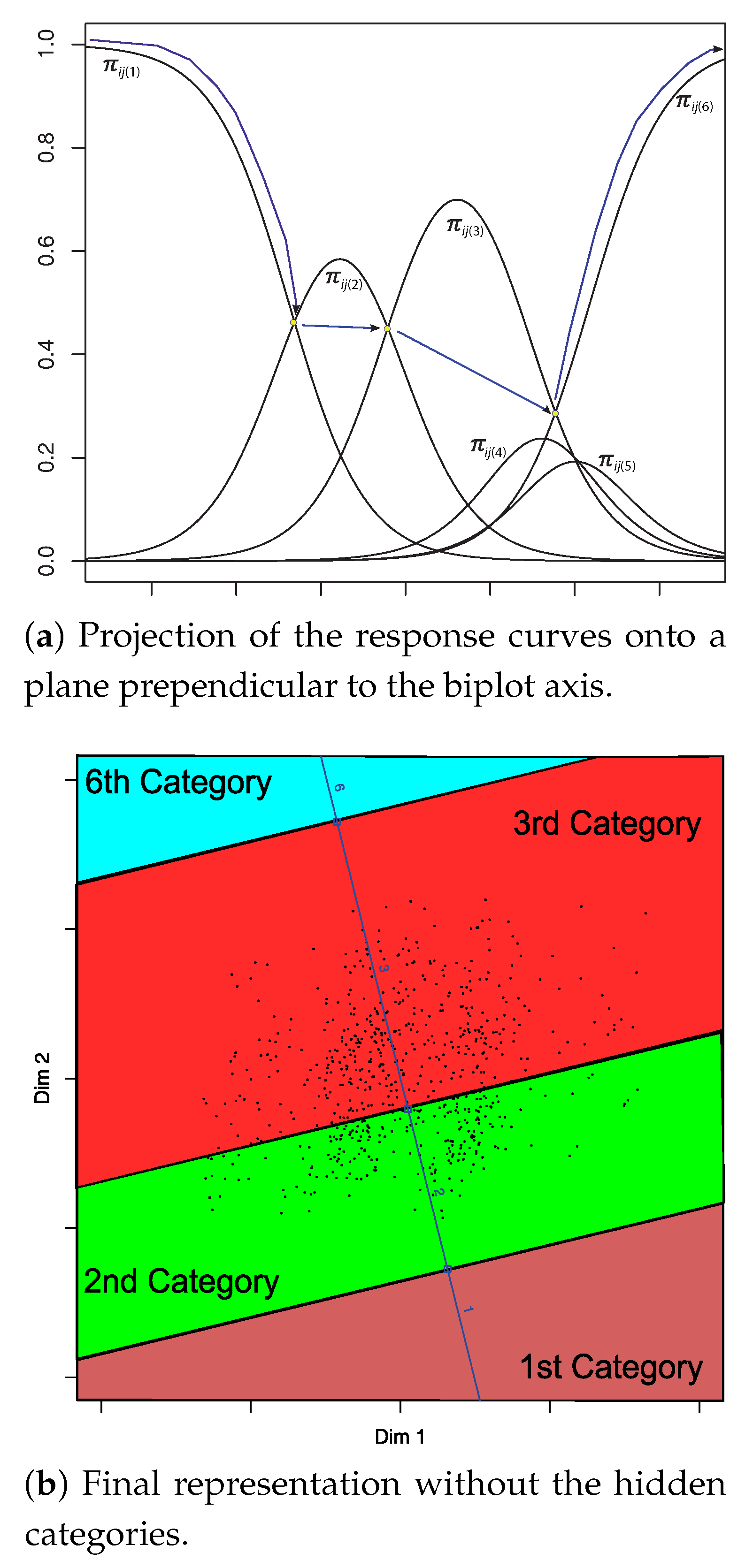
If the row scores where known, obtaining the parameters of the model in 34 is equivalent to fitting a proportional odds model using each item as a response and the row scores as regressors. The response surfaces for such a model are shown in Figure 4. Although the response surfaces are no longer sigmoidal, the level curves are still straight lines, so the set of points on the representation (generated by the columns of ) predicting a particular value for the probability of a category lie on a straight line, and different probabilities for all the categories of a particular variable or item lie on parallel straight lines. A perpendicular to all those lines can be used as "biplot axis" in the sense of [19] and is the direction that better predicts the probabilities of all the categories, that is, projecting any individual point onto that direction, we should obtain an optimal prediction of the category probabilities. As all the categories share the same biplot direction, it would be very difficult to place a different graded scales for each and we will represent just the line segments in which the probability of a category is higher then the probability of the rest. That will result, except for some pathological cases, in as many segments as categories (), separated by points in which the probabilities of two (contiguous) categories are equal. See Figure 5 in which we show the parallel lines representing the points that predict equal probabilities for two contiguous categories and a line, perpendicular to all, that is the "biplot axis". The three parallel lines divide the space spanned by the columns of into four regions, each predicting a particular category of the variable. For a biplot representation we don’t need the whole set of lines but just the "axis" and the points on it, intersecting the boundaries of the prediction regions.
3.2. Obtaining the Biplot Representation
So, if we denote one of those intersection points, it must be on the biplot direction, that is,
and the probability of two, possibly contiguous, categories (for example l and m) at this point, must be equal,
We have omitted index i because probabilities are for a general point and not for a particular individual. Using the condition in 35 we can rewrite the cumulative probabilities (or its ) as
with
Changing the values of z we can obtain the probabilities of each category along the biplot axis. So, finding the point is equivalent to find the values of z in which 36 holds. From those values the original point is obtained solving for x in 38 and then calculating y from 35.
There are some pathological cases in which the probability of one or several categories are never higher than the probability of the rest, in such cases we say that the category is “hidden” or “never predicted” and the number of separating points will be lower than . Those pathological cases have to be taken into account when calculating the intersection points.
Figure 6.
Probability curves for a variable with 6 categories in which two (4 and 5) are hidden or never predicted.
Figure 6.
Probability curves for a variable with 6 categories in which two (4 and 5) are hidden or never predicted.
The existence of abnormal cases means that, not just contiguous, but any pair of categories may have to be compared. Then, many comparisons are possible because the equations are different for each case
- 1-2
- 1-
- 1-
- l-
- l- with
- l-j with
- -
For example, in case (3) 1-, is simple to deduce that
Cases (1), (3), (5) and (7) are simple. In the other 3 combinations we have to solve a quadratic equation to obtain the intersection points. For example, in case (2), the first with the categories, we have to solve , that is
Taking
we have to solve the quadratic equation
with and .
If the roots of the equation are both negative, curves don’t intersect. If it has a positive root, we can calculate the intersection points solving for w and then reversing the transformations to obtain . In a similar way we can calculate the intersection points for cases (4) i- and (6) i-j with .
A procedure to calculate the representation of an ordinal variable on the biplot would be as follows:
- Calculate the biplot axis with equation .
- Calculate the intersection points z and then of the biplot axis with the parallel lines used as boundaries of the prediction regions for each pair of categories, in the following order:
- If the values of z are ordered, there are not hidden categories and the calculations are finished.
-
If the values of z are not ordered we can do the following:
- (a)
- Calculate the z values for all the pairs of curves, and the probabilities for the two categories involved.
- (b)
- Compare each category with the following, the next to represent is the one with the highest probability at the intersection.
- (c)
- If the next category to represent is the process is finished. It not go back to the previous step, starting with the new category.
A simpler numeric procedure could also be developed to avoid the explicit solution of the equations.
- Calculate the predicted category for a set of values for z. For example a sequence from -6 to 6 with small steps (0,01 or 0,01 for example). (The precision of the procedure can be changed with the step)
- Search for the z values in which the prediction changes from one category to another.
- Calculate the mean of the two z values obtained in the previous step and then the values. Those are the points we are searching for.
Hidden categories are the ones with zero frequencies in the predictions obtained by the algorithm.
3.3. Parameter Estimation Based on an Alternated Gradient Descent Algorithm on the Cumulative Probabilities
The alternated algorithm described in [33], can be easily extended replacing binary logistic regressions by ordinal logistic regressions. The problem with this approach is that the parameters for the individuals can not be estimated when the individual has 0 or 1 in all the variables for the binary case, or all the responses are at the baseline category for the ordinal case. There is also some problems when perfect probability predictions are present and then there is a perfect separation of some of the categories. The procedure would be similar to the joint maximum likelihood estimation of Item Response Theory (IRT) models. An algorithm for the cumulative probabilities has been developed in [7]. We propose an alternative algorithm based on an alternated gradient descent procedure and the biplot representation described before.
We use cumulative probabilities together with a recursive procedure similar to the one used for binary (data) based on gradient descent methods.
The cost function based on cumulative probabilities is
where the expected cumulative probabilities are
We will use a recursive procedure as in the binary case, estimating first the thresholds and fixing them the parameters for the dimensions one at a time. That would be equivalent to subtract the mean for continuous data.
The gradients for the binary case are easily generalized to the ordinal case by using the cumulative probabilities. The updates are then
Let and the vectors containing the row and column parameters for dimension s. Let an indicator matrix in which, the column, takes the value 1 for the rows corresponding to categories of the variable, and 0 elsewhere. Then the columns of the matrix
contain for each variable. The updates are written in matrix form
For large data matrices it may be convenient to summarize the data into a matrix (and the corresponding ) containing unique patterns in the data and a vector with the frequencies of each pattern . The equations of the gradient descent method can be written now as:
We can organize the calculations in an alternated algorithm that alternatively calculates parameters for rows and columns for each dimension s fixing the parameters already obtained for each previous dimensions. Before that, the constants have to be fitted separately. The algorithm will produce decreasing values of the cost function and eventually will converge at least to a local minima. A good strategy would be starting at different points and select the solution with lower cost.
The procedure would be as follows:
| Algorithm 2 Algorithm to calculate the Components for Ordinal Data |
|
3.4. Factorization of the Polychoric Correlation Matrix
There is another way of obtaining the parameters: The factorization of the polychoric correlations matrix.
The idea is that the observed categorical responses are discretized versions of a continuous process.
Consider an ordinal variable with categories. This variable is assumed to arise from an underlying continuous variable that follows a standard normal distribution. There are thresholds, , which divide the continuous variable into ordinal categories.
The relationship between and can be expressed as:
The polychoric correlations are the correlations among the . Let a matrix containing the polychoric correlations among the J ordinal variables and let the thresholds.
We can factorize the matrix as
where contains the loadings of a linear factor model for the underlying variables.
It can be shown the there is a close relation between the factor model in 51 and the model in 31. You can find the details in [23].
If the factor model loadings and he thresholds are known, the parameters for the variables in our model (31) can be calculated as:
The remaining parameters for te individuals can then be estimated using the gradient descent method with the cost function in (39) with fixed column parameters and equations (), () or ().
On the other hand, if we have the biplot parameters as in 31, we can obtain the factor model in 51 as:
Then, if we the biplot parameters, we can also interpret the dimensions as in a traditional factor analysis sing factor loadings and communalities.
3.5. Goodness of Fit
The log-likelihood can be used as a measure of the overall goodness of fit, specially for comparison of different models containing, for example, a different number of dimensions. Statistical tests similar to those proposed in the context of IRT models could be used here, in particular, tests based on ordinal logistic regressions. [26] propose tests based on logistic regressions for binary data that could easily be extended to ordinal data. On one hand, the statistical tests for this situations have many problems and on the other hand we see the procedure more as a descriptive exploratory model, so we are less interested in global statistical tests and more in goodness of fit indices or tests for each separate variable. For IRT models, the items are closely related to one or several latent dimensions and all are useful to describe the latent factors, so there must be an adequate overall goodness of fit. In a more general exploratory situation some of the variables may not be useful for describing the problem, inducing a lower overall fit that can lead to miss-interpretations. [8], conduct a simulation study in which some irrelevant variables and noise are added to a known structure, showing that the known structure is recovered even when the overall goodness of fit is not high. Using fit indices for each variable, they are able to identify the relevant and eliminate the irrelevant variables. A similar result can be found in [12].
Several tests and goodness of fit indices can be defined for each variable considering that has been fitted using an ordinal logistic regression with proportional odds. Here we use the likelihood ratio test to compare the model with constant probability (no latent dimensions) with the complete model in exactly the same way as in the standard logistic regression. The test should be interpreted here with care because the latent variables are also estimated inside the procedure and its variation is not considered explicitly in the test; nevertheless is an indication of the significance of the variable to describe the data. For classical linear biplots no such tests are usually performed but goodness of fit indices are calculated. In [18] predictivities as the percentage of the variance of each variable explained by the dimensions, i. e., is a measure of the prediction accuracy on the biplot, is defined. The predictivity is used as a measure of goodness of fit measure by the package BiplotGUI ([24]) In the context of Correspondence Analysis those quantities were called relative contributions of the axis to the elements (variables or individuals) (see [3,20] or [3]) extended to biplots by [15] or [20]. Contributions of the dimensions to the variables can be interpreted as squared correlations between observed variables and dimensions.
From another point of view, the predictivity, is the coefficient of determination for the regressions in 8. For ordinal responses, a pseudo as the Cox-Senell or Nagelkerke can be used.
Another possible measure of goodness of fit is the percentage of correct classifications. We calculate two percentages, one for the cumulative probabilities and another one for the original categories. The observed and predicted items are both ordinal so, for measuring the association between them we use the weighted kappa coefficient.
4. An Empirical Study
4.1. Dataset
In 2008, for a set of 26 countries worldwide, among which was Spain, setting 2006 as reference year and following the guidelines set by the Organization for Cooperation and Development(OECD), the department of statistics of UNESCO and Eurostat (Statistical Office of the European Union), began to do surveys to people that had obtained a PhD degree, and that therefore are doctorates, with the objective of having a clearer information about their characteristics. Most of the pioneer countries belonged the European Union, although members of the OECD, as USA or Australia, also participated. In the Spanish case, it was the National Institute of Statistics (Instituto Nacional de Estadistica - INE) which focused all efforts to carry out this new operation with the objective that the availability of information in this field had continuity in time. Thus, the so-called “Survey on Human Resources in Science and Technology” was established as part of the general plan of science and technology statistics carried out by the European Union Statistics Office (Eurostat). This need for information is evident in the European Regulation 753/2004 on Science and Technology, which specifies the production of statistics on human resources in science and technology.
Surveys on doctorates (CDH: Careers of doctorate holders) try to measure specific demographic aspects related to employment, so that the level of investigation of this group, the professional activity carried out, the satisfaction with their main job, the international mobility and the income of this group can be quantified in Spain.
The study focused on all the doctorate holders resident in Spain, younger than 70, that obtained their degree in a Spanish university, both public or private, between 1990 and 2006. The frame of this statistical operation was a directory of doctorate holders provided to the National Statistic Institute by the University Council, which includes all the persons who have defended a doctoral thesis in any Spanish university, according with their electronic databases, which was comprised of approximately 80000 people. Doctors belong to the level 6 of the international classification of education ISCED-97. This level is reserved for tertiary programs which lead to the award of an advanced research qualification and devoted to advanced study and original research and not based on course-work only.
As for the sampling design, a representative sample was designed for each region at NUTS-2 level. The NUTS classification (Nomenclature of Territorial Units for Statistics) is a hierarchical system for dividing up the economic territory of the EU for different purposes. (see Eurostat) , using a sampling with equal probabilities. The doctors were grouped according to their place of residence, and the selection has been done independently in each region by equal probability with random start systematic sampling. A sample of 17000 doctors was selected. The sample has been distributed between the regions assigning the 50% in an uniform way and the rest proportional to the size of them, measured in number of doctorate holders that have their residence in those regions.
The INE used a questionnaire harmonized at European level, structured in several modules, that can be found at the website of the Institute (INE). As a result of the collection process it was obtained a response rate at the national level of 72%.
We have 12193 doctorate’s answers to the questionnaire in Spain to develop this study. We will focus our attention on the module C (Employment situation) and specifically, in the subsection C.6.4, that tries to find out the level of satisfaction of the doctorate holders in aspects related to their main job. This question has several points of interest coded on a likert scale from 1 to 4 (see Figure 7).
Each item will be considered as ordinal, then we have 11 items or variables in total. For an easier interpretation codification the answers to each question have been inverted in such a way that higher numbers are associated to better satisfaction. Then the final codification is: 1-Very dissatisfied, 2-Somewhat dissatisfied, 3-Somewhat satisfied and 4-Very satisfied.
4.2. Results
Using the alternated algorithm to estimate the parameters of the two-dimensional model, we have obtained the fit indicators in Table 1, the factor loadings and communalities in Table 2 and the explained variances in Table 3.
All the variables fit reasonably well to the model as indicated for the different fit measures. All the are reasonably high. For example, Nagelkerke pseudo values range from 0.36 to 0.65 that would be considered by most authors as reasonably high. The same would apply for the other pseudo- measures.
The percents of correct classifications for he cumulative probabilities are quite high , from 85.40% to 91.65%, with a global percent of 88.03%. For the original ordinal values is smaller, from 56.06% to 71.53%, with a global rate of 64.95%. We have to take into account that we have optimized the cumulative distributions rather than he original ordinal values.
The Kappa coefficients are not very high, probably due to the fact that we have optimized the cumulative distribution rather than the original values. In any case, all the indices are just indicators of what variables fit better to the model, that is, what variables have a higher relation to the latent factors.
Analyzing the interpretation of two dimensions or factors, using their loadings, the first has higher weights for the variables, opportunities for advancement, degree of independence, intellectual challenge, level of responsibility and contribution to society, which are features associated to intellectual satisfaction. The second factor presents higher values for salary, benefits, job security and working conditions, all related with economical and work satisfaction. Then we have two main almost independent factors, the first related to the intellectual aspects and the second to the job conditions. The job location and social status variables have similar loadings in both factors meaning that are related to both. The angle between the variables defining each factor is close to 90°, which means that satisfaction with income and work seems to be nod correlated with intellectual, something that also appears in other European countries, as is evident in the Austrian case [29].
The variance explained by two factors is 65.94% as shown in Table 3.
The biplot of ordinal data can be seen in Figure 8, in which points represent to individuals and the directions to variables. Together with the measures presented before, graphical representations are useful tools for interpreting patterns in data; biplots also can simultaneously find important features in individuals and variables and relations among them.
In general angles between directions are interpreted as correlations like in classical biplots, actually polychoric correlations among ordinal variables in this case. Acute small angles are interpreted as high positive correlation, almost straight angles as high negative correlation and right angles as no correlation.
Some of the variables have a similar behavior, such as level of responsibility, challenge or contribution to society, because angles between its directions are small. Although there are groups of variables whose directions are very similar, the position of the categories are quite different from each other within those groups. This happens with opportunities for advancement and degree of independence.
Markers for individuals are represented by small dots and not labeled because the plot would be too crowded and, in this case, a particular individual is not studied. In general, distances among points representing individuals are related to their similarity. The closer two points are, the more similar. Normally this allows to find clusters of similar individuals and the variables or items responsible for groupings. Cluster may also be defined by external nominal variables to investigate if the factors are related to it.
The projection of an individual into a direction for a variable predicts categories of the variables. The points separating the prediction of the categories ar marked on each direction (variable, item) with numbers. For example, points marked with number 1 are the threshold to change the prediction from the first to the second category, 2 is the threshold from the second to the third an so on.
The figure can be improved using different colors for each variable as in Figure 9. The colors may help identifying marks for each variable.
All the variables have three marks except job security that has 2 (1 and 2) meaning that the category 3 is never predicted or hidden, that is, the probability oh having the second category is never higher than probabilities for other categories.
The plot reflects the factor structure of the data set in a graphical way. To illustrate how the representation gets the structure of a particular variable we can add to the plot clusters with points with different observed categories. Figure 10 such a representation for variable Chalenge
We notice that the cluster centers are arranged nearly along the direction of Challenge, indicating that this axis effectively reflects the behavior of that variable. A similar analysis can be carried out for the other variables, confirming that the plots capture information from all of them, though to varying degrees. The fit measures provide an indication of how well each variable is represented.
The final plot can be also used to check the behavior of different groups of individuals defined by external nominal variables, for example, males and females to investigate the relation between satisfaction and sex. Figure 11.
The positions of men and women, measured as centroids of coordinates on the biplot for each group, are virtually indistinguishable (Figure 11), meaning that there is a very small difference between men and women in the way they perceive satisfaction with doctorate degrees.
5. Software Note
Author Contributions
All authors have read and agreed to the published version of the manuscript and contributed equally to the paper.”
Funding
This research received no external funding.
Informed Consent Statement
Not applicable.
Data Availability Statement
Data is publicly available at he web of the Instituto navional de Estadística de España (INE),
Conflicts of Interest
The authors declare no conflicts of interest.
References
- Babativa-Márquez, J. G. and Vicente-Villardón, J. L. Logistic biplot by conjugate gradient algorithms and iterated svd. Mathematics 2015, 9, 2015.
- Baker, F. (1992). Item Response Theory. Parameter Estimation Techniques. Marcel Dekker.
- Benzecri, J. P. (1976). L’analyse des donnees. Dunod.
- Canal, J. F. and Muniz, M. A. Professional doctorates and the careers: Present and future. the spanish case. European journal of education. 2012, 47, 153–171. [CrossRef]
- Cañueto, J., Cardeñoso-Álvarez, E., García-Hernández, J., Galindo-Villardón, P., Vicente-Galindo, P., Vicente-Villardón, J., Alonso-López, D., De Las Rivas, J., Valero, J., Moyano-Sanz, E., et al. (2017). Micro rna (mir)-203 and mir-205 expression patterns identify subgroups of prognosis in cutaneous squamous cell carcinoma. British Journal of Dermatology, 177(1):168–178.
- de Leeuw, J. (2006). Principal component analysis of binary data by iterated singular value decomposition. Computational Statistics and Data Analysis, 50(1):21–39.
- de Rooij, M., Breemer, L., Woestenburg, D., and Busing, F. (2024). Logistic multidimensional data analysis for ordinal response variables using a cumulative link function. Psychometrika, pages 1–37.
- Demey, J., Vicente-Villardón, J. L., Galindo, M. P., and Zambrano, A. (2008). Identifying molecular markers associated with classification of genotypes using external logistic biplots. Bioinformatics, 24(24):2832–2838.
- Gabriel, K. (1971). The biplot graphic display of matrices with application to principal component analysis. Biometrika, 58(3):453–467.
- Gabriel, K. R. (1980). Biplot display of multivariate matrices for inspection of data and diagnosis. Technical report, ROCHESTER UNIV NY.
- Gabriel, K. R. (1998). Generalised bilinear regresion. Biometrika, 85(3):689–700.
- Gabriel, K. R. (2002). Goodness of fit of biplots and correspondence analysis. Biometrika, 89(2):423–436.
- Gabriel, K. R., Galindo, M. P., and Vicente-Villardon, J. L. (1998). Use of Biplots to diagnose independence models in contingency tables., pages 391–404. Academic Press.
- Gabriel, K. R. and Zamir, S. (1979). Lower rank approximation of matrices by least squares with any choice of weights. Technometrics, 21(4):489–498.
- Galindo-Villardon, M. P. (1986). Una alternativa de representacion simultanea: Hj-biplot. Questiio, 10(1):13–23.
- Gallego, I. and Vicente-Villardon, J. L. (2012). Analysis of environmental indicators in international companies by applying the logistic biplot. Ecological Indicators, 23(0):250 – 261.
- Gallego-Alvarez, I., Ortas, E., Vicente-Villardón, J. L., and Álvarez Etxeberria, I. (2017). Institutional constraints, stakeholder pressure and corporate environmental reporting policies. Business Strategy and the Environment, 26(6):807–825.
- Gardner-Lubbe, S., Le Roux, N., and Gower, J. (2008). Measures of fit in principal component and canonical variate analyses. Journal of Applied Statistics, 35(9):947–965.
- Gower, J. and Hand, D. (1996). Biplots. Monographs on statistics and applied probability. 54. London: Chapman and Hall., 277 pp.
- Greenacre, M. J. (1984). Theory and Applications of Correspondence Analysis. Academic Press.
- Hernández, J. C. and Vicente-Villardón, J. L. (2013). Ordinal Logistic Biplot: Biplot representations of ordinal variables. Universidad de Salamanca.Department of Statistics. R package version 0.3.
- Hernández-Sánchez, J. C. and Vicente-Villardón, J. L. (2017). Logistic biplot for nominal data. Advances in Data Analysis and Classification, 11(2):307–326.
- Jöreskog, K. G. and Moustaki, I. (2001). Factor analysis of ordinal variables: A comparison of three approaches. Multivariate Behavioral Research,, 36(3):347–387.
- la Grange, A., le Roux, N., and Gardner-Lubbe, S. (2009). Biplotgui: Interactive biplots in r. Journal of Statistical Software, 30(12).
- Lee, S., Huand, J., and Hu, J. (2010). Sparse logistic principal component analysis for binary data. Annals of Applied Statistics, 4(3):21–39.
- Mair, P., Reise, S. P., and Bentler, P. (2008). Irt goodness-of-fit using approaches from logistic regression. UCLA Statistics Preprint Series, 540.
- R Core Team (2021). R: A Language and Environment for Statistical Computing. R Foundation for Statistical Computing, Vienna, Austria.
- Samejima, F. (1969). Estimation of latent ability using a response pattern of graded scores. Psychometric Monograph Supplement, 4(34).
- Schwabe, M. (2011). The careers paths of doctoral graduates in austria. European Journal of Education., 46(1):153–168.
- Song, Y., Westerhuis, J. A., and Smilde, A. K. (2020). Logistic principal component analysis via non-convex singular value thresholding. Chemometrics and Intelligent Laboratory Systems, 204:104089.
- Vicente-Galindo, P., de Noronha Vaz, T., and Nijkamp, P. (2011). Institutional capacity to dynamically innovate: An application to the portuguese case. Technological Forecasting and Social Change, 78(1):3 – 12.
- Vicente-Gonzalez, L. and Vicente-Villardon, J. L. Partial least squares regression for binary responses and its associated biplot representation. Mathematics 2022, 10, 2580. [CrossRef]
- Vicente-Villardon, J., Galindo, M., and Blazquez-Zaballos, A. (2006). Logistic Biplots., pages 503–521. Chapman and Hall.
- Vicente-Villardon, J. L. (2022). MultBiplotR: Multivariate Analysis Using Biplots in R. R package version 2.1.3.
- Vicente-Villardon, J. L. and Sanchez, J. C. H. (2014). Logistic biplots for ordinal data with an application to job satisfaction of doctorate degree holders in spain.
Figure 1.
Typical PCA-Biplot with scales for the variables.
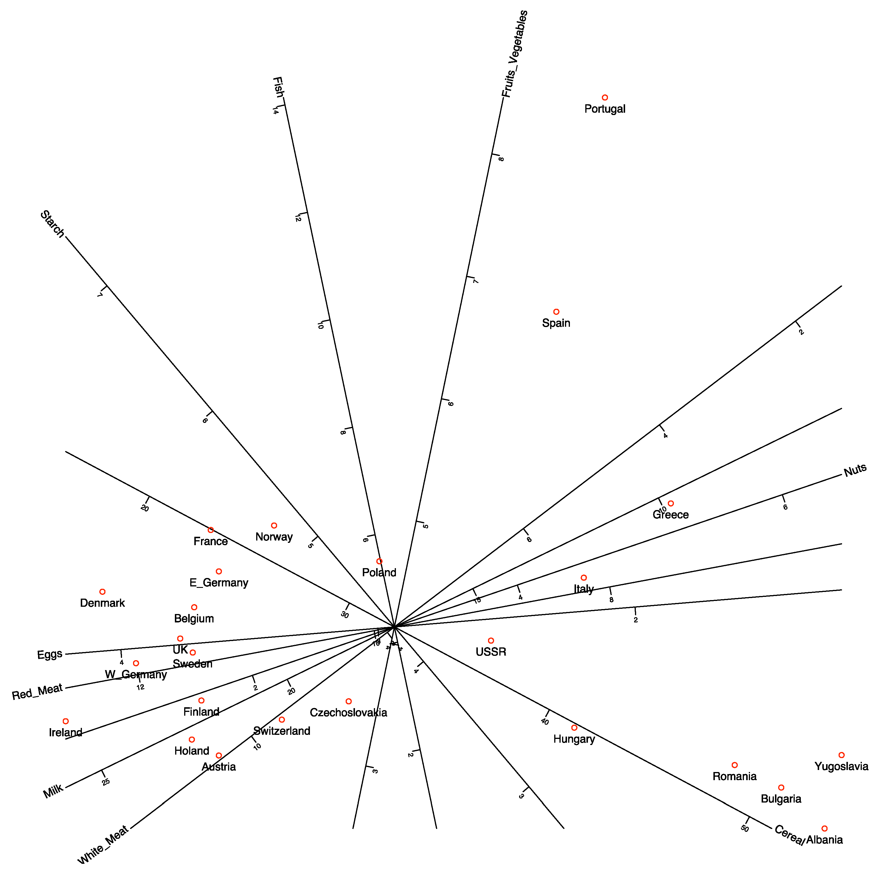
Figure 2.
Typical Binary logistic biplot with probability scales for the variables.
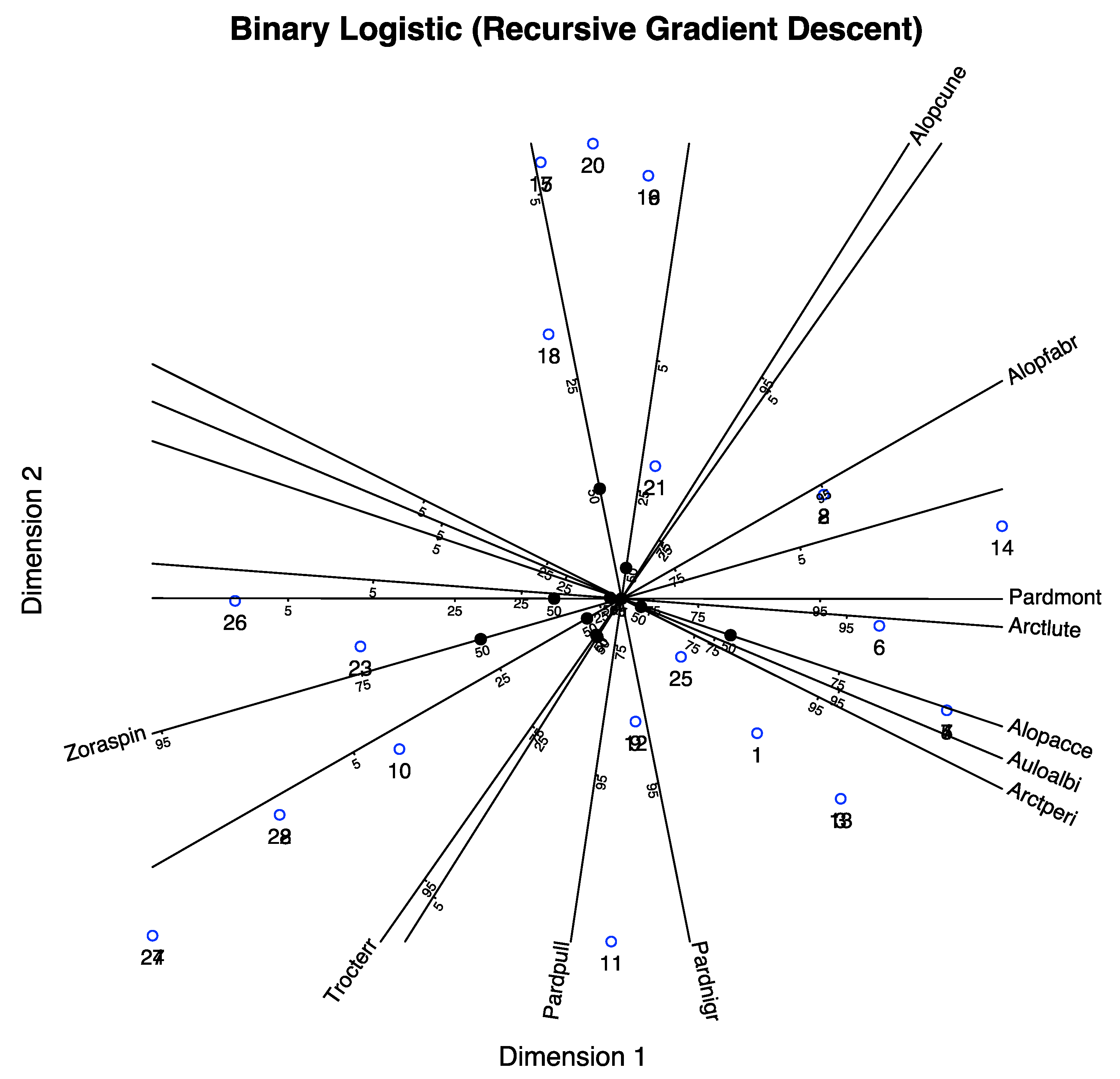
Figure 3.
Cumulative response curves for a two-dimensional latent trait and a variable with four categories.
Figure 3.
Cumulative response curves for a two-dimensional latent trait and a variable with four categories.
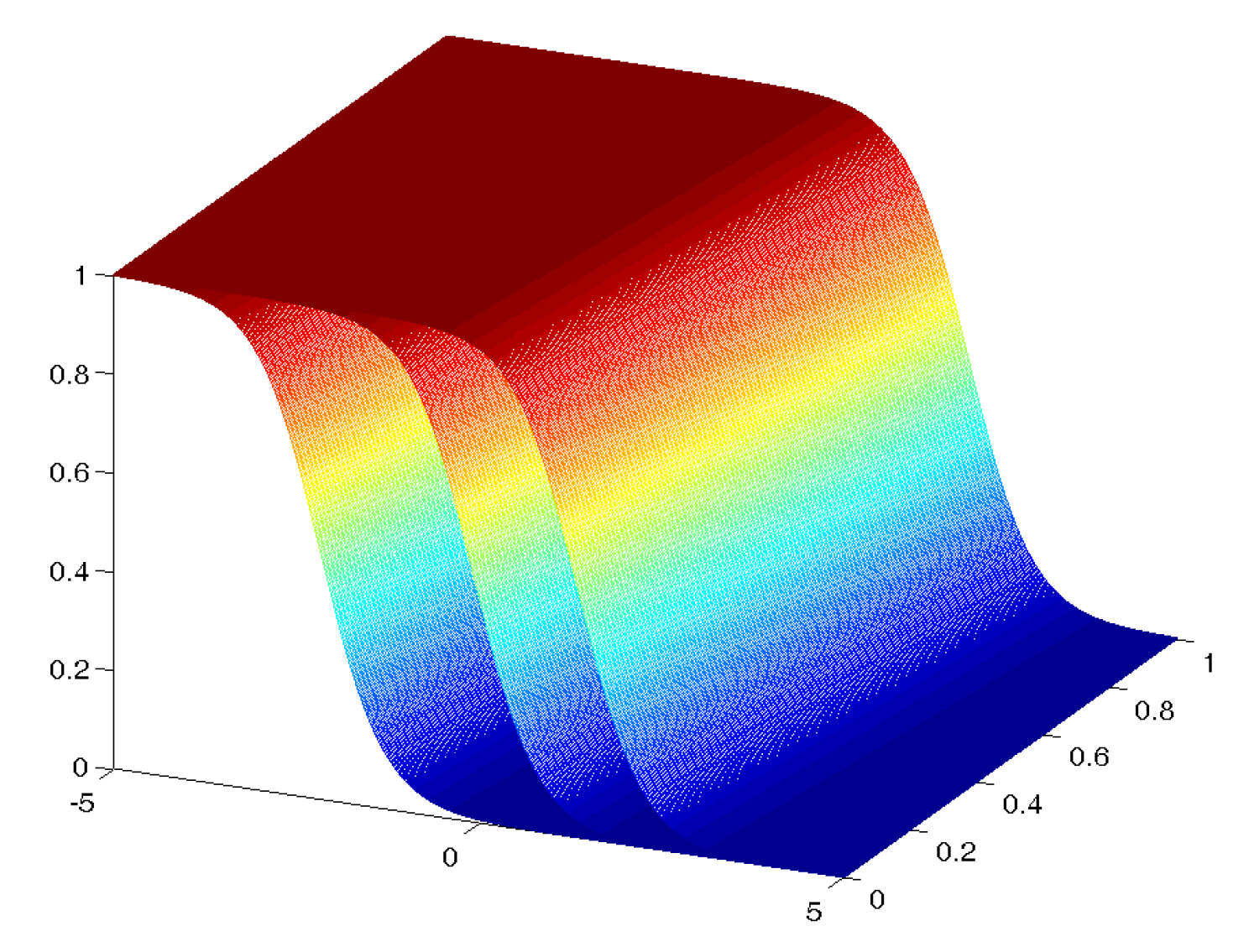
Figure 4.
Response curves for an ordinal variable with four ordered categories.
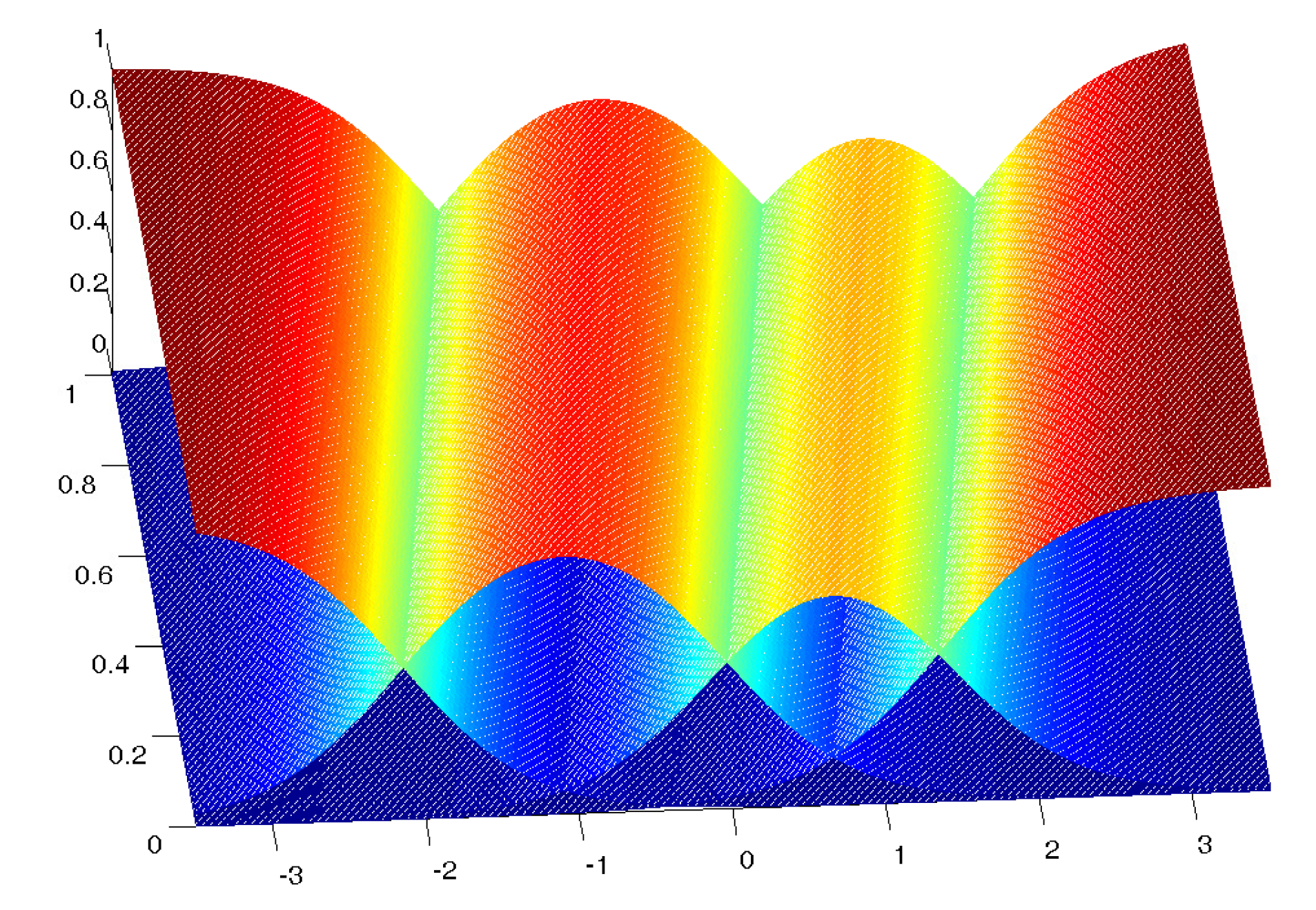
Figure 5.
Prediction regions determined by three parallel straight lines for an ordinal variable with four categories.
Figure 5.
Prediction regions determined by three parallel straight lines for an ordinal variable with four categories.
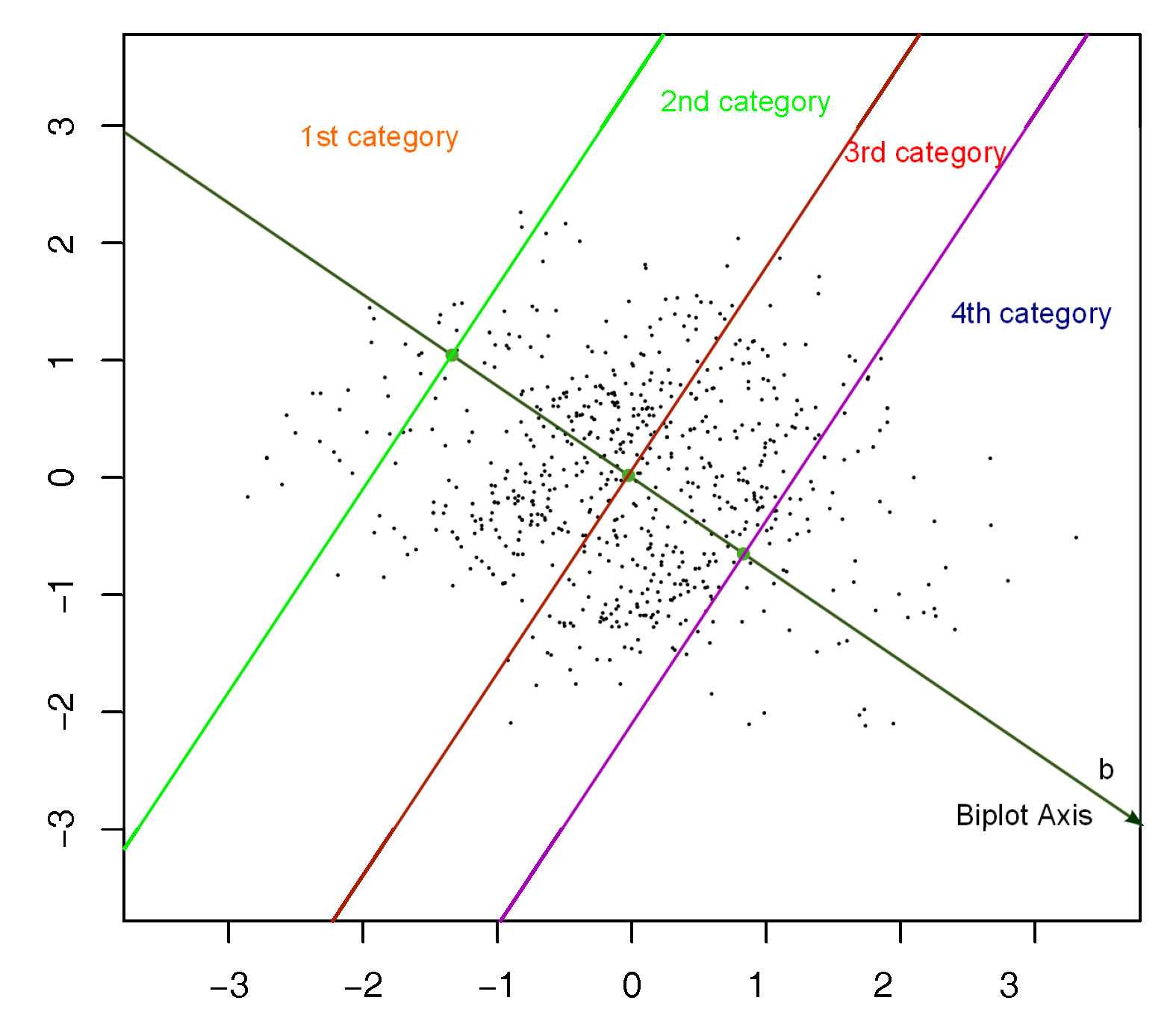
Figure 7.
Question C.6.4 of the questionnaire.

Figure 8.
Ordinal logistic biplot for the satisfaction of the doctorate holders with their principal job in Spain. The labeled marks on each direction are the thresholds for the separation of the prediction among categories.
Figure 8.
Ordinal logistic biplot for the satisfaction of the doctorate holders with their principal job in Spain. The labeled marks on each direction are the thresholds for the separation of the prediction among categories.
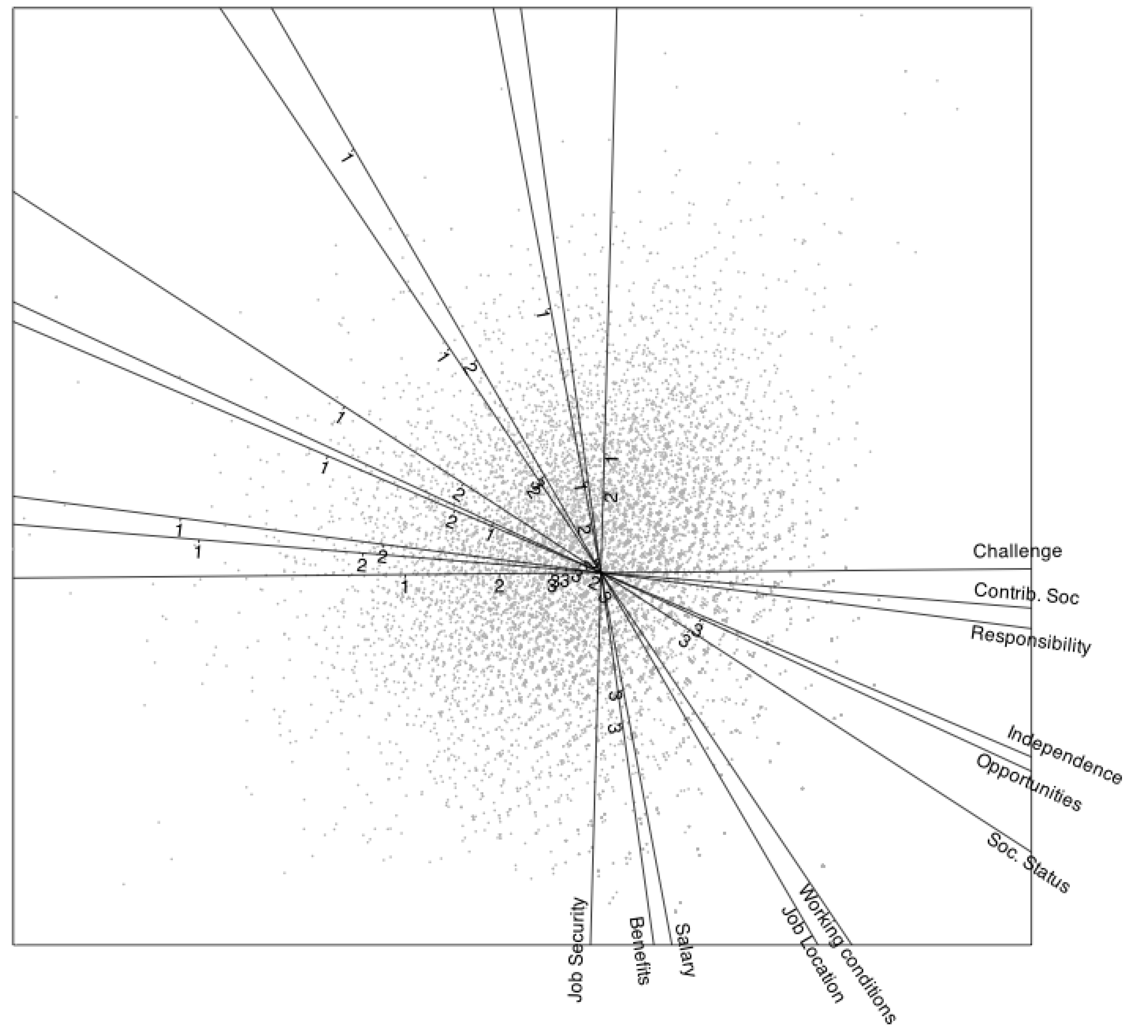
Figure 9.
Ordinal logistic biplot for the satisfaction of the doctorate holders with their principal job in Spain with colored variables.
Figure 9.
Ordinal logistic biplot for the satisfaction of the doctorate holders with their principal job in Spain with colored variables.
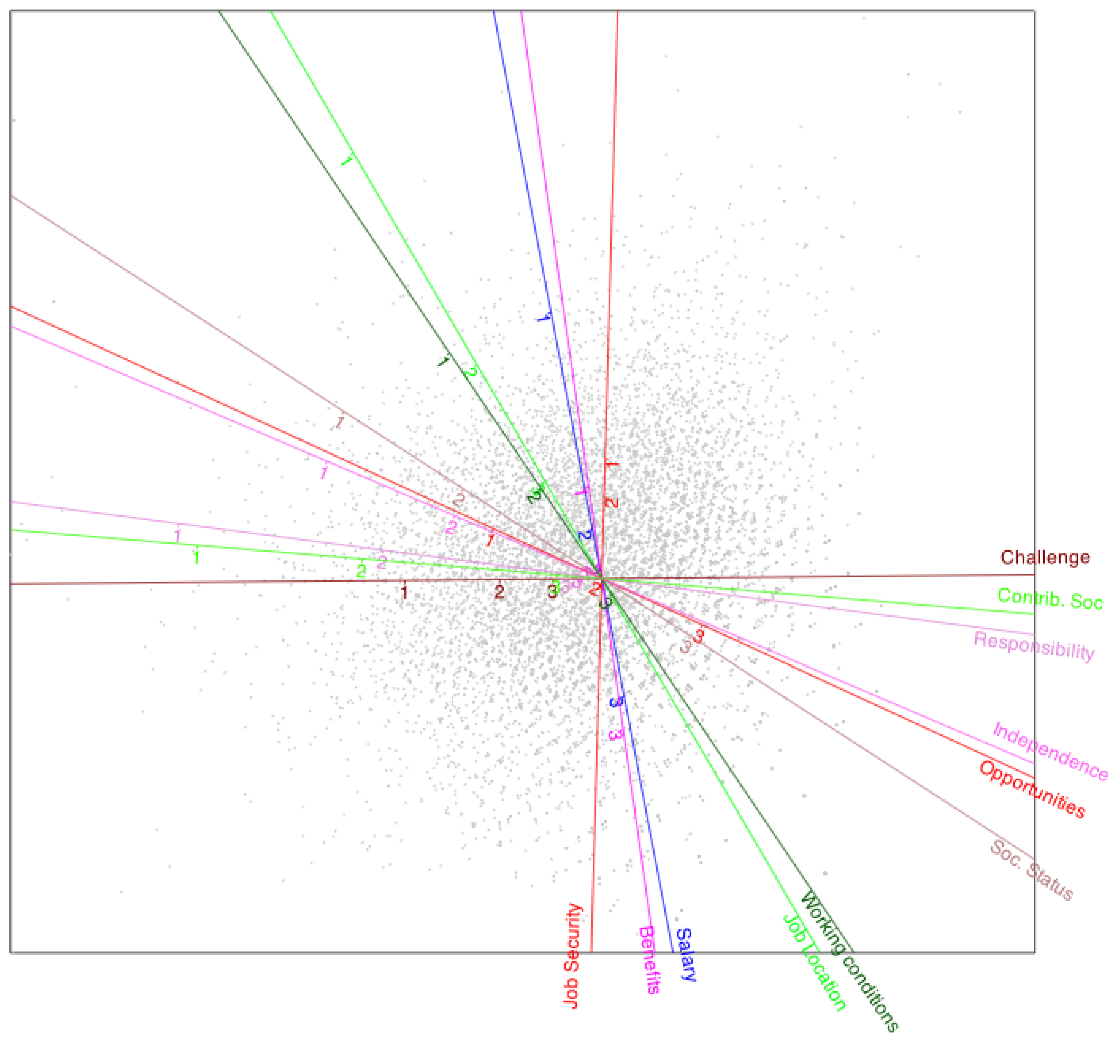
Figure 10.
The points for individuals in each observed categories are covered by a convex hulls in different colors. The centers of clusters are also marked.
Figure 10.
The points for individuals in each observed categories are covered by a convex hulls in different colors. The centers of clusters are also marked.
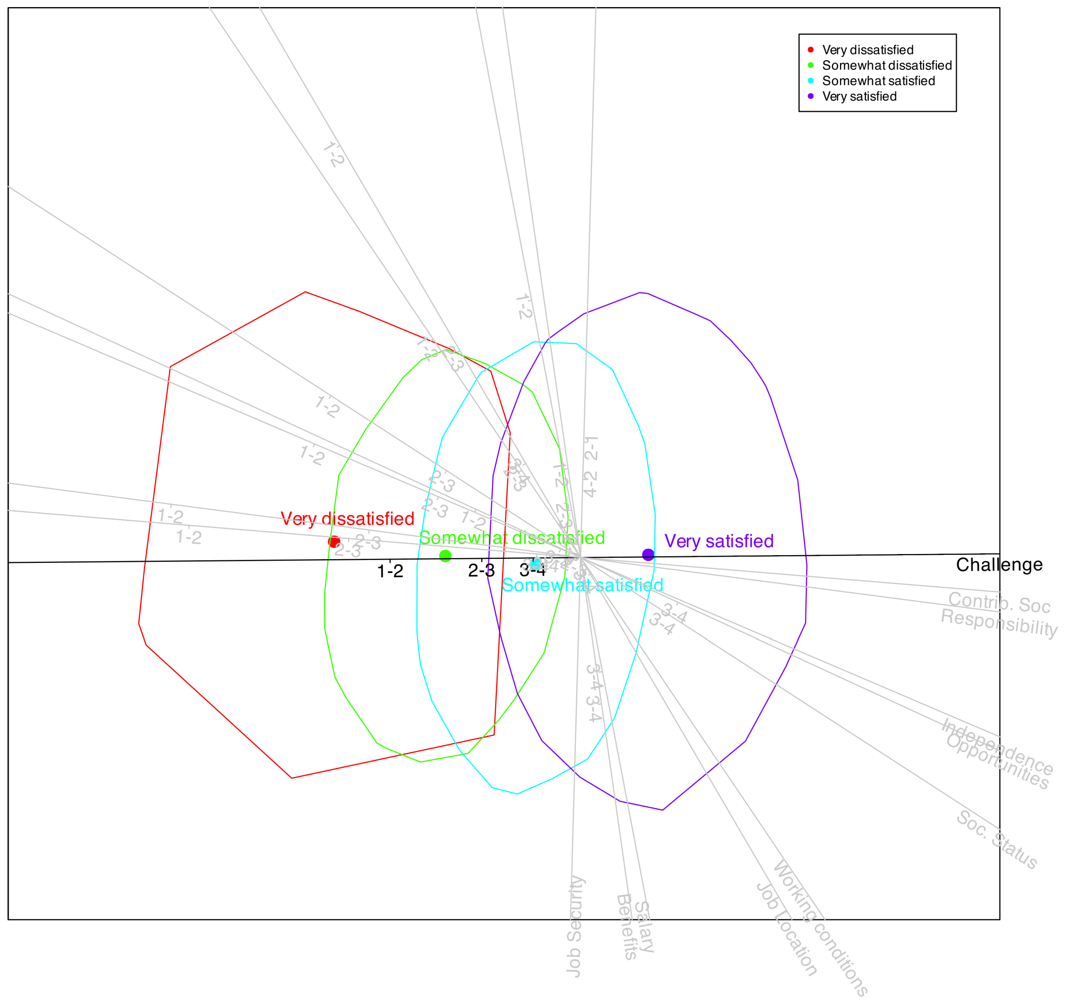
Figure 11.
Ordinal logistic biplot for the satisfaction of the doctorate holders with clusters for each sex.
Figure 11.
Ordinal logistic biplot for the satisfaction of the doctorate holders with clusters for each sex.
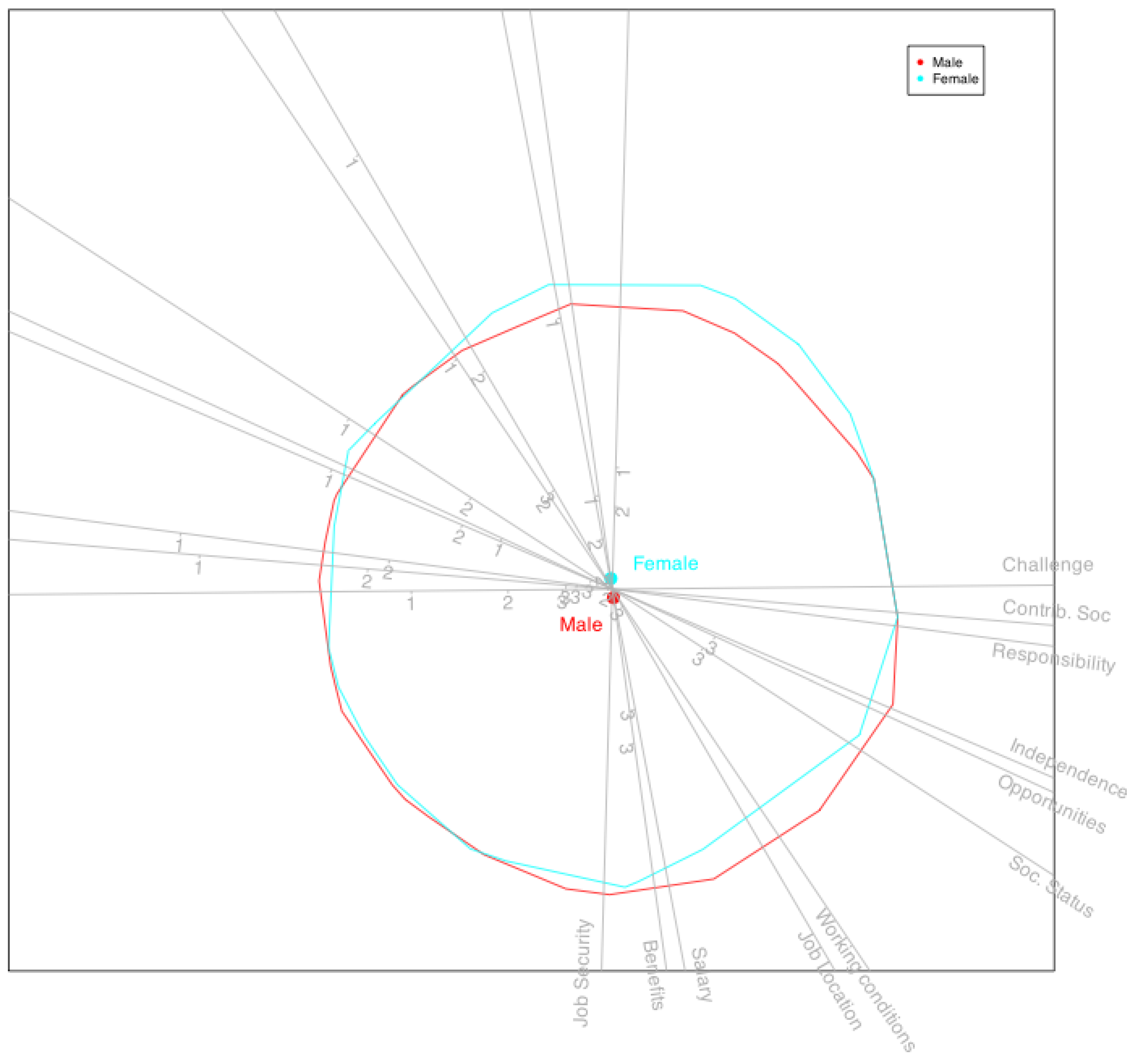

Table 1.
Measures of fit (Global and for each separate variable): PCC(Cum) - Percent of correct classification for the cumulative probabilities; Cox-Snell, MacFadden and Nagelkeke pseudo values; PCC - Percentage of correct classification for the initial values and Kappa coefficient among the observed and expected values.
| PCC(Cum) | Cox-Snell | MacFadden | Nagelkerke | PCC | Kappa | |
|---|---|---|---|---|---|---|
| Salary | 90.49 | 0.53 | 0.67 | 0.53 | 71.26 | 0.58 |
| Benefits | 86.60 | 0.59 | 0.69 | 0.59 | 58.75 | 0.52 |
| Job Security | 86.81 | 0.65 | 0.64 | 0.65 | 65.32 | |
| Job Location | 84.93 | 0.22 | 0.89 | 0.22 | 61.56 | 0.18 |
| Working conditions | 88.81 | 0.53 | 0.69 | 0.53 | 66.04 | 0.55 |
| Opportunities | 85.40 | 0.58 | 0.71 | 0.58 | 56.06 | 0.51 |
| Challenge | 91.65 | 0.65 | 0.58 | 0.65 | 71.53 | 0.64 |
| Responsibility | 87.70 | 0.36 | 0.78 | 0.36 | 63.80 | 0.38 |
| Independence | 87.56 | 0.45 | 0.74 | 0.45 | 63.24 | 0.45 |
| Contrib. Soc | 88.61 | 0.37 | 0.77 | 0.37 | 66.57 | 0.39 |
| Soc. Status | 89.74 | 0.40 | 0.76 | 0.40 | 70.30 | 0.41 |
| Global | 88.03 | 64.95 |
Table 2.
Factor Structure (Loadings and Communalities).
| Dimension 1 | Dimension 2 | Communalities | |
|---|---|---|---|
| Salary | 0.16 | -0.82 | 0.70 |
| Benefits | 0.12 | -0.82 | 0.69 |
| Job Security | -0.02 | -0.86 | 0.74 |
| Job Location | 0.33 | -0.57 | 0.44 |
| Working conditions | 0.47 | -0.70 | 0.72 |
| Opportunities | 0.76 | -0.35 | 0.69 |
| Challenge | 0.87 | 0.01 | 0.76 |
| Responsibility | 0.77 | -0.10 | 0.61 |
| Independence | 0.75 | -0.32 | 0.66 |
| Contrib. Soc | 0.78 | -0.06 | 0.62 |
| Soc. Status | 0.66 | -0.43 | 0.63 |
Table 3.
Variance explained by the Factor Structure.
| Dimension 1 | Dimension 2 | |
|---|---|---|
| Variance | 3.92 | 3.34 |
| Cummulative | 3.92 | 7.25 |
| Percentage | 35.61 | 30.32 |
| Cum. Percentage | 35.61 | 65.94 |
Disclaimer/Publisher’s Note: The statements, opinions and data contained in all publications are solely those of the individual author(s) and contributor(s) and not of MDPI and/or the editor(s). MDPI and/or the editor(s) disclaim responsibility for any injury to people or property resulting from any ideas, methods, instructions or products referred to in the content. |
© 2025 by the authors. Licensee MDPI, Basel, Switzerland. This article is an open access article distributed under the terms and conditions of the Creative Commons Attribution (CC BY) license (http://creativecommons.org/licenses/by/4.0/).
Copyright: This open access article is published under a Creative Commons CC BY 4.0 license, which permit the free download, distribution, and reuse, provided that the author and preprint are cited in any reuse.


