Submitted:
19 August 2025
Posted:
25 August 2025
You are already at the latest version
Abstract
This study investigated the effect of the number of sensors (8, 12, 16, and 20) on the measurement results of stress wave velocity in two-dimensional acoustic tomography of Hoop pine (Araucaria cunninghamii Sweet) trees, and evaluated the method’s accuracy and operational efficiency in tree health diagnostics. Tests were conducted on five sample trees, two of which were confirmed to have internal damage using the drilling resistance method. The results indicated that increasing the number of sensors improved image resolution and information completeness. However, differences in average stress wave velocities among sensor configurations were not statistically significant (p ≥ 0.05), indicating limited variation overall. In healthy trees, stress wave velocities measured under different sensor quantities (e.g., 8 vs. 20) exhibited weak linear correlations (R2 = 0.06–0.58), reflecting relatively uniform internal structures. In contrast, damaged trees showed strong consistency in velocity results (R2 = 0.82–0.91, p < 0.01), and both minimum and average velocities were significantly lower than in healthy trees. These findings demonstrate that acoustic tomography can effectively identify internal tree defects. Even with only eight sensors, decay and cavities can still be accurately detected, enhancing field inspection efficiency and reducing costs, thus showing strong potential for practical applications.
Keywords:
number of sensors
; acoustic tomography
; stress wave velocity
; tree health diagnosis
; minimally invasive technique
; hoop pine (Araucaria cunninghamii Sweet)
1. Introduction
Tree risk assessment aims to evaluate the structural stability of trees and serves as a critical foundation for subsequent management decisions. A widely used approach in such assessments is Visual Tree Assessment (VTA), which involves systematic evaluations based on observable external symptoms (Linhares et al. 2021; Nocetti and Brunetti 2024 [1,2]). However, the internal condition of a tree often cannot be reliably inferred from its outward appearance alone, necessitating the use of Non-Destructive Testing (NDT) or Minimally Invasive Technologies (MIT) to overcome the limitations of VTA and to provide more detailed structural insights. These advanced diagnostic methods have thus become essential tools in comprehensive tree risk evaluation.
Among the available advanced techniques, acoustic tomography and resistance drilling have been widely adopted for assessing internal tree structures with minimal damage (Lin et al. 2025a, b [3,4]). Acoustic tomography works by transmitting stress waves through the tree trunk to detect internal decay and cavities, reconstructing a visualized two-dimensional cross-sectional image (Ishaq et al. 2014 [5]). This technique has proven effective for diagnosing decay in urban trees (Son et al. 2021 [6]), although its image accuracy may still be influenced by multiple factors. In contrast, resistance drilling—while invasive—is considered only minimally so due to its design, and it provides continuous resistance data that can aid in interpreting acoustic images and understanding internal wood structure (Downes et al. 2018; Fundova et al. 2018; Sharapov et al. 2018, 2020 [7,8,9]). When used together, these two techniques offer a more holistic understanding of tree health and contribute to enhancing safety in both urban and rural environments.
This study aims to investigate the impact of sensor quantity on the distribution of stress wave velocity (V) in 2D acoustic tomography images. The specific objectives are to: (1) analyze image differences across various sensor quantities; (2) assess the spatial distribution and variability of V values; (3) examine correlations of V values between different sensor configurations; and (4) compare V values between healthy and damaged regions. The findings are expected to provide a valuable reference for interpreting acoustic tomography images and for assessing the extent of internal trunk damage in practical applications.
In the application of two-dimensional acoustic tomography, the number of sensors (transducers) plays a crucial role in determining image quality and diagnostic reliability. If varying sensor quantities affect stress wave velocity (V) measurements, this can directly influence image interpretation and subsequent assessments. In field practice, especially when inspecting large-diameter trees, limitations in time and labor often restrict the number of sensors that can be deployed. Thus, whether increasing the number of sensors enhances image accuracy and interpretability is a question of both scientific and practical importance. This study explores whether different numbers of sensors result in significant variations in the acoustic images of the same trunk cross-section and whether these variations affect the spatial distribution and variability of stress wave velocity values.
Previous studies have suggested that increasing sensor quantity can enhance image resolution and diagnostic performance. Most existing research has used between 8 and 12 sensors for detecting internal decay and cavities, with a focus on evaluating image accuracy (Gilbert and Smiley 2004; Wang et al. 2009; Ostrovsky et al. 2017 [10,11,12]). Other studies have examined how sensor placement and number influence acoustic imaging outcomes (Liang and Fu 2014; Divos and Divos 2005 [13,14]). However, research remains limited on how sensor quantity affects the numerical variation, spatial distribution, and inter-configuration correlation of stress wave velocity values, particularly in distinguishing between healthy and decayed regions. For example, a study comparing 12 and 24 sensors found that the velocity threshold values used for detecting decay varied depending on the number of sensors employed (Espinosa et al. 2016 [15]). If both acoustic images and stress wave velocities are influenced by sensor quantity, it may be necessary to dynamically adjust the threshold values used for damage detection.
Therefore, this study aims to investigate the impact of sensor quantity on the distribution of stress wave velocity (V) in 2D acoustic tomography images. The specific objectives are to: (1) analyze image differences across various sensor quantities; (2) assess the spatial distribution and variability of V values; (3) examine correlations of V values between different sensor configurations; and (4) compare V values between healthy and damaged regions. The findings are expected to provide a valuable reference for interpreting acoustic tomography images and for assessing the extent of internal trunk damage in practical applications.
2. Materials and Methods
2.1. Experimental Materials
This study was conducted at the Gongguan Campus of National Taiwan Normal University, located in the Wenshan District of Taipei City, Taiwan. Hoop pine (Araucaria cunninghamii Sweet) trees growing along the roadside were selected as the research subjects. To ensure effective detection of the internal condition of tree trunks, sample trees with a diameter at breast height (DBH) greater than 70 cm were chosen for analysis. A total of five qualified trees were selected for subsequent acoustic tomography and resistance drilling tests.
This study was conducted at the Gongguan Campus of National Taiwan Normal University, located in the Wenshan District of Taipei City, Taiwan. Hoop pine (Araucaria cunninghamii Sweet) trees were examined during the period of March 2025. Trees growing along the roadside were selected as the research subjects. To ensure effective detection of the internal condition of tree trunks, sample trees with a diameter at breast height (DBH) greater than 70 cm were chosen for analysis. The estimated age of the sampled trees, based on visible annual growth rings, is between 47 and 51 years, determined using an increment corer to extract core samples. A total of five qualified trees were selected for subsequent acoustic tomography and resistance drilling tests.
2.2. Experimental Methods
This study aimed to investigate the effect of different numbers of sensors on the two-dimensional (2D) acoustic tomographic imaging of stress wave velocity in the trunks of Araucaria cunninghamii. Resistance drilling was also employed to assist in evaluating the internal wood condition. The experimental procedure consisted of two major parts: acoustic tomography and resistance drilling tests.
2.3. Acoustic Tomography
A Fakopp 3D Acoustic Tomograph (Fakopp Enterprise Ltd., Sopron, Hungary; version 6.5 [Fakopp 2020 [16]]) was used to perform acoustic scanning on the five sample trees to construct 2D images of stress wave velocity across trunk cross-sections. The equipment was operated and the software used in accordance with the user manual (Michael et al. 2021 [17]). The system measured the transmission time and velocity of stress waves along various paths across the tree trunk cross-section to obtain raw data for image reconstruction.
During testing, sensors were evenly distributed around the trunk in a horizontal plane at a height of 30 cm above ground. Each sample tree was scanned using 8, 12, 16, and 20 sensors, respectively. ArborSonic 3D software (v5.3.164; Fakopp Enterprise Ltd.) was used to generate the tomographic images. Stress wave data were collected by repeatedly tapping each sensor to ensure a complete data matrix. The generated stress wave frequency ranged between 35 and 40 kHz. This method of generating mechanical stress waves helped improve the consistency and reliability of data collection for subsequent analysis. The software automatically calculated stress wave velocities and produced 2D tomographic images showing lateral distributions of wave speeds. The acoustic tomography procedure is illustrated in Figure 1.
2.4. Resistance Drilling Test
To further assess the internal wood condition of the sample trees and validate the acoustic tomographic interpretations regarding regions of differing wave velocities, resistance drilling tests were conducted on the five Araucaria cunninghamii trees with no apparent external defects. A RESI PD500 resistance drill (IML, Kennesaw, Georgia, USA) was used for the testing.
On the cross-section of each tree, radial drillings were conducted in four directions—east, south, west, and north—extending from the bark toward the center. During the drilling process, the device recorded variations in drilling resistance, producing resistance amplitude profiles. The drill bit specifications were as follows: The drill bit specifications were as follows: a cylindrical drill bit with a tip diameter of 3.0 mm, a shaft diameter of 1.5 mm, and made of stainless steel with a special coating. The drill bit features a sharp conical tip designed for efficient penetration.
The RESI PD500 had a maximum drilling depth of 500 mm and a resolution of 0.1 mm, providing data on drilling depth with a 1:1 scale to ensure measurement accuracy. The test parameters were set as follows: one resistance amplitude value was recorded every 0.1 mm, the feed rate was 100 cm/min, and the drill rotation speed was 2500 RPM. The resulting profiles were used to assess wood soundness and identify potential decay or hollow zones, serving as a reference for interpreting the acoustic tomography images.
3. Results
3.1. Drilling Resistance Amplitude Analysis
This study employed a minimally invasive resistance drilling technique to evaluate the internal wood structure of tree trunks by analyzing the amplitude variation curves recorded during drilling. This technique allowed the spatial identification of both sound and defective regions and served as a reference for subsequent comparisons with stress wave velocity images generated under different sensor configurations. Five sample trees were tested, with radial drillings conducted in four directions (north, south, east, and west) on each tree. Each drilling path extended from the bark to the central axis, and resistance amplitude data were recorded throughout the process (Figure 2).
The measured data showed that sound wood generally exhibited higher drilling resistance amplitudes compared to areas with structural defects, such as decay or cavities. A threshold was set at 70% of the amplitude value for sound wood. Based on this criterion, the results indicated that Tree No. 4 and Tree No. 5 exhibited localized amplitude values below the threshold, confirming the presence of internal defects. Specifically, Tree No. 4 had a defective area concentrated on the northern cross-section, covering 13.3% (damage area) of the total area and showing an asymmetrical distribution. Tree No. 5 exhibited defects near the central axis, occupying 9.4% of the cross-sectional area.
In contrast, the average amplitudes in all four directions of the sound trees (Tree No. 1, 2, and 3) ranged from 16.9% to 27.1%, significantly higher than the 4.1%–19.2% range observed in the defective trees. These ranges did not overlap, indicating that the selected threshold effectively distinguished structural integrity differences.
In the subsequent analytical stage, the damaged areas identified through resistance drilling were used as fixed references for grid-based numerical analysis of the stress wave velocity images. This approach verified the effect of different sensor numbers on the accuracy of interpreting two-dimensional tomographic images, while minimizing bias from subjective interpretation. Notably, the applicability of the amplitude threshold may be influenced by species-specific properties and environmental factors (e.g., wood moisture content). Future research is recommended to incorporate species-specific calibration models and integrate high-resolution tomographic imaging technologies to enhance the accuracy of defect volume estimation.

Table 1.
Average drilling amplitude at four orientations (N, W, S, E) in sampled trees (Unit: %).
| Position | N | W | S | E | WN | EN |
|---|---|---|---|---|---|---|
| No.1 | ||||||
| Average | 20.3 | 16.9 | 19.9 | 19.5 | X | X |
| SD | 3.4 | 2.3 | 3.5 | 2.7 | ||
| No.2 | ||||||
| Average | 16.9 | 17.9 | 18.8 | 27.1 | X | X |
| SD | 7.9 | 2.9 | 3.1 | 12.5 | ||
| No.3 | ||||||
| Average | 21.0 | 23.1 | 22.5 | 20.1 | X | X |
| SD | 4.0 | 4.9 | 4.4 | 3.6 | ||
| No.4 | ||||||
| Average | 6.4 | 16.3 | 19.2 | 16.6 | 4.1 | 18.0 |
| SD | 7.3 | 4.1 | 1.8 | 3.3 | 6.5 | 4.1 |
| No.5 | ||||||
| Average | 16.9 | 17.9 | 17.8 | 21.3 | X | X |
| SD | 6.6 | 5.7 | 5.4 | 10.0 | ||
3.2. Stress Wave Velocity 2D Tomographic Image Analysis
According to Table 2, this study conducted two-dimensional tomographic analyses of stress wave velocity on five sample trees using 8, 12, 16, and 20 sensors, respectively, to investigate the impact of the number of sensors on the interpretation of internal trunk cross-sectional structures. Overall, the maximum stress wave velocity ranged from 1605 m/s to 2404 m/s, the minimum velocity from 828 m/s to 1396 m/s, and the average velocity from 1216 m/s to 1840 m/s, reflecting differences in internal structure among the sample trees.
A closer look at the healthy trees (Tree No. 1, 2, and 3) showed maximum velocities ranging from 1744 to 2342 m/s, minimum velocities from 970 to 1396 m/s, and average velocities from 1435 to 1840 m/s. In contrast, the defective trees (Tree No. 4 and 5) showed maximum velocities from 1605 to 2404 m/s, minimum velocities from 828 to 1102 m/s, and average velocities from 1216 to 1651 m/s. Although the maximum velocities were comparable between the two groups, the minimum and average velocities were consistently lower in defective trees, indicating reduced structural integrity. A t-test analysis confirmed that the minimum stress wave velocities of the defective trees were significantly lower than those of the healthy trees (p < 0.05), supporting the use of minimum velocity as a potential indicator of internal deterioration.
Regarding sensor quantity, increasing the number of sensors from 8 to 20 generally led to more stable velocity readings across most sample trees, with a noticeable decrease in minimum velocity values. This result indicates that increasing the sensor count improves image resolution and enhances the ability to detect localized anomalies. Notably, the number of sensors had a significant influence on minimum velocity, highlighting its importance in revealing potential structural defects.
A comparison between tomographic images and drilling resistance amplitude analysis showed visible decay and cavities in the cross-sections of Tree No. 4 and 5, consistent with their stress wave velocity performance. Tree No. 4 exhibited an average minimum velocity of 876 m/s, and Tree No. 5, 975.5 m/s, both markedly lower than those of healthy trees such as Tree No. 1 (1179.8 m/s) and Tree No. 3 (1181.8 m/s), reinforcing the diagnostic value of stress wave velocity in detecting internal abnormalities.
Overall, regardless of tree health condition, increasing the number of sensors consistently resulted in lower minimum velocity values, reflecting enhanced sensitivity to localized wave propagation delays due to higher resolution. Therefore, in practical applications, when using stress wave velocity as a diagnostic reference, it is important to account for the influence of the number of sensors on velocity readings and apply standardization or calibration procedures to improve diagnostic accuracy and consistency.
In summary, the results of this study support the use of stress wave velocity as an effective indicator of tree health. They also confirm that internal damage such as decay and cavities significantly affects wave propagation characteristics. Proper adjustment of sensor configuration and analysis parameters can improve the accuracy of image interpretation and enhance the feasibility of practical application.
3.3. Effect of the Number of Sensors on Stress Wave Velocity
As shown in Table 3, this study conducted two-dimensional stress wave tomography on five sample trees using 8, 12, 16, and 20 sensors. The resulting images from each test were processed into grids ranging from 384 to 421 cells, followed by one-way analysis of variance (ANOVA) and Tukey’s post hoc tests to examine the effect of the number of sensors on stress wave velocity values. The analysis revealed that, for most sample trees, the average stress wave velocity varied significantly with different numbers of sensors (p < 0.05), indicating that changes in the number of sensors influenced the velocity values presented in the images.Among the healthy sample trees (Tree No. 1, 2, and 3), stress wave velocity generally showed a decreasing trend. Specifically, when 8 sensors were used, the average velocity ranged from 1644.4 to 1796.5 m/s; with 12 sensors, from 1585.8 to 1633.8 m/s; with 16 sensors, from 1581.6 to 1712.4 m/s; and with 20 sensors, from 1549.4 to 1624.1 m/s. These results indicate a consistent pattern in which an increase in the number of sensors corresponded to a decrease in stress wave velocity in this group.
A similar trend was observed in the defective trees (Tree No. 4 and 5). When using 8 sensors, the average velocity ranged from 1490.2 to 1494.9 m/s; with 12 sensors, from 1423.3 to 1436.3 m/s; with 16 sensors, from 1336.2 to 1403.7 m/s; and with 20 sensors, from 1299.3 to 1395.3 m/s. Overall, the stress wave velocities in the defective trees were lower than those in the healthy trees, and the degree of velocity reduction with an increase in the number of sensors was more pronounced.
Taken together, these results demonstrate that the number of sensors had a clear influence on the stress wave velocities obtained from the tomographic images, regardless of tree condition. As the number of sensors increased, stress wave velocity generally decreased, suggesting that measurement results were affected by sensor configuration. This effect should be carefully considered during data analysis and practical application. Selecting an appropriate sensor configuration based on diagnostic purposes and required resolution will help improve the interpretability and consistency of the measurement data.
3.4. Analysis Radial Variation Analysis
In this study, five sample trees were examined using varying numbers of sensors to perform two-dimensional stress wave tomography. The resulting images were processed into grids, with each cell measuring 3.5 × 3.5 cm, allowing for the extraction of stress wave velocity values from the bark to the center of the trunk at 3.5 cm intervals. Based on the collected data, radial variation curves of stress wave velocity were plotted (Figure 3, Figure 4, Figure 5, Figure 6 and Figure 7), illustrating the patterns of radial change in each tree.
From the imaging results, two distinct types of radial variation characteristics were identified. Sample Trees 1, 2, and 3 exhibited stress wave velocity ranges approximately between 1400 and 1800 m/s, while Trees 4 and 5 showed broader velocity ranges, from about 1000 to 2000 m/s. Notable differences in the distribution patterns of stress wave velocities were observed among the different trees.
Further examination of the radial variation patterns revealed diverse trends in Trees 1 to 3, including irregular fluctuations, initial increases followed by decreases, gradual declines, and gradual increases in velocity. In contrast, Trees 4 and 5 primarily exhibited a decreasing velocity trend from the outer bark inward, or a decline followed by a slight increase near the trunk center.Additionally, comparisons of tomographic images generated using different numbers of sensors (8, 12, 16, and 20) showed that the radial variation trends in Trees 1 to 3 were more dispersed, whereas Trees 4 and 5 presented relatively consistent variation patterns. These findings indicate that sensor configuration had a measurable impact on image quality and consistency.
Notably, regardless of tree condition, the visual presentation of stress wave velocity images tended to stabilize as the number of sensors increased, following a trend of “8 sensors > 12 sensors > 16 sensors > 20 sensors” in terms of velocity distribution variability. This phenomenon suggests that increasing the number of sensors contributes to improved resolution, greater stability in velocity measurements, and enhanced ability to detect internal structural variations within the trunk.
3.5. Linear Regression Analysis
According to the results presented in Table 4, the linear regression analyses of 2D stress wave velocity images derived from different sensor combinations showed notable differences among individual trees. For healthy trees (Trees 1, 2, and 3), the coefficient of determination (R2) values were generally low, ranging from 0.06 to 0.58, indicating low consistency in the velocity values measured between different sensor combinations, with more dispersed data distributions. Nevertheless, some sensor combinations still exhibited relatively high and statistically significant R2 values. For instance, Tree 1 had an R2 of 0.49 for the "12 vs. 8" sensor combination, Tree 2 showed an R2 of 0.52 in the "20 vs. 16" combination, and Tree 3 reached 0.58 in the same combination.
In contrast, decayed or hollow trees (Trees 4 and 5) exhibited highly significant linear relationships (P < 0.01) across all sensor combinations, with R2 values ranging from 0.82 to 0.91, demonstrating that the trends in velocity variation between sensor combinations were highly consistent, reflecting the predictable stress wave differences caused by internal deterioration.Overall, the comparison showed that in healthy trees with intact internal structures, velocity values measured from different sensor combinations were more variable, resulting in weaker correlations in regression outcomes, and some combinations did not reach statistical significance. Conversely, in decayed or hollow trees, damage was more concentrated, leading to more consistent velocity variation trends across sensor combinations, and therefore higher R2 values and significance. These findings indicate that analyzing the linear correlation and R2 values of velocity measurements between different sensor combinations can serve as a valuable reference for assessing the internal condition of trees.
Additionally, regression results presented in Table 4 demonstrated that for decayed or hollow trees, even with a limited number of sensors (e.g., 8), the velocity trends measured were still effective in predicting the imaging outcomes obtained from larger sensor configurations (e.g., 12, 16, or 20 sensors). Therefore, in practical applications where the goal is to detect decay or hollowness, employing only 8 sensors may be sufficient for effective measurement, enhancing operational efficiency while balancing accuracy and time costs.
In summary, the linear correlation and R2 values of velocity results between different sensor combinations not only effectively reflect the internal structural condition of trees but also serve as important references for developing on-site inspection strategies.
3.6. Stress Wave Velocity Analysis of Sound and Damaged Areas
According to the drilling resistance test results for Trees 4 and 5, decayed and hollow areas were detected within the trunks of both trees. When the drilling resistance amplitude dropped below 70% of the original amplitude, the area was classified as decayed or hollow. Based on this criterion, the trunks were divided into sound and damaged regions for comparative analysis with the 2D stress wave images. Through image grid processing, stress wave velocities at each location were obtained, and the average stress wave velocities for the sound and damaged regions were calculated accordingly, as shown in Table 5.
Under different sensor combination conditions, the average stress wave velocity in the sound regions of Tree 4 ranged from 1336.8 to 1553.2 m/s, while that in the damaged regions ranged from 1017.3 to 1055.2 m/s (13.3% damage ratio). For Tree 5, the velocity in the sound regions ranged from 1420.9 to 1506.9 m/s, and in the damaged regions, it ranged from 1105.9 to 1309.3 m/s (9.4% damage ratio). Overall, the stress wave velocities in sound areas were significantly higher than those in damaged areas, indicating a clear positive correlation between wood structural integrity and stress wave propagation velocity.
In addition, when using 8, 12, 16, and 20 sensors for detection, both the sound and damaged regions showed a slight decreasing trend in average stress wave velocity as the number of sensors increased. However, a one-way ANOVA test revealed that the differences among the sensor configurations were not statistically significant (p ≥ 0.05).
4. Discussion
4.1. Integration of Detection Techniques
This study employed two-dimensional acoustic tomography in combination with resistance micro-drilling for cross-validation. The results indicated that both methods are capable of detecting internal decay and cavities within tree trunks. Resistance drilling provides detailed information on the depth of decay and variations in wood density, which helps explain anomalies observed in acoustic images. The innovation of this study lies in the integration of these two techniques, forming a new method for tree health diagnosis, which is not commonly found in the existing literature. Acoustic tomography, by contrast, offers advantages such as being rapid and non-destructive (or minimally invasive), making it a suitable tool for preliminary inspections. The combination of these two methods effectively enhances diagnostic accuracy and operational efficiency. Relevant literature also suggests that integrating multiple non-destructive testing techniques can improve overall diagnostic reliability (Wang & Allison, 2008 [18]), and that acoustic tomography should be used alongside other methods to compensate for its limitations—a viewpoint supported by the results of this study (Espinosa et al., 2016 [15]). Furthermore, Dudkiewicz and Durlak (2021 [19]) successfully identified decayed regions in large-diameter trunks using acoustic tomography, with a noticeable decrease in acoustic velocity, which is consistent with our findings.
4.2. The Impact of the Number of Sensors on Imaging Quality
This study also analyzed the effect of the number of sensors on image quality. The results showed that increasing the number of sensors from 8 to 20 led to slight improvements in image resolution and the stability of acoustic velocities. Another innovation of this study is the systematic evaluation of the impact of sensor numbers on image quality, which is often described qualitatively in previous studies. However, the differences in measured velocities between various sensor configurations did not reach statistical significance (p ≥ 0.05), indicating that the benefits of increasing the number of sensors are limited within a certain range. Notably, in damaged trees, there was a strong linear correlation between results obtained from different sensor combinations (R2 > 0.82), indicating that even with just 8 sensors, the system remains a practical and effective option for decay detection. Other studies have similarly noted that while the number of sensors affects imaging accuracy, its benefits diminish beyond a certain threshold (Gilbert & Smiley, 2004; Divos & Divos, 2005 [10,14]). Maurer et al. (2006) [20] emphasized that dense sensor configurations must be paired with appropriate algorithms to achieve optimal results. Liu and Li (2018) also highlighted the crucial role of acoustic propagation models in ensuring accurate velocity measurements, which aligns with this study’s observations on sensor configuration stability.
4.3. The Relationship Between Acoustic Velocity and Tree Health
The spatial distribution of acoustic velocity can serve as an indicator of tree health status. The results indicated that healthy trees exhibit more scattered acoustic velocity distributions and weaker linear regression relationships, reflecting uniform internal structures with no significant defects. In contrast, damaged trees, due to internal decay or cavities, showed more consistent trends in acoustic velocity and significant regression relationships, indicating the influence of damaged areas on wave propagation. This finding provides a new perspective on understanding the relationship between acoustic velocity and tree health, highlighting the potential application of acoustic measurements in tree health monitoring. This phenomenon aligns with observations by Liang and Fu (2014) [13] and Ostrovsky et al. (2017) [12], which suggest that decreases in acoustic velocity serve as indicators of decay. Li et al. (2012) [21] pointed out that acoustic tomography can effectively map internal wood defects, with acoustic shadow distributions highly consistent with actual physical characteristics. However, its ability to detect early-stage decay is relatively limited. Therefore, detection performance may be poorer in cases where decayed regions have low density and small size. This study observed that velocities in decayed zones (1017–1309 m/s) were significantly lower than in sound areas, and image resolution improved with increased sensor numbers, further supporting this finding.
With the consent of the tree management unit, this study selected five sample trees for experimentation, which presents certain limitations regarding the sample size. Therefore, this report focuses on a specific type of tree species to explore the effects of different stress wave probe quantities. To understand the reduction rate between reference velocity values and measured velocity values, we compared the absolute velocity values of different tree species. According to relevant literature, the average minimum stress wave velocities for healthy (non-decayed) wood are as follows: Norfolk Island pine (Araucaria heterophylla) ranges from 1,129 to 1,296 m/s (Lin et al. 2015)[22]; Japanese cedar (Cryptomeria japonica) is 1,354 m/s (Lin et al. 2016c) [23]; hoop pine (Araucaria cunninghamii) is 1,154 m/s (Lin et al. 2016b) [24]; ironwood (Casuarina equisetifolia) is 1,636 m/s (Lin et al. 2016a) [25]; and camphor tree (Cinnamomum camphora) is 1,543 m/s (Lin et al. 2023) [26]. The reduction in stress wave velocity typically indicates severe damage, and the location and extent of this damage can be observed in the grid map of stress wave velocities.
However, some studies have shown that stress wave or ultrasonic tomography has certain limitations in assessing the extent and location of decay or defects (Wang et al. 2007; Wang et al. 2009) [27,28]. For example, these techniques may underestimate internal decay in the center of the trunk while overestimating decay in the outer trunk. Research has emphasized the impact of cross-sectional geometry on the accuracy of acoustic tomography (Soge et al. 2020; Li et al. 2022) [29,30], where deviations from a circular profile typically lead to reduced accuracy. Additionally, the number of sensors used can also affect measurement accuracy (Rabe et al. 2004)[31]. The simplified circular geometry used in this study may explain some of the observed inaccuracies. For certain equipment, accuracy also depends on the number of intersections in the sound wave propagation path; the center of the trunk has more intersections, thus the accuracy in the outer cross-section is often lower.
In comparison, detecting decay in the center of the trunk may be more appropriate than detecting decay in the outer regions (Deflorio et al. 2008) [32]. Furthermore, using hardness mapping and acoustic tomography to detect decay in the heartwood area of the trunk indicates that acoustic tomography may underestimate the area of decay (Liang et al. 2008) [33]. The frequency of stress waves is influenced by various factors, including wood material, applied sensors, and geometric shapes, such as the distance between the source and receiver (Ostrovský et al. 2017) [34]. When evaluating structural defects in the trunk, the presence of internal cracks or annular fissures may lead to an overestimation of defect areas, which is often due to inappropriate distances between probes affecting the accuracy of stress wave measurements.
Therefore, the accuracy of tomography depends on the correct setting of these parameters to avoid misrepresenting the size and extent of structural defects. Defect or decay areas can only be detected when they occupy more than 2.8% to 5% of the cross-sectional area (Ostrovský et al. 2017) [34]. To better assess the internal condition and decay of trees, it is recommended to combine other more effective methods, such as using more probe sensors to improve resolution.
Acoustic tomography only reflects the acoustic characteristics of the measured cross-section and not the actual internal condition. Therefore, conducting drilling resistance tests guided by the information provided by tomography can more accurately distinguish decayed wood from the fissures indicated by tomography (Wang and Allison 2008) [35]. Drilling resistance technology or using incremental drillers for core sampling to determine the location and nature of defects can improve the accuracy of the information.
Finally, severe wood decay can reduce stress wave velocity to 70% of the characteristic values of healthy wood, indicating a significant decline in strength (Bethge et al. 1996) [36]. If the stress wave velocity (Fakopp) drops below 90% to 85% of the average velocity, cavities or decay may be present. When the relative velocity decreases to 0%, 5%, 10%, 15%, 20%, 30%, 40%, 50%, and > 50%, the estimated areas of decay are 0%, 0%, 0%, 0% to 10%, 10% to 20%, 10% to 20%, 20% to 40%, 30% to 50%, and > 50%, respectively (FAKOPP 2020) [37]. As the stress wave velocity decreases, the area and extent of decay and cavities become more severe (Ostrovský et al. 2017) [34].
4.4. Limitations of Acoustic Tomography
Although the concentrated distribution of acoustic velocity can serve as a basis for identifying damage, the study also found that image reconstruction has limitations in depicting the shapes of decay or crack boundaries. This limitation reminds us that, despite the potential of acoustic tomography, results should be interpreted cautiously in applications. Some reconstructions may result in overestimation or underestimation due to algorithmic constraints, especially in cases where decay and cracks coexist. This issue corresponds with the “velocity overlap” and “image misinterpretation” problems reported by Wang et al. (2009) [11] and Espinosa et al. (2016) [15]. Proto et al. (2020) [38] successfully identified ring cracks in chestnut trees (Castanea sativa) and noted that multi-path measurements could significantly improve localization accuracy, consistent with our findings that increasing the number of sensors (from 8 to 20) enhances image resolution and decay detection capability.
Numerous factors influence the velocity of stress waves for wood detection, including physical properties, microstructure, and the angles of annual rings and fibers. The wood's physical characteristics, such as density, moisture content, grain angle, and modulus of elasticity, directly affect the propagation speed of mechanical waves. From a microscopic perspective, the arrangement of wood cells, the layered structure of annual rings, and the physical properties of cell walls all influence wave velocity. Specifically, studies have found a high negative correlation between annual ring width and longitudinal wave velocity, meaning that smaller and more regular annual rings result in higher stress wave velocities. This finding provides a new direction for future research on the relationship between wood properties and acoustic performance. Additionally, the microfibril angle is a critical factor, with a smaller microfibril angle typically corresponding to a higher ultrasonic velocity. As wood is an anisotropic material, its elastic constants differ in radial, tangential, and longitudinal directions, which leads to varying stress wave velocities in different directions (Bucur, 2023) [39]. The velocity of stress waves propagating across a log's cross-section is also affected by the tangential angle, following a cubic curve trend; moreover, different tree species have a significant impact on stress wave velocity (Wang et al., 2011) [40]. The factors mainly affecting the results of stress wave detection for logs are the number and planar distribution of sensors. A proper increase in the number of sensors can improve the image fitting degree and reduce the error rate, thereby enhancing the accuracy of stress wave detection for log defects (Wang et al., 2008) [41]. Besides, factors influencing the velocity of stress waves in wood include wood species, moisture content, input signal frequency, signal propagation distance, and the condition of the wood, such as the presence of cracks. The literature points out that as moisture content increases, the speed of sound waves decreases. Similarly, cracks or decay within the wood also cause a reduction in ultrasonic wave velocity, which in turn affects the accuracy of detection (El-Hadad et al., 2018) [42].
4.5. Importance and Development
In summary, this study verified that acoustic tomography and resistance micro-drilling offer complementary advantages in tree health diagnosis. Despite the limitations of this study, influenced by various factors such as tree species, sample size, moisture content, wood grain, and decay, which may affect the test results, this does not diminish the value and importance of this research. The innovation of this study not only lies in the integration of techniques but also in the in-depth exploration of their applicability across different tree species and environmental conditions, providing valuable references for future research. As a conifer, the low wood density of the tropical cedar provides important testing methods and results that can serve as a basis for future applications of similar tree species or wood materials. By appropriately configuring the number of sensors and integrating diverse detection techniques, diagnostic accuracy and operational efficiency can be significantly improved. The experimental results also showed that with more sensors, acoustic tomography's sensitivity and resolution for detecting localized decay increased noticeably. However, the lowest acoustic velocity values observed under high-resolution imaging conditions may not reflect actual declines in wood strength, but rather the system’s enhanced ability to detect previously unrecognized micro-defective areas due to improved resolution. This inference aligns with Arciniegas et al. (2014) [43] and Liu and Li (2018) [44], who suggested that high-frequency sensing and adaptive signal processing can improve imaging quality. Li et al. (2014) [45] and Sharapov et al. (2018) [46] also indicated that drilling amplitude can be used to distinguish between healthy and damaged zones, further supporting the feasibility of using acoustic velocity variations for diagnostic purposes.
Future studies are recommended to expand the sample scope by including more tree species, different diameter classes, and diverse environmental conditions to establish a representative acoustic parameter database. Additionally, the integration of three-dimensional imaging technologies, machine learning algorithms, and various non-destructive testing tools should be explored to enhance diagnostic precision and support the development of intelligent systems. Special attention should be given to the relationship between acoustic velocity variability and different types of damage, in order to develop practical threshold values—either fixed or adaptive—as indicators for early decay detection, thereby promoting the scientific and standardized assessment of urban tree risk.
5. Conclusions
This study investigated the effects of different numbers of sensors (8, 12, 16, and 20) on the distribution of acoustic wave velocity in 2D acoustic tomography of Hoop pine (Araucaria cunninghamii Sweet) trees and examined their applicability for internal health assessment. The findings are summarized as follows:
Increasing the number of sensors improved the resolution of the imaging grid. However, no statistically significant differences were found in the average acoustic wave velocities across different sensor configurations (p ≥ 0.05), indicating that the velocity measurements remained stable regardless of sensor count.
Healthy trees exhibited higher acoustic wave velocities with greater spatial heterogeneity, reflecting a relatively uniform internal structure. In contrast, decayed or hollow trees showed a decreasing velocity trend from bark to center (or a central rebound), suggesting that damaged areas created identifiable interference patterns in wave propagation.
Healthy trees displayed lower correlations in acoustic velocity measurements across different sensor configurations (R2 range: 0.06–0.58), whereas defective trees showed strong and consistent linear relationships (R2 = 0.82–0.91, p < 0.01), confirming that the measurements accurately reflected internal deterioration. Additionally, acoustic wave velocities in defective areas were significantly lower than those in sound regions (p < 0.05), further validating the feasibility of using acoustic tomography to detect structural defects.
Even with fewer sensors (e.g., 8), a reasonable level of defect identification was maintained. This configuration proved effective for rapid on-site assessments, balancing operational efficiency with cost-effectiveness. For future applications, it is recommended to adjust the number of sensors based on diagnostic objectives and desired image resolution, thereby optimizing the operational efficiency and practical value of this non-destructive evaluation technique
Author Contributions
P.-H. P. and P.-H. L. contributed to the preparation of experimental materials, conducted the experiments, and analyzed the data. C.-J. L. proposed the research idea and the experimental framework and wrote the manuscript. All authors have read and agreed to the published version of the manuscript.
Funding
This work was supported by the Taiwan Forestry Research Institute and National Taiwan Normal University Tree Inspection Project [No. 114GT744A01 and No. 1133756013].
Data Availability Statement
The tree detection dataset used in this study is confidential but can be made available by the corresponding author upon reasonable request after the article is published online.
Conflicts of Interest
The authors declare that there are no competing interests.
References
- Linhares, C.S.F.; Gonçalves, R.; Martins, L.M.; Knapic, S. Structural stability of urban trees using visual and instrumental techniques: A review. Forests 2021, 12, 1752. [Google Scholar] [CrossRef]
- Nocetti, M.; Brunetti, M. Advancements in wood quality assessment: Standing tree visual evaluation—A review. Forests 2024, 15, 943. [Google Scholar] [CrossRef]
- Lin, C.J.; Lin, P.H.; Chang, C.Y.; Gong, Q.Z. Detection of Ganoderma australe decay in three Acacia confusa trees: A case study. Arboriculture & Urban Forestry. [CrossRef]
- Lin, C.J.; Peng, P.H.; Cheng, C.Y. Tree risk assessment of date palms with aerial roots using minimally invasive technologies. Forests 2025, 16, 558. [Google Scholar] [CrossRef]
- Ishaq, I.; Alias, M.S. , Kadir, J.; Kasawani, I. Detection of basal stem rot disease at oil palm plantations using sonic tomography. Journal of Sustainable Science and Management, 2014, 9, 52–57. [Google Scholar]
- Son, J.; Kim, S.; Shin, J.; Lee, G.; Kim, H. Reliability of nondestructive sonic tomography for detection of defects in old Zelkova serrata (Thunb.) Makino trees. Forest Science and Technology 2021, 17, 110–118. [Google Scholar] [CrossRef]
- Downes, G.M.; Lausberg, M.; Potts, B.M.; Pilbeam, D.L.; Bird, M.; Bradshaw, B. Application of the IML Resistograph to the infield assessment of basic density in plantation eucalypts. Australian Forestry 2018, 81, 177–185. [Google Scholar] [CrossRef]
- Fundova, I.; Funda, T.; Wu, H.X. Non-destructive wood density assessment of Scots pine (Pinus sylvestris L.) using resistograph and Pilodyn. PLoS ONE 2018, 13, e0204518. [Google Scholar] [CrossRef]
- Sharapov, E.; Brischke, C.; Militz, H.; Smirnova, E. Effects of white rot and brown rot on the drilling resistance measurements in wood. Holzforschung 2018, 72, 905–913. [Google Scholar] [CrossRef]
- Gilbert, E.A.; Smiley, E.T. Picus sonic tomography for the quantification of decay in white oak (Quercus alba) and hickory (Carya spp.). Journal of Arboriculture 2004, 30, 277–281. [Google Scholar]
- Wang, X.; Wiedenbeck, J.; Liang, S. Acoustic tomography for decay detection in black cherry trees. Wood and Fiber Science 2009, 41, 127–137. [Google Scholar]
- Ostrovsky, R.; Kobza, M.; Jan Gažo, J. Extensively damaged trees tested with acoustic tomography considering tree stability in urban greenery. Trees 2017, 07 February DOI 10. 1007. [Google Scholar]
- Liang, S.; Fu, F. Effect of sensor number and distribution on accuracy rate of wood defect detection with stress wave tomography. Wood Research, 2014, 59, 521–532. [Google Scholar]
- Divos, F.; Divos, P. Resolution of stress wave based acoustic tomography. 14th International Symposium on Nondestructive Testing of Wood, 20 May.
- Espinosa, L.; Arciniegas, A.; Cortes, Y.; Prieto, F.; Brancheriau, L. Automatic segmentation of acoustic tomography images for the measurement of wood decay. Wood Science and Technology 2016. [CrossRef]
- Fakopp Enterprise, Bt. 2020, FAKOPP Manual for the ArborSonic 3D Acoustic Tomography. User’s Manual v6.5. 2020, Fakopp Enterprise Bt.: Agfalva, Hungary.
- Michael, M.L.; Cheong, S.Y.; Janaun, J.; Phin, C. K.; Dayou, J. A short report on application of acoustic tomography for basal stem rot disease severity assessment in oil palm. Planter 2021, 97, 465–476. [Google Scholar] [CrossRef]
- Wang, X.; Allison, R.B. Decay Detection in Red Oak Trees Using a Combination of Visual Inspection, Acoustic Testing, and Resistance Microdrilling. Arboric. Urban For. 2008, 34, 1–4. [Google Scholar] [CrossRef]
- Dudkiewicz, M.; Durlak, W. Sustainable management of very large trees with the use of acoustic tomography. Sustainability, 2021, 13, 12315. [Google Scholar] [CrossRef]
- Maurer, H.; Schubert, S.I.; Bächle, F.; Clauss, S.; Gsell, D.; Dual, J.; Niemz, P. A simple anisotropy correction procedure for acoustic wood tomography. Holzforschung 2006, 60, 567–573. [Google Scholar] [CrossRef]
- Li, L.; Wang, X.; Wang, L.; Allison, R.B. Acoustic tomography in relation to 2D ultrasonic velocity and hardness mappings. Wood Science and Technology 2012, 46, 551–561. [Google Scholar] [CrossRef]
- Lin, C.J.; Huang, Y.H.; Huang, G.S.; Wu, M.L. Detection and evaluation of termite damage in Norfolk island pine (Araucaria heteaophylla) trees by nondestructive techniques. Res. Rep. Exp. For. Coll. Bioresour. Agric. Natl. Taiwan Univ. 2015, 29, 79–90. [Google Scholar] [CrossRef]
- Lin, C.J.; Huang, Y.H.; Huang, G.S.; Wu, M.L. Detection of decay damage in iron-wood living trees by nondestructive techniques. J. Wood Sci. 2016, 62, 42–51. [Google Scholar] [CrossRef]
- Lin, C.J.; Huang, Y.H.; Huang, G.S.; Wu, M.L.; Yang, T.H. Detection of termite damage in hoop pine (Araucaria cunninghamii) trees using nondestructive evaluation techniques. J. Trop. For. Sci. 2016, 28, 79–87. [Google Scholar]
- Lin, C.J.; Lee, C.J.; Tsai, M.J. Inspection and evaluation of decay damage in Japanese cedar trees through nondestructive techniques. Arboric. Urban For. 2016, 42, 201–212. [Google Scholar] [CrossRef]
- Lin, C.J.; Lin, P.H.; Chang, C.Y.; Yeh, J.L. Detection of decayinduced damage in living camphor trees using stress wave tomography. Appl. Sci. Manag. Res. 2023, 10, 59–66. [Google Scholar] [CrossRef]
- Wang, X.; Allison, R.B.; Wang, L.; Ross, R.J. Acoustic tomography for decay detection in red oak trees. Madison (WI, USA): US Department of Agriculture, Forest Service, Forest Products Laboratory 2007, FPL-RP-642. 7 p. [CrossRef]
- Wang, X.; Wiedenbeck, J.; Liang, S. Acoustic tomography for decay detection in black cherry trees. Wood Fiber Sci. 2009, 41, 127–137. [Google Scholar]
- Soge, A.O.; Popoola, O.I.; Adetoyinbo, A.A. Detection of wood decay and cavities in living trees: A review. Can. J. For. Res. 2020, 51, 937–947. [Google Scholar] [CrossRef]
- Li, H.; Zhang, X.; Li, Z.; Wen, J.; Tan, X. A review of research on tree risk assessment methods. Forests 2022, 13, 1556. [Google Scholar] [CrossRef]
- Rabe, C.; Ferner, D.; Fink, S.; Schwarze, F.W.M.R. Detection of decay in trees with stress waves and interpretation of acoustic tomograms. Arboric. J. 2004, 28, 3–19. [Google Scholar] [CrossRef]
- Deflorio, G.; Fink, S.; Schwarze, F.W.M.R. Detection of incipient decay in tree stems with sonic tomography after wounding and fungal inoculation. Wood Sci. Technol. 2008, 42, 117–132. [Google Scholar] [CrossRef]
- Liang, S.; Wang, X.; Wiedenbeck, J.; Cai, Z.; Fu, F. Evaluation of acoustic tomography for tree decay detection. In: Ross RJ, Wang X, Brashaw BK, editors. 2008, Proceedings of the 15th international symposium on nondestructive testing of wood. 2007 –12; Duluth, Minnesota, USA. Madison (WI, USA): Forest Products Society. p. 49-54. https://www.nrs.fs.usda.gov/pubs/jrnl/2008/nrs_2008_liang_001. 10 September.
- Ostrovský, R.; Kobza, M.; Gažo, J. Extensively damaged trees tested with acoustic tomography considering tree stability in urban greenery. Trees 2017, 31, 1015–1023. [Google Scholar] [CrossRef]
- Wang, X.; Allison, R.B. Decay detection in red oak trees using a combination of visual inspection, acoustic testing, and resistance microdrilling. Arboric. Urban For. 2008, 34, 1–4. [Google Scholar] [CrossRef]
- Bethge, K.; Mattheck, C.; Hunger, E. Equipment for detection and evaluation of incipient decay in trees. Arboric. J. 1996, 20, 13–37. [Google Scholar] [CrossRef]
- FAKOPP. 2020, Manual for the ArborSonic3D acoustic tomograph. Agfalva (Hungary): Fakopp Enterprise Bt. User’s manual v6.5. 63 p. https://files.fakopp.com/upload/manuals/Manual.en-USv6.2.3.
- Proto, A.R.; Cataldo, M.F.; Costa, C.; Papandrea, S.F.; Zimbalatti, G. A tomographic approach to assessing the possibility of ring shake presence in standing chestnut trees. European Journal of Wood and Wood Products 2020, 8, 1137–1148. [Google Scholar] [CrossRef]
- Wang, L.H.; Wang, Y.; Xu, H.D. Effects of Tangential Angles on Stress Wave Propagation Velocities in Log's Cross Sections. Sci. Silvae Sin. 2011, 47, 139–142. [Google Scholar]
- Wang, L.H.; Xu, H.D.; Yan, Z.X.; Lü, J.X.; Yang, X.C.; Zhou, C.L. Effects of Sensor Quantity and Planar Distribution on Testing Results of Log Defects Based on Stress Wave. Scientia Silvae Sinicae 2008, 44, 115–121. [Google Scholar]
- Bucur, V. A Review on Acoustics of Wood as a Tool for Quality Assessment. Forests 2023, 14, 1545. [Google Scholar] [CrossRef]
- El-Hadad, A.; Brodie, G.; Ahmed, H. Effect of physical and mechanical properties on propagation characteristics of stress waves in wood. Open Journal of Acoustics 2018, 8, 1–13. [Google Scholar]
- Arciniegas, A.; Prieto, F.; Brancheriau, L.; Lasaygues, P. Literature review of acoustic and ultrasonic tomography in standing trees. Trees 2014, 28, 1559–1567. [Google Scholar] [CrossRef]
- Liu, L.; Li, G. Acoustic tomography based on hybrid wave propagation model for tree decay detection. Computers and Electronics in Agriculture 2018, 151, 276–285. [Google Scholar] [CrossRef]
- Li, G.; Wang, X.; Feng, H.; Wiedenbeck, J.; Ross, R.J. Analysis of wave velocity patterns in black cherry trees and its effect on internal decay detection. Computers and Electronics in Agriculture 2014, 104, 32–39. [Google Scholar] [CrossRef]
- Sharapov, E.; Brischke, C.; Militz, H. Assessment of preservative-treated wooden poles using drilling-resistance measurements. Forests 2020, 11, 20. [Google Scholar] [CrossRef]
Figure 1.
Sonic tomography testing of a tree using the Fakopp Stress Wave Tomography system (8 sensors, Tree No. 5). (a) Photograph showing the external appearance of the tree trunk. (b) Sensor arrangement, sonic measurement paths, and Reconstructed stress wave velocity tomogram displayed in a green–yellow–red color scale (1883–1492–1102 m/s): green indicates sound wood, yellow indicates slightly degraded wood, and red indicates severely decayed or hollow wood. (c) Schematic diagram of the stress wave velocity tomogram shown in grayscale (from highest to lowest velocity). (d) Corresponding stress wave velocity grid map, with each grid cell representing a 35 × 35 mm area.
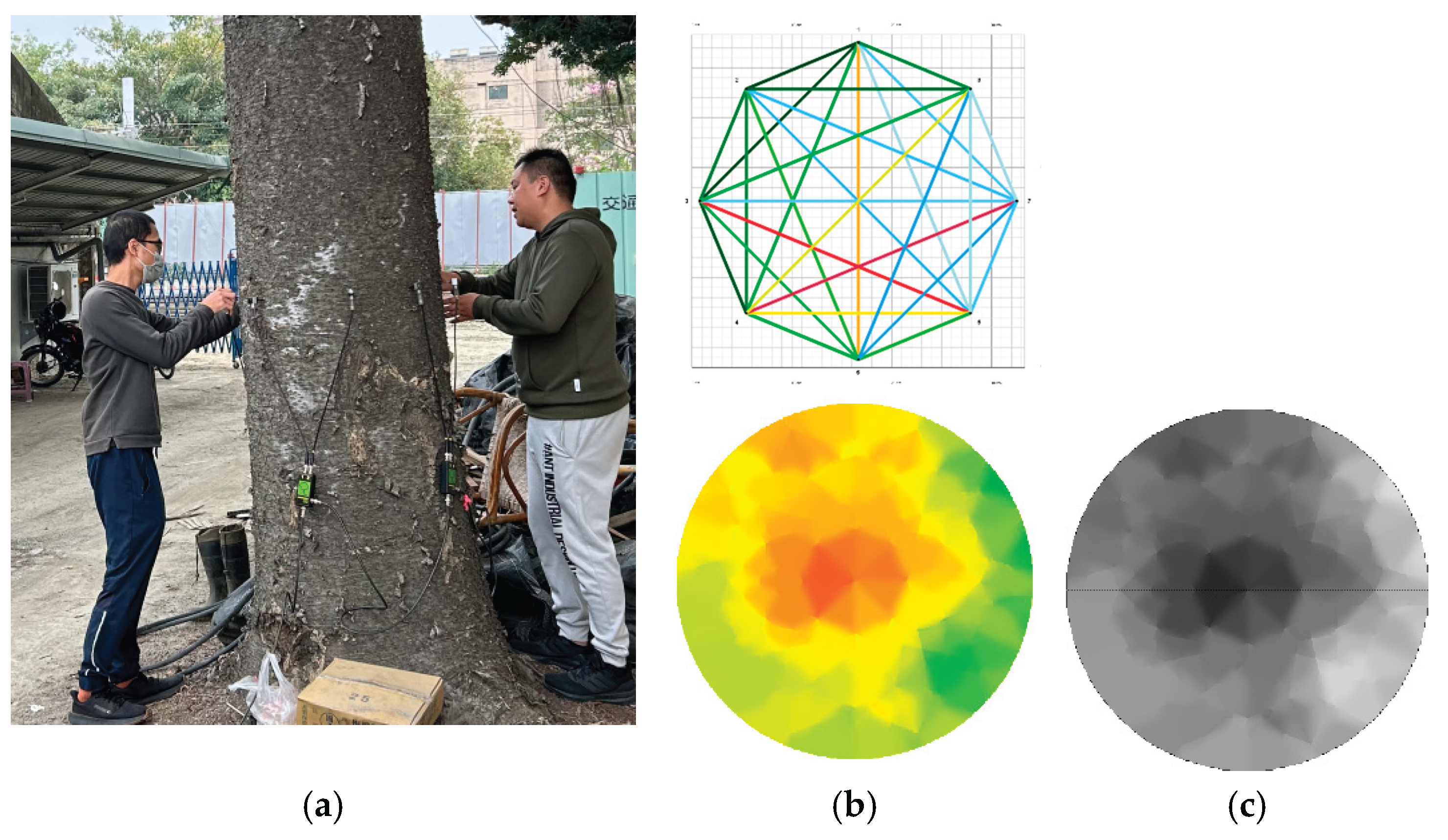
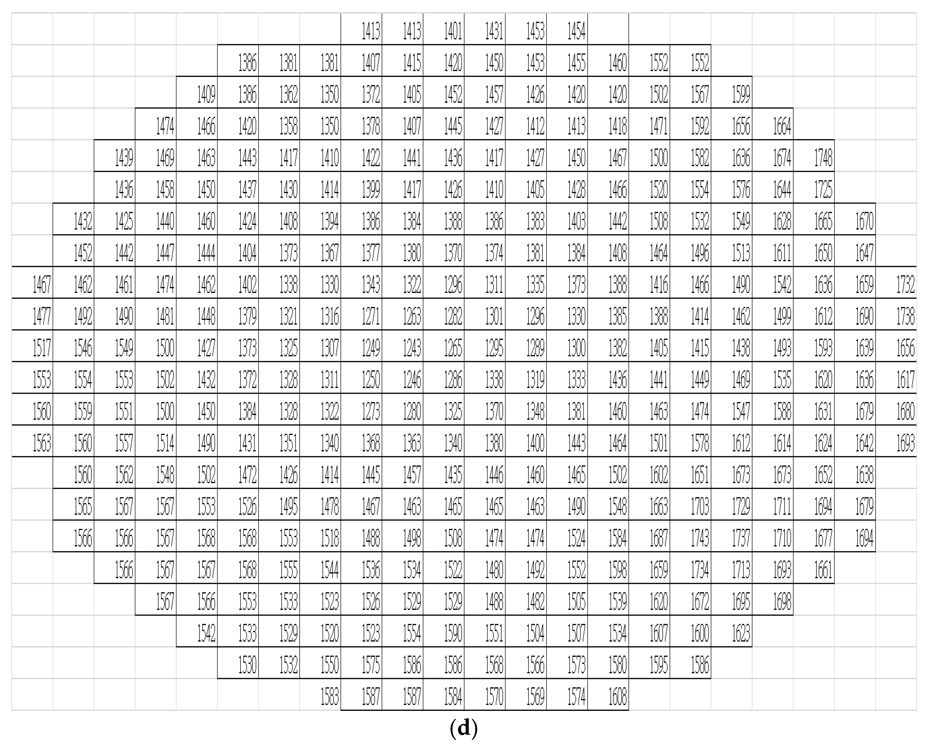
Figure 2.
Drilling amplitude profiles across four orientations (N, W, S, E) from bark to trunk center in sampled living trees.
Figure 2.
Drilling amplitude profiles across four orientations (N, W, S, E) from bark to trunk center in sampled living trees.
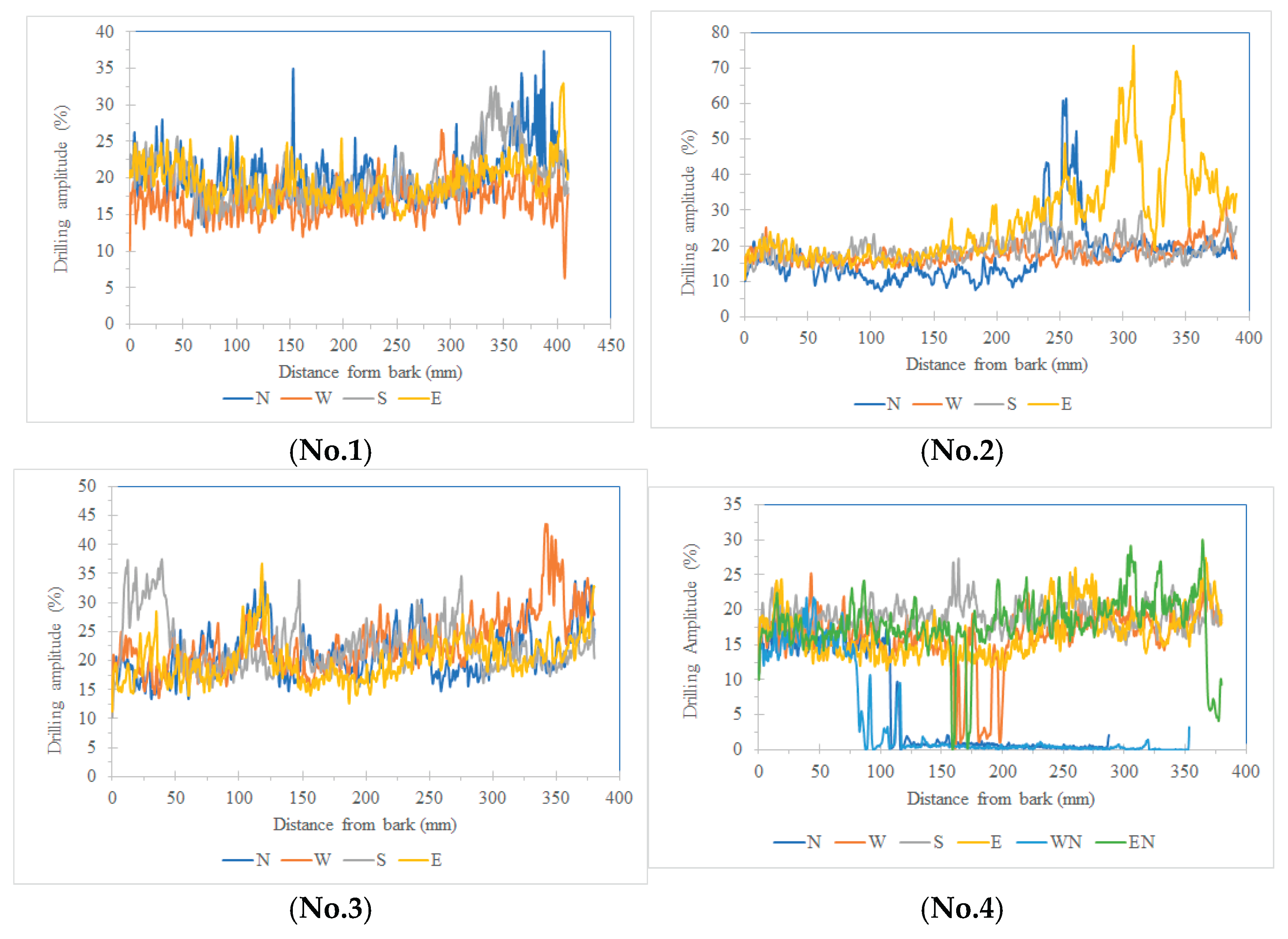
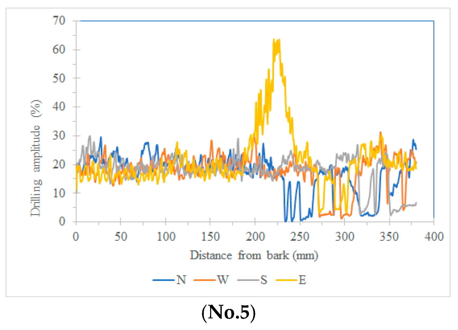
Figure 3.
Variation Trend of Stress Wave Velocity from Bark to Pith (Radial Direction) in the 2D Acoustic Tomography of Tree (No. 1). Note 1: W, Western; N, Northern; E, Eastern; Southern Orientation. Note 2: ●, 8 sensors; □, 12 sensors; △, 16 sensors; ○, 20 sensors. Note 3: 2D Acoustic Tomography with different sensor quantities, as detailed in Table 2.

Figure 4.
Variation Trend of Stress Wave Velocity from Bark to Pith (Radial Direction) in the 2D Acoustic Tomography of Tree (No. 2). Note 1: W, Western; N, Northern; E, Eastern; Southern Orientation. Note 2: ●, 8 sensors; □, 12 sensors; △, 16 sensors; ○, 20 sensors. Note 3: 2D Acoustic Tomography with different sensor quantities, as detailed in Table 2.
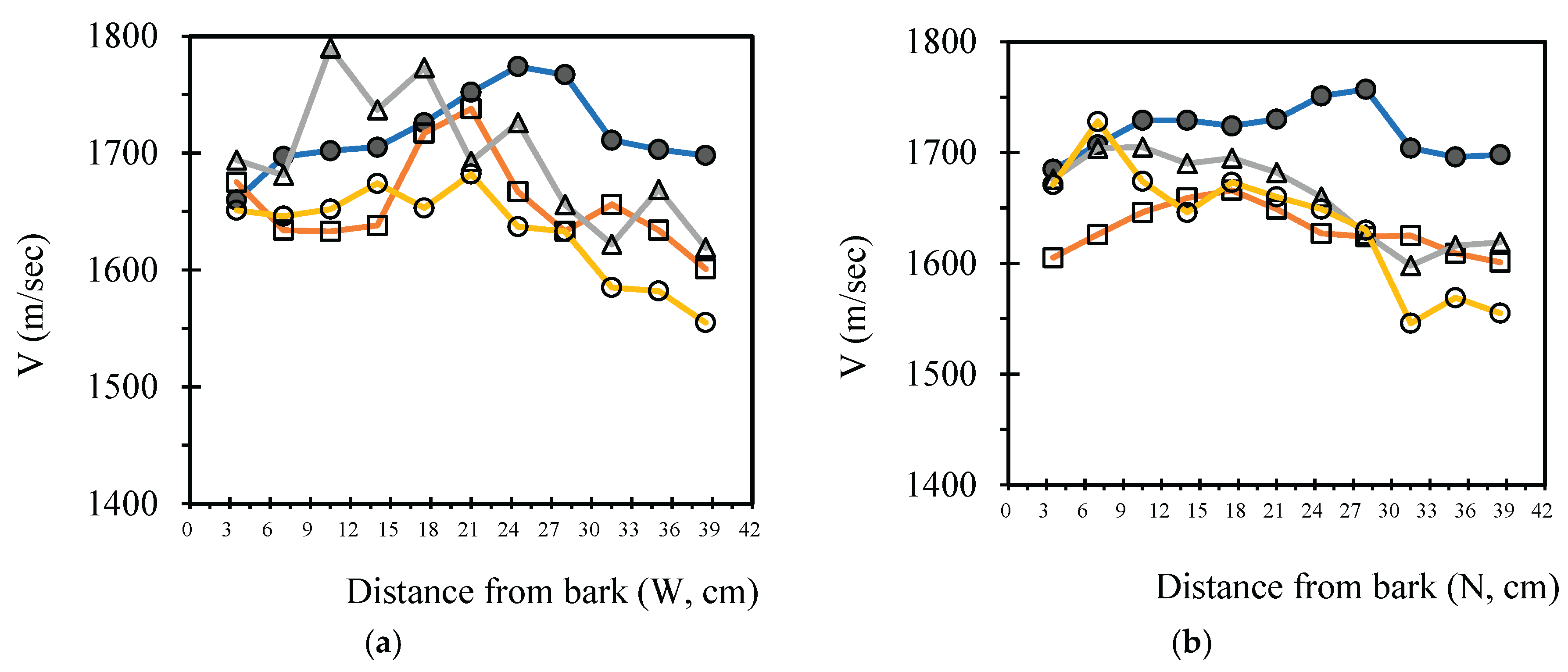
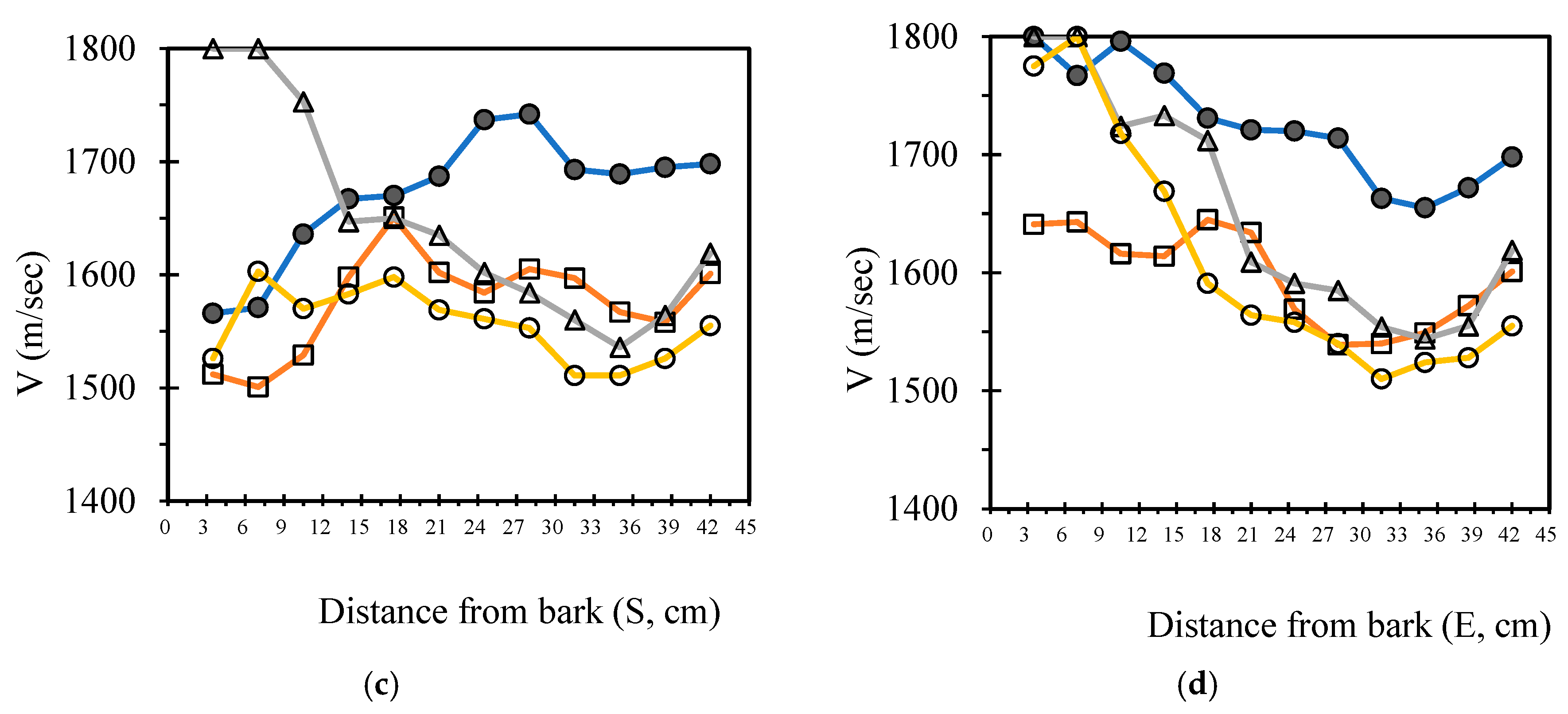
Figure 5.
Variation Trend of Stress Wave Velocity from Bark to Pith (Radial Direction) in the 2D Acoustic Tomography of Tree (No.3). Note 1: W, Western; N, Northern; E, Eastern; Southern Orientation. Note 2: ●, 8 sensors; □, 12 sensors; △, 16 sensors; ○, 20 sensors. Note 3: 2D Acoustic Tomography with different sensor quantities, as detailed in Table 2.
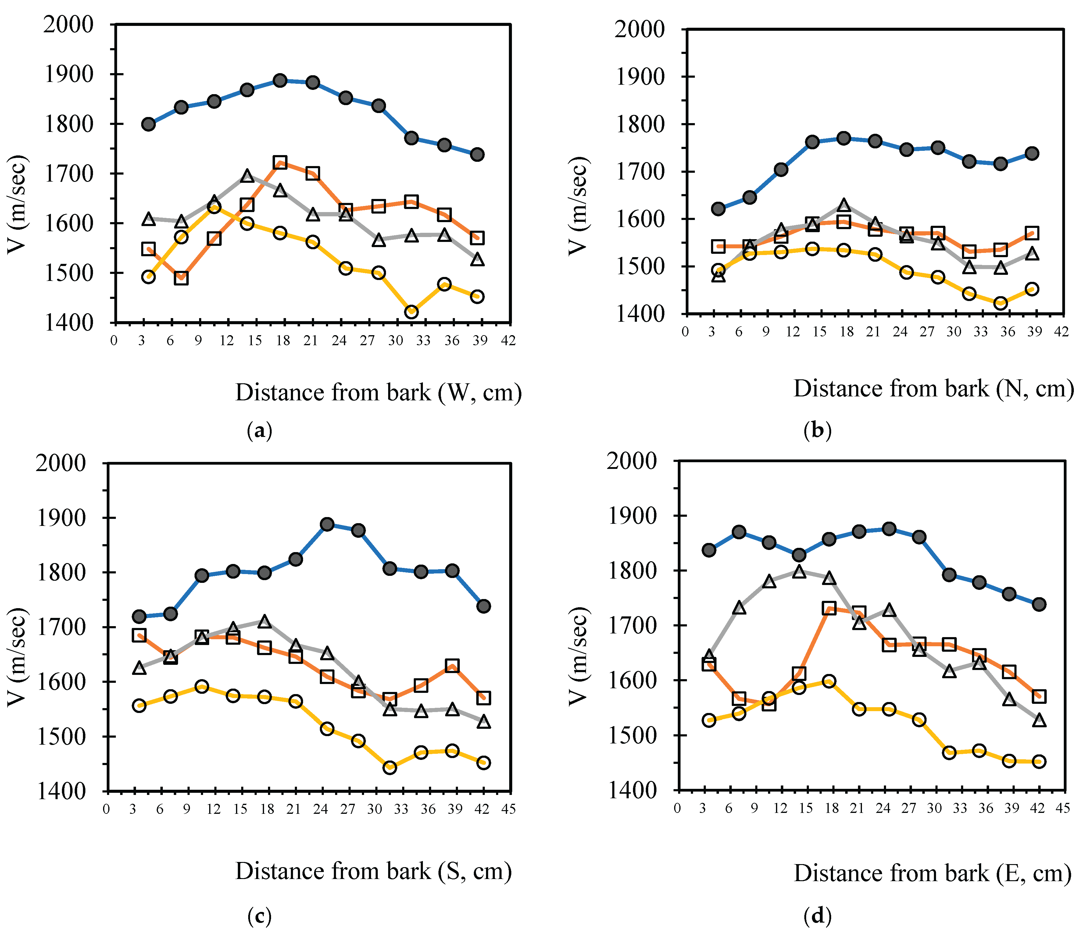
Figure 6.
Variation Trend of Stress Wave Velocity from Bark to Pith (Radial Direction) in the 2D Acoustic Tomography of Tree (No. 4). Note 1: W, Western; N, Northern; E, Eastern; Southern Orientation. Note 2: ●, 8 sensors; □, 12 sensors; △, 16 sensors; ○, 20 sensors. Note 3: 2D Acoustic Tomography with different sensor quantities, as detailed in Table 2.
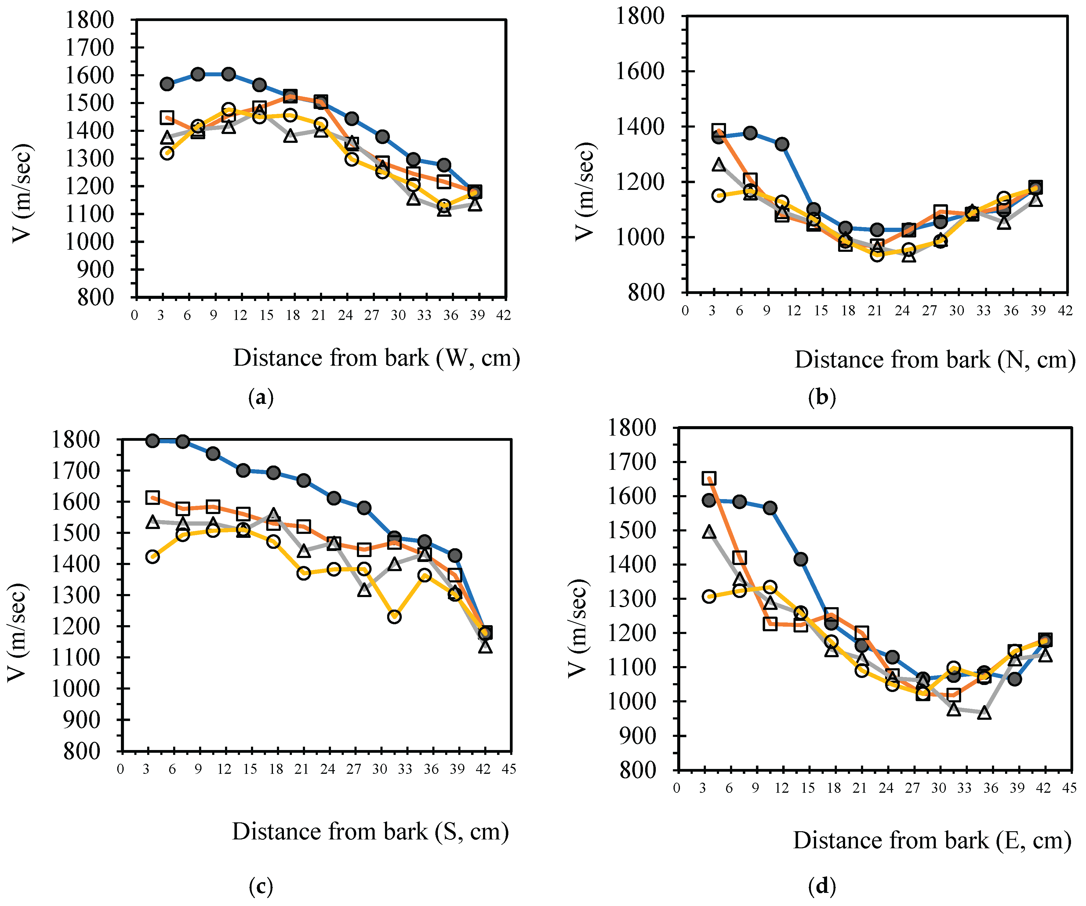
Figure 7.
Variation Trend of Stress Wave Velocity from Bark to Pith (Radial Direction) in the 2D Acoustic Tomography of Tree (No. 5). Note 1: W, Western; N, Northern; E, Eastern; Southern Orientation. Note 2: ●, 8 sensors; □, 12 sensors; △, 16 sensors; ○, 20 sensors. Note 3: 2D Acoustic Tomography with different sensor quantities, as detailed in Table 2.
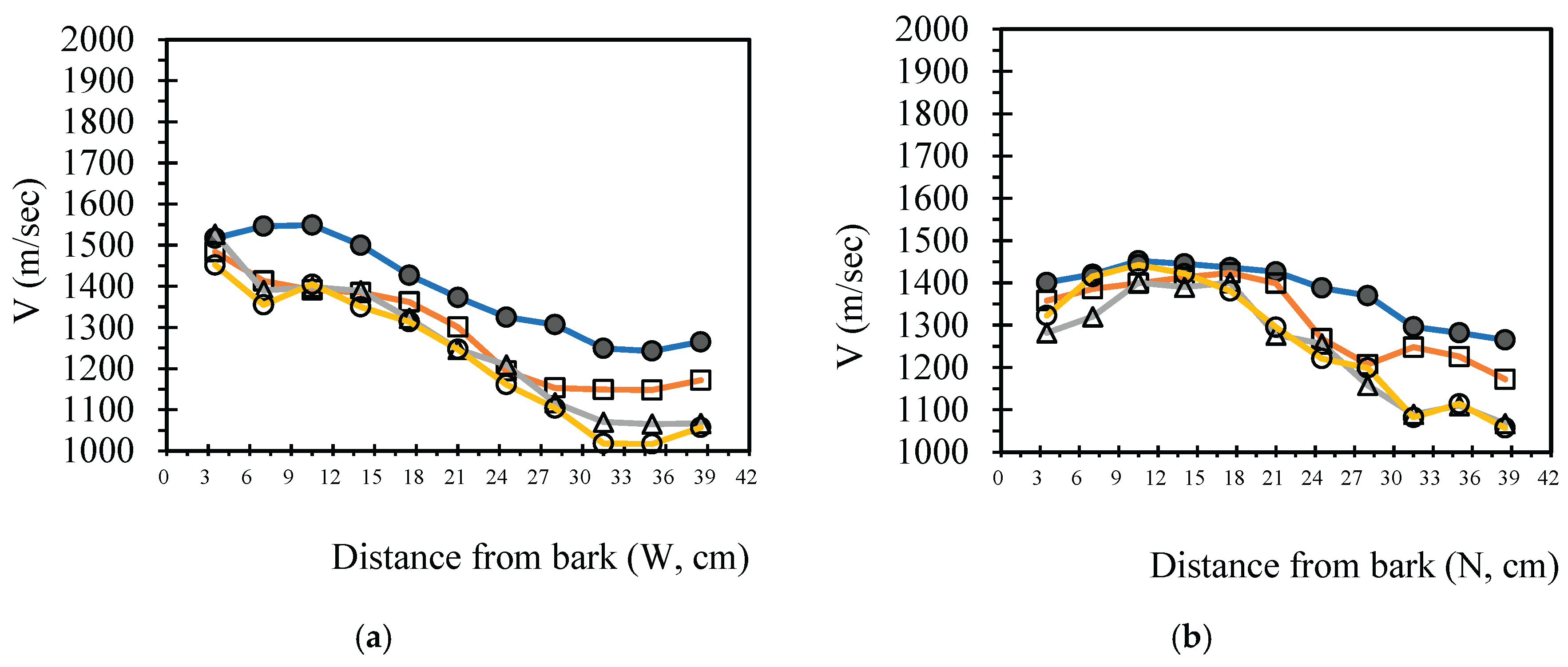
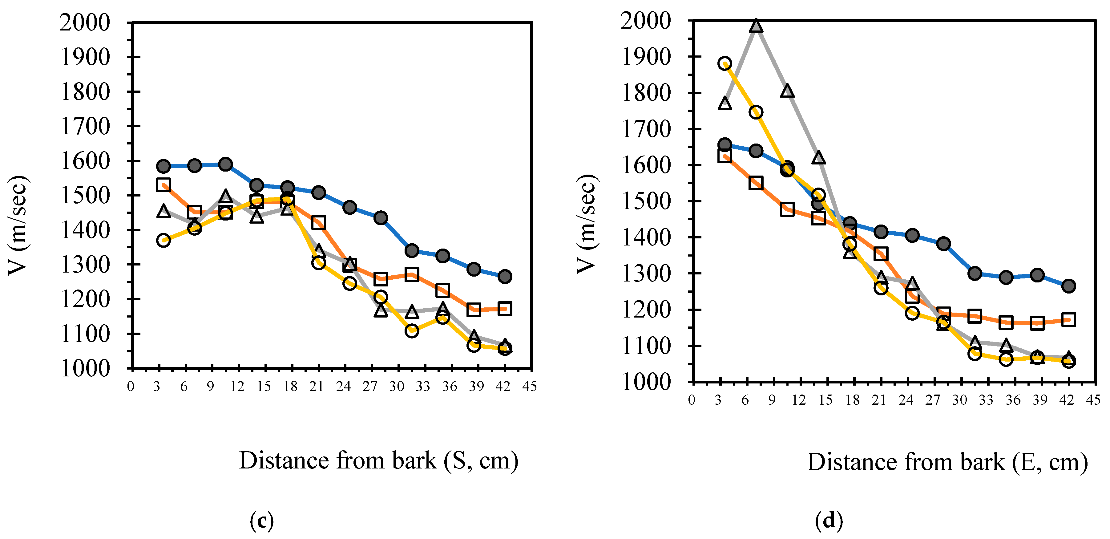
Table 2.
Maximum, Minimum, and Average Stress Wave Velocity of 2D Acoustic Tomography (m/sec).
| Sampled tree | Diameter of 2D (cm) | Numbers of Sensors | V (m/sec) | 2D | ||
|---|---|---|---|---|---|---|
| V max | V min | V mean | ||||
| No. 1 | 82.2 | 8 | 1793 | 1319 | 1556 |  |
| 12 | 1744 | 1126 | 1435 |  |
||
| 16 | 1841 | 1183 | 1512 |  |
||
| 20 | 1883 | 1091 | 1487 |  |
||
| Average | 1815.3 | 1179.8 | 1497.5 | |||
| SD | 60.1 | 100.3 | 50.5 | |||
| No. 2 | 78.7 | 8 | 2342 | 1338 | 1840 |  |
| 12 | 1830 | 1123 | 1476 |  |
||
| 16 | 2251 | 970 | 1610 |  |
||
| 20 | 2031 | 981 | 1506 |  |
||
| Average | 2113.5 | 1103.0 | 1608.0 | |||
| SD | 229.7 | 171.5 | 165.0 | |||
| No. 3 | 76.4 | 8 | 1992 | 1396 | 1694 |  |
| 12 | 1894 | 1154 | 1524 |  |
||
| 16 | 1853 | 1207 | 1530 |  |
||
| 20 | 1768 | 970 | 1369 |  |
||
| Average | 1876.8 | 1181.8 | 1529.3 | |||
| SD | 93.0 | 175.3 | 132.7 | |||
| No. 4 | 76.4 | 8 | 1894 | 946 | 1420 |  |
| 12 | 2404 | 873 | 1638 |  |
||
| 16 | 2055 | 857 | 1456 |  |
||
| 20 | 1605 | 828 | 1216 |  |
||
| Average | 1989.5 | 876.0 | 1432.5 | |||
| SD | 333.2 | 50.2 | 173.0 | |||
| No. 5 | 76.4 | 8 | 1883 | 1102 | 1492 |  |
| 12 | 1904 | 998 | 1451 |  |
||
| 16 | 2384 | 918 | 1651 |  |
||
| 20 | 2204 | 884 | 1544 |  |
||
| Average | 2093.8 | 975.5 | 1534.5 | |||
| SD | 242.8 | 96.9 | 86.5 | |||
Note 1: Vmax, maximum stress wave velocity; Vmean, mean stress wave velocity; Vmin, minimum stress wave velocity; SD, standard deviation; Note 2: Stress wave velocity tomography using a green–yellow–red color scale (Vmax–Vmean–Vmin): Green represents the highest velocity, yellow indicates medium velocity, and red denotes the lowest velocity.
Table 3.
Average Stress Wave Velocity of 2D Acoustic Tomographies with different numbers of sensors After Gridding (m/s).
Table 3.
Average Stress Wave Velocity of 2D Acoustic Tomographies with different numbers of sensors After Gridding (m/s).
| Numbers of sensors | 8 | 12 | 16 | 20 |
|---|---|---|---|---|
| No.1 (n=421) | ||||
| Average | 1644.4a | 1585.8b | 1581.6b | 1565.7c |
| SD | 56.3 | 64.1 | 58.6 | 52.0 |
| No.2 (n=384) | ||||
| Average | 1740.1a | 1614.8c | 1712.4b | 1624.1c |
| SD | 101.8 | 71.9 | 124.6 | 76.2 |
| No.3 (n=384) | ||||
| Average | 1796.5a | 1633.8b | 1659.3c | 1549.4d |
| SD | 71.3 | 77.6 | 77.5 | 48.8 |
| No.4 (n=384) | ||||
| Average | 1494.9a | 1436.3b | 1336.2c | 1299.3c |
| SD | 230.1 | 268.7 | 195.5 | 172.9 |
| No.5 (n=384) | ||||
| Average | 1490.2a | 1423.3b | 1403.7bc | 1395.3c |
| SD | 111.4 | 121.5 | 184.4 | 162.4 |
In the given column, different letters (such as a, b, c) indicate significant differences (p ≦ 0.05), as determined by the ANOVA Tukey test.
Table 4.
Coefficients of Linear Regression Formulas (Y=AX+B) for the Correlation Between Stress Wave Velocities from Different numbers of Sensors in 2D Acoustic Tomography.
Table 4.
Coefficients of Linear Regression Formulas (Y=AX+B) for the Correlation Between Stress Wave Velocities from Different numbers of Sensors in 2D Acoustic Tomography.
| Coefficients | R2 | F value | ||||
|---|---|---|---|---|---|---|
| Y | X | A | B | |||
| No. 1 | 12 sensors | 8 sensors | 0.71 | 422 | 0.49 | 44.7** |
| 16 sensors | 8 sensors | 0.58 | 616 | 0.33 | 22.6** | |
| 20 sensors | 8 sensors | 0.18 | 1268 | 0.06 | 2.8-- | |
| 16 sensors | 12 sensors | 0.69 | 480 | 0.47 | 40.6** | |
| 20 sensors | 12 sensors | 0.41 | 905 | 0.31 | 21.1** | |
| 20 sensors | 16 sensors | 0.45 | 857 | 0.37 | 27.2** | |
| No. 2 | 12 sensors | 8 sensors | 0.62 | 550 | 0.37 | 25.8** |
| 16 sensors | 8 sensors | 0.09 | 1506 | <0.01 | 0.15-- | |
| 20 sensors | 8 sensors | 0.81 | 224 | 0.29 | 18.4** | |
| 16 sensors | 12 sensors | 0.44 | 956 | 0.08 | 3.8-- | |
| 20 sensors | 12 sensors | 0.86 | 220 | 0.35 | 23.5** | |
| 20 sensors | 16 sensors | 0.67 | 488 | 0.52 | 47.6** | |
| No. 3 | 12 sensors | 8 sensors | 0.41 | 882 | 0.21 | 11.9** |
| 16 sensors | 8 sensors | 0.81 | 167 | 0.44 | 34.9** | |
| 20 sensors | 8 sensors | 0.37 | 846 | 0.20 | 11.0** | |
| 16 sensors | 12 sensors | 0.75 | 414 | 0.29 | 18.3** | |
| 20 sensors | 12 sensors | 0.38 | 904 | 0.16 | 8.5** | |
| 20 sensors | 16 sensors | 0.52 | 670 | 0.58 | 61.1** | |
| No. 4 | 12 sensors | 8 sensors | 0.76 | 248 | 0.87 | 286** |
| 16 sensors | 8 sensors | 0.74 | 230 | 0.92 | 483** | |
| 20 sensors | 8 sensors | 0.63 | 373 | 0.87 | 300** | |
| 16 sensors | 12 sensors | 0.92 | 65 | 0.93 | 610** | |
| 20 sensors | 12 sensors | 0.75 | 266 | 0.83 | 213** | |
| 20 sensors | 16 sensors | 0.82 | 241 | 0.89 | 340** | |
| No. 5 | 12 sensors | 8 sensors | 1.05 | -168 | 0.87 | 289** |
| 16 sensors | 8 sensors | 1.65 | -1037 | 0.82 | 202** | |
| 20 sensors | 8 sensors | 1.55 | -913 | 0.84 | 230** | |
| 16 sensors | 12 sensors | 1.45 | -624 | 0.82 | 195** | |
| 20 sensors | 12 sensors | 1.41 | -586 | 0.89 | 355** | |
| 20 sensors | 16 sensors | 0.89 | 126 | 0.91 | 462** | |
R2, Coefficient of determination; * P < 0.05; ** P < 0.01; -- P ≧0.05.
Table 5.
Average Stress Wave Velocity in Healthy and Damaged Zones Using 2D Acoustic Tomography with Different Numbers of Sensors Post-Gridding (Unit: m/s).
Table 5.
Average Stress Wave Velocity in Healthy and Damaged Zones Using 2D Acoustic Tomography with Different Numbers of Sensors Post-Gridding (Unit: m/s).
| Numbers of sensors | 8 | 12 | 16 | 20 |
|---|---|---|---|---|
| No.4 | ||||
| Health zones (n=333) | ||||
| Average | 1553.2 | 1448.1 | 1378.2 | 1336.8 |
| SD | 174.7 | 241.9 | 166.2 | 145.5 |
| Damaged zones (n=51) | ||||
| Average | 1055.2 | 1046.0 | 1019.6 | 1017.3 |
| SD | 48.9 | 52.8 | 65.8 | 92.0 |
| No.5 | ||||
| Health zones (n=348) | ||||
| Average | 1506.9 | 1442.9 | 1430.0 | 1420.9 |
| SD | 101.7 | 107.8 | 171.6 | 144.4 |
| Damaged zones (n=36) | ||||
| Average | 1309.3 | 1206.2 | 1119.8 | 1105.9 |
| SD | 44.2 | 39.3 | 48.2 | 58.8 |
Disclaimer/Publisher’s Note: The statements, opinions and data contained in all publications are solely those of the individual author(s) and contributor(s) and not of MDPI and/or the editor(s). MDPI and/or the editor(s) disclaim responsibility for any injury to people or property resulting from any ideas, methods, instructions or products referred to in the content. |
© 2025 by the authors. Licensee MDPI, Basel, Switzerland. This article is an open access article distributed under the terms and conditions of the Creative Commons Attribution (CC BY) license (http://creativecommons.org/licenses/by/4.0/).
Copyright: This open access article is published under a Creative Commons CC BY 4.0 license, which permit the free download, distribution, and reuse, provided that the author and preprint are cited in any reuse.


