
Submitted:
29 August 2025
Posted:
01 September 2025
You are already at the latest version
Abstract
This paper presents a novel DC microgrid configuration tailored for residential applications, aiming to harness renewable energy and enhance resilience against the growing threats of natural disasters and cyber-physical attacks—factors that increasingly expose the fragility of existing power grid systems. The proposed system employs autonomous decentralized cooperative control and introduces a distinctive battery-integrated DC-baseline architecture, wherein distributed batteries are directly connected to the grid’s baseline. This topology streamlines control: distributed batteries directly connected to the baseline handle forming and maintaining core grid, while DC/DC converters are dedicated solely to power exchange between power devices. A key factor is to employ weak-coupling grid for realizing autonomous decentralized control. By using the configuration, the system minimizes inter-device interference, thereby obtaining control independence of local devices. Comprehensive MATLAB/Simulink simulations of a four-house DC microgrid—modeled on a typical Japanese residential setting—demonstrate that an optimal configuration with 5 kW solar panels and 20 kWh batteries per household can achieve a renewable energy ratio exceeding 50%, while maintaining stable grid operation year-round, even with electric vehicle charging. The proposed system offers a balanced design with an estimated battery lifetime of approximately 25 years, paving the way for sustainable, resilient, and locally governed energy infrastructures.
Keywords:
DC grid
; Residential microgrid
; Autonomous decentralized cooperative control
; Weak-coupling grid
1. Introduction
The power grid, alongside communication networks, water supply systems, and city gas infrastructure, is a vital lifeline of modern society. However, its vulnerabilities have become increasingly apparent in recent years due to the intensification of natural disasters and its susceptibility to targeted attacks such as terrorism and warfare [1,2,3]. Existing power grids typically rely on large-scale generation at power plants located far from urban centers—the primary consumers of electricity—and transmit power over long distances via transmission and distribution lines. This centralized structure introduces multiple points of fragility, particularly in large facilities and extended transmission pathways, making the system vulnerable to disruptions. In contrast, microgrids—comprising small-scale distributed energy resources such as solar, wind, and hydro generators, along with batteries—are gaining attention for their resilience [4,5]. These systems incorporate distributed energy sources into the grid and operate locally, generating and storing only the necessary amount of electricity near the point of consumption. Microgrids fundamentally reject the premise of long-distance power transmission, instead promoting “local production and consumption of electricity”.
As such, microgrids and conventional power grids are based on fundamentally different philosophies. Table 1 compares the two systems, highlighting differences not only in their conceptual approach to electricity usage but also in the types of power handled, grid topology, and control methods. Conventional grids employ high-voltage AC suitable for long-distance transmission, whereas microgrids handle low-voltage DC or AC, which is more accessible for power consumers. Topologically, conventional grids follow a river-flow (tree) structure flowing from upstream generators to downstream consumers, while microgrids typically adopt a bus-type configuration, allowing for diverse topologies. Control methods also differ significantly. Conventional grids rely on centralized control by utility companies, whereas microgrids may incorporate autonomous decentralized cooperative control in addition to centralized schemes. Moreover, conventional grids are designed without power storage, requiring instantaneous balance between power generation and consumption (the principle of simultaneous supply and demand). Grid stability during short time scales depends on electrical inertia provided by upstream generators, which propagates through the transmission line to downstream loads, ensuring reliable operation of electrical devices. This necessitates strong electrical coupling between generators and end-use devices.
Microgrids, too, require electrical inertia for grid stability, but this is provided by distributed sources such as batteries. Typically, DC/DC converters or DC/AC inverters connected to these batteries emulate inertia to stabilize the grid [6,7]. As a result, multiple sources of electrical inertia are located near the loads, enabling the possibility of a weakly coupled grid structure, as discussed in Section 4.
In summary, conventional power grids and microgrids differ fundamentally. While parts of the conventional grid—particularly downstream segments—may be replaced by microgrids in the future, a complete replacement is unlikely. Instead, the two systems are expected to coexist, complementing each other’s weaknesses.
Microgrids can be implemented in both AC and DC formats. Conventional AC microgrids typically operate by borrowing or extending utility distribution grids during normal conditions and switching to islanded operation during disasters. Thus, they are essentially an extension of the utility grid.
In contrast, DC microgrids are built with independent grids separate from the utility grid, making them fundamentally distinct. This independence allows DC microgrids to employ autonomous decentralized cooperative control [8,9], a method that eliminates centralized controllers and communication lines between devices. Such a configuration significantly enhances disaster resilience, as even if part of the grid is damaged, the remaining segments can maintain partial functionality. For this autonomous operation, each power device must make independent decisions based on its local assessment of grid conditions, such as baseline voltage. This necessitates sophisticated self-regulation, often performed by DC/DC converters connected to distributed power sources or by the power loads themselves. Since devices do not have a global view of the grid, optimization is limited to local performance rather than system-wide coordination, making autonomous decentralized cooperative control inherently a form of local control. Section 4 provides a detailed explanation of how this local control is implemented within DC microgrids.
This paper investigates the design and operation of a DC microgrid for typical residential areas, in which individual homes are interconnected via a shared DC baseline. We focus on deployment in Japanese communities, where disaster resilience is particularly critical due to the country’s high exposure to natural hazards. Each home is assumed to be equipped with small-scale photovoltaic (PV) panels and batteries. The system is designed to exhibit resilience during disasters through autonomous decentralized control, while under normal conditions, it supports an eco-conscious lifestyle by prioritizing the use of renewable energy wherever possible. We evaluate grid stability, the required capacities for solar panels and batteries, energy exchange with the utility grid, and renewable energy ratio under normal operating conditions. Since solar power generation is inherently intermittent, it is not feasible to maintain a stable lifestyle relying solely on renewable sources. Therefore, a minimum amount of electricity is procured from the utility grid, and this is kept as low as possible.
2. Battery-Integrated DC Baseline
We previously proposed a DC grid architecture in which batteries are directly connected to the grid baseline [10]. In conventional DC microgrids, as illustrated in Figure 1(a), batteries are typically connected to the baseline via DC/DC converters. These converters play a critical role in maintaining and stabilizing the grid, including the provision of pseudo-inertial characteristics. However, when a DC/DC converter is interposed, the battery’s inherent electrical inertia cannot be fully transmitted to the baseline due to limitations imposed by the converter’s rated power capacity. Moreover, its electronic control introduces delays on the order of several milliseconds, during which certain power-load equipment may experience instability or even shut down.
To address this issue, we proposed a method for directly connecting batteries to the grid baseline, as shown in Figure 1(b), thereby transmitting their electrical inertia without degradation. Specifically, batteries are configured such that their terminal voltage closely matches the baseline voltage, enabling direct connection. When batteries are directly connected to the baseline, their intrinsic droop characteristics with respect to terminal voltage naturally facilitate coordinated operation among multiple batteries [10].
This configuration—where multiple small batteries are distributed and directly connected to the baseline—forms a battery-integrated DC baseline. It allows the fundamental grid-forming and sustaining functions to be handled by the distributed batteries themselves, without relying on DC/DC converters.
Inspired by the open systems interconnection (OSI) reference model [11] for communication networks, we define the grid functionality across four hierarchical layers, as shown in Table 2.
- -
- **Layer 1: Physical Layer**
This layer specifies the physical medium and standards for power exchange among devices connected to the grid. Common media include CV cables, with specifications covering conductor type, thickness, number of cores, insulation type, and grounding methods.
- -
- **Layer 2: Grid Forming Layer**
This layer governs the essential functions for forming and maintaining the grid at a specified voltage. It defines the type of power (AC or DC), voltage range, frequency, and phase configuration (single-phase or three-phase). Mechanisms for electrical inertia, droop control for coordinated operation of distributed power sources, and power distribution balancing are included. Protection against ground faults, short circuits, and lightning strikes is also specified. In conventional DC grid, these functions are typically handled by DC/DC converters connected to distributed sources.
- -
- **Layer 3: Power Exchange Layer**
This layer defines the mechanisms for power exchange between power devices and the grid, as well as between the grid and external systems such as utility grids or other microgrids. DC/DC or DC/AC converters are responsible for these functions.
- -
- **Layer 4: Application Layer**
This top layer encompasses various applications that utilize the grid, such as energy management systems (EMS) or electricity trading platforms.
Table 3 compares devices responsibilities for each grid function between conventional DC microgrids and battery-integrated DC microgrids. In conventional DC grids, both Layer 2 (grid forming) and Layer 3 (power exchange) functions are handled by DC/DC converters. In contrast, the battery-integrated grid delegates Layer 2 functions to the distributed batteries directly connected to the baseline, allowing DC/DC converters to focus solely on Layer 3 functions. This separation simplifies control.
Figure 2 illustrates the devices responsible for each layer in both conventional and battery-integrated grids. In conventional DC grids, DC/DC converters connected to distributed sources must manage a wide range of controls across Layers 2 and 3, resulting in high complexity and control burden. To mitigate this, hierarchical control schemes have been proposed to prioritize control tasks and prevent interference [12,13].
In our battery-integrated baseline approach, these roles are clearly separated and simplified. Grid forming (Layer 2) is entrusted to the directly connected batteries, while DC/DC converters concentrate on power exchange (Layer 3). This significantly reduces the complexity of DC/DC converter control.
4. Autonomous Decentralized Cooperative Control Realized by Weakly Coupled Grid Configuration
In conventional power grids, electrical inertia must be transmitted from upstream power generators to downstream power loads. To achieve this, the system relies on thick, high-capacity transmission and distribution lines operating at high voltages. In contrast, typical DC microgrids operate at relatively low voltages—around 400 V—baseline and their baseline power capacity are modest. This difference stems primarily from the relative positioning of the sources of electrical inertia and the power loads.
Figure 3 compares the magnitude of electrical inertia along the baseline between Japan’s conventional distribution grid (6.6 kV) and a DC microgrid (baseline voltage: 400 V). Here, the magnitude of electrical inertia is defined as the maximum instantaneous power that can be extracted at a given point on the baseline. Due to the conductor resistance of the baseline cable, the electrical inertia decreases with distance from the inertia source, but near the inertia source, the magnitude is limited by the allowable current capacity of the baseline cable. Japan’s distribution grid uses relatively thick cables (22–150 square millimeters (SQ)) at 6.6 kV, allowing substantial electrical inertia to be transmitted even over distances exceeding 10 km. In contrast, DC microgrids use thinner cables (typically 8–14 SQ) at around 400 V, resulting in significantly lower electrical inertia and a more limited range of influence. However, because sources of electrical inertia—such as distributed batteries—are located near the power loads, even such weakly coupled grid can effectively distribute sufficient inertia across the baseline.
Weak coupling is also essential for implementing autonomous decentralized cooperative control. In this control paradigm, each device must operate independently without interference from neighboring devices, necessitating strictly local control. Typically, a device senses the grid state—such as the baseline voltage—at its connection point to the grid and determines its behavior accordingly. If the operation of adjacent devices affects this sensing, accurate assessment of the grid state becomes impossible (see Figure 4a). Strong electrical coupling through the baseline increases the likelihood of such interference.
To quantify this, a simplified equivalent circuit of a battery-integrated weakly-coupled DC grid is shown in Figure 4b. Here, R represents the conductor resistance of the baseline between devices, C denotes the dynamic capacitance of the battery, and τ is the time constant of device control—typically less than several second, as seen in solar panel MPPT charging control systems.
The conductor resistance R reflects the strength of coupling between devices. In weakly coupled grids, R is non-negligible, typically ranging from 0.1 to 1 Ω. The dynamic capacitance C of the battery is defined by the following equation:
where dq is the change in charge and dV is the resulting change in terminal voltage. Depending on battery type and capacity, C can be extremely large. For example, a 48 V, 40 Ah lithium iron phosphate battery yields a capacitance exceeding 1,000 F. Thus, the CR time constant, determined by the battery capacitance and conductor resistance, is typically much larger than the device control time constant τ, as indicated by the following inequality:
This ensures the independence of each device’s control, enabling effective local regulation. Although the control actions of neighboring devices may influence the sensing point via the baseline, such effects occur on a slower timescale than the control response of devices, preserving control autonomy.
Even in weakly coupled grids, gradual power exchange between devices remains feasible. Therefore, if a state-of-charge (SoC) imbalance arises among distributed batteries directly connected to the baseline, it will naturally self-balance over time [14]. Additionally, when a large power load—such as EV charging—is introduced, the local baseline voltage may begin to drop. However, the resulting voltage differential induces a compensating current flow, suppressing the voltage drop and stabilizing it at a fixed level.
5. Simulation Model for a residential Microgrid
To analyze the long-term operation of the battery-integrated, weakly coupled DC microgrid, we developed a simulation model using MATLAB/Simulink. Device models were constructed based on simplified electric equivalent circuits to emulate the behavior of lithium iron phosphate (LiFePO₄) batteries, silicon solar panels, and residential electricity consumption. The solar panel model outputs real-time power generation based on input parameters including the panel’s rated capacity, global solar radiation at the installation site, ambient temperature, and installation efficiency. Historical meteorological data for major Japanese cities were obtained from the Japan Meteorological Agency’s website [15]. Residential electricity consumption was statistically modeled based on the average monthly energy usage of a typical four-person household in Japan (Table 4) [16], combined with the hourly consumption profile shown in Figure 5 [17]. Although seasonal variations exist, an annual average profile was adopted for simplification. To reflect household-level variability, random fluctuations were introduced into each home’s power demand. For power cables, including grid baselines, only conductor resistance—determined by the thickness and length of the core wire—was considered. Inductance and inter-wire capacitance were ignored. All power devices operate autonomously without centralized control. Although the input statistical data have an hourly resolution, the simulation was conducted over a one-year period with a time step of one second (60 × 60 × 24 × 365 = 31,536,000 steps).
The simulation scenario assumes the construction of a DC microgrid in a residential area of Sendai, Japan, aiming to realize an environmentally friendly lifestyle based on local generation and consumption of solar energy. Figure 6 illustrates the simulation model developed using the MATLAB/Simulink platform. Four houses, each equipped with a 5 kW solar panel and a 50 Ah battery (approximately 20 kWh capacity), are connected via a bus-type DC baseline. One end of the baseline (left end) is connected to the utility distribution grid.
The baseline voltage is centered at 380 V, with an allowable operating range of ±10%, i.e., 340 V to 420 V. All power-load devices, generation units, and storage systems are assumed to operate normally within this voltage range. Each device model monitors the voltage at its connection point (baseline voltage) and operates autonomously and in a decentralized manner because centralized controller is not present. Therefore, if the baseline voltage remains within the allowable range, autonomous decentralized cooperative control is considered to be functioning properly.
Power exchange with the utility grid is governed by the following rules:
- -
- When the baseline voltage drops below 360 V, the microgrid begins receiving power from the utility grid at a fixed rate, continuing until the voltage recovers to 370 V.
- -
- When the baseline voltage exceeds 400 V, the microgrid begins sending power to the utility grid at a fixed rate, continuing until the voltage drops to 390 V.
- -
- Outside these conditions, no power exchange occurs.
This control scheme ensures that the baseline voltage remains within the permissible range, even during periods of low solar generation or excess production.
While the widespread deployment of electric vehicle (EV) chargers has raised concerns about their impact on the power grid [18], home-based EV charging is also expected to pose significant challenges for microgrid operation in the near future. Accordingly, we considered a scenario in which House 3 (the third house from the left) is equipped with EV charging infrastructure.
The baseline connecting the houses consists of CV cables with a conductor thickness of 8 SQ, and each segment is uniformly set to 50 meters in length. Table 5 summarizes the specifications of the microgrid. The installation efficiency of the solar panels—determined by factors such as orientation and tilt angle—is uniformly assumed to be 50%.
6. Simulation Results
6.1. Without EV Charging Infrastructures
We first examined the case without electric vehicle (EV) charging infrastructure. Figure 7 shows the annual variation and a detailed view of the January monthly variation in the power generated by the solar panel installed on each house. Since all houses are located within a 100-meter radius, we assumed uniform solar irradiance across all PV installations. Power generation peaks between April and May, decreases during the rainy season (June–July), and is slightly lower in August due to high ambient temperatures. In winter (December–February), generation is reduced due to shorter daylight hours and snowfall.
Figure 8 illustrates the annual variation in electricity consumption across the four households, along with a detailed view of the January variation for House 4. In this graph, power consumption is represented as negative values, since power generation is defined as positive. While consumption varies by household, it statistically follows the distribution shown earlier. Higher consumption is observed in winter and summer due to air conditioning use.
Figure 9 presents the annual variation in baseline voltage at each household’s connection point. In a weakly coupled grid, baseline voltages may exhibit substantial variation even between adjacent subgrids connected via a common baseline. Although temporal fluctuations are observed, all voltages remain within the acceptable range of 340 V to 420 V. House 1, which is closest to the utility grid connection point, shows relatively minor voltage fluctuations, while houses farther away experience greater variation. In spring, elevated voltage levels are observed due to high PV generation combined with moderate consumption. In contrast, winter conditions—low generation—result in voltages trending between 360 V and 380 V. It is worth noting that in this simulation, PV output is not curtailed even when baseline voltage is high; all generated power is absorbed into the microgrid.
Figure 10 shows the charging and discharging power of the batteries installed in each house. Discharging is plotted as positive, and charging as negative. All batteries operate throughout the year, with Battery 1 (in House 1, near the grid connection point) exhibiting the most intense activity, reaching up to 4 kW. Figure 11 plots the cumulative charge/discharge current over time. Again, Battery 1 shows the highest activity, with an annual cumulative current of approximately 12 kAh. This corresponds to 120 full charge/discharge cycles for the installed 50 Ah battery. Given that lithium iron phosphate batteries typically have a cycle life of around 3,000 cycles [19,20,21], this suggests a battery lifetime of approximately 25 years.
Figure 12 displays the current flowing through the baseline cables connecting the houses. Positive current indicates flow toward the right (away from the utility grid connection point). Cables closer to the grid (e.g., Cable 1) carry more current, but the maximum remains below 20 A—well within the 65 A rating of the 8 SQ CV cables. Thus, the maximum power transmitted through the baseline is around 7 kW, which is modest relative to the total load, confirming that power exchange is gradual and the grid remains weakly coupled.
Figure 13 shows power exchange with the utility grid. Positive values indicate power received from the grid, and negative values indicate power sent to the grid. Naturally, more electricity is received from the utility grid in winter, and more electricity is sent to the utility grid from spring to summer.
Figure 14 illustrates the cumulative power consumption of the entire microgrid, along with the annual amounts of electricity imported from and exported to the utility grid. The total annual consumption amounts to 16.24 MWh, equivalent to approximately 338 kWh per household per month, which closely aligns with the statistical value shown in Table 4. An annual total of 4.86 MWh was received from the utility grid, whereas 3.08 MWh was transmitted back to it.
It is important to note that the definition of the renewable energy ratio (RER) depends on whether reverse power flow to the utility grid is permitted. The simulation was conducted under the condition that all excess power generated within the microgrid is absorbed by the utility grid through reverse power flow. In this scenario, RER is defined by Equation (3). If PV output is significantly increased, the RER can become arbitrarily large, potentially exceeding 100%. However, this approach deviates from the concept of “local production and consumption of electricity,” which emphasizes that residential microgrids should generate and consume only the amount of power required locally. In Japan, it has been reported that reverse power flow from mega-solar power plants during spring can destabilize the utility grid, often leading to generation curtailment. Therefore, from the perspective of “local production and consumption,” designing a microgrid that does not even consider reverse power flow to the utility grid might be a more natural approach. In such cases, if the storage batteries are fully charged and cannot store any more power, PV generation curtailment is implemented. The RER for this scenario, where reverse power flow to the utility grid is prevented by generation curtailment, is defined by Equation (4), and it will not exceed 100%. We present both definitions to provide a comprehensive understanding of the microgrid’s performance under different operational philosophies. The RER calculated using Equation (3), which allows reverse power flow to the utility grid, is approximately 89%, whereas the RER calculated using Equation (4), which prohibits reverse power flow, is approximately 70%.
6.2. With an EV Charging Infrastructure
Next, we simulated a scenario in which House 3 (the third house from the left in Figure 6) is equipped with EV charging infrastructure. In this case, EV charging is assumed to occur daily between midnight and 2:00 AM at a constant power of 5 kW, resulting in an energy consumption of 10 kWh per session.
Figure 15 shows the annual baseline voltage variation at each household connection point. While House 1 remains within the acceptable range throughout the year, Houses 3 and 4—farther from the grid connection—occasionally fall below the lower voltage limit, as indicated by red circles. These events occur during nighttime EV charging, suggesting that even 5 kW of power load can significantly impact a microgrid of this scale.
To mitigate this, we shifted the EV charging window to 2:00–4:00 AM, a period of lower household consumption as shown in Figure 5. Although the daily charging energy remains 10 kWh, the revised simulation (Figure 16) shows that voltage excursions below the acceptable range occur only once per year for Houses 3 and 4.
In this scenario, we also examined the current flow through the baseline using the same method as in the previous section (see Figure 12), although the corresponding graph is omitted here for brevity. As before, the cable segment closer to the utility grid carries a higher current, but the maximum remains below 20 A—similar to the scenario without EV charging.
Likewise, the annual variation in charging and discharging power of the batteries installed in each house was analyzed using the same approach as in the previous section (see Figure 10), but the raw data plots are omitted in this section for brevity. Battery 1 again exhibits the most pronounced charge/discharge activity. The cumulative current (Figure 17) reaches 12.59 kAh, corresponding to an estimated battery lifetime of approximately 24 years.
Figure 18 illustrates the cumulative power consumption of the entire microgrid, along with the amounts of electricity imported from and exported to the utility grid under the EV charging scenario. As a result of daily EV charging, the annual power consumption increases to 18.89 MWh, with grid imports rising to 8.27 MWh and exports reaching 2.74 MWh.
Based on Equation (3), which accounts for reverse power flow to the utility grid, the resulting RER is approximately 72%. In contrast, when reverse power flow is prohibited—as assumed in Equation (4)—the RER decreases to approximately 58%.
7. Consideration of Required System Capacity
This section evaluates how the capacity of household-installed batteries and solar panels affects the overall RER and grid stability. The simulation scenario builds upon the case presented in the previous section, in which House 3 is equipped with EV charging infrastructure, with daily charging scheduled from 2:00 AM to 4:00 AM.
In addition to the grid configuration—each household equipped with a 20 kWh battery and a 5 kW solar panel (installation efficiency: 50%)—alternative setup were assessed, including battery capacities of 5, 10, and 50 kWh, and solar panel rated outputs of 3 kW and 7 kW. The following four evaluation metrics were used:
1. RER calculated using Equations (3), assuming grid export
2. RER calculated using Equations (4), assuming curtailment of surplus
3. Battery lifetime
4. Grid stability
Battery lifetime was estimated based on cumulative charge/discharge current, assuming lithium iron phosphate batteries with a cycle life of approximately 3,000 cycles. Grid stability was assessed by counting the number of annual instances in which the baseline voltage exceeded the allowable range; if this occurred more than three times per year, the grid was considered unstable.
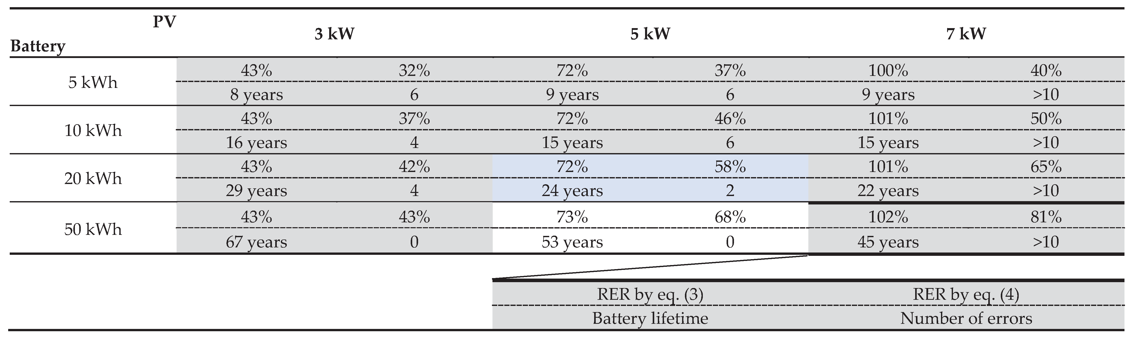
Table 6 summarizes the simulation results for all combinations of battery and solar panel capacities. For each configuration, the upper-left value represents the RER calculated using Equation (3), the upper-right value using Equation (4), the lower-left value indicates battery lifetime in years, and the lower-right value shows the number of annual voltage excursions.
Relative to the grid configuration (20 kWh battery and 5 kW solar panel), reducing the battery capacity to 10 kWh results in an RER below 50% (Equation (4)), a shortened battery lifetime of 15 years, and six voltage excursions per year—indicating reduced performance and compromised grid stability.
Similarly, reducing the solar panel output to 3 kW lowers both RER values below 50%, and leads to four voltage excursions annually.
Conversely, increasing the solar panel output to 7 kW yields an RER exceeding 100% (Equation (3)), indicating that annual generation surpasses consumption and grid export exceeds imports. Although an RER exceeding 100% is not necessarily problematic in itself, it implies that during high-generation periods—particularly in spring—frequent curtailment of PV output would be required to prevent abnormal rises in baseline voltage.
Increasing battery capacity to 50 kWh improves the RER to 68% (Equation (4)) and extends battery lifetime to 53 years. However, this far exceeds the typical lifetime of solar panels and other electronic components (approximately 20 years), resulting in system imbalance and substantially higher costs.
Therefore, the configuration examined in the previous section—20 kWh battery and 5 kW solar panel—can be considered optimal in terms of performance, grid stability, and overall system balance.
8. Conclusions
This study examined the configuration and characteristics of a DC microgrid designed for residential deployment, with the aim of realizing an eco-friendly lifestyle based on local production and consumption of solar-generated renewable energy. To ensure resilience against disasters and enable open, democratic management by local residents, we proposed a novel DC microgrid architecture based on autonomous decentralized cooperative control and a battery-integrated baseline.
In this configuration, the batteries directly connected to the grid baseline fulfill the essential functions of grid forming and maintaining. As a result, individual power devices—such as generators and loads—only need to monitor the voltage of the baseline to which they are connected. By autonomously regulating their power exchange with the baseline to avoid destabilizing the grid, control complexity is significantly reduced.
To realize autonomous decentralized cooperative control, each device must operate independently, without interference from neighboring devices. This requires a weakly coupled grid structure, where electrical coupling between devices is sufficiently limited. We demonstrated that this can be achieved by ensuring that the CR time constant—determined by the dynamic capacitance of distributed batteries and the conductor resistance of the baseline—is much larger than the control time constant τ of each device. Consequently, the influence of neighboring devices on a given sensing point is relatively slow and minor, preserving control independence.
A DC microgrid model comprising four typical residential houses was constructed in MATLAB/Simulink, and its behavior was analyzed over one year under realistic conditions in a Japanese city. The results showed that equipping each household with a 5 kW solar panel and a 20 kWh battery enables stable grid operation and sustainable living with a renewable energy ratio exceeding 50%. Using lithium iron phosphate batteries with a cycle life of approximately 3,000 cycles, a service life of around 25 years can be expected—comparable to that of solar panels and other electronic components—resulting in a well-balanced and durable system.
Furthermore, our results indicate that home EV charging can impose a substantial load on small-scale residential microgrids. Therefore, it is best to perform charging late at night when electricity consumption is at its lowest. In addition, if there are multiple charging facilities within the grid, care may need to be taken to avoid overlapping charging times between them as much as possible.
Funding
This research was funded by the JST OPERA Prog. (Grant Number JPMJOP1852).
Data Availability Statement
The original contributions presented in this study are included in the article. Further inquiries can be directed to the corresponding author.
Acknowledgments
The author would like to extend a special thanks to Liu Ke, who was a student in the author’s laboratory. Part of the content of this paper is based on the research conducted as part of her thesis under the guidance of the author. Additionally, through the JST OPERA project, the author had many valuable discussions with K. Iwatsuki and T. Otsuji. The author would like to express deep gratitude to them once again.
Conflicts of Interest
The author declares no conflicts of interest. The funders had no role in the design of this study; in the collection, analyses, or interpretation of data; in the writing of the manuscript; or in the decision to publish the results.
Abbreviations
The following abbreviations are used in this manuscript:
| AC | Alternative current |
| CV cable | Cross-linked polyethylene insulated Vinyl sheath cable |
| DC | Direct current |
| EMS | Energy management system |
| EV | Electric Vehicle |
| MPPT | Maximum power-point tracking |
| OSI | Open systems interconnection |
| PV | photovoltaic |
| RES | Renewable energy source |
| SoC | State of charge |
| SQ | square millimeters (mm2) |
References
- Xie, B.; Tian, X.; Kong, L.; Chen, W. The Vulnerability of the Power Grid Structure: A System Analysis Based on Complex Network Theory. Sensors 2021, 21, 7097. [CrossRef]
- Cetinay, H.; Devriendt, K.; Van Mieghem, P. Nodal vulnerability to targeted attacks in power grids. Appl. Netw. Sci. 2018, 3, 1–19. [CrossRef]
- Dias, J.; Montanari, A.N.; Macau, E.E.N. Power-grid vulnerability and its relation with network structure. Chaos: Interdiscip. J. Nonlinear Sci. 2023, 33, 033122. [CrossRef]
- Zahraoui, Y.; Korõtko, T.; Rosin, A.; Mekhilef, S.; Seyedmahmoudian, M.; Stojcevski, A.; Alhamrouni, I. AI Applications to Enhance Resilience in Power Systems and Microgrids—A Review. Sustainability 2024, 16, 4959. [CrossRef]
- Zhou, Y.; Zhao, Y.; Ma, Z.; Chen, L. Resilience analysis and improvement strategy of microgrid system considering new energy connection. PLOS ONE 2024, 19, e0301910. [CrossRef]
- Gao, Q.; Jiang, Y.; Peng, K.; Liu, L. A Virtual Inertia Method for Stability Control of DC Distribution Systems with Parallel Converters. Energies 2022, 15, 8581. [CrossRef]
- Samanta, S.; Mishra, J.P.; Roy, B.K. Virtual DC machine: an inertia emulation and control technique for a bidirectional DC–DC converter in a DC microgrid. IET Electr. Power Appl. 2018, 12, 874–884. [CrossRef]
- Zhou, D.; Chen, S.; Wang, H.; Guan, M.; Zhou, L.; Wu, J.; Hu, Y. Autonomous Cooperative Control for Hybrid AC/DC Microgrids Considering Multi-Energy Complementarity. Front. Energy Res. 2021, 9. [CrossRef]
- Nair, R.P.; Ponnusamy, K. Modeling and Simulation of Autonomous DC Microgrid with Variable Droop Controller. Appl. Sci. 2025, 15, 5080. [CrossRef]
- Yamada, H. Autonomous Decentralized Cooperative Control DC Microgrids Realized by Directly Connecting Batteries to the Baseline. Electronics 2025, 14, 1356. [CrossRef]
- Available online: https://en.wikipedia.org/wiki/OSI_model.
- Khan, M.Y.A.; Liu, H.; Yang, Z.; Wang, J.; Zhang, Y. Hierarchical control of microgrid: a comprehensive study. Electr. Eng. 2025, 1–32. [CrossRef]
- Liu, J.; Zhuan, X.; Shang, L.; Su, S.; Xie, Q. The Hierarchical Structure and Control Signal Transmission of Microgrid Hierarchical Control: A Review. IET Power Electron. 2025, 18. [CrossRef]
- Liu, K.; Yamada, H.; Iwatsuki, K.; Otsuji, T. Experimental Verification and Simulation Analysis of a Battery Directly Connected DC-Microgrid System. Int. J. Electr. Electron. Eng. Telecommun. 2023, 12. [CrossRef]
- Available online: https://www.jma.go.jp/jma/indexe.html.
- Available online: https://www.kankyo.metro.tokyo.lg.jp/documents/d/kankyo/home-energy-files-syouhidoukouzittaityousa26honpen_3 (In Japanese).
- Available online: https://www.env.go.jp/content/900449221.pdf in Japanese, Cited from p.41, Figure 4.5.
- Takusagawa, T.; Uchida, H.; Fujii, H.; Yoshimura, S. Evaluation of the influence of electric vehicles’ charging demand on power system. 2018, The 32nd Annual Conference of the Japanese Society for Artificial Intelligence, 4D2-OS-18c-03 in Japanese. [. [CrossRef]
- Rostami, H.; Valio, J.; Tynjälä, P.; Lassi, U.; Suominen, P. Life Cycle of LiFePO4 Batteries: Production, Recycling, and Market Trends. Chemphyschem 2024, 25, e202400459. [CrossRef]
- Sun, S.; Guan, T.; Cheng, X.; Zuo, P.; Gao, Y.; Du, C.; Yin, G. Accelerated aging and degradation mechanism of LiFePO4/graphite batteries cycled at high discharge rates. RSC Adv. 2018, 8, 25695–25703. [CrossRef]
- Botejara-Antúnez, M.; Prieto-Fernández, A.; González-Domínguez, J.; Sánchez-Barroso, G.; García-Sanz-Calcedo, J. Life cycle assessment of a LiFePO4 cylindrical battery. Environ. Sci. Pollut. Res. 2024, 31, 57242–57258. [CrossRef]
Figure 1.
Conventional DC baseline (a) and battery-integrated DC baseline (b).
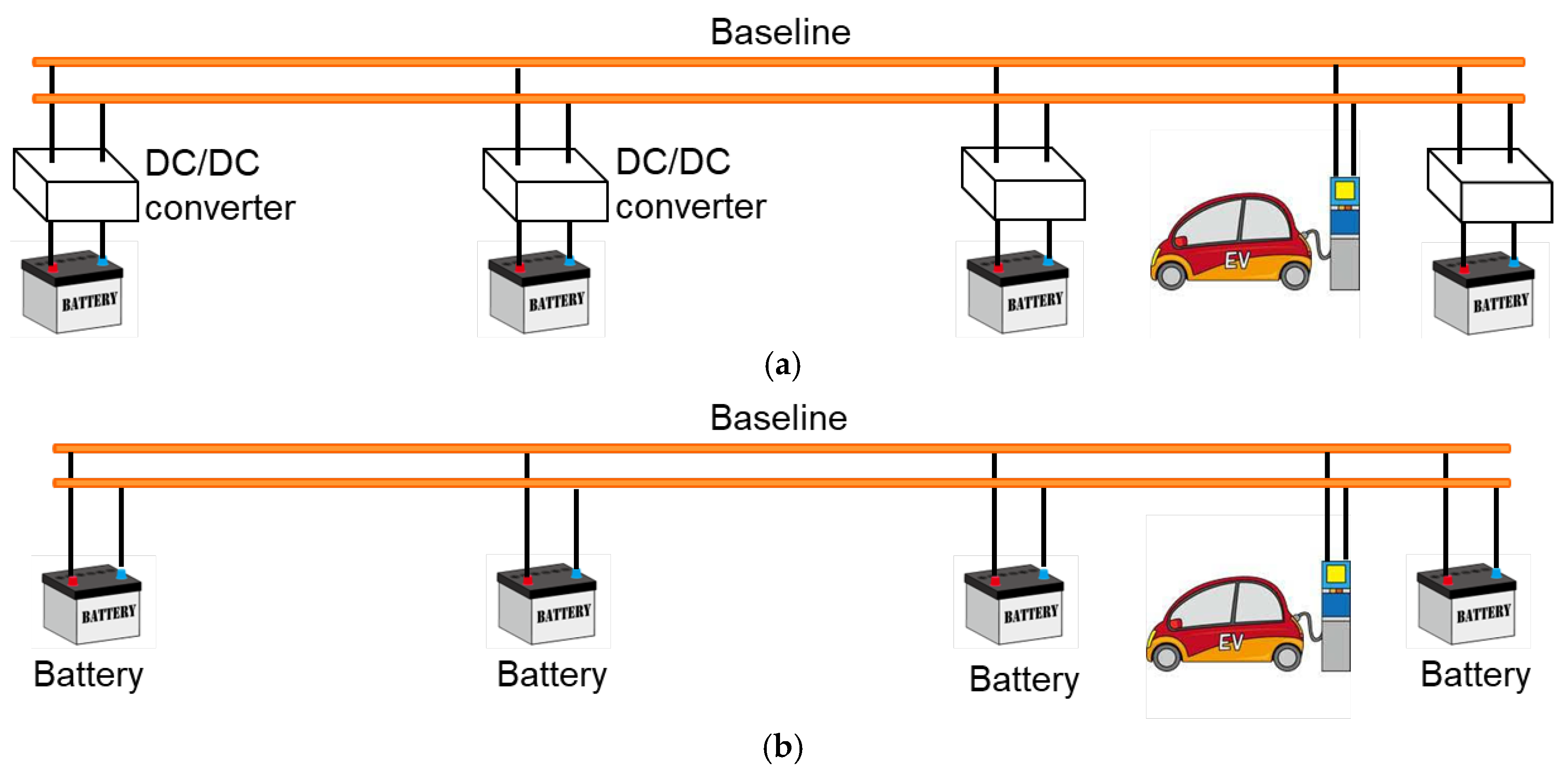
Figure 2.
Comparison of the roles of each device between conventional DC grid (a) and battery-integrated DC grid (b).
Figure 2.
Comparison of the roles of each device between conventional DC grid (a) and battery-integrated DC grid (b).
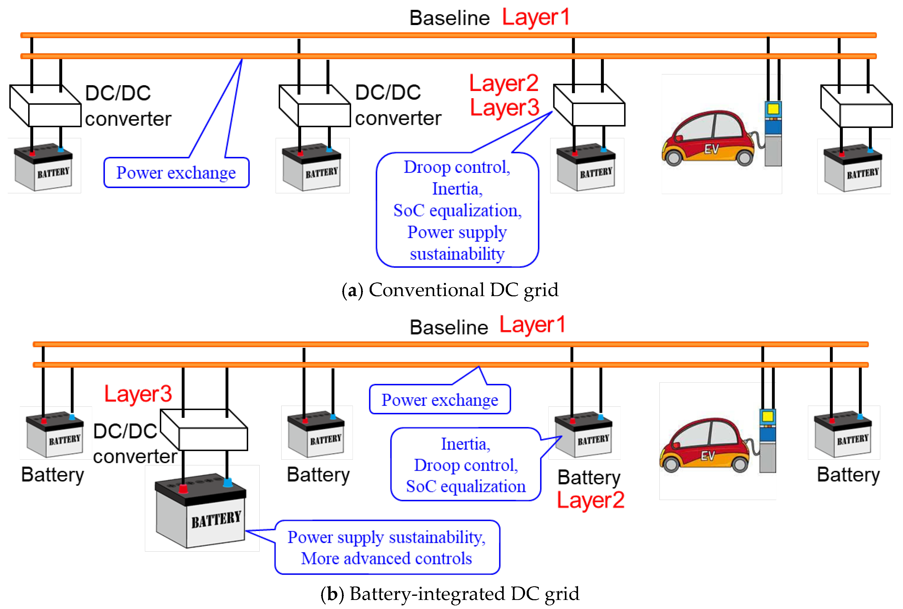
Figure 3.
Electrical inertia on the baseline; (a) 6.6 kV distribution grid line; (b) 400 V DC microgrid baseline.
Figure 3.
Electrical inertia on the baseline; (a) 6.6 kV distribution grid line; (b) 400 V DC microgrid baseline.
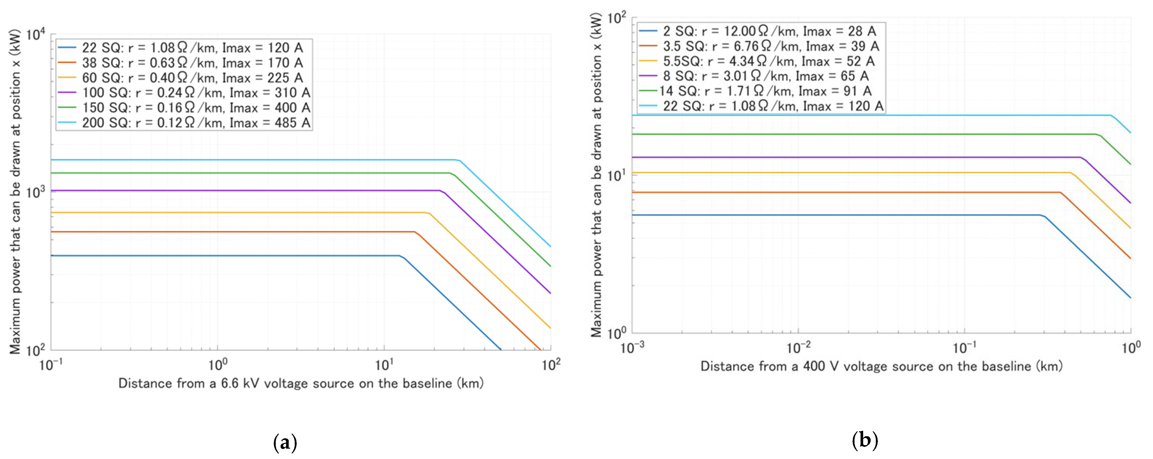
Figure 4.
The need for local control to ensure the independence of each device control.
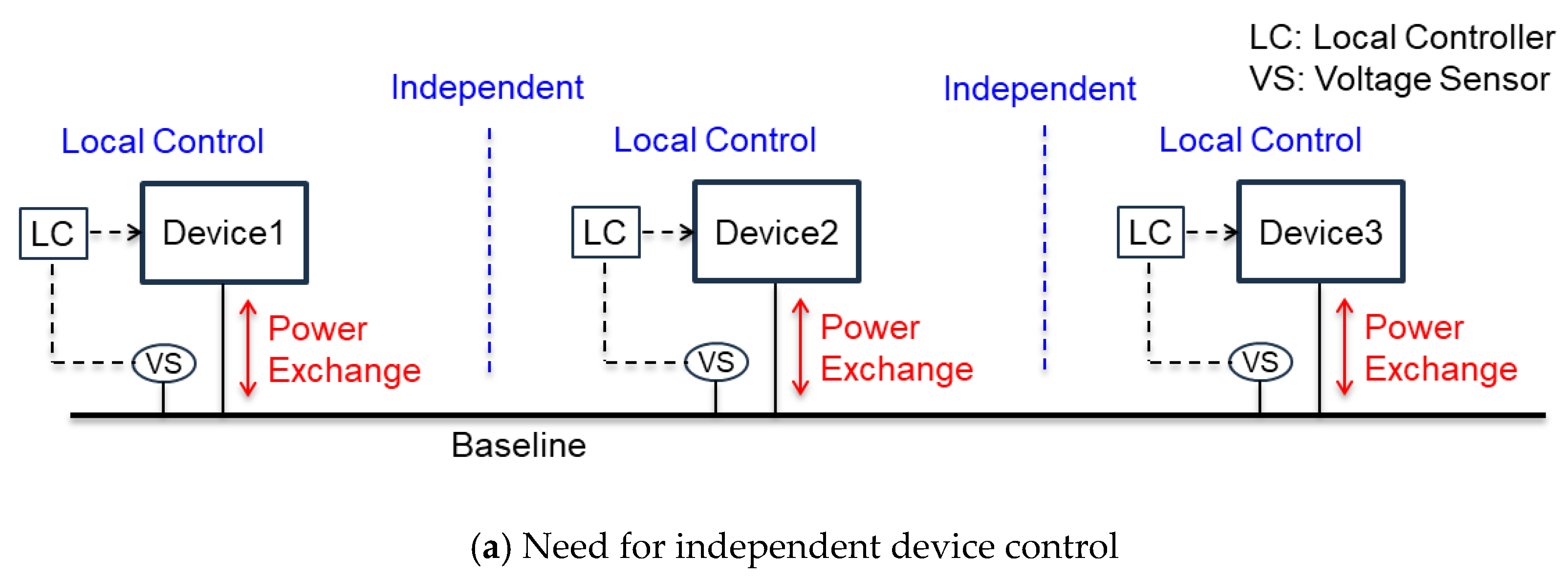
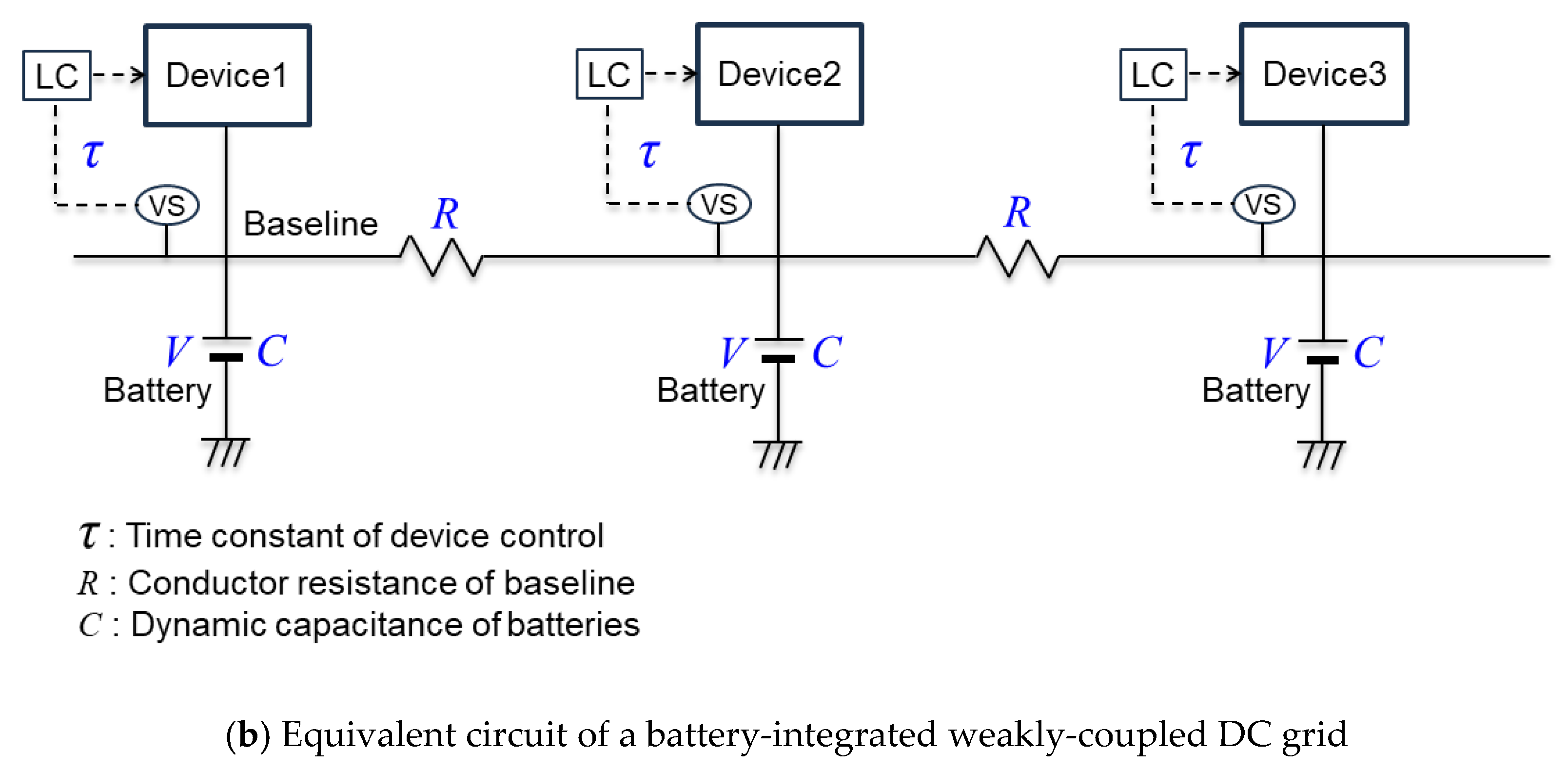
Figure 5.
Daily electricity consumption pattern of a typical Japanese house.
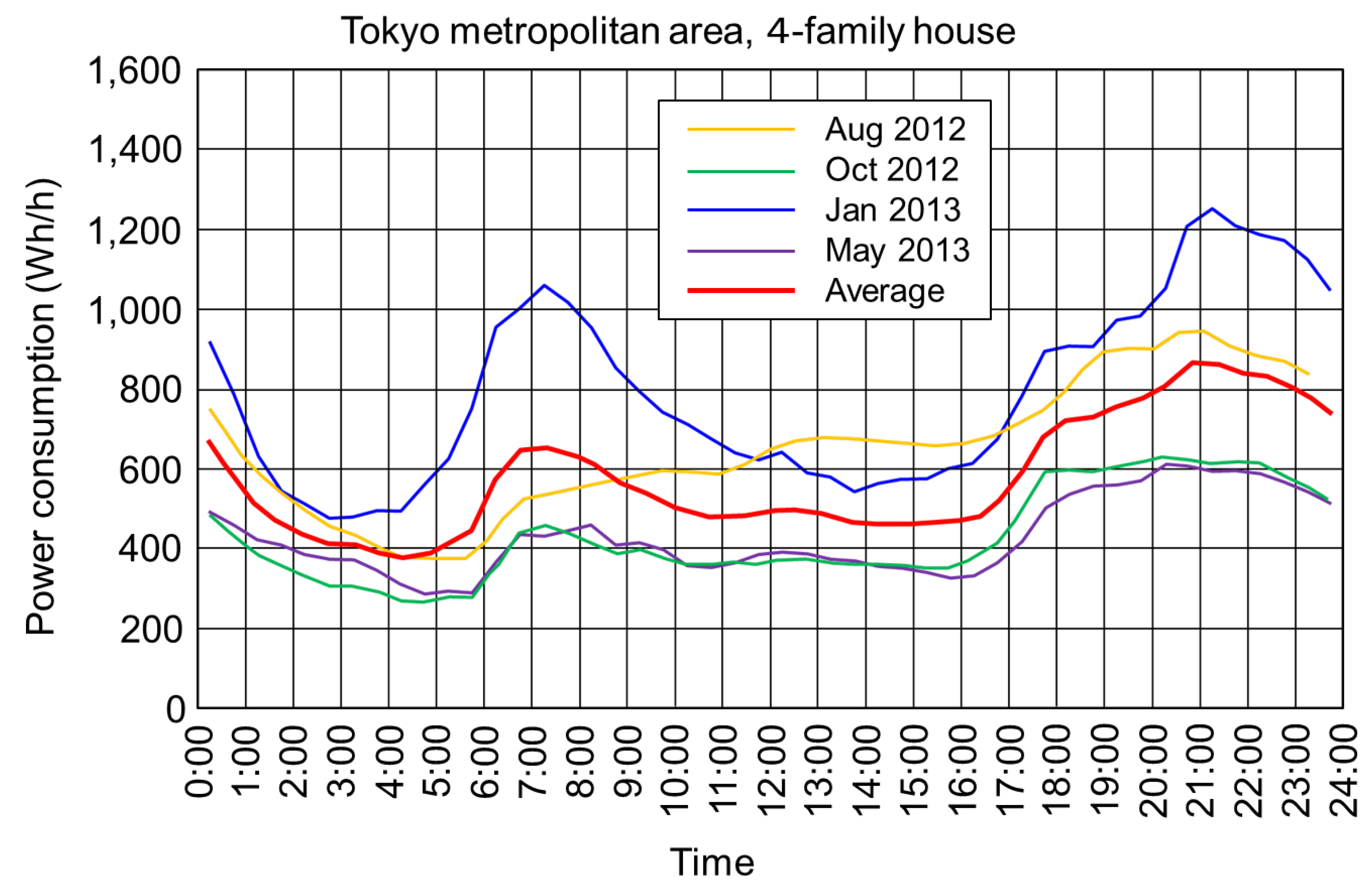
Figure 6.
Simulation model of a four houses DC microgrid.
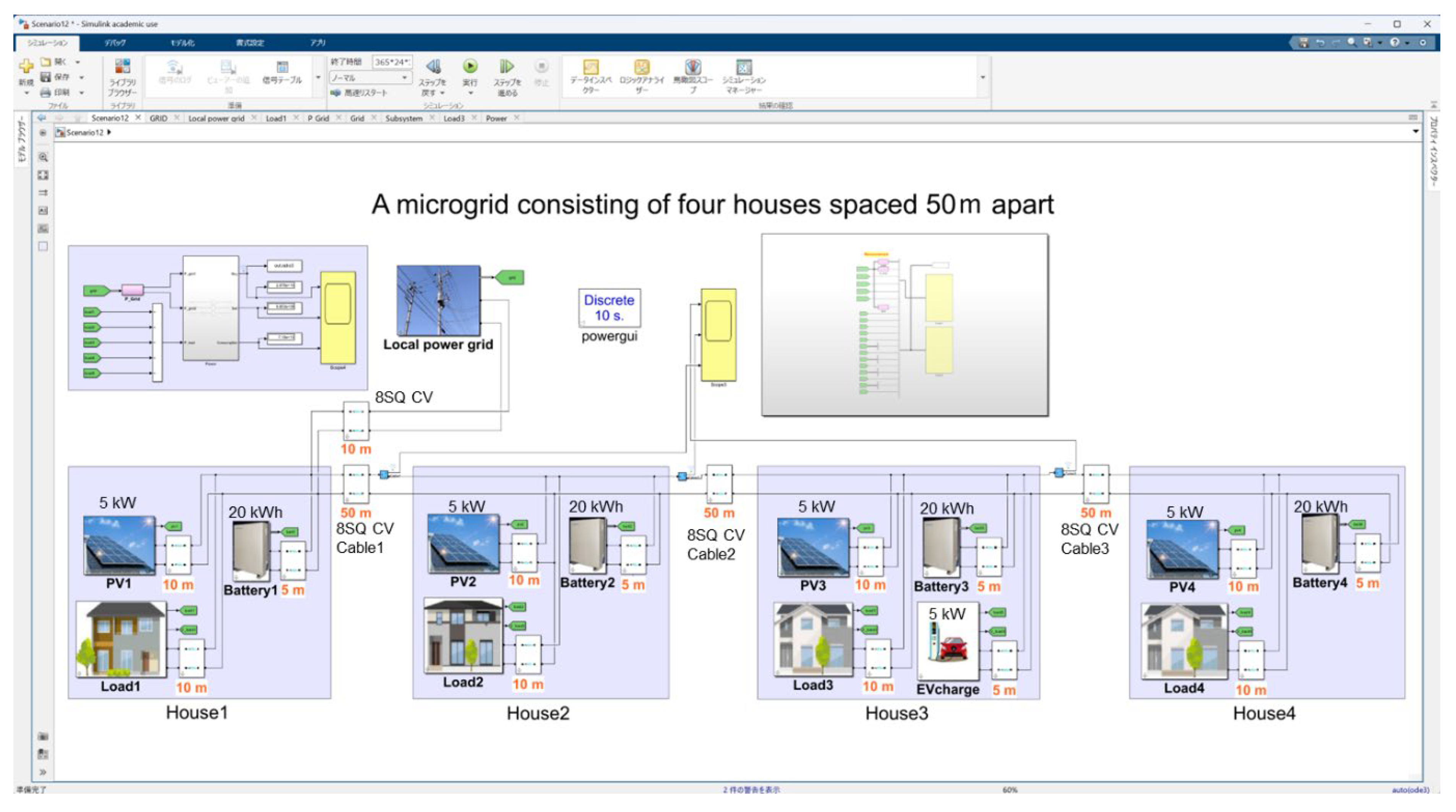
Figure 7.
Annual variation and a detailed view of the January monthly variation in the power generated by the solar panel installed on each house.
Figure 7.
Annual variation and a detailed view of the January monthly variation in the power generated by the solar panel installed on each house.
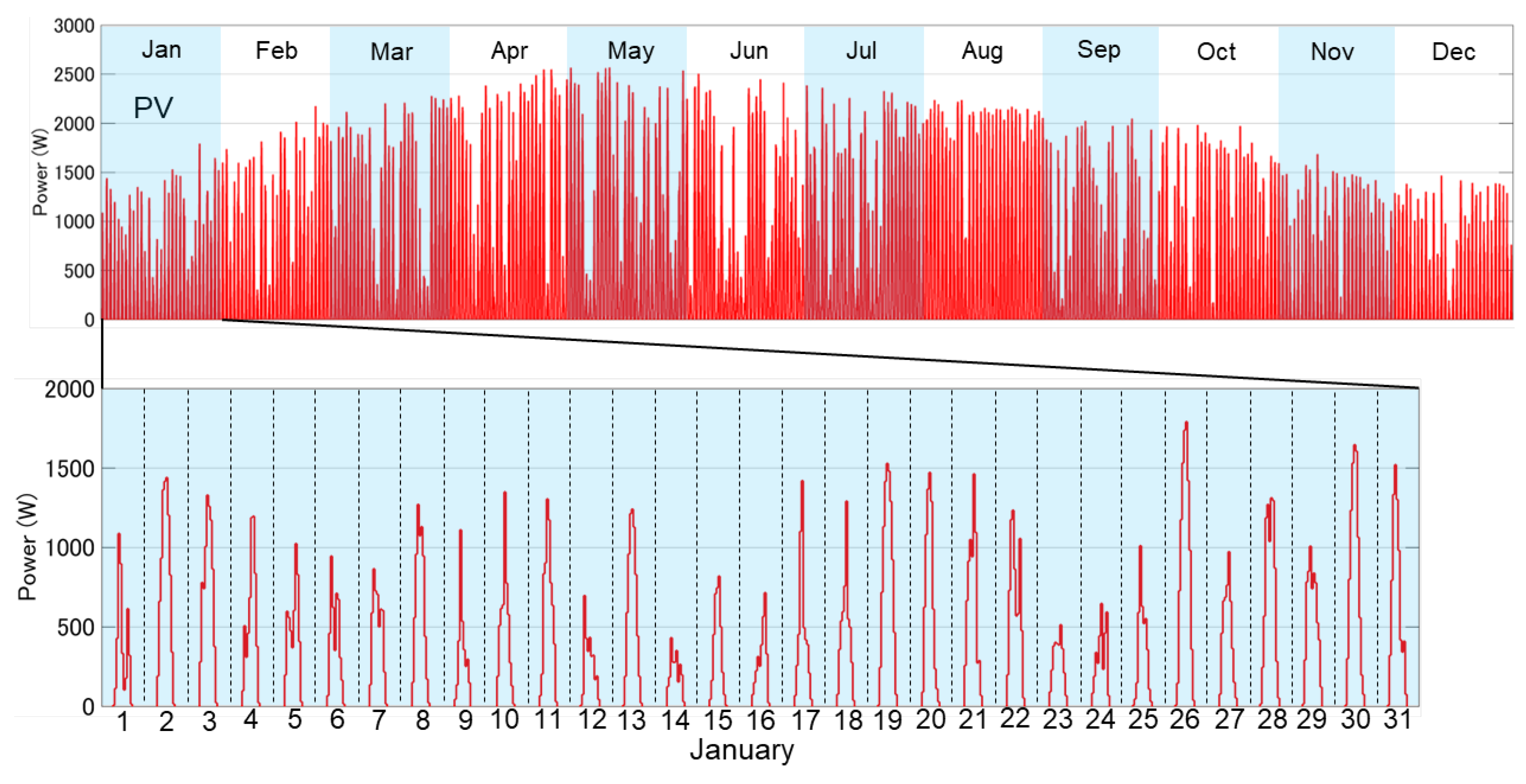
Figure 8.
Annual variation in electricity consumption across the four households, along with a detailed view of the January variation for House4.
Figure 8.
Annual variation in electricity consumption across the four households, along with a detailed view of the January variation for House4.
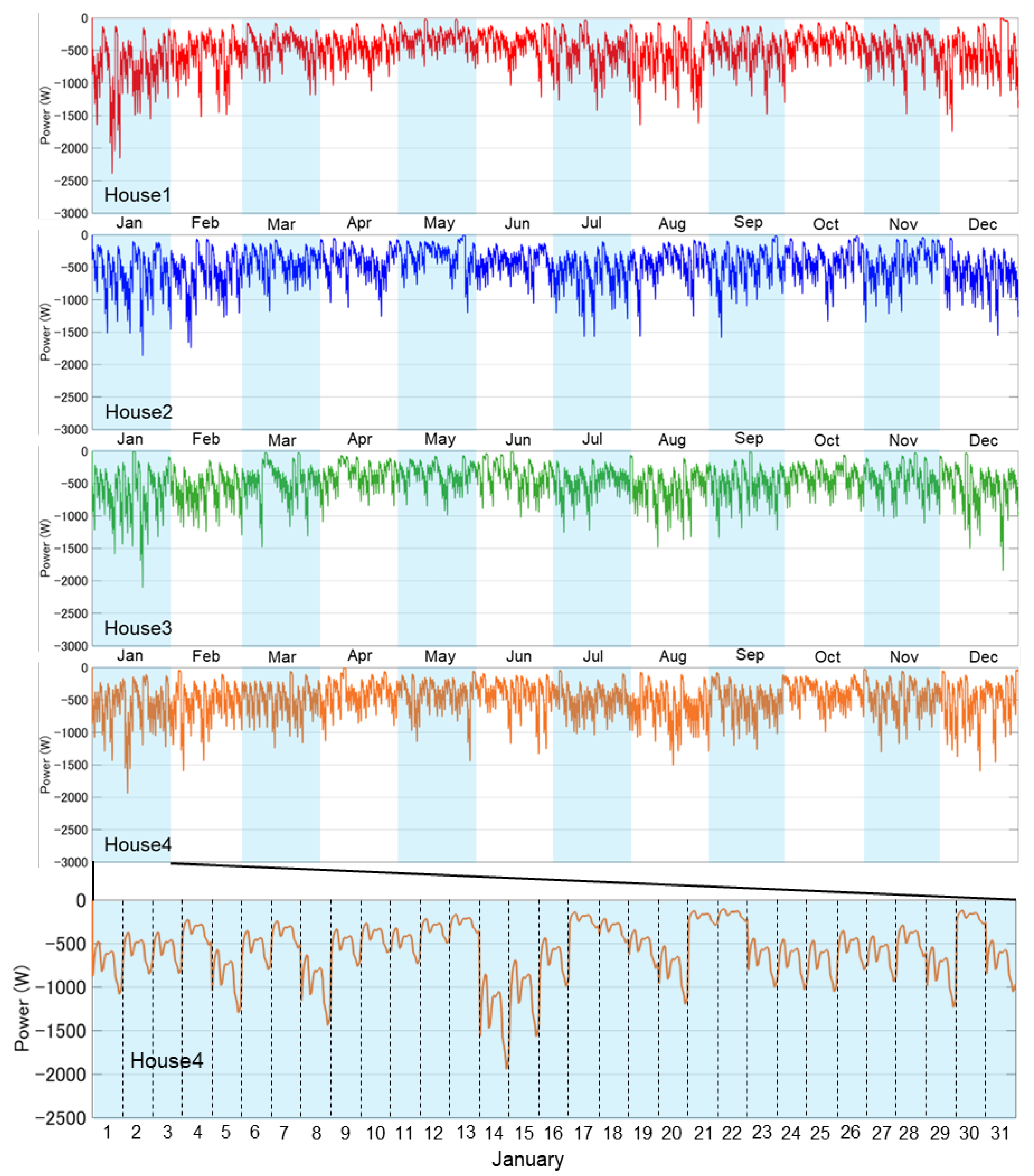
Figure 9.
Annual variation in baseline voltage at each household’s connection point.
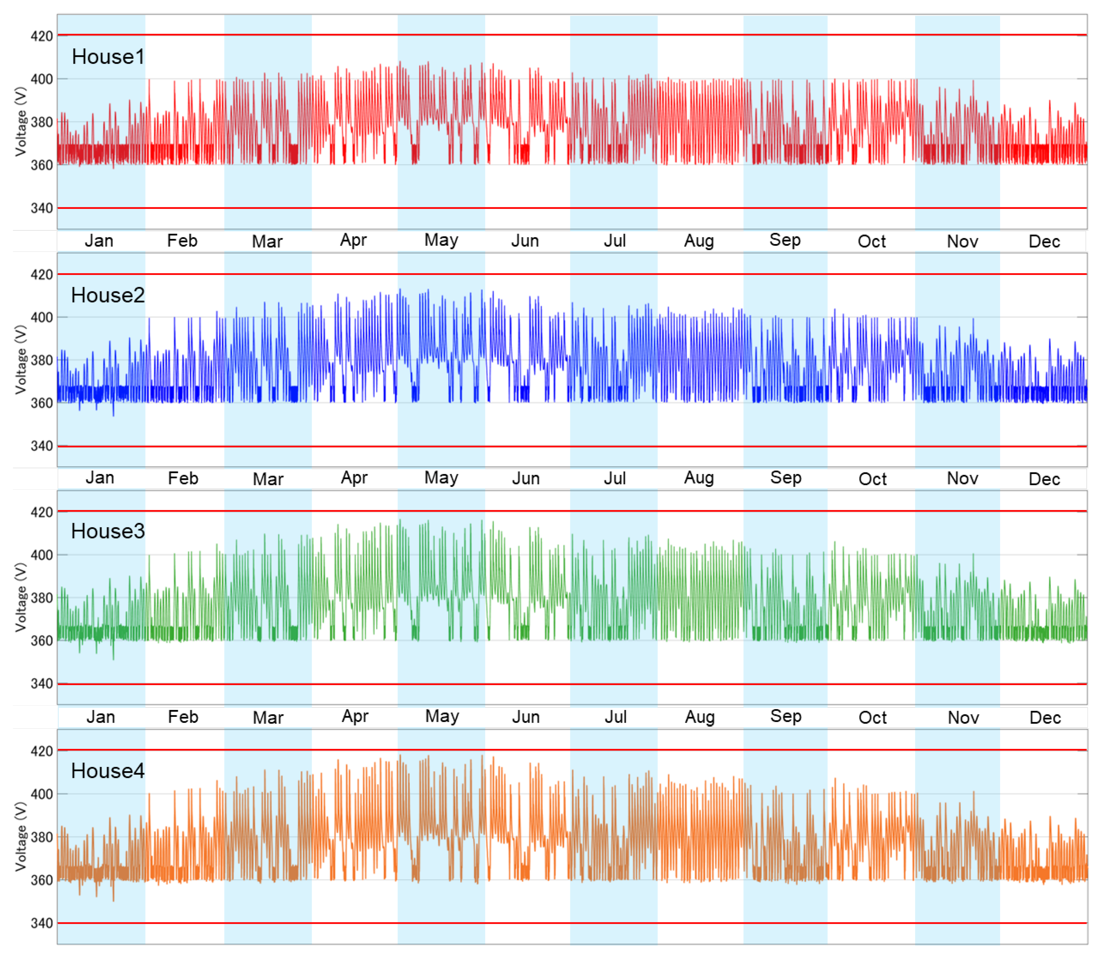
Figure 10.
Annual variation of charging and discharging power of the batteries installed in each house.
Figure 10.
Annual variation of charging and discharging power of the batteries installed in each house.
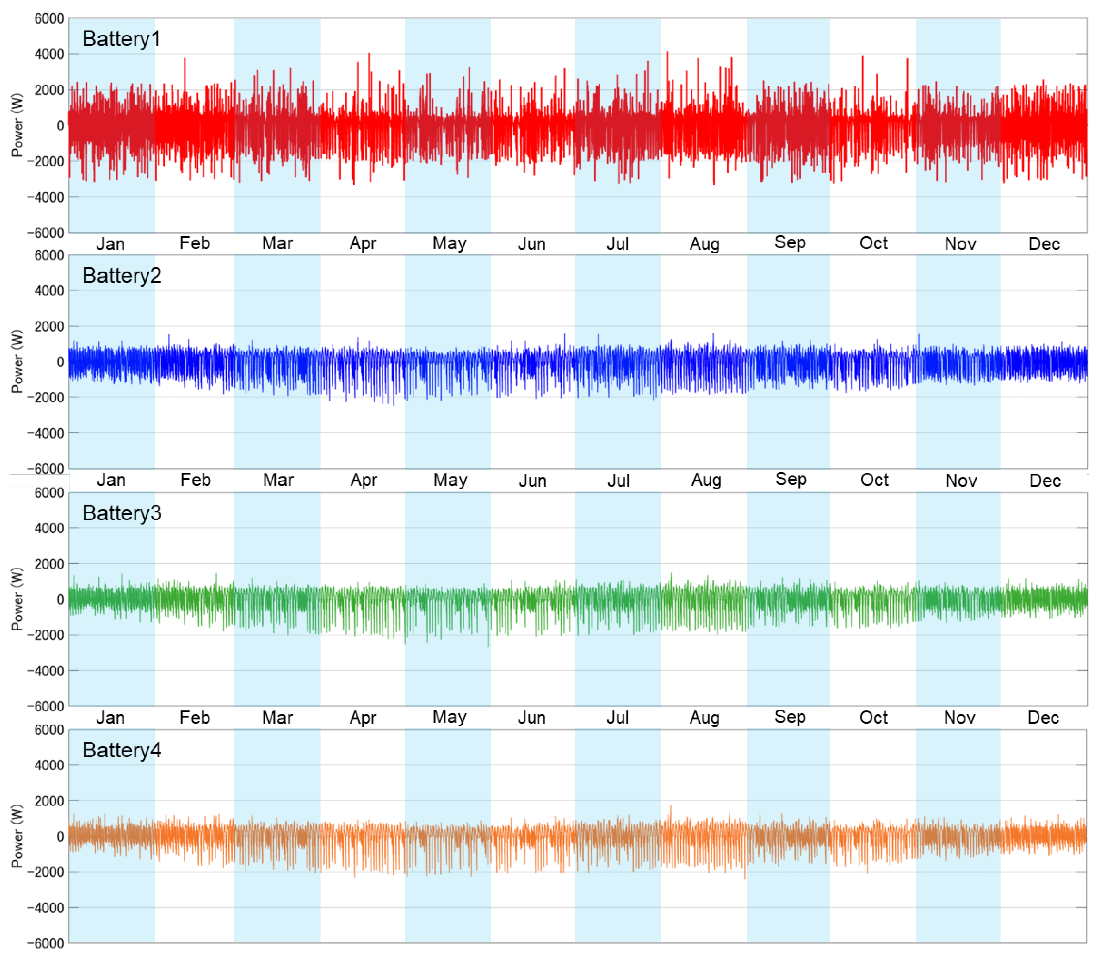
Figure 11.
Cumulative charge/discharge current over time.
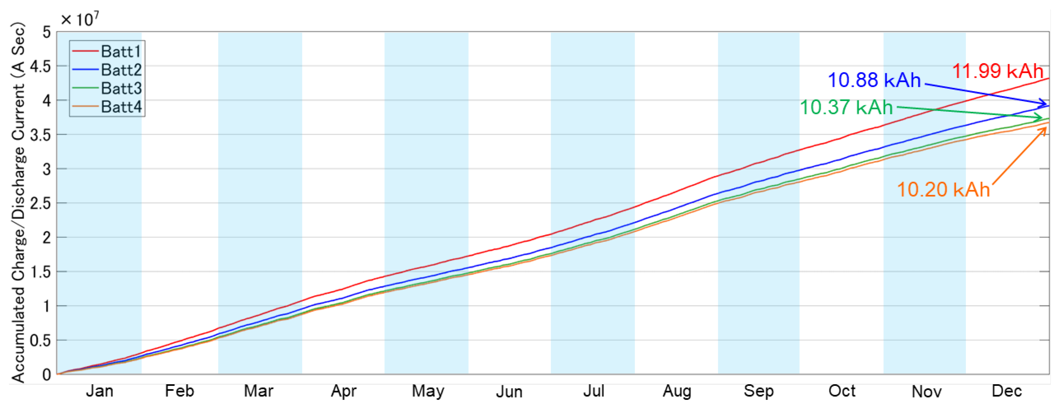
Figure 12.
Current flowing through the baseline cables connecting the houses.
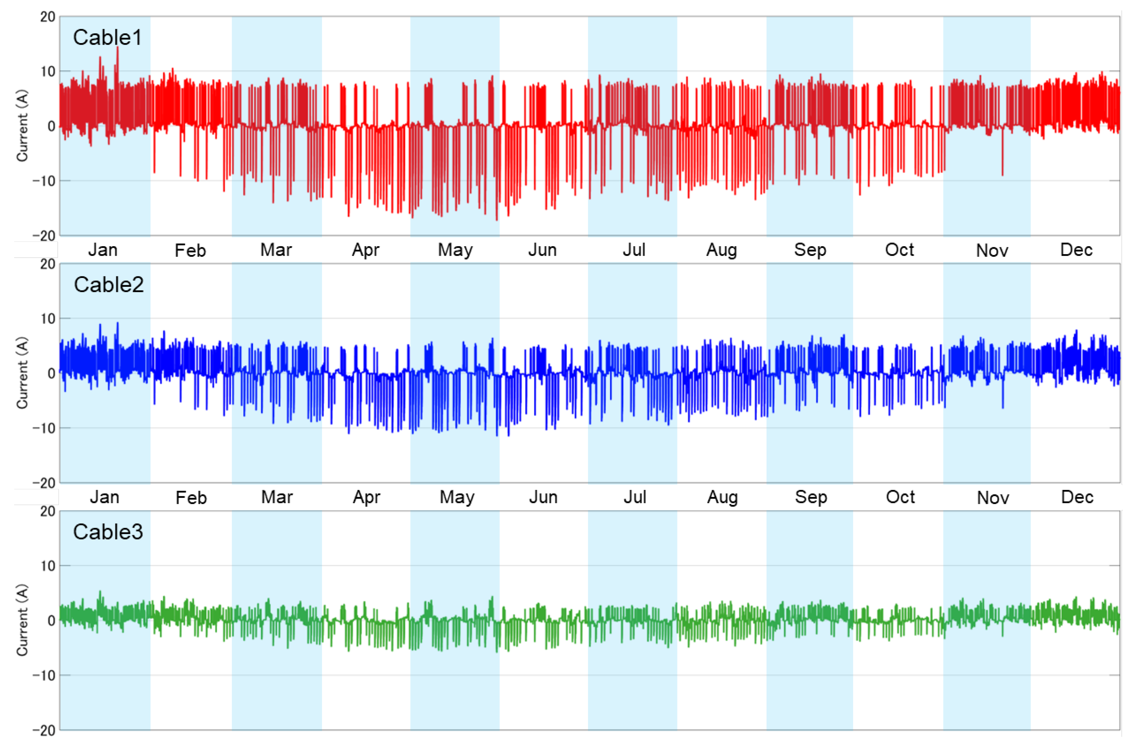
Figure 13.
Power exchange with the utility grid.
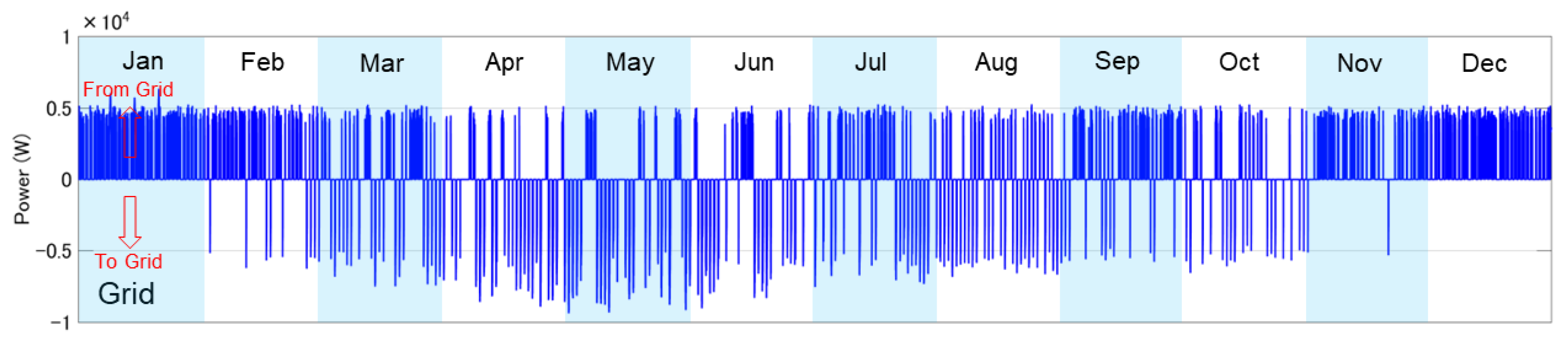
Figure 14.
Cumulative power consumption, grid import, and grid export for the entire microgrid.
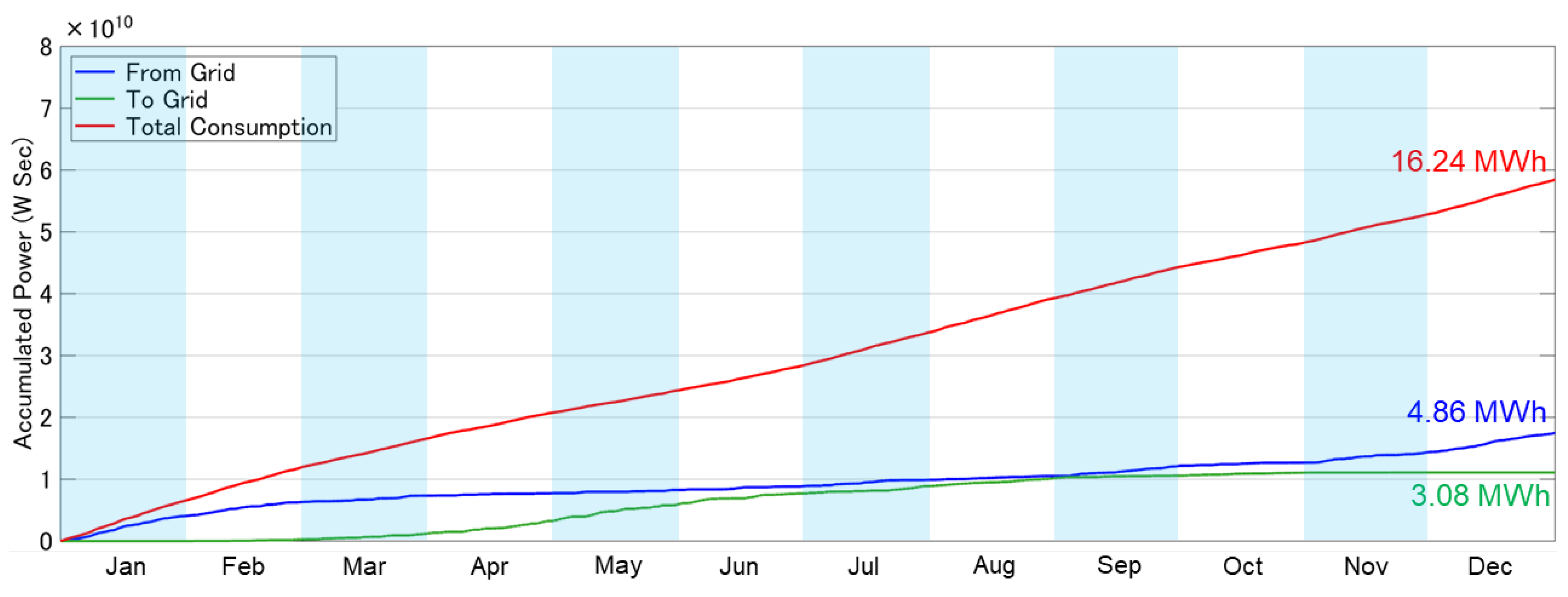
Figure 15.
Annual variation in baseline voltage at each household’s connection point.
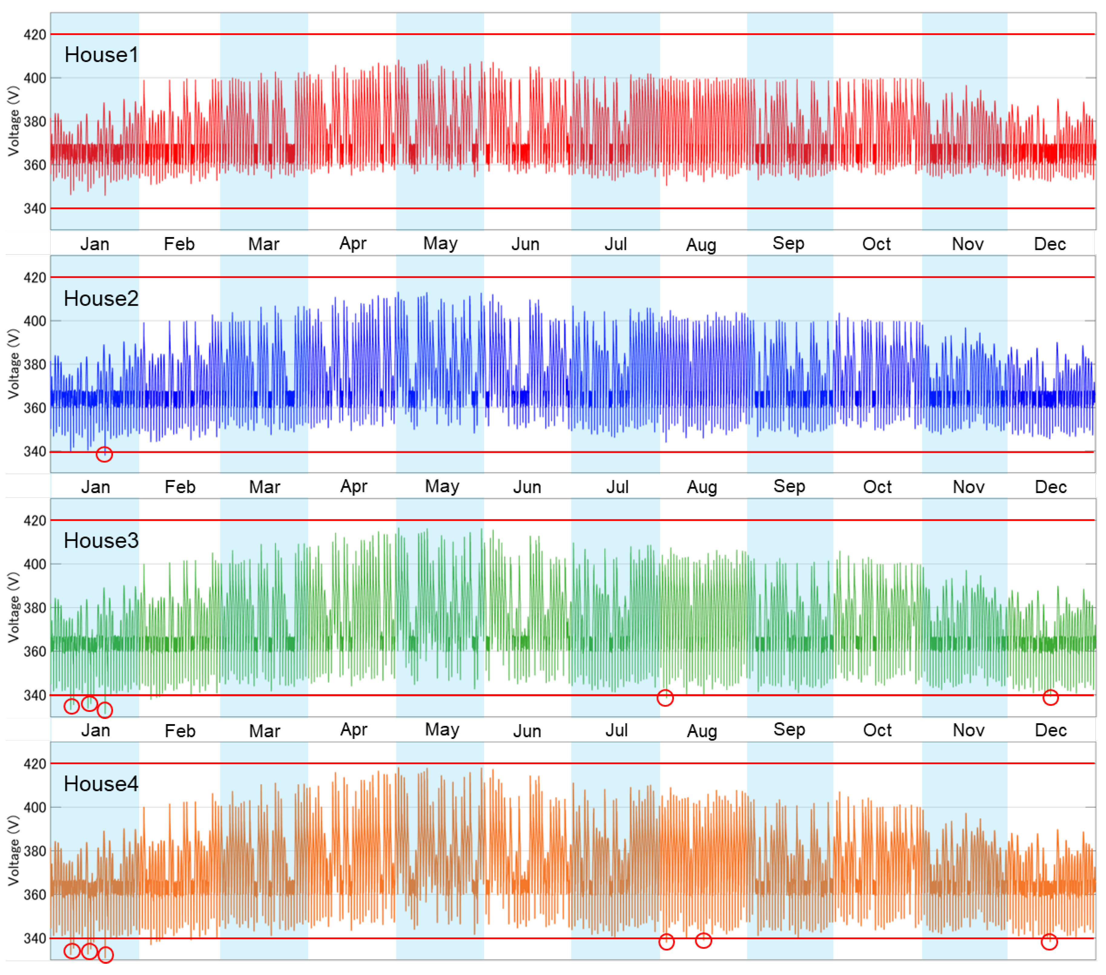
Figure 16.
Annual variation in baseline voltage at each household’s connection point when EV charging times are shifted to between 2:00 and 4:00 AM.
Figure 16.
Annual variation in baseline voltage at each household’s connection point when EV charging times are shifted to between 2:00 and 4:00 AM.
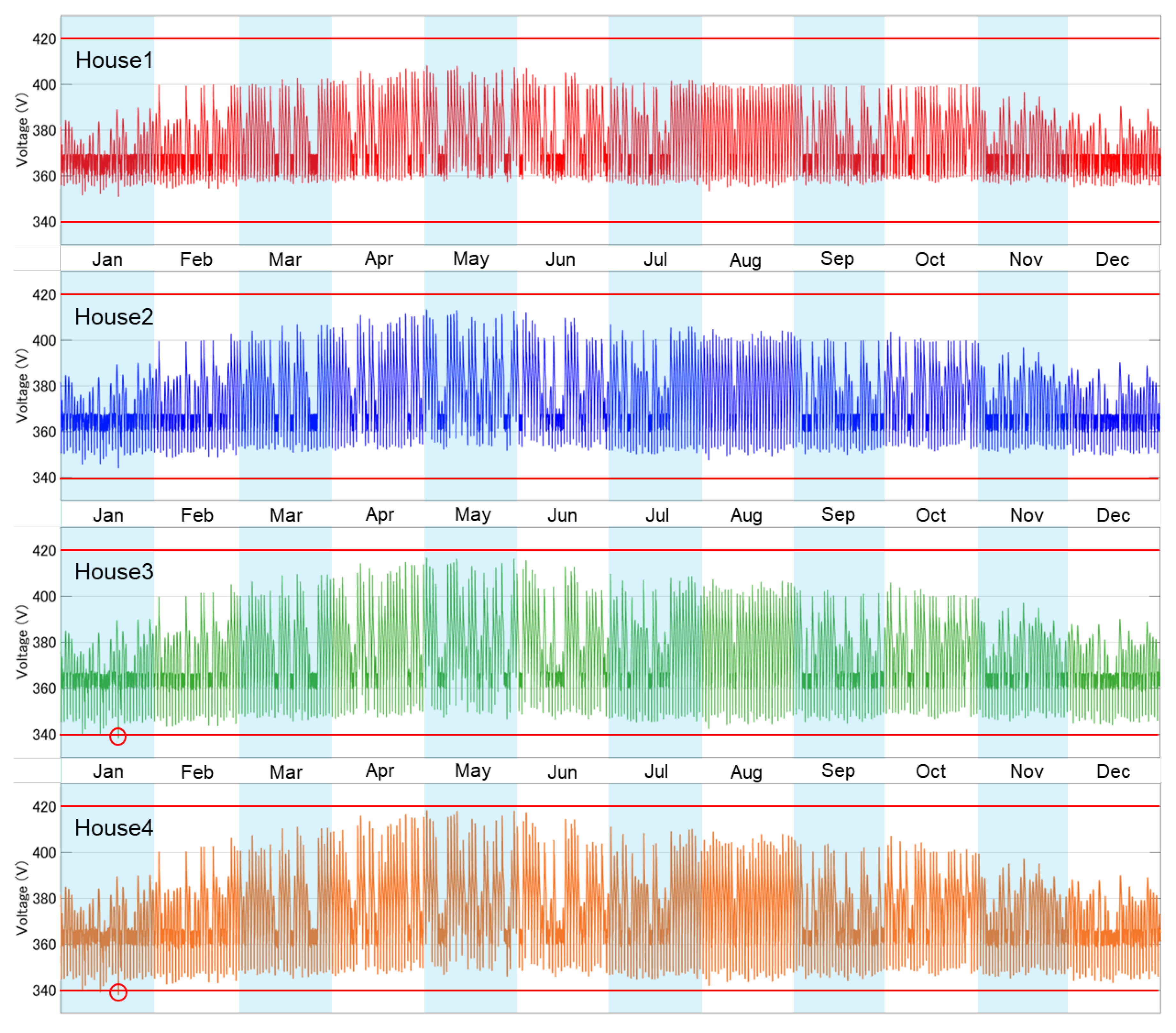
Figure 17.
Cumulative charge/discharge current over time.
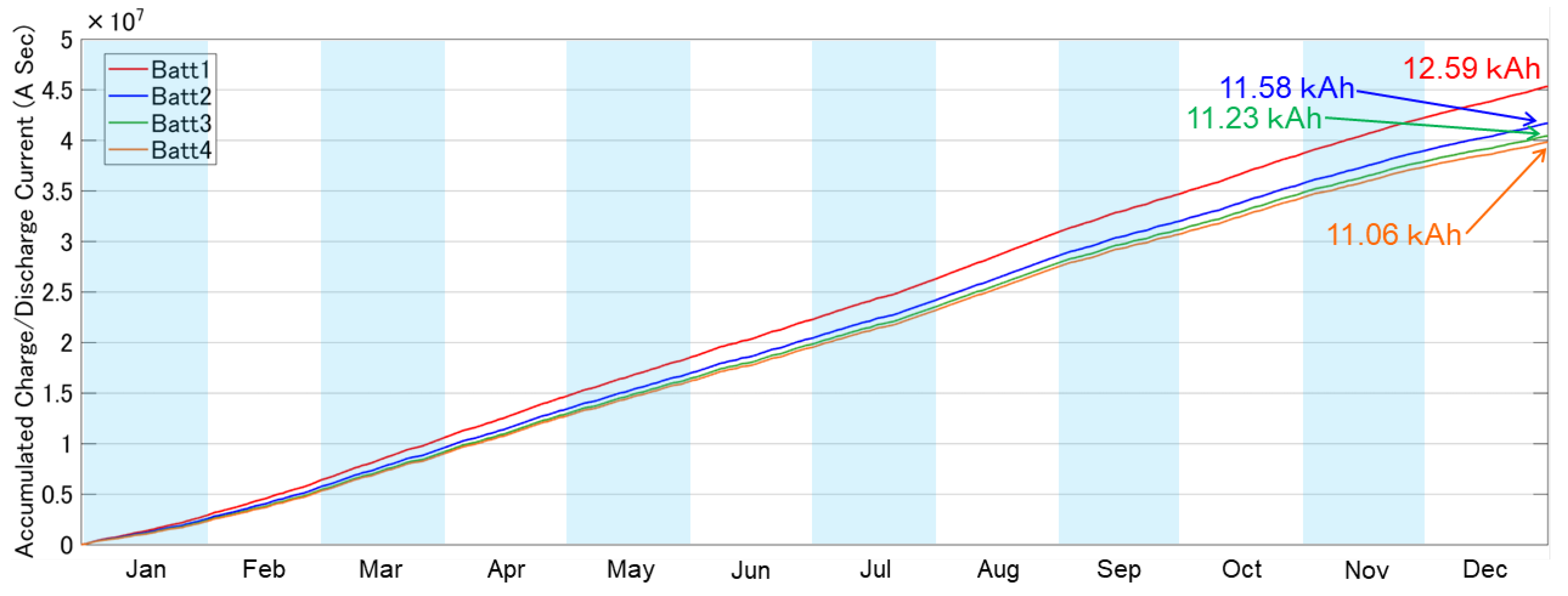
Figure 18.
Cumulative energy consumption, grid import, and grid export for the entire microgrid.
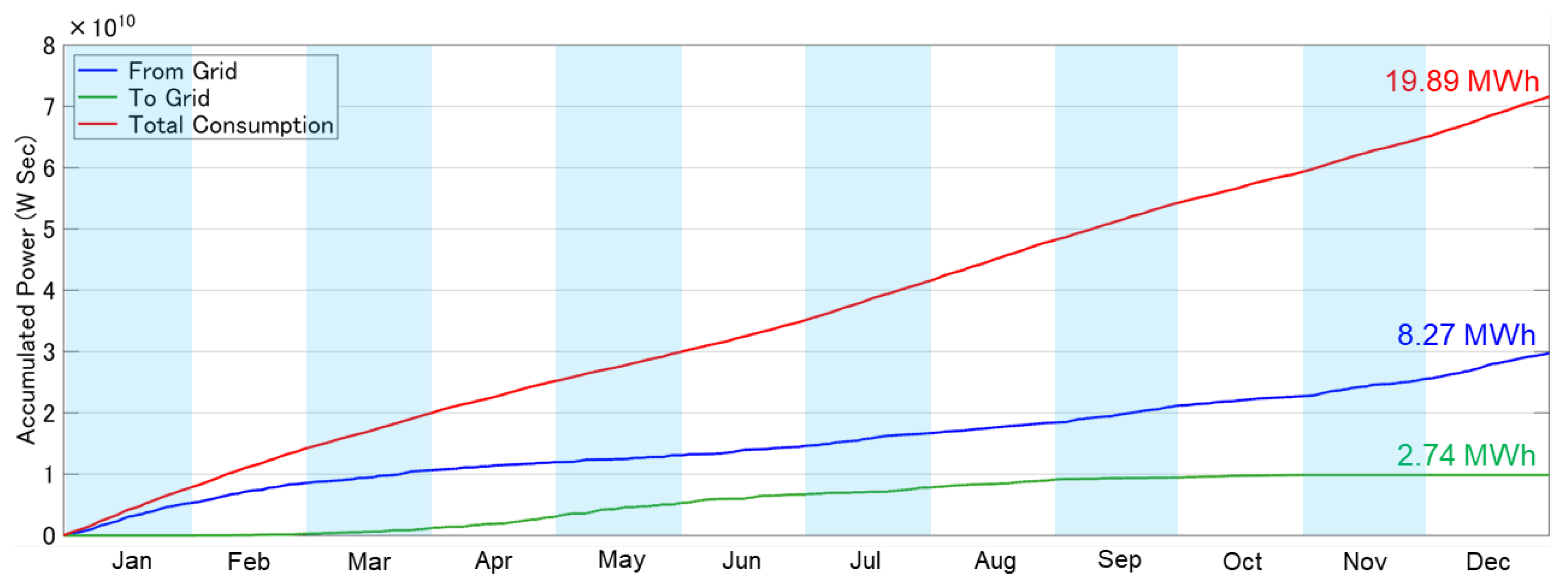

Table 1.
Comparison of existing power grids and microgrids.
| Existing power grid | Microgrid | |
| Concept of power usage | Transporting electricity over long distances | Local production and consumption |
| Power source | Centralized | Distributed |
| Type of power | High-voltage AC | Low-voltage DC, (AC) |
| Grid topology | River-flow (Tree) | Bus, Ring, Mesh, etc. |
| Power flow | Unidirectional | Bidirectional |
| Control method | Centralized control | Decentralized control |
| Resilience | Low | High |
| IntroducingRES* | Difficult | Easy |
| Major consumer | Industrial, Residential | Residential |
| Issue | Maintenance and management of grid | Cost reduction of storage batteries |
* Renewable energy sources.
Table 2.
Layering of grid functions.
| Layer No | Layer Name | Function | Methods |
| 4 | Application layer | Various applications that utilize grids | EMS*, Power trading |
| 3 | Power exchange layer | Power exchange between grid and devices, Connection to other grids, (droop control) |
Control of DC/DC converters |
| 2 | Grid forming layer | Basic functions for forming and maintaining stable grid (Electrical inertia, droop control, Equalizing power distribution, Ground fault, short circuit and lightning strike protection) |
Control of DC/DC converters, Batteries directly connected to baseline (AC or DC, Baseline voltage) |
| 1 | Physical layer | Physical medium that enables power exchange between power devices (Power line) |
CV cable, etc. (2-core or 3-core, Grounding method) |
* Energy management system.
Table 3.
Comparison of responsible devices between conventional DC grids and battery-integrated DC grids.
Table 3.
Comparison of responsible devices between conventional DC grids and battery-integrated DC grids.
| Grid function |
Conventional DC microgrid |
Battery-integrated DC microgrid |
| Power applications | Control of DC/DC converters (EMS*, Electricity trading, EV charging) |
Control of DC/DC converters (EMS*, Electricity trading, EV charging) |
| Power exchange between grid and devices | DC/DC converters (Maintaining power supply, Power exchange) |
DC/DC converters (Maintaining power supply, Power exchange) |
| Forming,maintaining and stabilizing grid | DC/DC Converters (Electrical inertia, Droop control, SoC equalization) |
Distributed batteries directly connected to the baseline (Electrical inertia, Droop control, SoC equalization) |
| DC-baseline | Power cable | Power cable |
* Energy management system.
Table 4.
Average monthly electricity consumption of a typical Japanese household [kWh/month].
| Jan | Feb | Mar | Apr | May | Jun | Jul | Aug | Sep | Oct | Nov | Dec |
| 429 | 372 | 312 | 270 | 260 | 260 | 331 | 403 | 324 | 257 | 297 | 394 |
Table 5.
Parameters of the simulation model.
| Solar panel | Battery | EV charging infrastructure | |||
| Rated output power (kW) | Installation efficiency (%) | Capacity (kWh) | Initial SoC (%) | ||
| House1 | 5 | 50 | 20 | 50 | none |
| House2 | 5 | 50 | 20 | 50 | none |
| House3 | 5 | 50 | 20 | 50 | 5 kW |
| House4 | 5 | 50 | 20 | 50 | none |
Table 6.
Summary of the impact of system capacity on RER, battery lifetime and grid stability.
 |
Disclaimer/Publisher’s Note: The statements, opinions and data contained in all publications are solely those of the individual author(s) and contributor(s) and not of MDPI and/or the editor(s). MDPI and/or the editor(s) disclaim responsibility for any injury to people or property resulting from any ideas, methods, instructions or products referred to in the content. |
© 2025 by the authors. Licensee MDPI, Basel, Switzerland. This article is an open access article distributed under the terms and conditions of the Creative Commons Attribution (CC BY) license (http://creativecommons.org/licenses/by/4.0/).
Copyright: This open access article is published under a Creative Commons CC BY 4.0 license, which permit the free download, distribution, and reuse, provided that the author and preprint are cited in any reuse.


