
Submitted:
22 August 2025
Posted:
25 August 2025
You are already at the latest version
Abstract
This paper proposes a method to predict the backscattering of multilayer rectangular and circular slabs with arbitrary thickness, dielectric constant, and conductivity over all frequency ranges. The radar cross section is defined as a function of the internal field generated on each individual layer. The internal electric field is derived analytically through boundary conditions at each layer, representing the amplitude, phase, and polarization of the dispersed wave in the distant field. The multi-layer estimation of radar cross section is validated using results from a single-layer slab and experimental data from diverse literature. The model can additionally be employed to simulate the radar cross section of various landscapes and natural environments, where distinct re-gions such as vegetation, desert, or clouds are characterized by differing permittivity and thickness to derive the radar cross section. This study aims to introduce a novel adaptive adaptation for human detection by assessing the thickness of pierced walls. To ascertain the penetrated wall thicknesses, the frequency response of the wall must first be established. The calculation of frequency response employs two models: a single antenna model and a dual antenna model. The frequency response equations for each model are employed to examine the calculated received signal, establishing a correlation between reflections and wall thickness. The backscattering signals are simulated for a single antenna model, including signals arriving from various angles. For the twin an-tenna model, received signals are simulated for scenarios involving transmission via multilayer structures, walls, and individuals.
Keywords:
wall imaging
; multi-layered structures
; radar scattering area
; inner electric field
1. Introduction
Dielectric layers are essential for modeling natural phenomena, including plant leaves and ice crystals in high-altitude clouds [1]. In contrast to the completely conducting slab [2,3], an exact solution for scattering from a dielectric layer remains undiscovered. Reported approximations pertain to both high and low frequency extremes [2,3,4,5], whereas numerical methods have been established for mid-frequencies [1,6,7,8,9]; however, a singular, comprehensive estimate applicable across all frequencies is absent. Le Vine [10] developed an approximation for the radar cross section (RCS) of electrically thin, single-layered structures, when the thickness is significantly less than the wavelength.
The importance of scattering of electromagnetic waves in the explanation of natural phenomena was first appreciated by Lord Rayleigh when he was investigating the problem of scattering by a perfectly conducting sphere. During the past few decades, research in electromagnetic scattering by a variety of objects and targets assumed added importance because of its direct relevance to all radar applications and, in particular, to radars used for military and space exploration where the main objectives are to locate, identify and classify various objects. Typical radar accomplishes these objectives by processing the received signals, which usually consists of desired signals scattered by targets and the undesired noise of clutter signals, the former containing the information characteristic of the targets. The received scattered signal power is directly proportional to the scattering or RCS of the targets, and hence the importance of RCS of the objects.
During the early years of radar any acceptable methodology for calculation and measurement of RCS of objects was considered adequate for radar engineers. Literature on the analysis, computation, and measurement of RCS of variety of objects is extensive and still growing [11,12,13]. With better understanding of the electromagnetic scattering phenomena it is natural that consideration is now being given to deliberate control of the RCS of objects for various applications. For example, with rapid advancement in missile and space technology attention increasingly is being directed toward disguising the presence of a flying object to unfriendly radar by reducing its RCS.
Apart from the estimation and measurement of RCS and its control requires in the preceding applications, the RCS study finds important use in remote sensing and inverse scattering or imaging. Although in the latter two areas some inversion algorithms generally are required, the input data are the complex scattered fields derived either from experiment or a suitable analytical model. Because modern theoretical research on RCS depends largely on the available computer power, role of development of computer storage and speed on the capability of solving electromagnetic problems is very important in general. Innovative methods of fast processing of large matrices, parallel processing in computers and concepts of neural networks may help the situation.
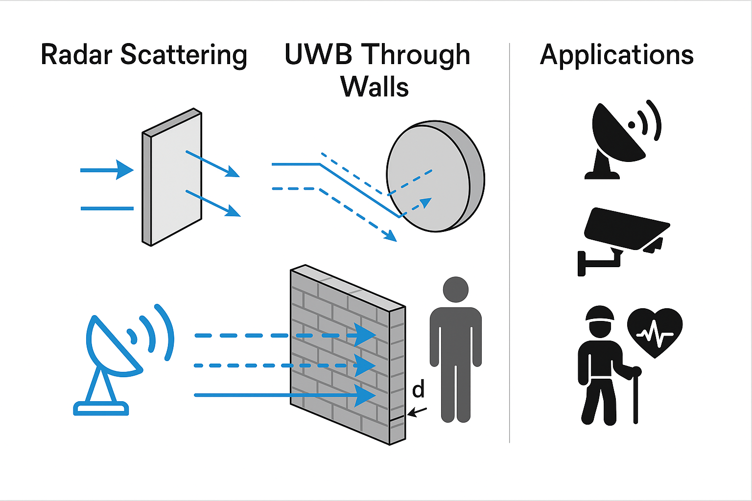
Numerous scenarios exist in which entering a room or structure is deemed perilous, necessitating the inspection of the interior from outside through walls. An illustration encompasses the monitoring of individuals in perilous settings. Search and rescue personnel would significantly benefit from through-the-wall imaging during time-sensitive incidents such as fire rescues or structural collapses. The principal aims of this project are to comprehend the propagation of ultra-wideband (UWB) radar waves, to model UWB radar signal propagation, and to develop mathematical algorithms for ascertaining wall thickness, thereby enabling the accurate representation of any building without prior knowledge of the building material [14,15,16,17,18,19,20]. In radar systems for human detection, the second most critical design consideration, following bandwidth, is the selection of the pulse repetition frequency. It influences the unequivocal range of the radar, which should be approximately 30 meters at a minimum, and the duration of individual signal measurements, which should be roughly five times shorter than the normal respiratory cycle. To maintain an adequately high power budget for the system, a substantial average number is preferable.
The first basic concept is that frequency is meaningless if UWB systems use electromagnetic pulses, rather than short wave-packets. Pulse repetition frequency (PRF) could be declared, but this is not a correct figure of electromagnetic spectrum occupation. PRF is typically in the range from 1 to 50 MHz. Furthermore the pulse repetition period is often modulated to carry information or coding. A more precise frequency description of UWB emission could be given by the Fourier transform of the pulse. One performance measure of a radio in applications like communication, locating, tracking, and radar, is the channel capacity for a given bandwidth and signaling format. By virtue of the huge bandwidths inherent to UWB systems, huge channel capacities could be achieved in principle (given sufficient signal to noise ratio (SNR)) without invoking higher order modulations that need very high SNR to operate.
In situations necessitating stealth, certain UWB formats, particularly those based on pulses, can be effectively disguised as a minor increase in background noise to any receiver oblivious to the signal’s intricate pattern. The dielectric constant and loss tangent of the material under examination can be derived from the intricate insertion transfer function. The selection of the analytical technique depends on the efficacy of time gating implementation. In some instances, multiple reflections within the slab diminish swiftly, resulting in single-pass and multiple-pass approaches producing virtually identical outcomes.
The confidence in the given result is bolstered when time-domain and frequency-domain measurements are congruent, due to the involvement of various equipment, calibrations, and processes. The frequency-domain approach offers two advantages: it enables characterization across a broader frequency spectrum through the use of multi-band filters, and it does not necessitate external synchronization. Both input and output are processed centrally, thereby minimizing synchronization errors. Conversely, the time-domain technique provides superior resolution and an increased number of data points. Analysis of data indicates that time-domain measurements utilizing brief pulses demonstrate reduced variability compared to frequency domain results across the relevant frequency spectrum.
2. Theory and Problem Statement
The transmitter (or source), usually located at a large distance from the target illuminates target, which starts acting as a secondary radiator to produce scattered fields at the receiver or observation point, also usually located at a large distance from the target. Monostatic or backscattering occurs when the transmitter and receiver are collocated, and bistatic scattering occurs when they are separated in space by an angle called bistatic angle.
A specific case of a single layer dielectric slab in order to get acquainted with the theory and terminology will be presented firstly. Then, how the general case of multilayered dielectric slab can be extended will be explained. Later, the theory of the multilayer case will be presented. Referring to the literature and using reflection coefficients obtained via recursion formulas, this study ends up with a better approximation for simulation purposes obtaining similar results with the experiments done using thin dielectric slabs. This multilayer approximation technique using a single layered slab is tested and then expanded to multilayered cases for drawing conclusion about the nature of radar cross section.
2.1. Electric field inside multi-layer slab
An electromagnetic wave of any kind of polarization can be decomposed into its orthogonal linearly polarized components. Those that have their electric field parallel to the interface are called horizontally polarized and H polarization (also referred to as parallel polarization). We have a transverse electromagnetic wave that is incident at some arbitrary angle θo upon a multi-layer dielectric slab of N layers. For each layer thickness di, permittivity εi and the loss tangent (tanδi) are arbitrary, the permeability is that of free space (μ0).
Figure 1.
Demonstration of electric fields of a multi-layered slab.
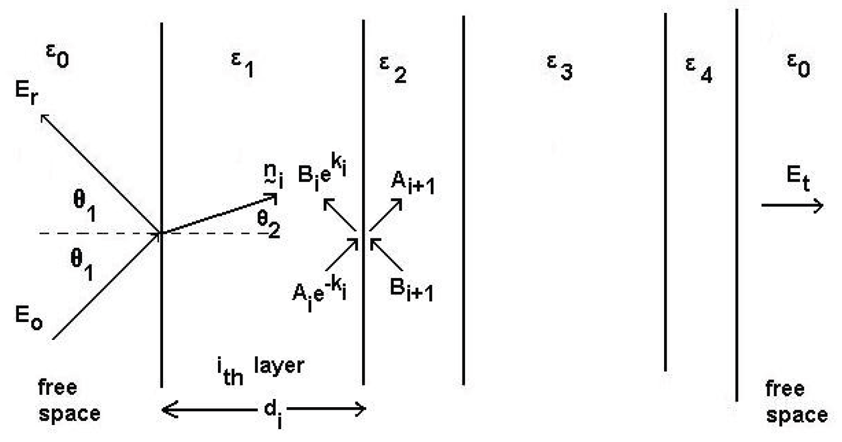
The diagram above outlines the concept for scattering from a multilayered slab. Let’s define the following scalar quantities; Ai: tangential electric field at the left interface of the ith layer, propagating from left to right Bi: tangential electric field at the left interface of the ith layer, propagating from right to left. Fi: tangential H at the left interface of the ith layer, moving from left to right Gi: tangential magnetic field at the left interface of the ith layer, propagating from right to left [11].
2.2. Perpendicular (vertical) polarized wave
Values for A_i and B_i can be derived from boundary conditions:
where
Reflection coefficient R is defined as the ratio of reflected Er to incident Eo field intensities in free space to the left of the first plane boundary. Transmission coefficient T is defined as the ratio of transmitted Et to incident Eo field intensities in free space to the left of the first plane boundary.
2.3. Parallel (horizontal) polarized wave
The identical derivation is conducted for perpendicularly polarized waves, with the coefficients Ai interchanged, yielding values for Fi and Gi based on boundary conditions.
where .
Reflection and transmission coefficient for parallel polarized waves are as follows:
Wavenumber can simply be expressed as .
is the complex propagation constant through the ith layer. Given that reflection and transmission coefficients are complex values, fundamental division cannot be executed; however:
3. Employing a Multi-Layer Model for Simulation
3.1. Simulating a single layered dielectric slab with a multi-layer model
The slab is presumed to possess a cross-sectional shape , a thickness T, and is composed of a material with a relative dielectric constant εr = εr’ + jεr’’. εr is presumed to remain constant throughout the slab, and the configuration of the slab S(r̄) is arbitrary. The objective is to ascertain the radar cross section of the slab in the context of backscatter (monostatic cross section). is delineated in relation to the scattered electric field polarized in the p̂ direction, resulting from an incident wave with polarization q̑ as follows:
Evaluating scattering amplitude in terms of internal electric field:
Here, denotes a unit vector originating from the coordinate center of the slab directed towards the observer, whereas Ro represents the distance from the slab’s center to the observer. where ,
if rectangular slab;
if circular slab;
adar (backscatter) cross section in terms of complex is:
Let’s calculate a function for for both vertical and horizontal polarization by evaluating the internal electric field in a multilayered slab. Since the second layer of the dielectric slab represents the internal field of interest and the first and third layers are regarded as free space, i=2 is utilized: internal polarization fields for v and h.
Observing that due to orientation of the angles
Using Taylor expansion for and using the first three terms, substituting value for C:
To obtain formulas for horizontal polarization, Ai is substituted by Fi, and Bi is substituted by Gi:
The shape function S is crucial for the determination of radar cross-section. The function is contingent upon the slab’s shape being either rectangular or circular. If the form is rectangular:
If shape is circular:
where J1 denotes Bessel function of first order.
Finally radar cross section is obtained using Equation (13):
3.2. Verification of simulation results
3.2.1. Case 1: Thin rectangular slab
Object: Single layered thin square dielectric slab, Incident Angle: -30 to 30 degrees
Thickness of dielectric slab: 1.06*10-4 m, εr= 2.272, Con = 1.67*10^-15 mho, Length of a side (Xo): 0.3048 m
The simulation result presented in Figure 2 for the single-layered thin square slab is consistent with Le Vine’s model outcomes under Case 1 conditions at 4 GHz [10]. In Figure 3, the results of the multilayer model are shown for Case 1 conditions at 4 GHz, illustrating both vertical and horizontal polarizations.
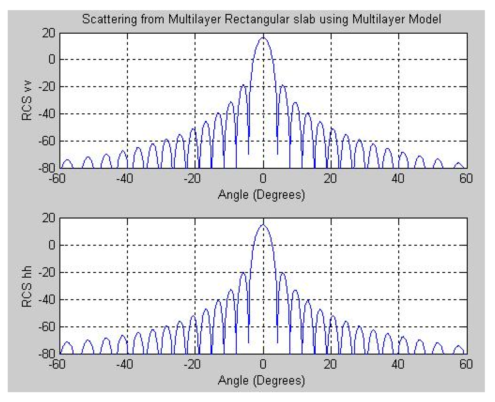
Figure 4 presents the results of Case 1 for both vertical and horizontal polarizations at 16 GHz. The experimental findings for Case 1 under horizontal polarization at 16 GHz, as reported in [10], are in clear agreement with the results shown in Figure 4. In Figure 5, the simulation outcomes of the multilayer model are provided.
3.2.2. Case 2: Thick Circular Slab
Object: Single layered thick circular dielectric slab, Incident Angle: -60 to 60 degrees
Thickness of dielectric slab: 0.05 m, εr= 11, Radius of a side (Xo): 0.2 m
Frequency: 9 GHz
Figure 6 and Figure 7 respectively illustrate the results for a single-layered and a multi-layered thick circular dielectric slab at 9 GHz, under both vertical and horizontal polarizations. The horizontal polarization results presented in Figure 6 exhibit clear consistency with the findings reported by Le Vine [10].
3.2.3. Case 3: Thin circular slab with complex permittivity
Object: Single layered circular dielectric slab, Incident Angle: -60 to 60 degrees
Thickness of dielectric slab: 0.0004 m, εr= 25+j11, Radius of a side (Xo): 0.2 m
Frequency: 5 GHz
Figure 8 and Figure 9 present the simulation results for a thin circular slab with complex permittivity at 5 GHz, corresponding to the single-layered and multilayered cases, respectively. The close similarity between the single-layered results and those reported by Le Vine [10] at 5 GHz serves to validate the accuracy of these simulations.
3.2.4. Case 4: Thick circular slab with complex permittivity
Object: Single layered circular dielectric slab, Incident Angle: -60 to 60 degrees
Thickness of dielectric slab: 0.005 m, εr= 25+j11, Radius of a side (Xo): 0.1 m
Frequency: 9 GHz
Figure 10 and Figure 11 depict the simulation results of a thick circular slab with complex permittivity at 9 GHz for both the single-layered and multilayered cases, under vertical and horizontal polarizations. The simulations of several dielectric slab configurations show that the proposed multilayer model can accurately anticipate how RCS will behave in diverse situations. The model closely matched both experimental results and Le Vine’s simulations at 4 GHz and 16 GHz for the thin rectangular slab. It effectively illustrated the impact of polarization on various aspects. It also showed a strong match with reference models for both thick and thin circular slabs, even when the permittivity was complicated. This consistency across variations in thickness, material properties, and frequency highlights the method’s reliability. The model’s results are quite similar to those of experiments or benchmark simulations, which further shows that it is accurate and useful for real-world radar scattering applications.
4. Radar Cross Section (RCS) of Multi-Layer Slab
Let’s consider a multi-layered rectangular structure shown below and obtain its RCS using the proposed method:
The model above has these parameters: Length of a side: 0.3048 m, Frequency: 4 GHz
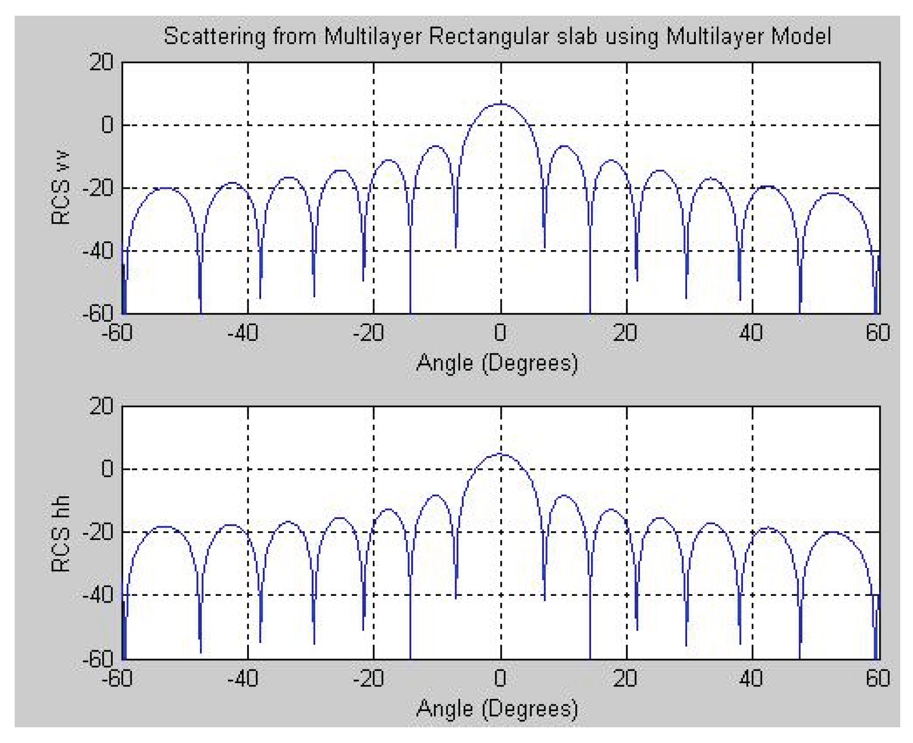
Using multilayer model the radar cross section is obtained.
Figure 12.
Example of a multi-layer model rectangular figure.
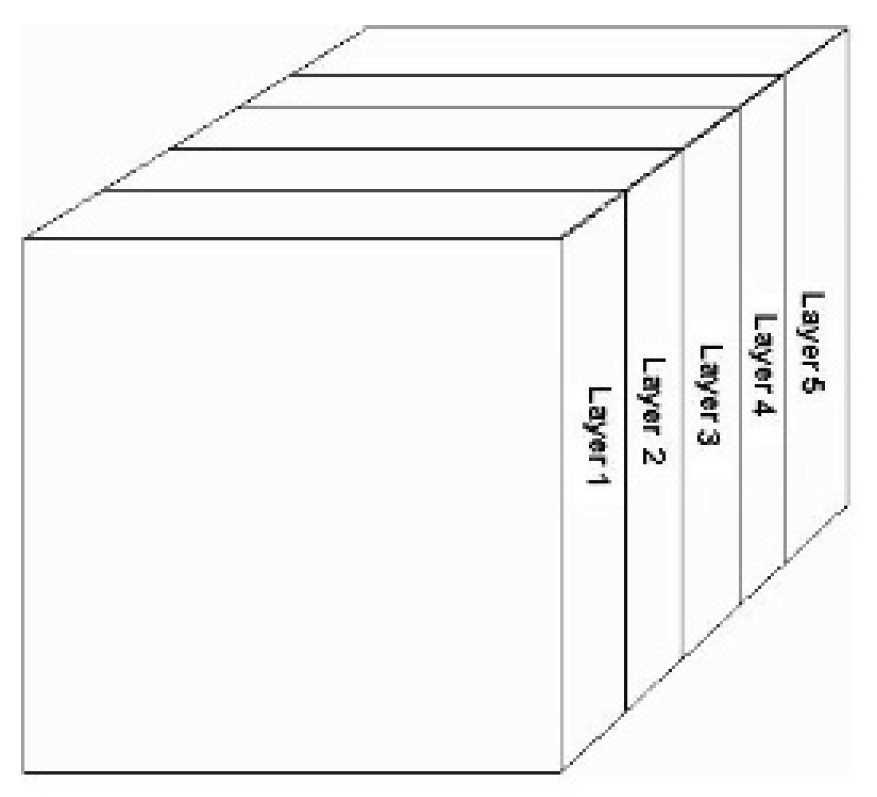

Table 1.
Properties of the rectangular& circular multi-layer figure.
| Layer number | Dielectric constant | Loss tangent | Thickness |
| 1 | 4.30 | 0.015 | 0.0030 |
| 2 | 1.15 | 0.005 | 0.0102 |
| 3 | 4.30 | 0.015 | 0.0030 |
| 4 | 3.15 | 0.035 | 0.0013 |
| 5 | 7.30 | 0.270 | 0.0002 |
Figure 13.
Radar cross section of the multi-layer example.
Let’s consider a multi-layered circular structure shown below and obtain its radar cross section using the proposed method:
Figure 14.
Example of a multi-layer circular figure.
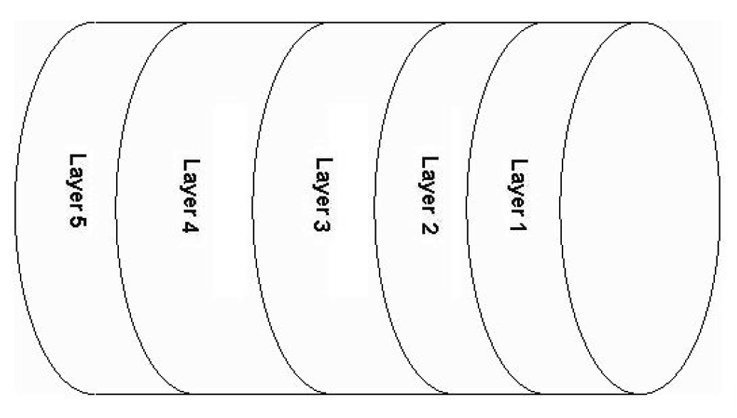
Figure 15.
Radar cross section of the circular multi-layer figure.
5. Pulse Propagation Through Wall
Bandwidth is the range between the highest and lowest frequencies within a continuous spectrum of frequencies. It is conventionally quantified in hertz. The fractional bandwidth (FBW) of an antenna quantifies its wideband characteristics. FBW is defined when it works at a center frequency fc, which lies between the lower frequency f1 and the upper frequency f2, where fc is calculated as (f1+f2)/2.
FBW varies between 0 and 2, in addition it is often quoted as a percentage (between 0% and 200%). The higher the percentage, the wider the bandwidth. Wideband antennas typically have a Fractional Bandwidth of 20% or more. Antennas with a FBW of greater than 50% are referred to as ultra-wideband antennas [16].
Ten different wall materials commonly encountered in building environments are selected for characterization [18]. These include drywall, glass, wallboard, styrofoam, cloth office partition, wooden sample door, wood, structure wood, brick, concrete block, and reinforced concrete column. The signal is reflected anytime there is a change in material inside each zone, as seen in for a single layer in Figure 1. The graphic depicts a basic model of signal reflection, demonstrating the reflection at the boundary of the region. The signal reflects upon reaching the following area, subsequently reflects again at the end of that region, and this process perpetuates until the energy of the reflected signal is deemed minimal.
An essential notion in fundamental propagation is the recognition that the total received signal comprises the summation of all reflected signals. Electromagnetic wave reflection transpires when a wave hits a discontinuity in the characteristic impedance of the propagation medium, indicating that the wave is reflected upon meeting a material distinct from its current medium. The total reflection from a complex target is contingent upon the electrical dimensions of all reflectors, their spatial arrangements, and the angle of reflection of the re-radiated signal [19]. The angle of incidence also influences the perceived reflectivity. The initial reflection’s arrival is visually evident from the received signal. This information can accurately ascertain the distance from the antenna to the wall. Determining the wall thickness, d, is complex due to the absence of a definitive visual answer from the received information. As a signal traverses a material, it is modified by the material’s characteristic impedance.
A designed basic model in MATLAB providing a clear depiction of how the signals propagate through different building materials of walls of varying widths. This model allows the ability for the user to change the building material, wall thickness, and location of the radar antennas. In this model not only the wall’s type is described with the transmitting and the receiving signals, but the majority of the requirements for a signal propagation modeling software is also defined. The model used in this study has the capability for modeling signal propagation through any type of material.
In the theoretical part, the material characteristics need to be identified in order to determine how various materials affect the propagation of the UWB radar signals. Therefore material characteristics as permeability and permittivity by µ and ε are defined respectively. Sampling frequency is chosen to be 16 GHz, and variance 0.5. Gaussian function and its frequency response are defined as the following accordingly:
y=20log(H(jw))
First derivative and the second derivative of the Gaussian function are defined as the following:
f’(x)=(t/σ2)f(x)
f’’(x)=(1/σ2-t2/σ4)f(x)
γ that is the complex propagation constant given as:
where α is the attenuation constant and β denotes the phase constant.
Transfer function H(jw) to obtain received and reflected signals is obtained as the following:
where d is the thickness of the material and
Received signal for multi-layer case is simulated in this part. Adding a new layer to system causes time shifting and causes to decrease magnitude of received signal. In Figure 16 received signal after first layer is shown. Magnitude of transmitted signal decreases and this layer causes time-shifting. Relative permittivity of the wall is 4.2 and thickness is chosen 20 cm.
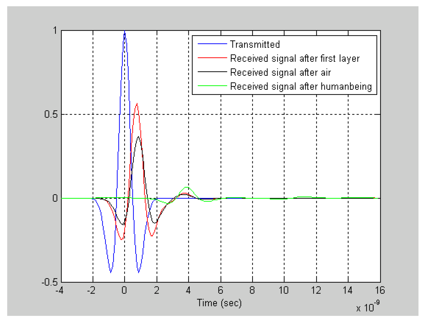
After the first layer, signal propagates through air to reach humanbeing who is wanted to detect. Loss in the air is lower than that in the wall (Figure 17). In Figure 18, signals propagating through humanbeing is depicted. Relative permittivity of humanbeing varies due to signal frequency and body parts which signal propagates. In this code, relative permittivity is chosen 45 for muscle and signal frequency is chosen 8 GHz [19,20].
This section of the research demonstrated that ultra-wideband pulses exhibit varying behaviors contingent upon the type and thickness of the barriers they traverse. The simulations showed that each new layer slowed down the signal and made it weaker. Air gaps, on the other hand, caused less loss than thick materials. The signals changed their behavior when they reached the human body behind a wall because the properties of the tissue were different. This suggests that it is possible to find people based on these effects. These results show that the model can accurately simulate how signals interact with walls and bodies. This makes it handy for things like through-wall sensing and finding people.
6. Conclusions
This study employed a multilayer modeling technique to forecast the radar cross section (RCS) of slabs with varying forms, materials, and frequencies. The simulation findings closely aligned with experimental measurements and existing reference models, thereby validating the method’s accuracy and reliability. The method demonstrated adaptability, yielding effective results for both circular and rectangular multilayer configurations. In addition to RCS estimates, the study investigated the propagation of ultra-wideband signals through typical construction materials, demonstrating its capability to ascertain wall thickness and locate humans concealed behind barriers. Collectively, these findings indicate that the model functions as both a valuable instrument for radar research and a pragmatic solution for applications including sensing, monitoring, and search-and-rescue operations.
The proposed multi-layer model for radar cross-section estimate can be utilized to determine the backscattering of multilayered objects. The simulation results align with experimental data and demonstrate advantages at certain angles compared to existing literature. Following our formulation that aligns with experimental evidence, the multilayer model can be further expanded to serve as a model for bigger systems. This concept of modeling large-scale macro systems, such as vegetation, landscapes, or clouds, can be applied in future study. These are crucial for modeling and engineering electromagnetic propagation and remote sensing.
Furthermore, the study highlights that the practical effectiveness of the proposed multilayer model in through-wall human detection is strongly influenced by factors such as the number of individuals, their movements, and surrounding environmental conditions. The actions of an individual are defined by their mobility (walking or sitting). This substantially affects their detection. A moving individual is more readily detectable than a seated or recumbent individual. In this scenario, the individual can be identified only based on their respiratory or cardiac activities. Monitoring respiratory and cardiac activity is, nevertheless, a formidable undertaking, particularly when individuals are positioned behind obstructions.
Author Contributions
Conceptualization, S. S. Seker and F. Callialp; methodology, S. S. Seker.; software S. S. Seker; validation, S. S. Seker and F. Callialp; formal analysis, S. S. Seker; investigation, S. S. Seker; resources, F. Callialp; data curation, F. Callialp; writing—original draft preparation, F. Callialp; writing—review and editing, S. S. Seker and F. Callialp; visualization, F. Callialp; supervision, S. S. Seker; project administration, F. Callialp. All authors have read and agreed to the published version of the manuscript.
Conflicts of Interest
The authors declare no conflicts of interest.
Abbreviations
The following abbreviations are used in this manuscript:
| RCS | Radar Cross Section |
| UWB | Ulta-Wideband |
| SNR | Signal to Noise Ratio |
| PRF | Pulse Repetition Frequency |
| FBW | Fractional bandwidth |
References
- Ruck, G.T.; Barrick, D.E.; Stuart, W.R.; Kirchbaum, C.K. Radar Cross Section Handbook, Vol. 2, New York: Plenum, 1970.
- Weil, H.; Chu, C.M. Integral equation method for scattering and absorption of electromagnetic radiation by thin lossy dielectric disks. J. Comput. Phys. 1976, Volume 22, No. 1, pp. 111-124.
- Le Vine, D.M.; Schneider, A.; Land, R.H.; Seker, S.S. Scattering from arbitrarily oriented dielectric disks in the physical optics regime. J. Opt. Soc. Am. 1983, Volume 73, No. 10, pp. 1255-1262.
- Bhattacharyy, A.K.; Sengupta, D.L. Radar Cross Section Analysis and Control, Artech House, ch. 1-2, 1991.
- Schipper, T.; Guasch, J.F.; Tarchi D. RCS Measurement Results for Automotive Related Objects at 23-27 GHz, Proceedings of the 5th European Conference on Antennas and Propagation (EUCAP), Rome, Italy, 11-15 April 2011.
- Skolnik, M. Role of radar in microwaves. IEEE Trans. Microw. Theory Tech. 2002, Volume 50, No. 3.
- Paris, D.T.; Hurd, F.K. Basic Electromagnetic Theory, McGraw-Hill Book Company, ch. 7-8, 1969.
- Huang, E.; Delude, C.; Romberg, J. Anisotropic Scatterer Models for Representing RCS of Complex Objects. 2021 IEEE Radar Conference, Atlanta USA, 07-14 May 2021.
- Zhang, Y.; Jiao, Y.; Zhu, M. Wideband near-field RCS measurement techniques with improved far-field RCS prediction accuracies. IEEE Trans. Instr. Meas. 2023, Volume 72, 8000404.
- Le Vine, D.M.; Schneider, A.; Lang, R.H.; Carter, H.G. Scattering from thin dielectric disks. IEEE Trans. Antennas Prop. 1984, Volume 33, no. 12, 1984.
- Dunde, V.; Tabassum, A.; Mandala, N.S.; Jangam, T.; Palnati, J. Implementation of RCS for Simple and Complex Objects. 2022 International Conference on Recent Trends in Microelectronics, Automation, Computing and Communication Systems (ICMACC), Hyderabad, India, 2022, pp.1-6.
- Ren, Z.; Chen, Q.; Jiang, T. RCS Analysis of Offshore Wind Turbines. 2024 IEEE 7th International Conference on Electronic Information and Communication Technology (ICEICT), Xi’an, China, 2024. pp. 1513-1515.
- Jarvis, R.E.; Metcalf, J.G.; Ruyle, J.E.; McDaniel, J.W. Wideband measurement techniques for extracting accurate RCS of single and distributed targets. IEEE Trans. Instrum. Meas. 2022, Volume 71, pp. 1-12.
- Bimpas, M.; Nikellis, K.; Paraskevopoulos, N.; Econonou, D.; Uzunoglu, N. Development and Testing of a Detector System for Trapped Humans in Building Ruins. 33rd European Microvawe Conference Vol.3 pp. 999-1002, October 2003.
- Arai, I. Survivor Search Radar System for Person Trapped under Earthquake Rubble. Proceeding of the IEEE Microwave Conference Vol.2 pp.663-668, December 2001.
- Fractional Bandwidth. Available Online: https://www.antenna-theory.com/definitions/fractionalBW.php (accessed on 10.08.2025).
- United States. DARPA NETEX program. Ultra-wideband channel propagation measurements and channel modeling. Through-the-Wall Propagation and Material Characterization. Blacksburg, CA: 18.11.2002.
- A. G. Yaroyov, UWB Radar for Human Being Detection. read.pudn.com/.../UWB%20radar%20for%20human%20being%20detection.pdf.
- Taylor, James D. Introduction to Ultra-wideband Radar Systems. Boca Raton, FL: CRC Press, Inc., 1995.
- Şeker, Ş.S.; Alkocoglu I.; Callialp, F. Ultra-wideband waves through multilayer planer, cylindrical and spherical models. Int. J. Eng. Tech. Manag. Res. 2020. Volume 7, No. 7,pp. 58-70, Dec. 2020.
Figure 2.
Le Vine’s simulation result of case 1 for both vertical and horizontal polarization at 4 GHz.
Figure 2.
Le Vine’s simulation result of case 1 for both vertical and horizontal polarization at 4 GHz.
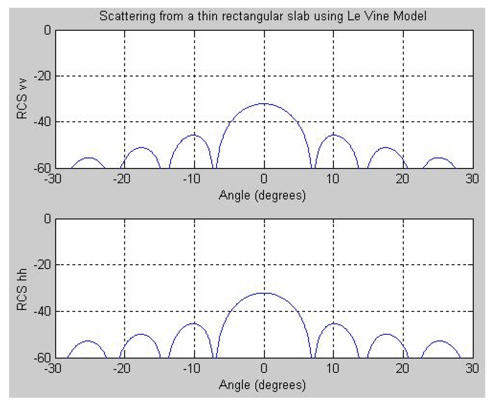
Figure 3.
Multi-layer model simulation result of case 1 for both vertical and horizontal polarization at 4 GHz.
Figure 3.
Multi-layer model simulation result of case 1 for both vertical and horizontal polarization at 4 GHz.
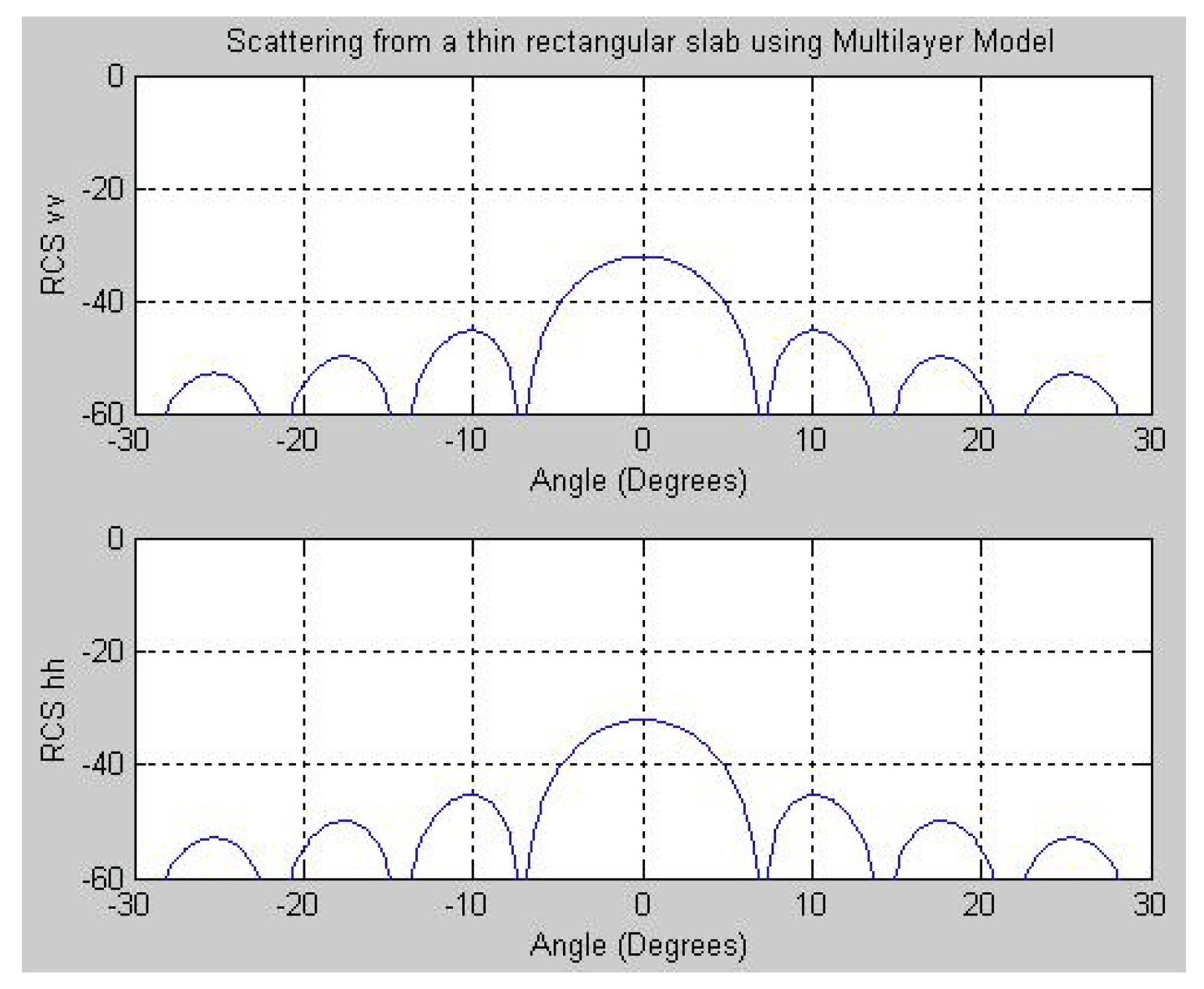
Figure 4.
Le Vine’s simulation result of case 1 for both vertical and horizontal polarization at 16 GH.
Figure 4.
Le Vine’s simulation result of case 1 for both vertical and horizontal polarization at 16 GH.
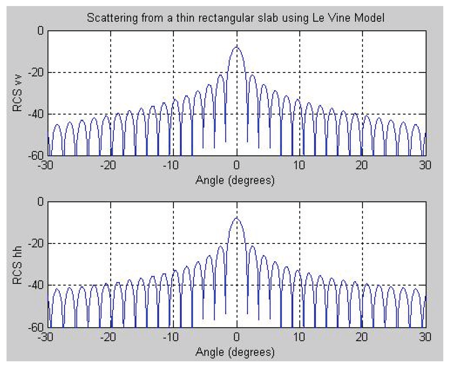
Figure 5.
Multi-layer model simulation result of case 1 for both vertical and horizontal polarization at 16 GHz.
Figure 5.
Multi-layer model simulation result of case 1 for both vertical and horizontal polarization at 16 GHz.
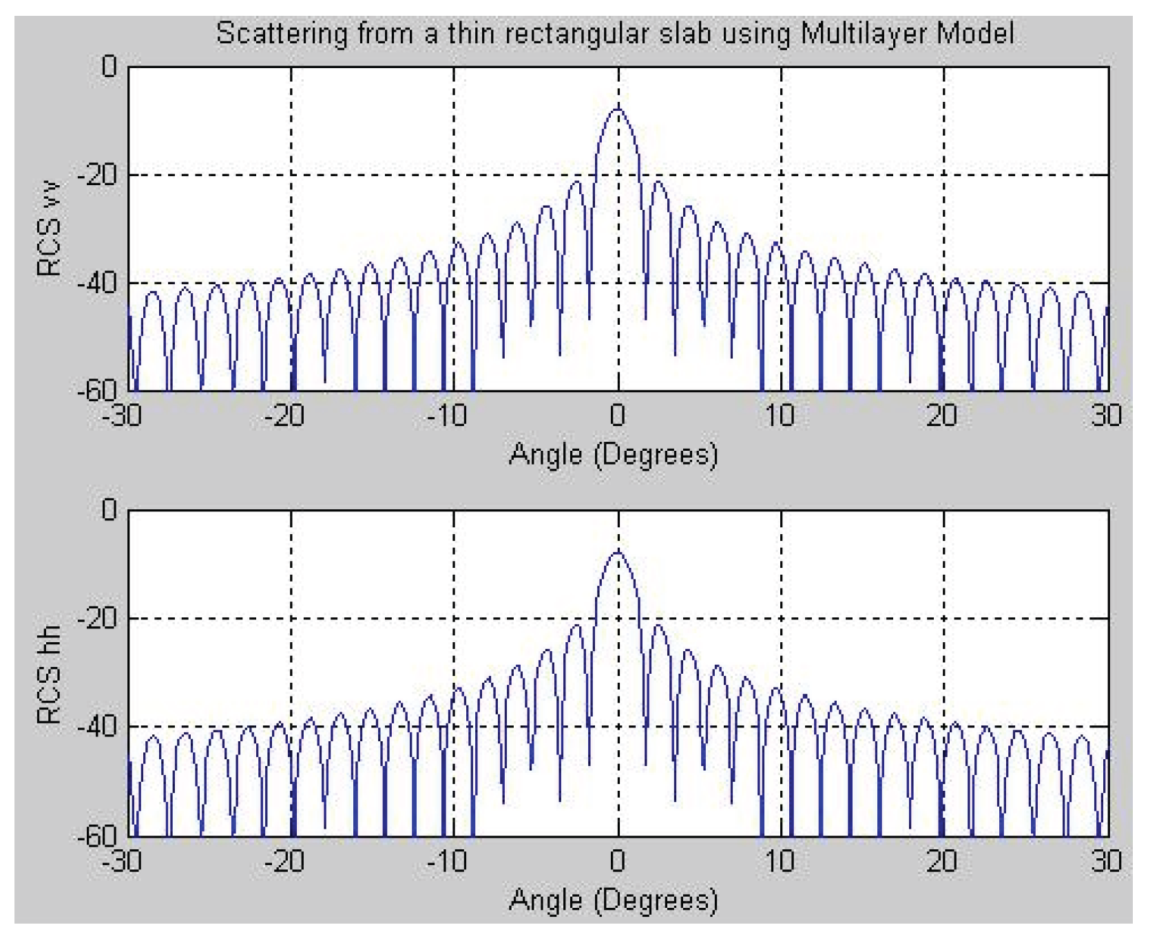
Figure 6.
Le Vine’s simulation result of case 2 for both vertical and horizontal polarization at 9 GHz.
Figure 6.
Le Vine’s simulation result of case 2 for both vertical and horizontal polarization at 9 GHz.

Figure 7.
Multi-layer model simulation result of case 2 for both vertical and horizontal polarization at 9 GHz.
Figure 7.
Multi-layer model simulation result of case 2 for both vertical and horizontal polarization at 9 GHz.
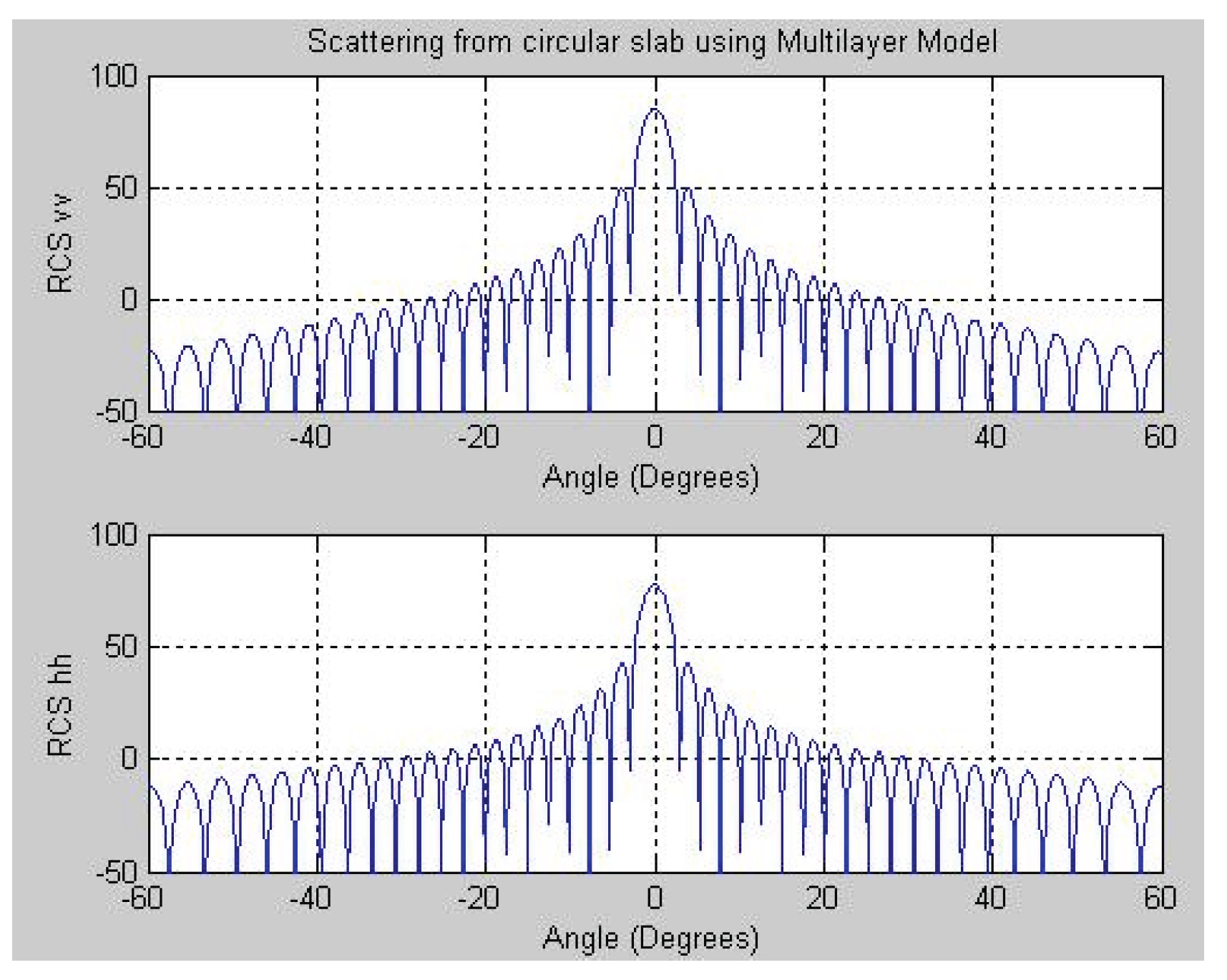
Figure 8.
Le Vine’s simulation result of case 3 for both vertical and horizontal polarization at 5 GHz.
Figure 8.
Le Vine’s simulation result of case 3 for both vertical and horizontal polarization at 5 GHz.
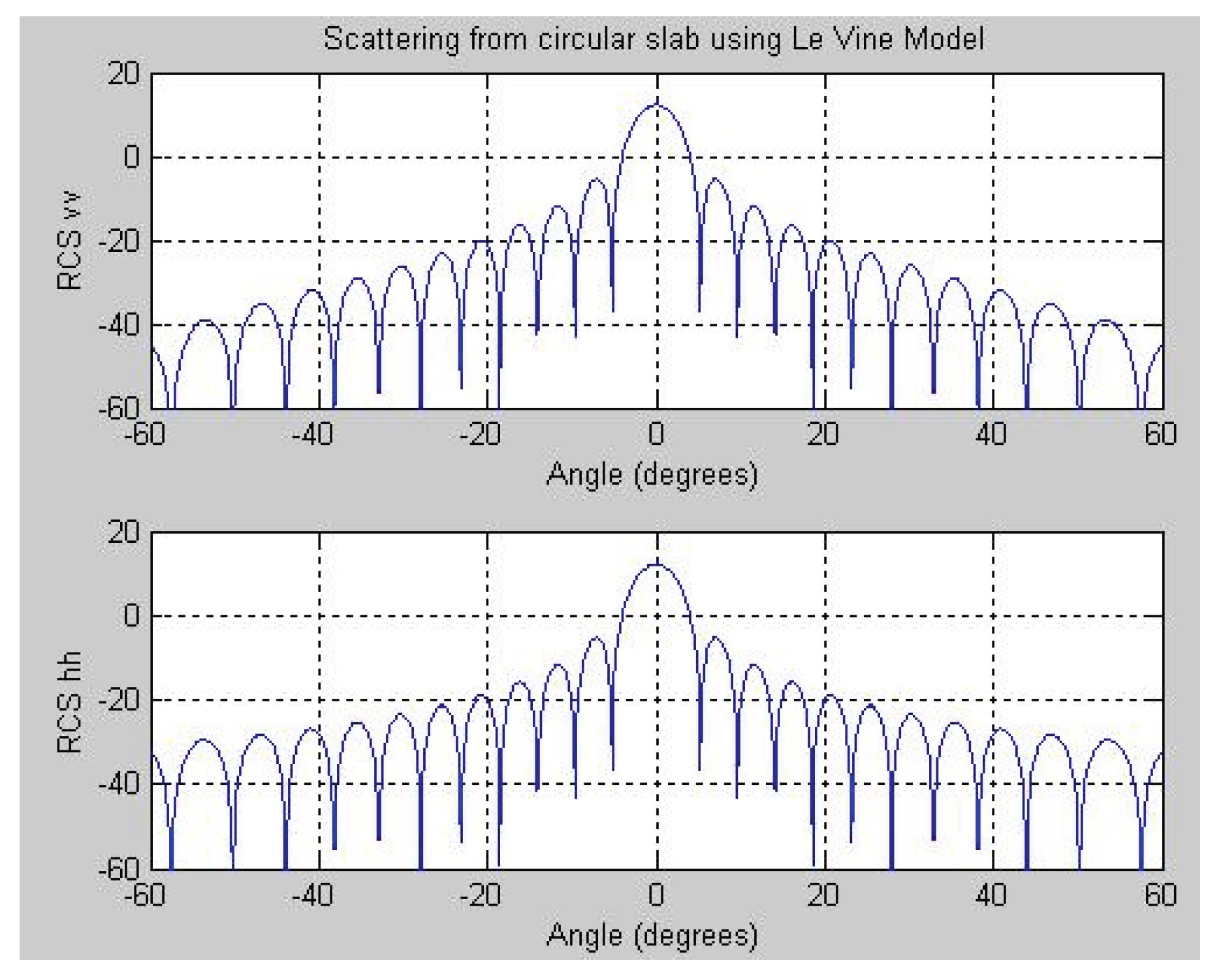
Figure 9.
Multi-layer model simulation result of case 3 for both vertical and horizontal polarization at 5 GHz.
Figure 9.
Multi-layer model simulation result of case 3 for both vertical and horizontal polarization at 5 GHz.
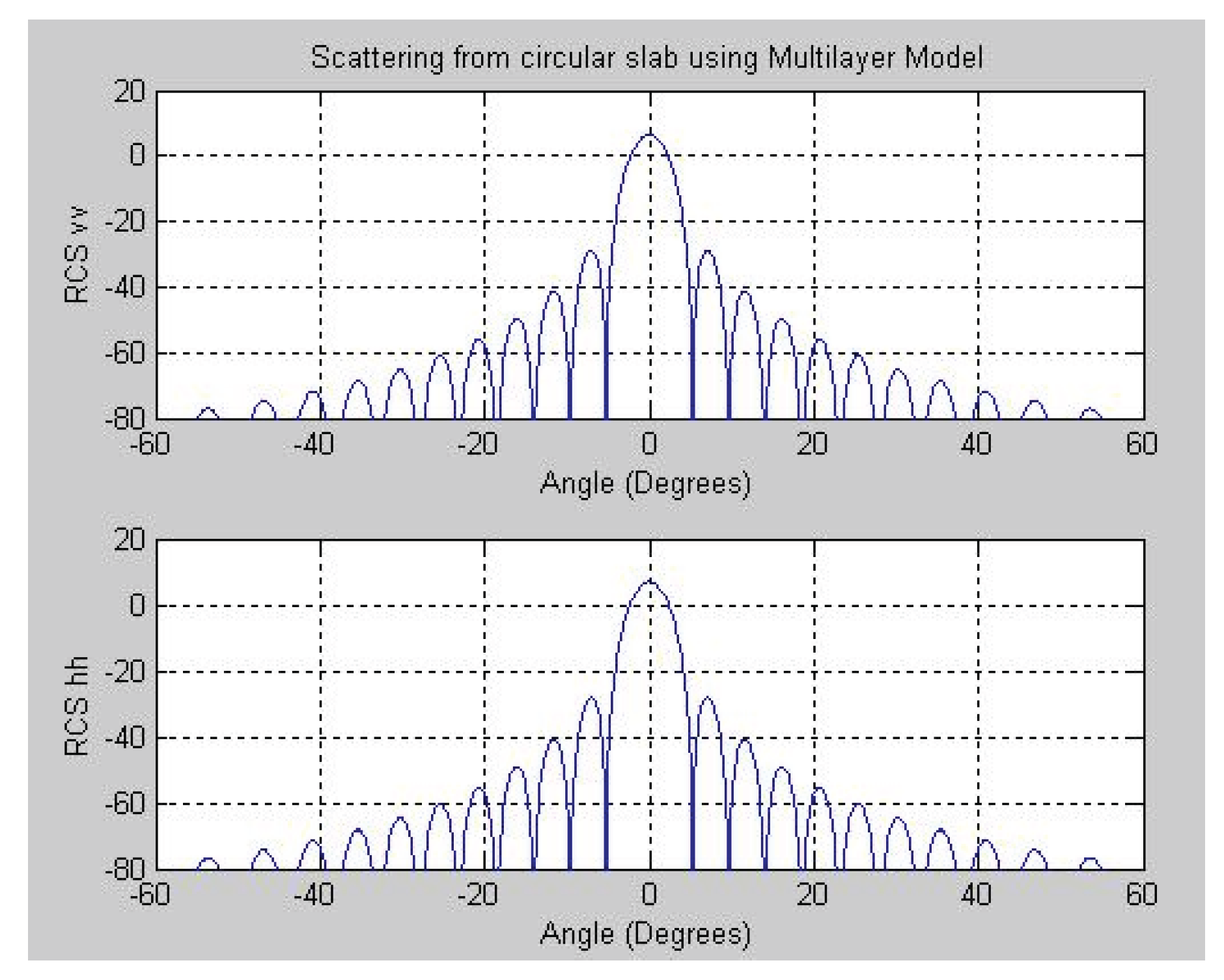
Figure 10.
Le Vine’s simulation result of case 4 for both vertical and horizontal polarization at 9 GHz.
Figure 10.
Le Vine’s simulation result of case 4 for both vertical and horizontal polarization at 9 GHz.
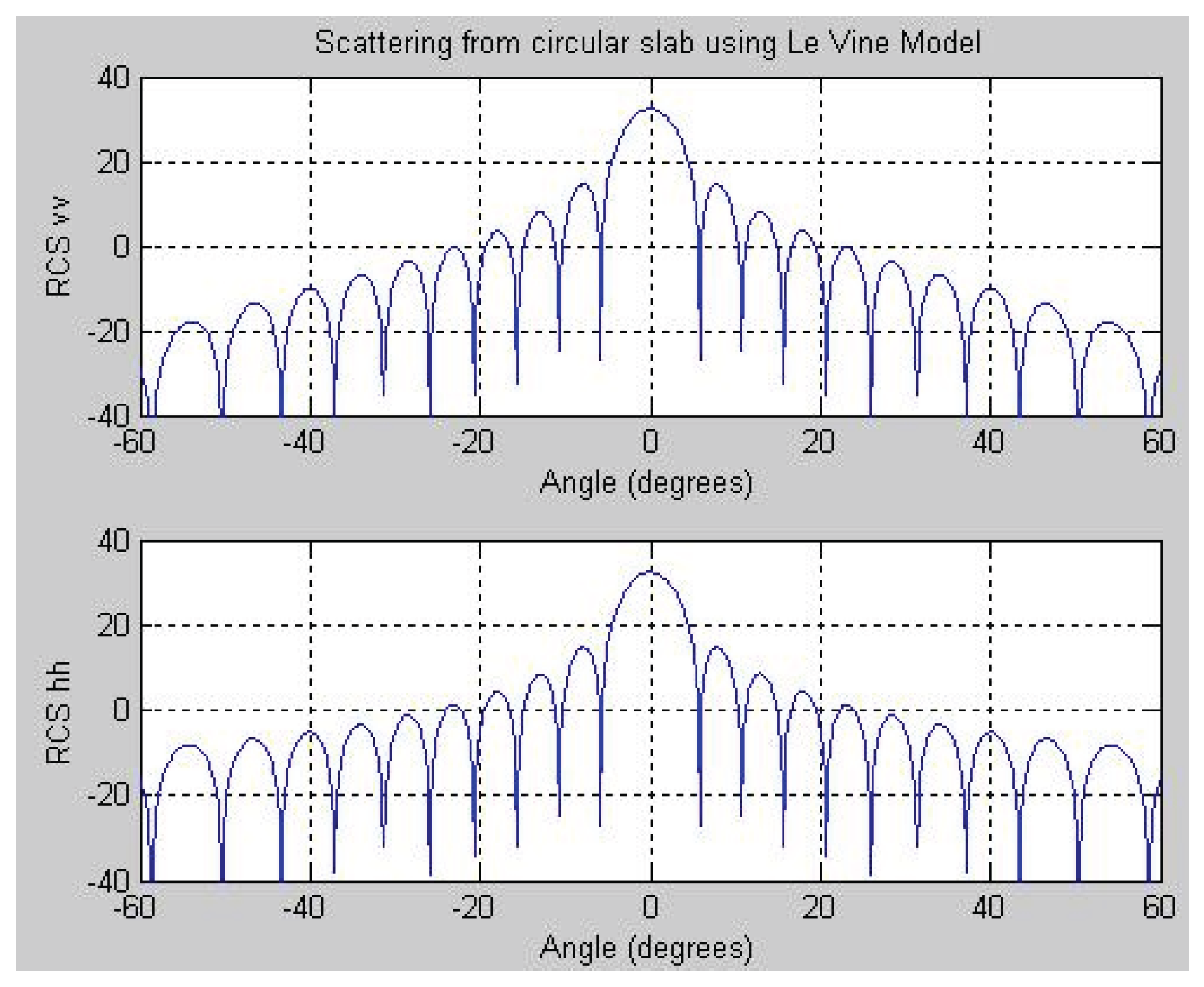
Figure 11.
Multi-layer model simulation result of case 4 for both vertical and horizontal polarization at 9 GHz.
Figure 11.
Multi-layer model simulation result of case 4 for both vertical and horizontal polarization at 9 GHz.
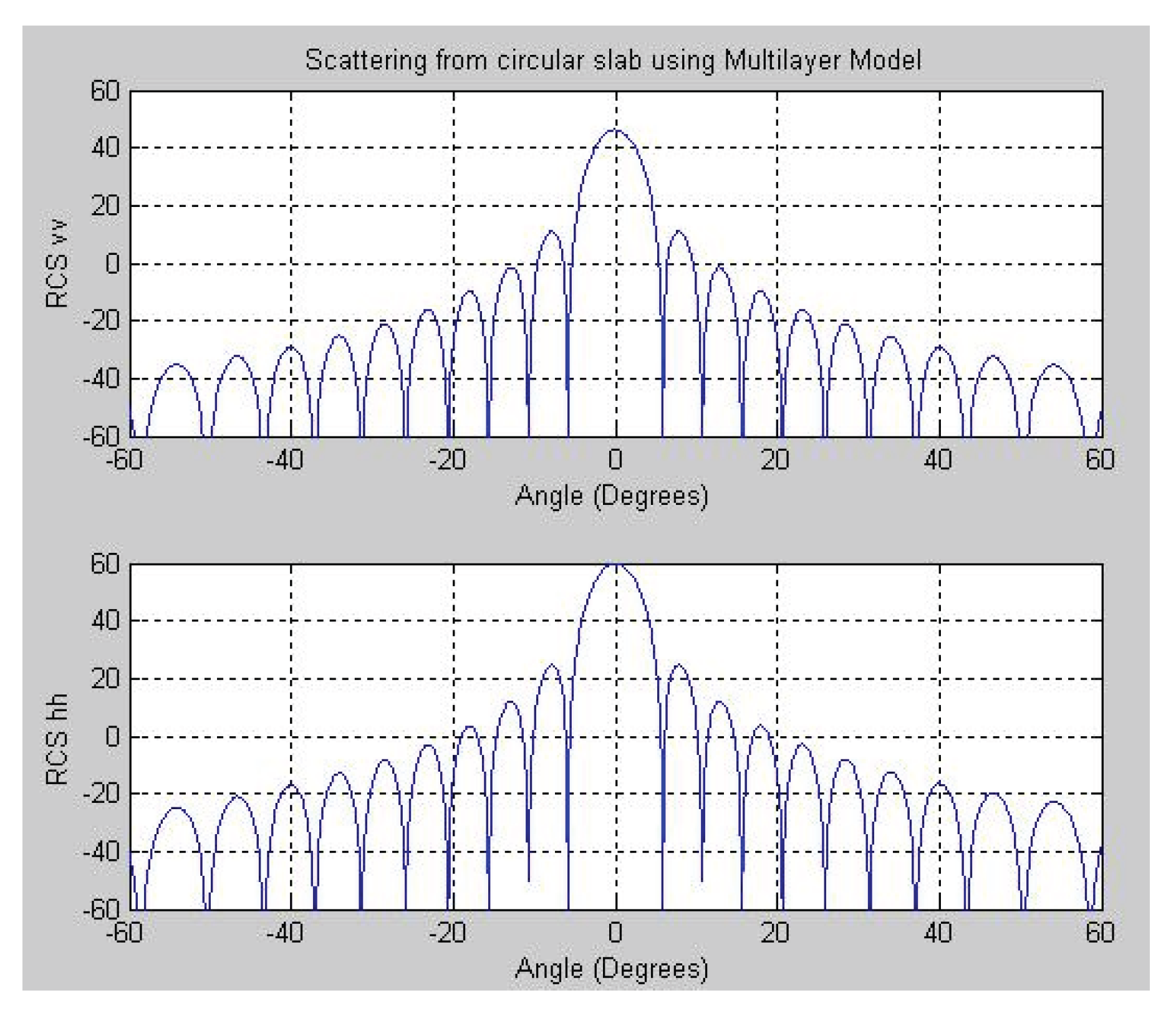
Figure 16.
Transmitted and received signal for εr=4.2 d=0.20 m, σ=0.5x10⁻⁹ and fs=8 GHz.
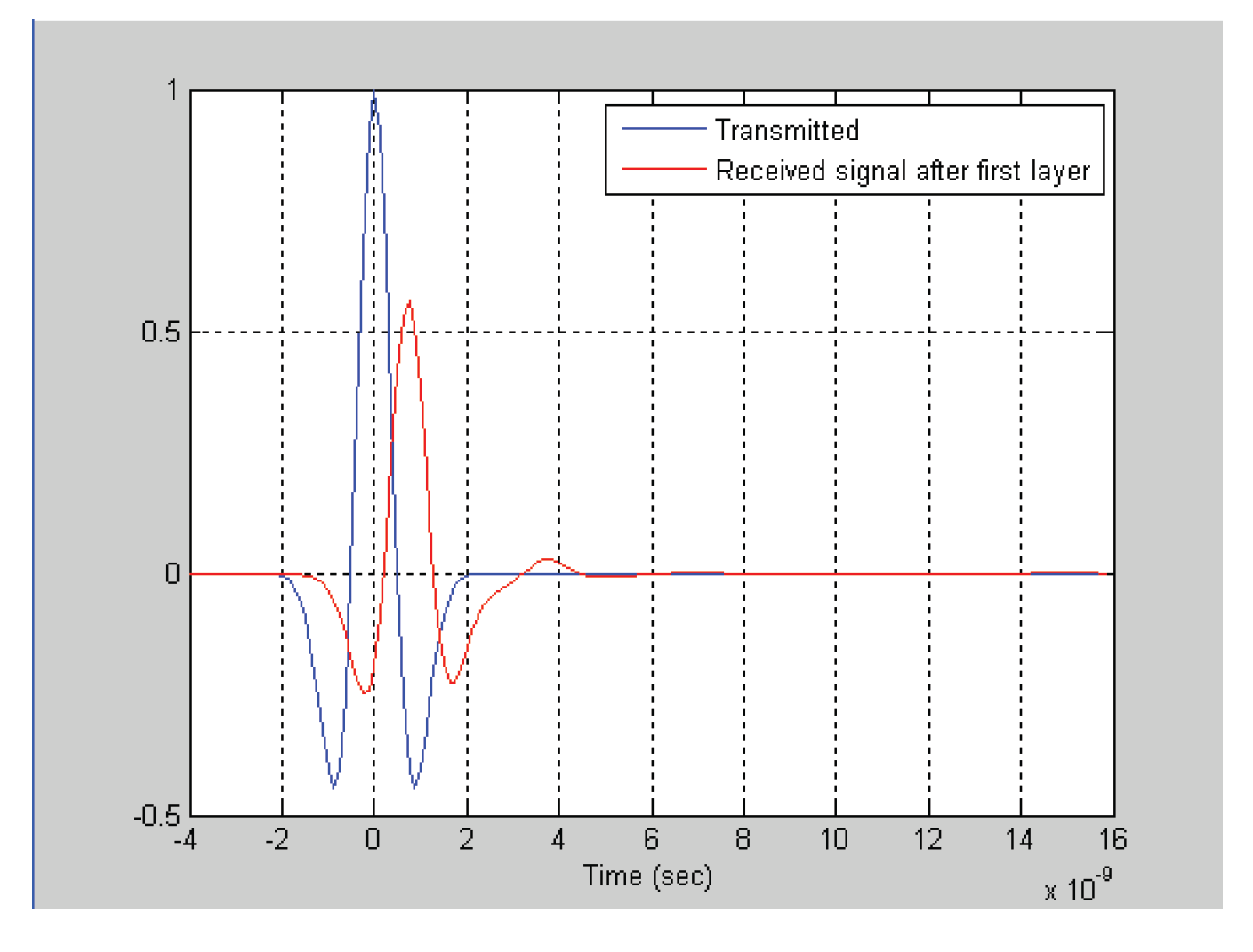
Figure 17.
Transmitted and received signal for εr=1.05 dair=0.5 m, σ=0.5x10⁻⁹ and fs=8 GHz.
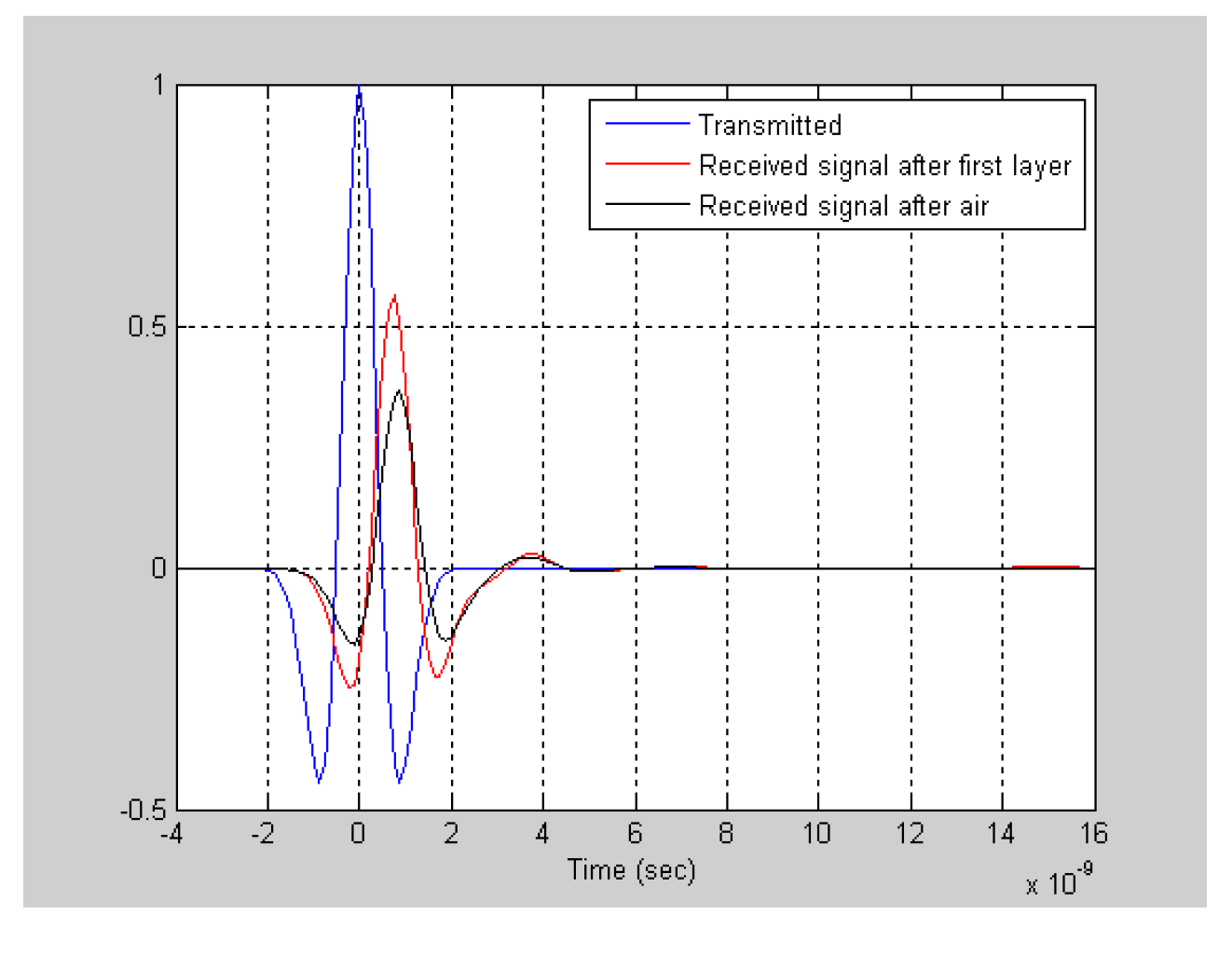
Figure 18.
Transmitted and received signal for εr=45 dbb=0.15 m, σ=0.5x10⁻⁹ and fs=8 GHz.
Disclaimer/Publisher’s Note: The statements, opinions and data contained in all publications are solely those of the individual author(s) and contributor(s) and not of MDPI and/or the editor(s). MDPI and/or the editor(s) disclaim responsibility for any injury to people or property resulting from any ideas, methods, instructions or products referred to in the content. |
© 2025 by the authors. Licensee MDPI, Basel, Switzerland. This article is an open access article distributed under the terms and conditions of the Creative Commons Attribution (CC BY) license (http://creativecommons.org/licenses/by/4.0/).
Copyright: This open access article is published under a Creative Commons CC BY 4.0 license, which permit the free download, distribution, and reuse, provided that the author and preprint are cited in any reuse.


