
Submitted:
21 August 2025
Posted:
22 August 2025
Read the latest preprint version here
Abstract
A reinforced concrete (RC) moment-resisting frame (MRF) with steel damper columns (SDCs) can be considered a damage-tolerant structure. SDCs behave as sacrificial members that absorb seismic energy prior to RC beams and columns. The behavior of such a structure depends on the strength balance of the RC MRF and SDCs, and the pinching behavior of RC members. In this article, the seismic behavior of an RC MRF with SDCs under pulse-like ground motion sequences is investigated by applying an extended incremental critical pseudo-multi-impulse analysis (ICPMIA). This article consists of two analytical studies. The first focuses on (a) the degradation in energy dissipation of an RC MRF with SDCs and (b) the increase in response period due to prior earthquake damage. An extended ICPMIA of RC MRF models is carried out. The second analytical study focuses on the influence of the pulse period of pulse-like ground motion sequences on the response of RC MRFs with SDCs. The main findings are as follows. (1) When the pulse velocities of the two multi impulses (MIs) are the same in sequential MIs, the peak displacement is larger than that of a single MI if the first and second MI have the same sign. This trend is notable when the SDC strength is relatively low, and the pinching behavior of RC beam is significant. (2) The degradation in energy dissipation of an RC MRF in the second input is notable when the pinching behavior of RC beams is significant and the SDC strength is relatively low, whereas such degradation is limited when the SDC strength is relatively high. (3) The increase in RC MRF response period in the second input is notable when the pinching behavior of RC beam is significant. (4) For nonlinear time history analysis (NTHA) using sequential ground pulses, the most critical period of the second pulse is longer than that of a single pulse. (5) The most critical response obtained from NTHA for the pulses in (4) can be approximated by the extended ICPMIA results.
Keywords:
reinforced concrete moment-resisting frame
; steel damper column
; earthquake sequence
; incremental critical pseudo-multi impulse analysis
; pulse-like ground motion
; maximum momentary input energy
1. Introduction
1.1. Background and Motivations
Strong earthquakes, which cause moderate to severe
damage to building structures, often occur as a series of earthquake sequences,
not as a single event. In past major seismic events such as the 2011 off the
Pacific coast of Tohoku Earthquake in Japan, the 2016 Kumamoto Earthquake in
Japan, and the 2023 Kaharamanmaraş Earthquake in Turkey), strong aftershocks
occurred following the mainshock, forming foreshock–mainshock sequences. In
addition, a pair of seismic events closely spaced in time and location (doublet
earthquakes) occurred in northwest Iran in August 2012 (Yaghmaei-Sabegh, 2014).
Therefore, the nonlinear response of a building structure subjected to an
earthquake sequence is important. It is very important to mention that the
interval between two severe seismic events (e.g., the mainshock and the major
aftershock) may be very short (a few hours or a few days). Therefore, the
restoration of damaged structural members cannot be completed before the next
strong seismic event. In a reinforced concrete (RC) moment-resisting frame
(MRF), stiffness and strength are degraded by the cracking of concrete,
yielding of reinforcement, and deterioration of concrete–steel bonding. Such
degradation causes an increase in the natural period and deterioration in energy
dissipation capacity of the whole structure. Therefore, the nonlinear
characteristics of a damaged RC MRF are different from those of a non-damaged
one.
The steel damper column (SDC) (Katayama et al.,
2000) is an energy-dissipating device (damper) suitable for mid- and high-rise
RC housing buildings. SDCs can be easily installed in an RC MRF because they
minimize obstacles in architectural planning. An RC MRF with SDCs can be
considered a damage-tolerant structure (Wada et al., 2000). SDCs behave as sacrificial
members that absorb seismic energy prior to RC beams and columns. Therefore,
such structures are expected to minimize unfavorable changes in structural
characteristics of buildings due to the accumulated damage during the
earthquake sequences. In a previous study (Fujii, 2025a), the author
investigated the nonlinear seismic response of an eight-story RC MRF with SDCs
subjected to the recorded ground motion sequences of the 2016 Kumamoto
earthquakes. In another study, critical pseudo-multi impulse (PMI) analyses
(Akehashi and Takewaki 2022) were extended as a substitute for sequential
seismic input. The predicted peak and cumulative response of RC MRFs with SDCs
agreed with those of nonlinear time history analysis (NTHA). However, to
understand the basic behavior of RC MRFs with SDCs subjected to a sequential
seismic input, the following questions still need to be solved:
- a)
- The strength balance of the RC MRF and SDCs is a point of interest for seismic design. How will the behavior of such a structure under earthquake sequences change as the strength balance of the RC MRF and SDCs changes?
- b)
- How is the hysteretic dissipated energy of a damaged RC MRF with SDCs different from that of a non-damaged RC MRF with SDCs? When the pinching behavior of RC beam is notable, the hysteretic dissipated energy of RC members deteriorates significantly. Because the behavior of SDC is influenced by the surrounding RC beams, the hysteretic dissipated energy of an SDC depends on the behavior of surrounding RC beams. How will the hysteretic dissipated energy of SDCs change owing to the prior damage to surrounding RC beams?
- c)
- The natural period of a damaged RC MRF is longer than that of a non-damaged RC MRF (e.g., Di Sarno and Amiric, 2019). How will the increase in the natural period of a damaged RC MRF with SDCs change as the strength balance of this structure changes? How will the pinching behavior of RC beam affect the increase in the natural period of a damaged RC MRF with SDCs?
This study focuses on the nonlinear behavior of an
RC MRF with SDCs under a pulse-like earthquake sequence.
The responses of structures under pulse-like ground
motions have been widely investigated, especially after the 1994 Northridge and
1995 Kobe earthquakes. Alavi and Krawinkler (2000; 2004) investigated the
response of generalized steel MRF models using a rectangular-pulse wave model.
They demonstrated that the response of each MRF model strongly depends on the
ratio of the pulse period () to the fundamental period () of that model: if is larger than unity, the response of the MRF
model is governed by the fundamental mode, whereas the contribution of the
higher modes to the entire response is obvious when is smaller than unity. Mavroeidis et al. (2004)
investigated the response of elastic and inelastic single-degree-of-freedom
(SDOF) systems subjected to near-fault ground motions using the velocity pulse
model proposed in their previous study (Mavroeidis and Papageorgiou, 2003).
They pointed out that using the pulse period () and amplitude () “effectively normalized the elastic and inelastic
response spectra of SDOF systems subjected to actual near-fault records.” Xu et
al. (2007) considered the response of an SDOF model with nonlinear viscous and
hysteretic dampers subjected to the velocity pulse model: they investigated the
relationship between the energy response of the model and .
These studies emphasized that the ratio of the
pulse period () to the fundamental structure period () is a key parameter for the response of a building
subject to pulse-like ground motions. As mentioned above, the fundamental
period of a damaged RC structure becomes longer owing to the damage caused by
previous seismic events. Therefore, the relation between the pulse period and
the fundamental period of a damaged RC structure is important for studying the
response of such a structure to an earthquake sequence.
Mahin (1980) studied the response of an SDOF model
with elastic–perfectly-plastic hysteresis subjected to a mainshock–aftershock
sequence. To this author’s knowledge, this was the oldest study on this issue.
Following this study, many researchers have investigated the responses of
structures under earthquake sequences by conducting NTHA. Most of these studies
can be divided into two groups according to the ground motion sequences: as-recorded
ground motion sequences and “artificial” ground motion sequences [e.g.,
applying the same ground acceleration several times (repeated approach), or
choosing different ground accelerations at random (randomized approach)].
Amadio et al. (2003) studied the nonlinear response of an SDOF system subjected
to repeated earthquakes, applying the repeated approach. Similarly,
Hatzigeorgiou and Beskos (2009) studied the inelastic displacement ratio for
SDOF systems by applying the repeated approach. To avoid bias caused by the
repeated approach, another study by Hatzigeorgiou (2010a) applied the
randomized approach to analyze the nonlinear response of an SDOF system
subjected to multiple near-fault earthquakes. Then, Hatzigeorgiou (2010b)
analyzed the nonlinear response of SDOF systems subjected to multiple near- and
far-fault earthquakes. In addition, Hatzigeorgiou and Liolios (2010) studied
the nonlinear response of a multi-degree-of-freedom (MDOF) system subjected to
as-recorded ground motion sequences, analyzing the response of planar RC
frames. Ruiz-García and Negrete-Manriquez (2011) compared the nonlinear
responses of planar steel frames subjected to as-recorded and artificial ground
motion sequences. They concluded that the artificial sequences (repeated
approach) led to overestimation of the lateral displacement demands. They also
found that the repeated approach was insufficient to model the earthquake
sequences because the frequency characteristics of the recorded aftershocks
differed from those of the corresponding recorded mainshocks. Ruiz-García
(2012) compared the nonlinear response of frame models subjected to artificial
sequential earthquakes using both repeated and random approaches, and concluded
that the random approach would be better than the repeated approach for NTHA in
the absence of recorded earthquake sequence data. Yaghmaei-Sabegh and
Ruiz-García (2016) investigated the frequency characteristics of doublet
earthquakes that occurred in northwest Iran in August 2012 and the nonlinear
response of SDOF models. They concluded that the frequency characteristics of
the second recorded mainshock in doublet earthquakes differed from those
corresponding to the first recorded mainshock; therefore, the repeated approach
was insufficient to model the doublet earthquakes. These studies emphasized the
importance of the method of modeling earthquake sequences for conducting NTHA
of structures.
Since 2012, the number of studies on the nonlinear
response of structures subjected to earthquake sequences has been increasing.
This follows the Christchurch Earthquake in New Zealand in 2010–2011 and the
2011 off the Pacific coast of Tohoku Earthquake in Japan (e.g., Abdelnaby, and
Elnashai, 2014; Abdelnaby 2016; Di Sarno 2013; Di Sarno and Amiri, 2019).
However, the number of studies focusing on the nonlinear response of structures
subjected to near-fault earthquake sequences is still limited. Although there
are analytical studies using near-fault records as a source of artificial
seismic sequences (e.g., Hatzigeorgiou 2010a; Hatzigeorgiou 2010b; Ruiz-García
and Negrete-Manriquez 2011; Ruiz-García 2013; Yang et al. 2019), few studies
have focused on the relations between the pulse periods of the earthquake
sequences and the fundamental periods of structures.
The term “energy” is useful for understanding the
nonlinear behavior of structures (e.g., Akiyama, 1985; Akiyama, 1999; Uang and
Bertero, 1990). Recent advances in energy-based seismic engineering can be
found in the literature (Benavent-Climent and Mollaioli, 2021; Varum et al.
2023; Dindar et al. 2025). The total input energy, or the equivalent velocity of
the total input energy (), is an important seismic intensity parameter
related to the cumulative response (Akiyama, 1985; Akiyama, 1999). In addition,
the maximum momentary input energy, or the equivalent velocity of the maximum
momentary input energy (), is an important seismic intensity parameter
related to peak response (Hori and Inoue, 2002). Because the damage accumulated
in the structure is critical in earthquake sequences, it is reasonable to discuss
the response under earthquake sequences in terms of energy. Zhai et al. (2016)
analyzed the inelastic input energy spectra for mainshock–aftershock sequences.
In addition, Alıcı and Sucuoğlu (2024) analyzed the inelastic input energy
spectra of the recorded mainshock–aftershock sequences of the 2023 Kaharamanmaraş
Earthquake. Donaire-Ávila et al. (2024) and Galé-Lamuela et al. (2025) analyzed
the cumulative dissipated energy of RC building models under earthquake
sequences and then examined the applicability of Akiyama’s cumulative energy
distribution theory (Akiyama, 1985; Akiyama, 1999). They noted that “the
distribution of the cumulative dissipated energy among the stories remained
basically the same across all events within a sequence, regardless of the
design approach or the proneness of the frame to damage concentration.”
Takewaki and his group have developed an innovative
energy approach. First, Kojima and Takewaki (2015a; 2015b; 2015c) introduced
the concepts of the critical double impulse (DI) and critical multi impulse
(MI) as substitutes for near-fault and long-duration earthquake ground motion,
respectively. These concepts simplify seismic input by considering the most
severe (critical) case for the structure of interest. Then, Akehashi and Takewaki
(2021) introduced the pseudo-double impulse (PDI) and pseudo-multi impulse
(PMI) (Akehashi and Takewaki, 2022a) to form the MDOF model. In PDI and PMI
analysis, the MDOF model oscillates predominantly in a single mode, considering
the impulsive force corresponding to a certain mode vector. In addition,
Akehashi and Takewaki (2022b) proposed an adjustment to the DI method to work
like a real earthquake. The development of this theory and recent achievements
are summarized in the literature (Takewaki and Kojima, 2021; Takewaki, 2025a;
Takewaki, 2025b). Following their studies, this author has applied their PDI
and PMI analyses to an RC MRF with SDCs (Fujii, 2024a; 2024b) to verify a
simplified procedure for predicting the peak and cumulative response of an RC
MRF with SDCs based on energy (Fujii and Shioda, 2023). Then, the author
proposed an extended version of incremental critical PMI analysis (extended
ICPMIA) for predicting the nonlinear response of structures subjected to
earthquake sequences (Fujii, 2025a).
In the author’s view, the strong points of this
extended ICPMIA are (i) it can be performed if the structural model is stable
for NTHA; (ii) it automatically calculates the cumulative response of members,
which is important for discussing the accumulated damages of the structure
under earthquake sequences; (iii) the responses obtained from it can be easily
associated with ground motion using an energy spectrum as demonstrated in a
previous study (Fujii, 2025a); and (iv) its results make nonlinear structural
characteristics much easier to understand because the seismic input is
simplified. Most past analytical studies on the nonlinear response of
structures subjected to earthquake sequences have relied on NTHA using ground
motions. However, NTHA results are too complicated to derive general
conclusions, although NTHA is the most rigorous method. This is because NTHA
results are intricately intertwined with nonlinear structural characteristics
and selected ground motion characteristics. In an earthquake sequence, the
complexity increases because of the combined ground motions. As mentioned
above, the repeated approach is unrealistic for modeling the earthquake
sequence. When as-recorded ground motion sequences are used as the seismic
input of NTHA, the frequency characteristics and duration of each ground motion
in the earthquake sequence are different. Therefore, the earthquake sequence
becomes more complex.
In the extended ICPMIA, the simplification of
seismic input introduced in the original PMI is still valid: when the most
critical case is considered for the structure of interest, the timing of the
impulsive lateral force is automatically determined. The nonlinear
characteristics of the structure obtained from the extended ICPMIA are
independent of the complex frequency characteristics of selected input ground
motion sequences. This is because the frequency characteristics of input ground
motion are automatically determined from the nonlinear characteristics of the
structure itself. This is why the extended ICMPIA would be a powerful tool for
understanding the basic behavior of RC MRFs with SDCs subjected to a sequential
seismic input.
1.2. Objectives
In this article, the seismic behavior of an RC MRF
with SDCs under pulse-like ground motion sequences is investigated by applying
an extended ICPMIA. This article consists of two analytical studies. The first
focuses on (a) the degradation in energy dissipation of an RC MRF and SDCs, and
(b) the increase in response period due to prior earthquake damage. An extended
ICPMIA of RC MRF models is carried out. The first analytical study addresses
the following three questions:
- Considering the case when the pulse velocity of each MI is the same, how will the peak displacement of an RC MRF with SDCs subjected to two MIs differ from that for a single MI? How will the peak displacement of an RC MRF with SDCs subjected to two MIs be influenced by the pinching behavior of RC beams and the strength balance of the RC MRF and SDCs?
- How will the hysteretic dissipated energy of RC members of a damaged RC MRF with SDCs differ from that of a non-damaged structure, and how will the hysteretic dissipated energy of SDCs of a damaged RC MRF differ from that of a non-damaged structure?
- How will the increase in the response period of an RC MRF with SDCs be influenced by the pinching of RC beams and the strength balance of the RC MRF and SDCs?
The second analytical study focuses on the
influence of the pulse period of pulse-like ground motion sequences on the
response of RC MRFs with SDCs. An NTHA of RC MRF models with SDCs is carried
out using a model of sequential pulse-like ground motion. In this analysis, the
pulse periods of the first and second inputs are different, whereas the peak
velocities of the first and second inputs are the same. The second analytical
study addresses the following two questions:
- 1.
- Which combination of the two pulse periods produces the severest response in a given RC MRF model?
- 4.
- Considering the envelope of NTHA results and all combinations of pulse periods while the peak velocities of the first and second pulses are kept constant, can the results of the extended ICPMIA approximate the NTHA envelope?
The remainder of this article is organized as
follows. Section 2 outlines the extended
ICPMIA. Section 3 presents an RC MRF
building model with SDCs. Section 4 shows
the ICPMIA results for this building model and then discusses (i) the
relationship between the equivalent velocity of the maximum momentary input
energy of the first modal response () and the maximum equivalent displacement of the first modal response (), (ii) the response period of the first mode (), and (iii) the hysteretic dissipated energies of RC MRFs and SDCs ( and , respectively) during the first and second MIs. Then, NTHAs of RC MRFs with SDCs are carried out using models of pulse-like ground motion, and those results are compared with those of the extended critical PMI analysis in Section 5. Conclusions and further directions of this work are discussed in Section 6.
2. Outline of the Extended ICPMIA
In the following section, the extended ICPMIA is described on the basis of a previous study (Fujii, 2025a).
2.1. Extended Critical PMI Analysis
Figure 1 outlines the extended ICPMIA considering sequential input, which is presented in a previous study (Fujii, 2025a). As shown in Figure 1a,b, a planar frame building model (with stories) is subjected to a pseudo-impulsive lateral force proportional to the first mode vector (). In such cases, the frame building model oscillates predominantly in the first mode, and the contribution of the higher-modal response is negligible.
In this extended analysis, the seismic input is modeled as two component MIs. The time history of sequential ground acceleration (, : time) is modeled as a series of impulses in Equation (1):
In Equation (1), is the number of the pseudo-impulsive lateral force in the -th MI ( = 1, 2), is the ground motion velocity increment of the -th pulse in the -th MI, is the time when the -th pseudo-impulsive lateral force acts through the -th MI, is the interval length between the first and second MI, and is the Dirac delta function that satisfies Equation (2):
Here, the time of the first pseudo-impulsive lateral force in the first MI () is set to zero. In this study, is larger than or equal to 3. Therefore, is defined in Equation (3) as:
Here, is the pulse velocity in the -th MI. Note that the time between the first and second MI is defined as the length of a half cycle of the structural response.
Next, the first modal response of the building is formulated. Here, is the mass matrix of the building; , , and are the relative displacement, relative velocity, and relative acceleration vectors, respectively; and and are the restoring and damping force vectors, respectively. The equivalent displacement (), equivalent velocity (), and equivalent acceleration () of the first modal response are defined in Equations (4) to (6), respectively:
The effective first modal mass is defined in Equation (7) as
Note that and depend on the local maximum equivalent displacement within the range . In this analysis, the first mode vector at time is updated via Equation (8):
where is the time when the local maximum equivalent displacement within the range occurs. Note that, for the beginning time of the first MI ( = 0), is determined from eigenvalue analysis using the initial (elastic) stiffness, while at the beginning of the second MI() depends on the response experienced during the first MI.
The time of the action of the -th pseudo-impulsive lateral force during the -th MI is determined from the condition expressed as Equation (9):
where is the relative equivalent acceleration at time defined in Equation (10) as
The equivalent velocity of the first modal response just after the -th pseudo-impulsive lateral force during the -th MI () is calculated via Equation (11):
Here, is the equivalent velocity of the first modal response just before the action of the -th pseudo-impulsive lateral force during the -th MI. In this PMI analysis, the pseudo-impulsive lateral force is proportional to the first mode vector (), as shown in Figure 1b. Assuming that the velocity vector just before the action of the -th pseudo-impulsive lateral force during the -th MI () can be approximated as the first modal response, the corresponding velocity vector () can be approximated by Equation (12):
To calculate the response following the action of the -th pseudo-impulsive lateral force during the -th MI, the equivalent velocity just after the action of this force during the -th MI () and the corresponding velocity vector () are updated according to Equation (13):
The peak equivalent displacement during the-th MI () is obtained via Equation (14):
In Equation (14), is the time at the -th local peak of during the-th MI, as shown in Figure 1c. The peak equivalent displacement of the first modal response over the course of the entire sequential input () is obtained via Equation (15):
The energy balance of the first modal response at time can be expressed as Equation (16):
where , , , and are the kinetic energy, damping dissipated energy, cumulative strain energy, and cumulative input energy of the first modal response, defined in Equations (17) to (20) as
As shown in Figure 1, the changes in and are discontinuous at time = . The increments in and are equal to the momentary input energy of the first modal response at time . The momentary input energy of the first modal response per unit mass at time = during the -th MI () can be expressed as Equation (21):
Note that, as discussed in previous studies (Fujii, 2024a; 2025a), the momentary input energy in Equation (21) is consistent with that originally proposed by Hori and Inoue (2002). The maximum momentary input energy of the first modal response per unit mass during the -th MI () can be obtained via Equation (22):
The equivalent velocity of the maximum momentary input energy of the first modal response during the -th MI () is defined in Equation (23):
Therefore, the equivalent velocity of the maximum momentary input energy over the course of the entire sequential input () is obtained via Equation (24):
Next, the response period of the first mode during the-th MI () is defined as follows. When occurs at time = , the response period is calculated as twice the interval between the two local peaks in Equation (25):
For the case in Figure 1c, the red curve shown in the time history of the equivalent displacement () indicates the half cycle of the structural response when occurs. Therefore, because = = 3 in this case, the response period of the first mode during the first and second MIs ( and , respectively) is calculated as
The cumulative input energy of the first modal response per unit mass during the-th MI () can be obtained via Equation (26):
The equivalent velocity of the cumulative input energy of the first modal response during the -th MI () is defined in Equation (27):
Therefore, the equivalent velocity of the cumulative input energy over the entire sequential input () is obtained via Equation (28):
Next, the cumulative energies of RC members and SDCs at time ( and , respectively) are defined as follows. The cumulative strain energy of the whole structure at time is defined in Equation (29):
Then and are calculated via Equations (30) and (31), respectively:
In Equation (31), is the cumulative strain energy of the damper panel of each SDC in the -th story; and , , and are the shear force, shear strain, and height of the damper panel of each SDC in the -th story, respectively.
The cumulative strain energies of RC members and SDCs during the -th MI ( and , respectively) are calculated via Equation (32):
where and are the cumulative strain energies of RC members and SDCs just before the second MI starts, and is the ending time of the analysis.
2.2. Procedure for the Extended ICPMIA
In this study, an extended ICPMIA was carried out as follows.
STEP 1: ICPMIA considering a single MI
An ICPMIA of an -story frame building model was carried out. In this step, only a single MI was considered; the numbers of pseudo-impulsive lateral forces were set as = and = 0. The pulse velocity (= ) increased until reached the predetermined value. Then, the pulse velocity of the first MI in the extended ICPMIA () was determined as the value at which equaled the target value.
STEP 2: Extended ICPMIA considering two MIs
An extended ICPMIA of an -story frame building model was carried out. In this step, two MIs were considered; the numbers of pseudo-impulsive lateral forces were set as = = . The pulse velocity of the first MI obtained in the previous step () was used, while the pulse velocity of the second MI () increased until reached the predetermined value.
3. Building Model
The building models analyzed in this study were three eight-story housing buildings shown in Figure 2. The structural plans of the three models (Dp033, Dp050, and Dp100) are shown in Figure 2a to 2c. Model Dp100 in Figure 2c was the same model used in a previous study (Fujii, 2025a), while models Dp033 and Dp050 in Figure 2a and 2b had one-third and one-half the number of SDCs as Dp100, respectively. Frames A and B of all three models were assumed to extend infinitely in both longitudinal directions, and the colored area in Figure 2a–c was modeled for the analysis. The unit weight per floor was assumed to be 13 kN /m2. SDCs were installed only in Frame A. All RC frames were designed according to the strong-column weak-beam concept, except at the foundation beam (Lv. 0) and in the case where an SDC was installed in an RC frame. In the latter case, at the connection joint of an RC beam with an installed SDC, the RC beam was designed to be sufficiently stronger than the SDC, accounting for the strength hardening of damper panel. Sufficient shear reinforcement of all RC members was provided to prevent premature shear failure. In addition, sufficient reinforcement was provided at RC beam-RC column joint and RC beam-SDC joint to prevent joint failure. To check the strength balance of the RC MRF and SDCs, the ratio of the initial yield strength of the SDCs in the -th story () to the yield strength of the RC MRF in the -th story (), , was calculated for each model. The ranges of the ratio of models Dp033, Dp050, and Dp100 were 0.079 to 0.109, 0.119 to 0.164, and 0.238 to 0.327, respectively.
In the structural modeling, only planar behavior in the longitudinal direction was considered. All frames were connected through a rigid slab. Figure 2d shows the structure of Frame A in model Dp050. Only a two-span area was extracted from the endless longitudinal frames in DP050; therefore, the end of each boundary RC beam was supported by a horizontal roller. Figure 2e shows the structural model of Frame A in Dp100. This used the same modeling scheme as in a previous study (Fujii, 2025a). That is, only a one-span area was extracted from the endless longitudinal frames; therefore, the axial stiffness of the boundary RC columns was set to be 100 times that of the original by adjusting the sectional area. In addition, the stiffness and strength of the boundary RC columns were assumed to be one half of the original calculated value. Similar modeling schemes were applied to model Dp033. Each RC member was treated as a one-component model with a nonlinear flexural spring at each end, while each steel column was modeled as an elastic column with a nonlinear shear spring in the middle. The shear behavior of all RC members was assumed to be linearly elastic. The axial behavior of all vertical members was also assumed to be linearly elastic, so the nonlinear interaction of the axial force and bending moment of each RC column was not considered. The beam-column joint was assumed to be rigid. The natural periods of the first modal responses in the elastic ranges of models Dp033, Dp050, and Dp100 were 0.542 s, 0.520 s, and 0.459 s, respectively.
Figure 3 shows the hysteresis rule of the RC members and SDCs. This study used the same hysteresis models as in a previous study (Fujii 2025a). Here, the two models in Figure 4a,b were considered for evaluating the influence of the pinching behavior of RC beam on the response of an RC MRF with SDCs under earthquake sequences: the parameter was set to 0.25 (significant pinching) and 1.00 (no pinching). These hysteresis models are based on the Muto model (Muto et al., 1974) with two modifications. The first modification is the degradation in unloading stiffness after yielding: the unloading stiffness is modified to be inversely proportional to the square root of the ratio , where and are the peak deformation angle and yield deformation angle of RC members, respectively, as in the model of Otani (1981). The second modification is the consideration of pinching behavior. As described in a previous study (Fujii 2024b), the pinching model is assumed to be a linear combination of a perfectly non-pinching model (the Muto model with modified unloading stiffness degradation) and a perfectly pinching model. The perfectly pinching model has no hysteretic energy dissipation in symmetric loading. Therefore, for = 0.25, the hysteretic dissipated energy in symmetric loading is only 25% of that for = 1.00. No pinching was considered in RC columns for simplicity. Cyclic degradation in stiffness and strength of RC members was not considered in this analysis. For the SDC damper panel, the hysteretic (trilinear) model proposed by Ono and Kaneko (2001) and shown in Figure 4c was used. The damping matrix was assumed to be proportional to the instantaneous (tangent) stiffness without an SDC. The damping ratio of the first modal response in the elastic range of the model without an SDC was assumed to be 0.03. Second-order effects were neglected in this analysis.
4. ICPMIA of the Building Model
The analytical study in this section focused on (a) the degradation in energy dissipation of an RC MRF with SDCs and (b) the increase in the response period due to prior earthquake damage.
4.1. Analysis Method
First, an ICPMIA considering a single MI was carried out: the numbers of pseudo-impulsive lateral forces were set as = 4 and = 0. The pulse velocity was set initially at 0.1 m/s with increments of 0.05 m/s until the peak equivalent displacement of the first modal response () reached 150% of the target displacement (). Then, the value of that corresponded to was found by linear interpolation. In this analysis, was set to be 1/75 of the equivalent height (= 0.232 m), because this is the design limit assumed in the seismic design of model Dp100 in a previous study (Fujii, 2025a). Note that when reached 0.232 m, some of the RC beams and the bottom of the columns in the first story yielded, following the yielding of SDC damper panels. Therefore, the damage level of the whole model could be considered “moderate” when reached 0.232 m.
Next, an extended ICPMIA considering sequential MIs was carried out: the numbers of pseudo-impulsive lateral forces were set as = = 4. The pulse velocity of the first MI () was set as the value corresponding to , while the pulse velocity of the second MI () was set initially at 0.1 m/s with increments of 0.05 m/s until reached 150% of . As in a previous study (Fujii, 2025a), the length of intervals between the first and second MI () were set to 64 and 65. The case = 64, when the first and second MIs had opposite signs, is referred to as “Sequential-1”, while the case = 65, when the first and second MIs had the same sign, is referred to as “Sequential-2”. The ending time () was determined as the ending time of the 64th half cycle of free vibration after the action of the -th pseudo-impulsive lateral force.
A previous study by the author (Fujii, 2025b) investigated the suitable number of pseudo-impulsive lateral forces () for near-fault earthquake ground motion using the velocity pulse model by Mavroeidis and Papageorgiou (2003). It concluded that the most suitable for the velocity pulse model analyzed was 4. Therefore, was set to 4 in this study.
4.2. Analysis Results
4.2.1. Single MI
Figure 4 shows comparisons of the – relationship and the – relationship for a single MI. The results for = 0.25 (significant pinching) are shown in Figure 4a, while Figure 4b shows the results for = 1.00 (no pinching). From Figure 4(a1), the value of corresponding to = (= 0.232 m) can be found. Then, the value of corresponding to can be obtained from Figure 4(a2). The following observations can be made from Figure 4:
- For = 0.25 (significant pinching), the velocities in Dp033 corresponding to were = 1.047 m/s and = 0.5877 m/s. Similarly, those in Dp050 were = 1.108 m/s and = 0.6316 m/s, while those in Dp100 were = 1.309 m/s and = 0.7862 m/s.
- For = 1.00 (no pinching), the velocities and in all three models corresponding to were slightly higher than for = 0.25. That is, those velocities in model Dp033 were = 1.049 m/s and = 0.5888 m/s. Similarly, those velocities in Dp050 corresponding to were = 1.112 m/s and = 0.6336 m/s, while those in Dp100 were = 1.323 m/s and = 0.7967 m/s.
In the following analysis, the pulse velocity of the first MI () was set to the value in Figure 4.
4.2.2. Sequential MIs (2Vp = 1Vp)
Next, the extended ICPMIA results for = are presented. Figure 5 shows comparisons of the local response in each model in terms of the peak story drift () and the normalized cumulative strain energy of the SDC damper panel (), given by Equation (33):
In Equation (33), is the initial yield shear strain of each damper panel of the SDCs in the -th story. The following observations can be made from Figure 5:
- In models Dp033 and Dp050 ( = 0.25), for Sequential-1 was larger than that for a single MI, while in the other models, for Sequential-1 was almost the same as for the single MI. However, for Sequential-2 was larger than that for a single MI in all models.
- The values of Sequential-1 and 2 were larger than those of the single MI in all models. The difference between the values of Sequential-1 and 2 was negligible.
Figure 6 shows the hysteresis loops from PMI analysis for = in Dp033 ( = 0.25) and Dp100 ( = 0.25). The red curve indicates the half of the structural response when the maximum momentary input energy per unit mass () occurred. This figure also shows the equivalent velocity of the maximum momentary input energy in each MI () and the peak equivalent displacement of the first modal response in each MI (). In addition, is the ending time of the interval between the first and second MIs (= ), and is the ending time of the free vibration after the second MI (= ). Therefore, the points and in this figure indicate the residual equivalent displacement after each input is finished.
The following observations can be made from Figure 6:
- The equivalent velocity of the maximum momentary input energy in the second MI () is close to that in the first MI (). The value of in Sequential-2 is almost identical to that in Sequential-1.
- For Sequential-1 (Figure 6(a2,b2)), the direction of the half cycle of the structural response when occurs in the second MI is opposite to that when occurs. In model Dp033 ( = 0.25), is larger than , whereas in model Dp100 ( = 0.25), is smaller than .
- For Sequential-2 (Figure 6(a3,b3)), the direction of the half cycle of the structural response when occurs in the second MI is the same as when occurs. In both models Dp033 and Dp100 ( = 0.25), is larger than .
- In both models Dp033 and Dp100 ( = 0.25), at time is close to the origin. In model Dp033 ( = 0.25), at time is also close to the origin in both Sequential-1 and 2. In model Dp100 ( = 0.25), a non-zero at time is observed in Sequential-1, although at time is also close to the origin in Sequential-2.
2.4.3. Sequential MIs (2Vp ≠ 1Vp)
Next, the extended ICPMIA results are shown for the case when is fixed while increases until reaches 150% of .
In Figure 7, the – curves of the second MI obtained from Sequential-1 and 2 (green and red curves, respectively) are compared with the – curve for a single MI (blue curve). In addition, large colored plots indicate the responses in the first and second MIs when equals , which is the value in Figure 4.
The following observations can be made from Figure 7:
- The – curve of Sequential-2 is below the – curve of Sequential-1: for similar values of , for Sequential-2 is smaller than for Sequential-1.
- For = , the values of Sequential-1 and 2 are almost identical and are close to for a single MI (= ). However, the relationships between the values of Sequential-1 and 2 and for a single MI (= ) depend on the model. In Sequential-2, is larger than in all models. In Sequential-1, the relationship between and depends on the model: is smaller than in models Dp050 ( = 1.00) and Dp100 (Figure 7c,e,f).
Figure 8 shows comparisons of the relationship between and the response period of the first mode (). In this figure, the – curves of the second MI obtained from Sequential-1 and 2 are compared with the – curve for a single MI. The following observations can be made from this figure:
- The difference between the – curve of Sequential-1 and the curves of Sequential-2 is limited in all models: for similar values of , for Sequential-2 is close to that for Sequential-1.
- For similar values of , the response period of the first mode in the second MI () is longer than that in a single MI () in all models. For Dp030 and Dp050 ( = 0.25), is longer than the response period of the first mode in the second MI (), regardless of the value of .
Figure 9 shows the comparisons of the relationship between the cumulative strain energy of RC members per unit mass () and . In this figure, the – curves of the second MI obtained from Sequential-1 and 2 are compared with the – curve for a single MI. The following observations can be made from this figure:
- The – curve of Sequential-2 is below the – curve of a single MI in all models: for similar values of , for Sequential-2 is lower than for a single MI. However, the relationship between the – curve of Sequential-1 and the – curve of a single MI depends on the model: in general, for similar values of , for Sequential-1 is also lower than for a single MI.
Figure 10 shows comparisons of the relationship between the cumulative SDC strain energy per unit mass () and . In this figure, the – curves of the second MI obtained from Sequential-1 and 2 are compared with the – curve for a single MI. The following observations can be made from this figure:
- The – curve of Sequential-2 is below the – curve of a single MI in all models: for similar values of , for Sequential-2 is lower than for a single MI. However, the relationship between the – curve of Sequential-1 and the – curve of a single MI depends on the model: for similar values of , for Sequential-1 may be higher than for a single MI.
2.5. Summary of Results and Discussion
This section summarizes the response of the RC MRF models with SDCs obtained from the extended ICPMIA. First, the following conclusions can be drawn for = :
- The influence of the signs of the two MIs on the peak response ( and ) was notable. The peak response during the second MI was larger than that during the first MI, when the signs of the first and second MI were the same.
- The influence of the signs of both MIs on the cumulative response () was negligible.
Next, the following conclusions can be drawn in the case when was fixed while increased:
- When the significant pinching behavior of RC beams was considered, and the strength of the SDCs was relatively low, the increases in and the natural period () in the sequential MIs for a single MI were also notable. Meanwhile, the increases in and were limited when no beam pinching behavior was considered and the SDC strength was relatively high.
- For similar values of , the cumulative strain energies of RC members and SDCs dissipated during the second MI per unit mass ( and , respectively) were lower than those for a single MI when the signs of the first and second MIs were the same. For = , was lower than while was higher than . These trends were pronounced when the significant pinching behavior of RC beam was considered.
Therefore, the cumulative strain energy demand of SDCs would be more pronounced in earthquake sequences. This is due to the decrease in energy dissipation in the second seismic input of RC members, not only the increase in seismic energy input. This would be pronounced when significant pinching of RC members was expected and the SDC strength was relatively low.
3. Responses of Building Models under Sequential Pulse-like Ground Motions
The analytical study in this section focused on the influence of the pulse period of pulse-like ground motion sequences on the responses of RC MRF models.
3.1. Analysis Method
3.1.1. Pulse-like Ground Motion Models
Figure 11 shows the pulse-like ground motion models used in NTHAs. In this study, the velocity pulse model proposed by Mavroeidis and Papageorgiou (2003) was used as the single seismic input. The time history of the velocity pulse of this model is expressed as Equation (34):
where is the velocity amplitude; is the pulse period; and , , and are the parameters of this pulse model. Here, the parameters were set as = 10 s, = 2, and = 0° and 90°. The single-pulse model = 0° is referred to as Single-Pulse-000, while = 90° is referred to as Single-Pulse-090. Acceleration time histories of these single-pulse models ( = 1.0 m/s, = 1.0 s) are shown in Figure 11a.
Figure 11b shows the energy spectra ( and ) of these single-pulse models ( = 1.0 m/s, = 1.0 s). The and spectra were calculated using the time-varying function proposed in one of our previous studies (Fujii et al., 2021): the complex damping coefficient was set to 0.10, following another of our previous studies (Fujii and Shioda, 2023). The amplitude of each single-pulse model was determined by equating the peak value of the spectrum in Figure 11b and the value corresponding to in Figure 4.
The sequential-pulse model used in this analysis was based on the velocity pulse model by Mavroeidis and Papageorgiou (2003). The time history of the sequential velocity pulse model is expressed as Equation (35):
where and are the amplitude and pulse period of the -th input ( = 1, 2); and , , and are the parameters of this pulse model. In this analysis, the parameters were set as = 10 s, = 30 s, = = 2, and = = 0° and = = 90°. The sequential-pulse model = = 0° is referred to as Sequential-Pulse-000, while = = 90° is referred to as Sequential-Pulse-090. Acceleration time histories ( = = 1.0 m/s) are shown in Figure 11(c1) for Sequential-Pulse-000 ( = 1.1 s, = 1.5 s) and Figure 11(c2) for Sequential-Pulse-090 ( = 1.2 s, = 1.7 s). This section also studies the influence of the signs of the first and second inputs, namely, the same-sign case = and opposite-sign case = .
3.1.2. Analysis Procedure
First, an NTHA was carried out on the single-pulse model via the following procedure:
- 1.
- The pulse period () was increased from 0.5 s to 2.5 s in increments of 0.1 s.
- 5.
- The peak equivalent displacement of the first modal response () was calculated from the NTHA results, according to the procedure presented in a previous study (Fujii, 2022).
- 6.
- The largest was found along with the corresponding (= ).
Note that different values of could be obtained for Single-Pulse-000 and Single-Pulse-090.
Then, an NTHA was carried out on the sequential-pulse model via the following procedure:
- The pulse period of the first input () was fixed as the value obtained from the single-pulse model, while that of the second input () was increased from 0.5 s to 2.5 s in increments of 0.1 s.
- The value of was calculated from the NTHA results.
- The largest was found along with the corresponding (= ).
3.2. Analysis Results
3.2.1. Single-Pulse Model
Figure 12 shows comparisons of the local responses ( and ) obtained from the NTHA using the single-pulse models and critical PMI analysis. This figure shows all the NTHA results for Single-Pulse-000 and Single-Pulse-090 and their envelopes. “PMI” in this figure is the ICPMIA result corresponding to in Figure 5.
The following observations can be made from Figure 12:
- The values obtained from PMI agree well with the envelopes of the NTHA results, although slight underestimations are observed in the upper (sixth and seventh) stories.
- The values obtained from PMI are close to the NTHA envelopes.
Therefore, the and envelopes from NTHA for both Single-Pulse-000 and Single-Pulse-090 can be approximated by the ICPMIA results, assuming = 4. This result is consistent with the results of a previous study (Fujii, 2025b).
Figure 13 shows comparisons of the – relationship obtained from NTHA in the single-pulse models. In this figure, the ICPMIA values of and are shown for comparison.
The following observations can be made from Figure 13:
- The largest value obtained from Single-Pulse-000 is slightly larger than that from Single-Pulse-090. Meanwhile, the values of obtained from Single-Pulse-000 and 090 are different. As shown in Figure 13a (model Dp033, = 0.25), the largest obtained from Single Pulse-000 is 0.2292 m, while that from Single Pulse-090 is 0.2136 m. In addition, the value of obtained from Single-Pulse-000 is 1.1 s, while that from Single-Pulse-090 is 1.2 s.
- The largest value obtained from NTHA is close to from ICPMIA.
- The values of are slightly smaller than the values from ICPMIA. The range of for all models is 0.87 to 0.90.
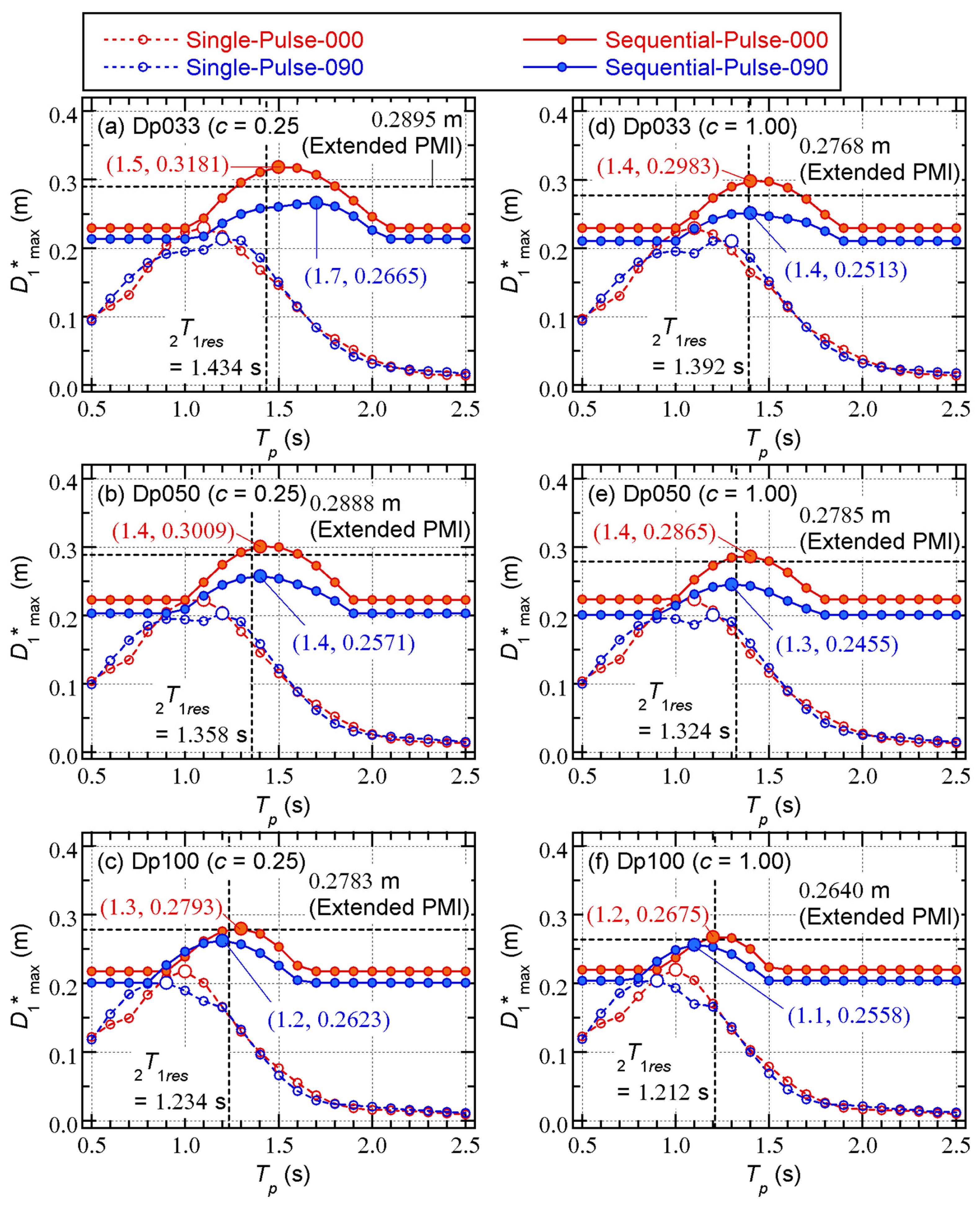
3.2.2. Sequential-Pulse Model
Figure 14 shows comparisons of the local responses ( and ) obtained from NTHA using sequential-pulse models and extended critical PMI analysis. This figure shows all the NTHA results for Sequential-Pulse-000 and Sequential-Pulse-090 along with their envelopes. “Extended PMI” in this figure consists of the envelopes of Sequential-1 and 2 in Figure 5.
The following observations can be made from Figure 14:
- The values obtained from Extended PMI agree well with the NTHA envelopes for Dp050 and Dp100. However, for Dp033, the values from Extended PMI underestimate the NTHA envelope.
- The values obtained from Extended PMI are close to the NTHA envelopes.
Figure 15 shows comparisons of the – relationship from NTHA in the sequential pulse models. For each value, the larger value obtained from NTHA using the same-sign ( = ) and opposite-sign ( = ) inputs is plotted in this figure. The values of and obtained from extended ICPMIA (Sequential-2) are shown for comparison.
The following observations can be made from Figure 15:
- The largest values obtained from NTHA are close to from extended ICPMIA. The largest value from Sequence-Pulse-000 is larger than from extended ICPMIA for all models. Meanwhile, the largest from Sequence Pulse-090 is smaller than from extended ICPMIA.
- The value of obtained from the sequential-pulse model is larger than from the single-pulse model. For model Dp033 ( = 0.25) in Figure 15a, the ratio is 1.5/1.1 = 1.36 for Sequential-Pulse-000, while is 1.7/1.2 = 1.42 for Sequential-Pulse-090. Meanwhile, for model Dp100 ( = 0.25) in Figure 15c, the ratios for Sequential-Pulse-000 and 090 are 1.2/1.0 = 1.20 and 1.1/0.9 = 1.22, respectively.
- The values of are close to from extended ICPMIA.
3.3. Discussion
The analysis results in this section can be summarized as follows:
- The ICPMIA results provide accurate approximations of the most critical local response (peak story drift and normalized cumulative strain energy of SDC damper panels) for the single-pulse models. In addition, the extended ICPMIA results accurately approximate the most critical local response for the sequential-pulse models.
- For a sequential-pulse model, the pulse-period condition < produces the most critical response for a given RC MRF model. In other words, repeating the same pulse model with the same pulse period ( = = ) will not produce the most critical response for the sequential pulsive input.
The second conclusion is consistent with the results in the previous section. That is, because the response period of the first mode in the second MI () is longer than that in the first MI(), should be longer than to produce the most critical response for a sequential input of two pulses. It should be emphasized that applying the same ground acceleration several times (the repeated approach), which has been done in many past studies, does not produce the most critical response for the earthquake sequences.
4. Conclusions
In this article, the seismic behavior of an RC MRF with SDCs under pulse-like ground motion sequences was investigated by applying an extended ICPMIA. An extended ICPMIA of RC MRF models was carried out in the first part of this study. The main conclusions from the first part can be summarized as follows:
- I)
- When the pulse velocities of the two MIs are the same in the sequential MIs, the equivalent velocities of the maximum momentary input energy of the first modal response () in both MIs are similar. The peak equivalent displacement () of an RC MRF with SDCs in sequential MIs is larger than that for a single MI when the signs of the first and second MIs are the same. This trend is notable when the SDC strength is relatively low, and the pinching behavior of RC beam is significant.
- II)
- For similar values of , the cumulative strain energy of RC members during the second MI in the sequential MIs is smaller than that for a single MI. This trend is notable when the pinching behavior of RC beam is significant. Meanwhile, the cumulative strain energy of SDCs during the second of the sequential MIs is smaller than that for a single MI when the signs of the first and second MIs are the same.
- III)
- For similar values of , the response period of the first mode in the second MI () is longer than that for a single MI. This trend is notable when the SDC strength is relatively lower, and the pinching behavior of RC beam is significant.
The second analytical study focused on the influence of the pulse period of pulse-like ground motion sequences on the response of RC MRFs with SDCs. An NTHA of RC MRF models with SDCs was carried out using the sequential pulse-like ground motion model. The main conclusions from the second part can be summarized as follows:
- I)
- In the NTHA results for sequential pulse-like ground motion, the most critical period of the second input () is longer than that of a single input ().
- II)
- The most critical response obtained from NTHA using sequential pulses can be approximated by the extended ICPMIA results.
Conclusions I) to II) answer questions 1 to 4 in Section 1.2. These conclusions support the effectiveness of the extended ICPMIA presented in the author’s previous study (Fujii, 2025a).
The significance of this study can be summarized in two points. The first is that the extended ICPMIA clearly evaluates the basic behavior of RC MRFs with SDCs subjected to an earthquake sequence. Specifically, this study has clearly evaluated the influence of the strength ratio of SDCs to RC MRF and the pinching behavior of RC beam on (a) the peak displacement of the RC MRF in a sequential seismic input, (b) degradation in hysteretic dissipated energy of RC members and SDCs during the second seismic input in the non-damaged case, and (c) the increase in natural period in the second seismic input in the non-damaged case. Unlike the results of most previous studies, the results herein are independent of the complex frequency characteristics of the selected input ground motions used in NTHA. Therefore, those presented herein represent the basic nonlinear characteristics of an RC MRF with SDCs because they are derived from the analyzed structures themselves. The second point is that the most critical response of an RC MRF with SDCs subjected to a sequential pulsive input can be approximated by the extended ICPMIA. This achievement contributes to the method of seismic design of building structures considering earthquake sequences.
Note that these results may only be valid for the RC MRF models with SDCs studied herein. Therefore, without further verification using additional building models, the following questions remain unanswered. This list is not comprehensive:
- One of the most important issues in the seismic design of an RC MRF with SDCs is evaluating the damage to RC members and SDCs. Because the damper panel in SDC is made of low-yield-strength steel, its damage evaluation may be based on the peak shear strain and the cumulative strain energy. If the proper relationship between the ultimate peak shear strain (or strain amplitude) and cumulative strain energy at failure of the damper panel is known, then it is possible to evaluate the limit of the story drift of an RC MRF when the damper panel reaches the failure. What will the story drift limit be? Will it be larger than the story drift considered in the design of an RC MRF with SDCs (e.g., 2%)? How will the number of impulsive inputs () influence the story drift limit?
- One of our previous studies (Fujii and Shioda, 2023) proposed a simplified procedure to predict the peak and cumulative responses of an RC MRF with SDCs. Because this simplified procedure is based on nonlinear static (pushover) analysis, it is much easier to apply in daily design work. However, to extend this simplified procedure to the case of an earthquake sequence, it is necessary to evaluate the − and − (or − ) relationships of RC MRFs. How can and be formulated considering the previous response of the RC MRF?
Data Availability Statement
The raw data supporting the conclusions of this article will be made available by the author without undue reservation.
Author Contributions
KF: Writing–original draft; writing–review; and editing.
Funding
This study received financial support from JSPS KAKENHI Grant Number JP23K04106.
Conflict of Interest
The author declares that the research was conducted in the absence of any commercial or financial relationships that could be construed as a potential conflict of interest.
Abbreviations
DI = double impulse
ICPMIA = incremental critical pseudo-multi-impulse analysis
MDOF = multi-degree-of-freedom
MI = multi impulse
MRF = moment-resisting frame
NTHA = nonlinear time history analysis
PDI = pseudo-double impulse
PMI = pseudo-multi impulse
RC = reinforced concrete
SDC = steel damper column
SDOF = single-degree-of-freedom
References
- Abdelnaby, A.E. Fragility curves for RC frames subjected to Tohoku mainshock-aftershocks sequences. Journal of Earthquake Engineering. 2016, 22, 902–920. [Google Scholar] [CrossRef]
- Abdelnaby, A.E.; Elnashai, A.S. Performance of degrading reinforced concrete frame systems under the Tohoku and Christchurch earthquake sequences. Journal of Earthquake Engineering. 2014, 18, 1009–1036. [Google Scholar] [CrossRef]
- Akehashi, H.; Takewaki, I. Pseudo-double impulse for simulating critical response of elastic-plastic MDOF model under near-fault earthquake ground motion. Soil Dynamics and Earthquake Engineering. 2021, 150, 106887. [Google Scholar] [CrossRef]
- Akehashi, H.; Takewaki, I. Pseudo-multi impulse for simulating critical response of elastic-plastic high-rise buildings under long-duration, long-period ground motion. The Structural Design of Tall and Special Buildings. 2022, 31, e1969. [Google Scholar] [CrossRef]
- Akehashi, H.; Takewaki, I. Bounding of earthquake response via critical double impulse for efficient optimal design of viscous dampers for elastic-plastic moment frames. Japan Architectural Review. 2022, 5, 131–149. [Google Scholar] [CrossRef]
- Akiyama, H. (1985). Earthquake resistant limit-state design for buildings. Tokyo: University of Tokyo Press.
- Akiyama, H. (1999). Earthquake-resistant design method for buildings based on energy balance. Tokyo: Gihodo Shuppan.
- Alıcı, F.S.; Sucuoğlu, H. (2024). “Input energy from mainshock-aftershock sequence during February 6, 2023 Earthquakes in South East Türkiye”, in Proceedings of the 18th World Conference on Earthquake Engineering, Milan, Italy.
- Alavi, B.; Krawinkler, H. (2000). “Consideration of near-fault ground motion effect in seismic design”, in Proceedings of the 12th World Conference on Earthquake Engineering, Auckland, New Zealand.
- Alavi, B.; Krawinkler, H. Behavior of moment-resisting frame structures subjected to near-fault ground motions. Earthquake Engineering and Structural Dynamics. 2004, 33, 687–706. [Google Scholar] [CrossRef]
- Amadio, C.; Fragiacomo, M.; Rajgelj, S. The effects of repeated earthquake ground motions on the non-linear response of SDOF system. Earthquake Engineering and Structural Dynamics. 2003, 32, 291–308. [Google Scholar] [CrossRef]
- Benavent-Climent, A.; Mollaioli, F. (eds) (2021). Energy-Based Seismic Engineering, Proceedings of IWEBSE 2021. Cham: Springer.
- Dindar, A.A.; Benavent-Climent, A.; Mollaioli, F.; Varum, H. (eds) (2025). Energy-Based Seismic Engineering, Proceedings of IWEBSE 2025. Cham: Springer.
- Di Sarno, L. Effects of multiple earthquakes on inelastic structural response. Engineering Structures. 2013, 56, 673–681. [Google Scholar] [CrossRef]
- Di Sarno, L.; Amiri, S. Period elongation of deteriorating structures under mainshock-aftershock sequences. Engineering Structures. 2019, 196, 109341. [Google Scholar] [CrossRef]
- Donaire-Ávila, J.; Galé-Lamuela, D.; Benavent-Climent, A.; Mollaioli, F. (2024). “Cumulative damage in buildings designed with energy and force methods under sequences of earthquakes”, in Proceedings of the 18th World Conference on Earthquake Engineering, Milan, Italy.
- Fujii, K. Peak and cumulative response of reinforced concrete frames with steel damper columns under seismic sequences. Buildings. 2022, 12, 275. [Google Scholar] [CrossRef]
- Fujii, K. Critical pseudo-double impulse analysis evaluating seismic energy input to reinforced concrete buildings with steel damper columns. Frontiers in Built Environment. 2024, 10, 1369589. [Google Scholar] [CrossRef]
- Fujii, K. Seismic capacity evaluation of reinforced concrete buildings with steel damper columns using incremental pseudo-multi impulse analysis. Frontiers in Built Environment. 2024, 10, 1431000. [Google Scholar] [CrossRef]
- Fujii, K. Seismic response of reinforced concrete moment-resisting frame with steel damper columns under earthquake sequences: evaluation using extended critical pseudo-multi impulse analysis. Frontiers in Built Environment. 2025, 11, 1561534. [Google Scholar] [CrossRef]
- Fujii, K. (2025), “Choice of the number of impulsive Inputs in the ICPMIA as a substitute for near-fault seismic input to RC MRFs, “in Energy-Based Seismic Engineering, Proceedings of IWEBSE 2025, Istanbul, Türkiye.
- Fujii, K.; Kanno, H.; Nishida, T. Formulation of the time-varying function of momentary energy input to a single-degree-of-freedom system using Fourier series. Journal of Japan Association for Earthquake Engineering. 2021, 21, 28–47. [Google Scholar] [CrossRef]
- Fujii, K.; Shioda, M. Energy-based prediction of the peak and cumulative response of a reinforced concrete building with steel damper columns. Buildings. 2023, 13, 401. [Google Scholar] [CrossRef]
- Galé-Lamuela, D.; Donaire-Ávila, J.; Benavent-Climent, A.; Mollaioli, F. (2025). “Damage Distribution in Buildings Under Sequences of Earthquakes, “in Energy-Based Seismic Engineering, Proceedings of IWEBSE 2025, Istanbul, Türkiye.
- Hatzigeorgiou, G.D. Behavior factors for nonlinear structures subjected to multiple near-fault earthquakes. Computers and Structures. 2010, 88, 309–321. [Google Scholar] [CrossRef]
- Hatzigeorgiou, G.D. Ductility demand spectra for multiple near-and far-fault earthquakes. Soil Dynamics and Earthquake Engineering. 2010, 30, 170–183. [Google Scholar] [CrossRef]
- Hatzigeorgiou, G.D.; Beskos, D.E. Inelastic displacement ratios for SDOF structures subjected to repeated earthquakes. Engineering Structures. 2009, 31, 2744–2755. [Google Scholar] [CrossRef]
- Hatzigeorgiou, G.D.; Liolios, A.A. Nonlinear behaviour of RC frames under repeated strong ground motions. Soil Dynamics and Earthquake Engineering. 2010, 30, 1010–1025. [Google Scholar] [CrossRef]
- Hori, N.; Inoue, N. Damaging properties of ground motion and prediction of maximum response of structures based on momentary energy input. Earthquake Engineering and Structural Dynamics. 2002, 31, 1657–1679. [Google Scholar] [CrossRef]
- Katayama, T.; Ito, S.; Kamura, H.; Ueki, T.; Okamoto, H. (2000). “Experimental study on hysteretic damper with low yield strength steel under dynamic loading,” in Proceedings of the 12th World Conference on Earthquake Engineering, Auckland, New Zealand.
- Kojima, K.; Takewaki, I. (2015a). Critical earthquake response of elastic–plastic structures under near-fault ground motions (Part 1: Fling-step input). Frontiers in Built Environment. 1, 12.
- Kojima, K.; Takewaki, I. (2015b). Critical earthquake response of elastic–plastic structures under near-fault ground motions (Part 2: Forward-directivity input). Frontiers in Built Environment. 1, 13.
- Kojima, K.; Takewaki, I. (2015c). Critical input and response of elastic–plastic structures under long-duration earthquake ground motions. Frontiers in Built Environment. 1, 15.
- Mahin, A. (1980). “Effect of duration and aftershock on inelastic design earthquakes,” in Proceedings of the 9th World Conference on Earthquake Engineering, Istanbul, Turkey.
- Mavroeidis, G.P.; Papageorgiou, A.S. A Mathematical Representation of Near-Fault Ground Motions. Bulletin of the Seismological Society of America. 2003, 93, 1099–1131. [Google Scholar] [CrossRef]
- Mavroeidis, G.P.; Dong, G.; Papageorgiou, A.S. Near-fault ground motions, and the response of elastic and inelastic single-degree-of-freedom (SDOF) systems. Earthquake Engineering and Structural Dynamics. 2004, 33, 1023–1049. [Google Scholar] [CrossRef]
- Muto, K.; Hisada, T.; Tsugawa, T.; Bessho, S. (1974). “Earthquake resistant design of a 20 story reinforced concrete buildings” in Proceedings of the fifth world conference on earthquake engineering, Rome, Italy.
- Ono, Y.; Kaneko, H. (2001). “Constitutive rules of the steel damper and source code for the analysis program,” in Proceedings of the Passive Control Symposium 2001, Yokohama, Japan (In Japanese).
- Otani, S. Hysteresis models of reinforced concrete for earthquake response analysis. Journal of the Faculty of Engineering the University of Tokyo. 1981, 36, 125–156. [Google Scholar]
- Ruiz-García, J.; Negrete-Manriquez, J.C. Evaluation of drift demands in existing steel frames under as-recorded far-field and near-fault mainshock–aftershock seismic sequences. Engineering Structures 2011, 33, 621–634. [Google Scholar] [CrossRef]
- Ruiz-García, J. Mainshock-Aftershock Ground Motion Features and Their Influence in Building’s Seismic Response. Journal of Earthquake Engineering. 2012, 16, 719–737. [Google Scholar] [CrossRef]
- Ruiz-García, J. (2013). “Three-dimensional building response under seismic sequences,” in Proceedings of the 2013 World Congress on Advances in Structural Engineering and Mechanics (ASEM13), Jeju, Korea.
- Takewaki, I. Review: Critical Excitation Problems for Elastic–Plastic Structures Under Simple Impulse Sequences. Japan Architectural Review. 2025, 8, e70037. [Google Scholar] [CrossRef]
- Takewaki, I.; Kojima, K. (2021). An Impulse and Earthquake Energy Balance Approach in Nonlinear Structural Dynamics. Boca Raton, FL: CRC Press.
- Uang, C.; Bertero, V.V. Evaluation of seismic energy in structures. Earthquake Engineering and Structural Dynamics. 1990, 19, 77–90. [Google Scholar] [CrossRef]
- Varum, H.; Benavent-Climent, A.; Mollaioli, F. (eds) (2023). Energy-Based Seismic Engineering, Proceedings of IWEBSE 2023. Cham: Springer.
- Wada, A.; Huang, Y.; Iwata, M. Passive damping technology for buildings in Japan. Progress in Structural Engineering and Materials. 2000, 2, 335–350. [Google Scholar] [CrossRef]
- Xu, Z.; Agrawal, A.K.; He, W.L.; Tan, P. Performance of passive energy dissipation systems during near-field ground motion type pulses. Engineering Structures 2007, 29, 224–236. [Google Scholar] [CrossRef]
- Yaghmaei-Sabegh, S. Time–frequency analysis of the 2012 double earthquakes records in North-West of Iran. Bulletin of Earthquake Engineering. 2014, 12, 585–606. [Google Scholar] [CrossRef]
- Yaghmaei-Sabegh, S.; Ruiz-García, J. Nonlinear response analysis of SDOF systems subjected to doublet earthquake ground motions: A case study on 2012 Varzaghan–Ahar events. Engineering Structures. 2016, 110, 281–292. [Google Scholar] [CrossRef]
- Yang, F.; Wang, G.; Ding, Y. Damage demands evaluation of reinforced concrete frame structure subjected to near-fault seismic sequences. Natural Hazards. 2019, 97, 841–860. [Google Scholar] [CrossRef]
- Zhai, C.; Ji, D.; Wen, W.; Lei, W.; Xie, L.; Gong, M. The inelastic input energy spectra for main shock–aftershock sequences. Earthquake Spectra 2016, 32, 2149–2166. [Google Scholar] [CrossRef]
Figure 1.
Extended Critical PMI Analysis.
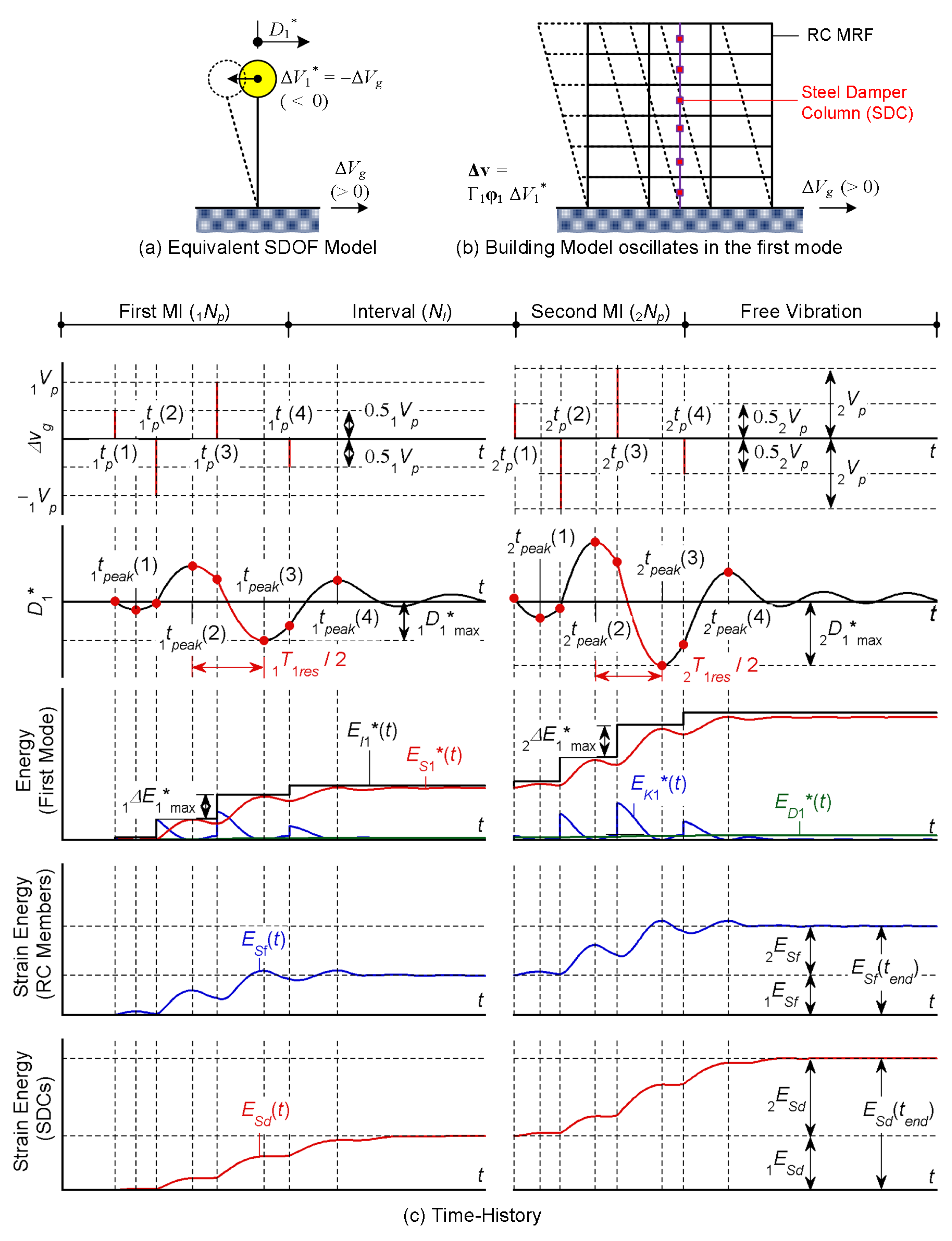
Figure 2.
Building Model.
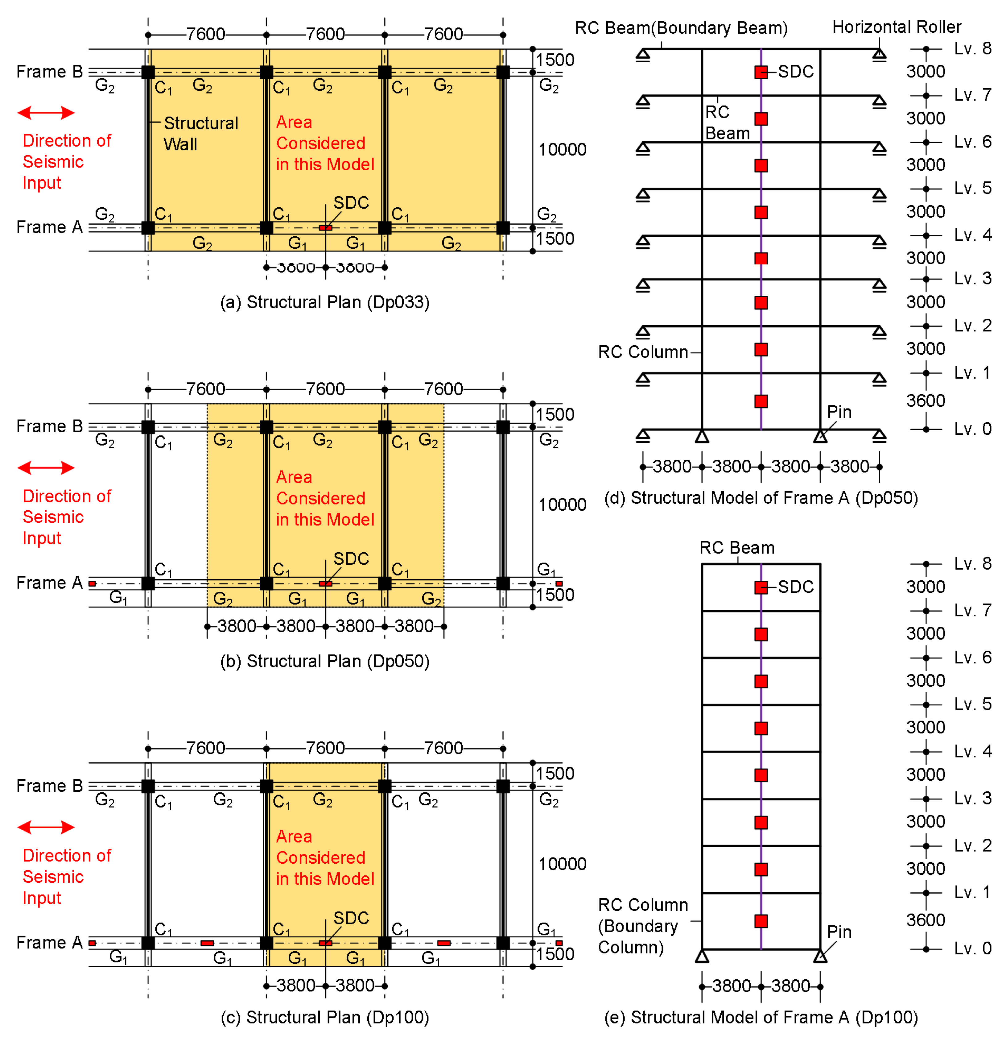
Figure 3.
Hysteresis Model.
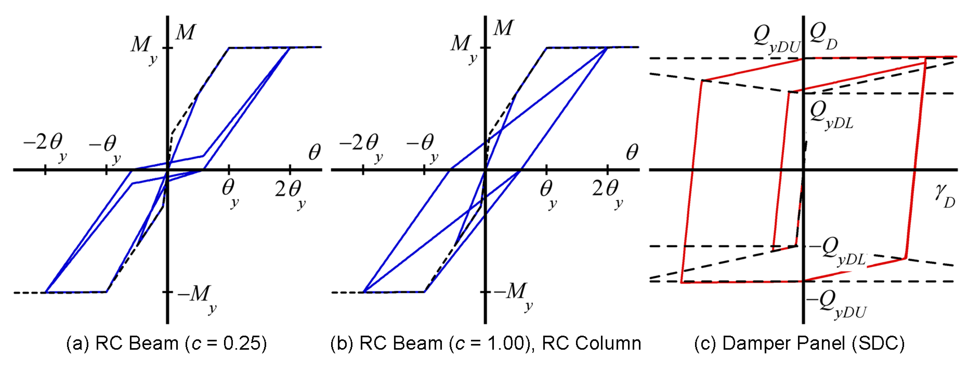
Figure 4.
Comparisons of the VΔE1* – D1*max relationship and the VΔE1* – Vp relationship in case of a single MI.
Figure 4.
Comparisons of the VΔE1* – D1*max relationship and the VΔE1* – Vp relationship in case of a single MI.
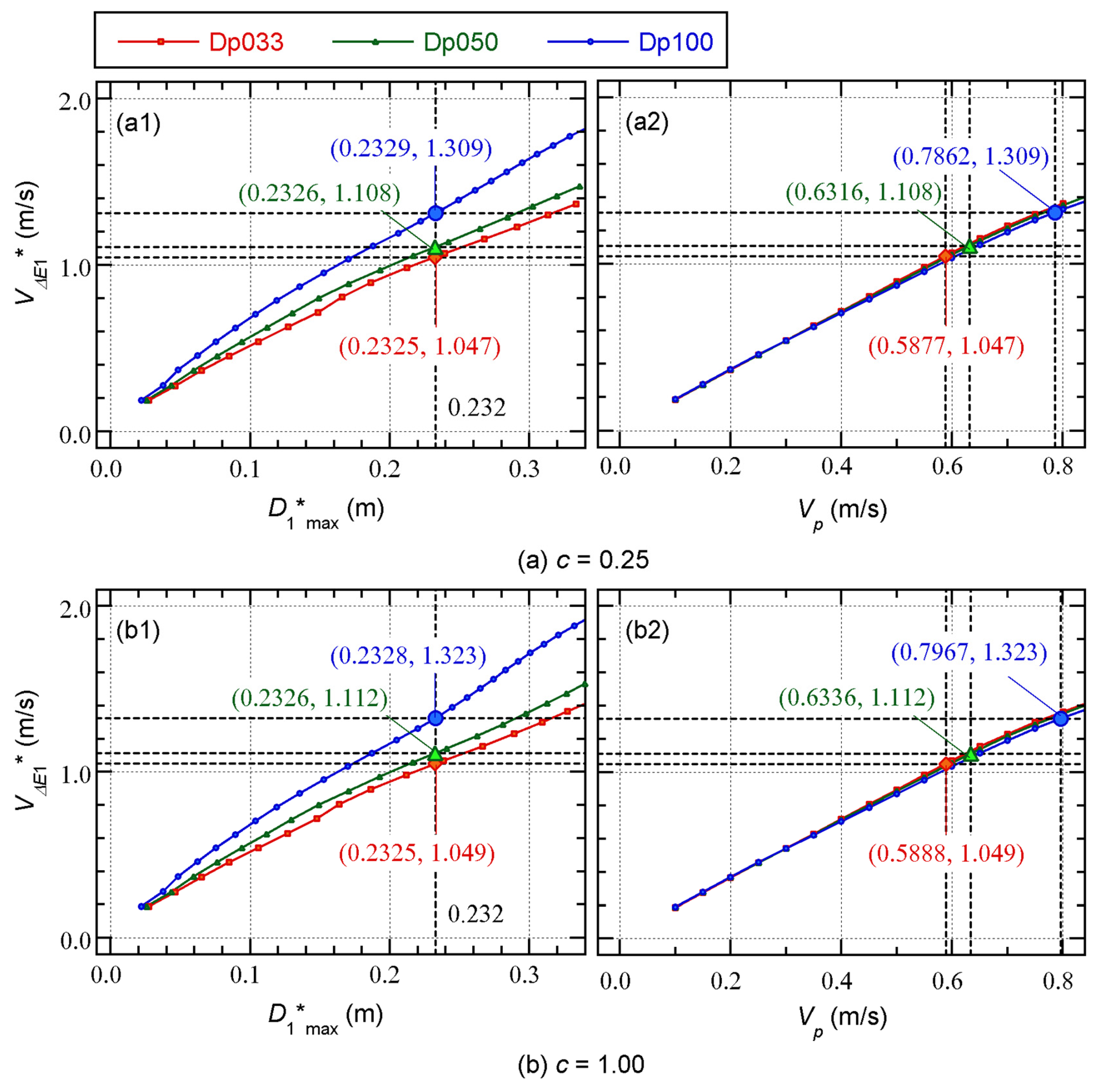
Figure 5.
Comparisons of the local responses obtained from extended critical PMI analyses in case of 2Vp = 1Vp.
Figure 5.
Comparisons of the local responses obtained from extended critical PMI analyses in case of 2Vp = 1Vp.
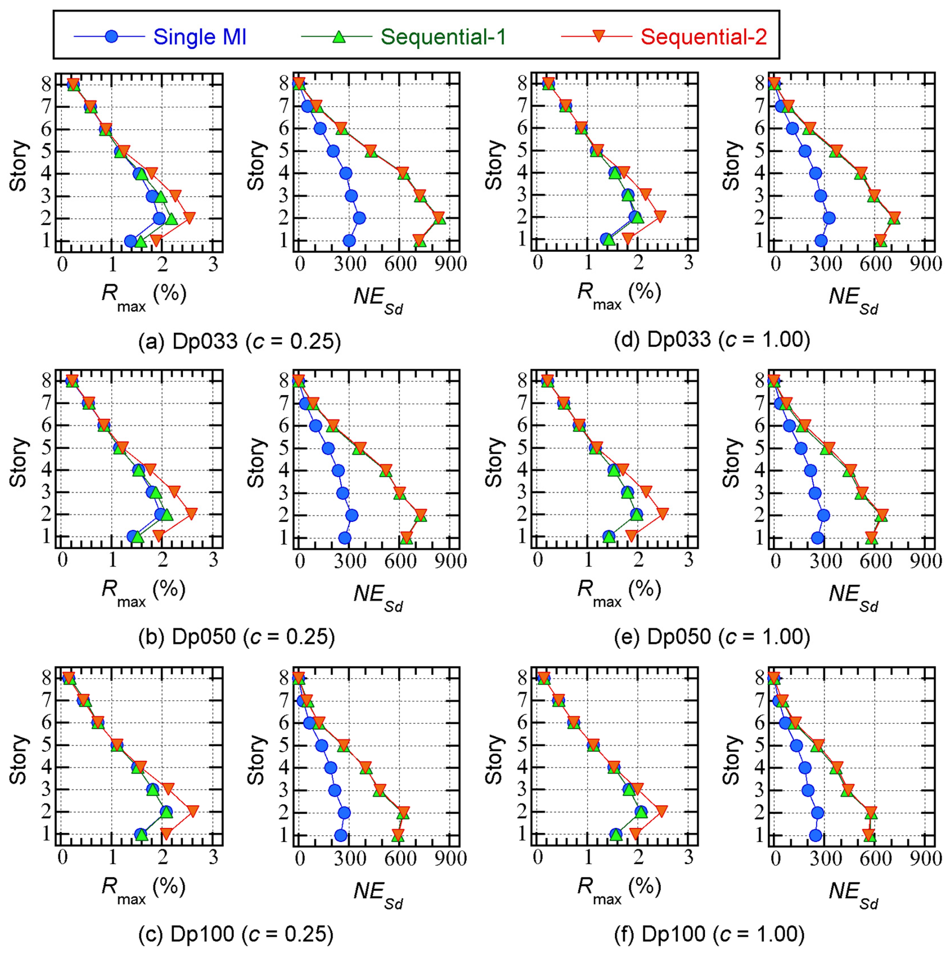
Figure 6.
Hysteresis Loop obtained from extended critical PMI analysis in case of 2Vp = 1Vp.
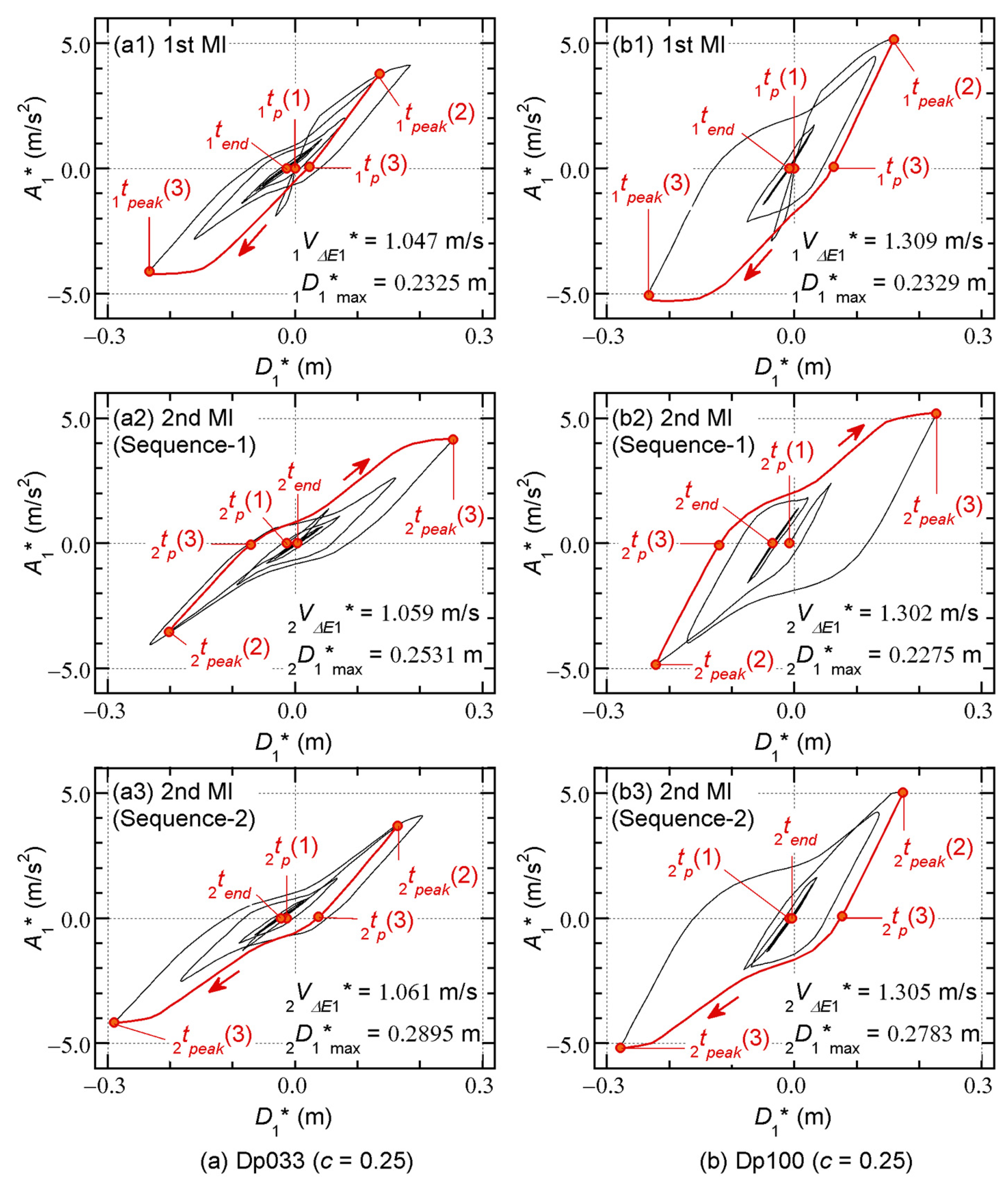
Figure 7.
Comparisons of the VΔE1* – D1*max relationship.
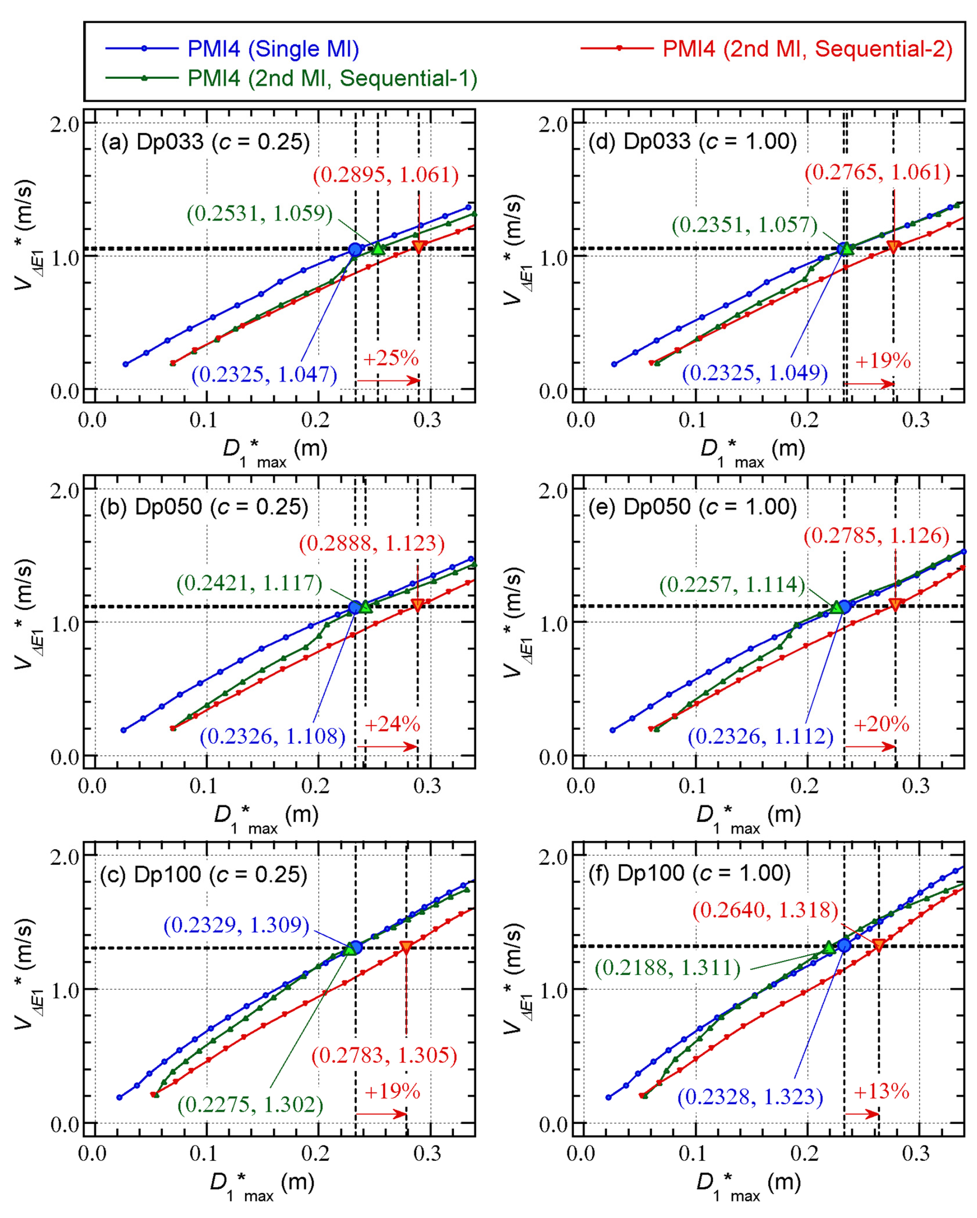
Figure 8.
Comparisons of the VΔE1* – T1res relationship.
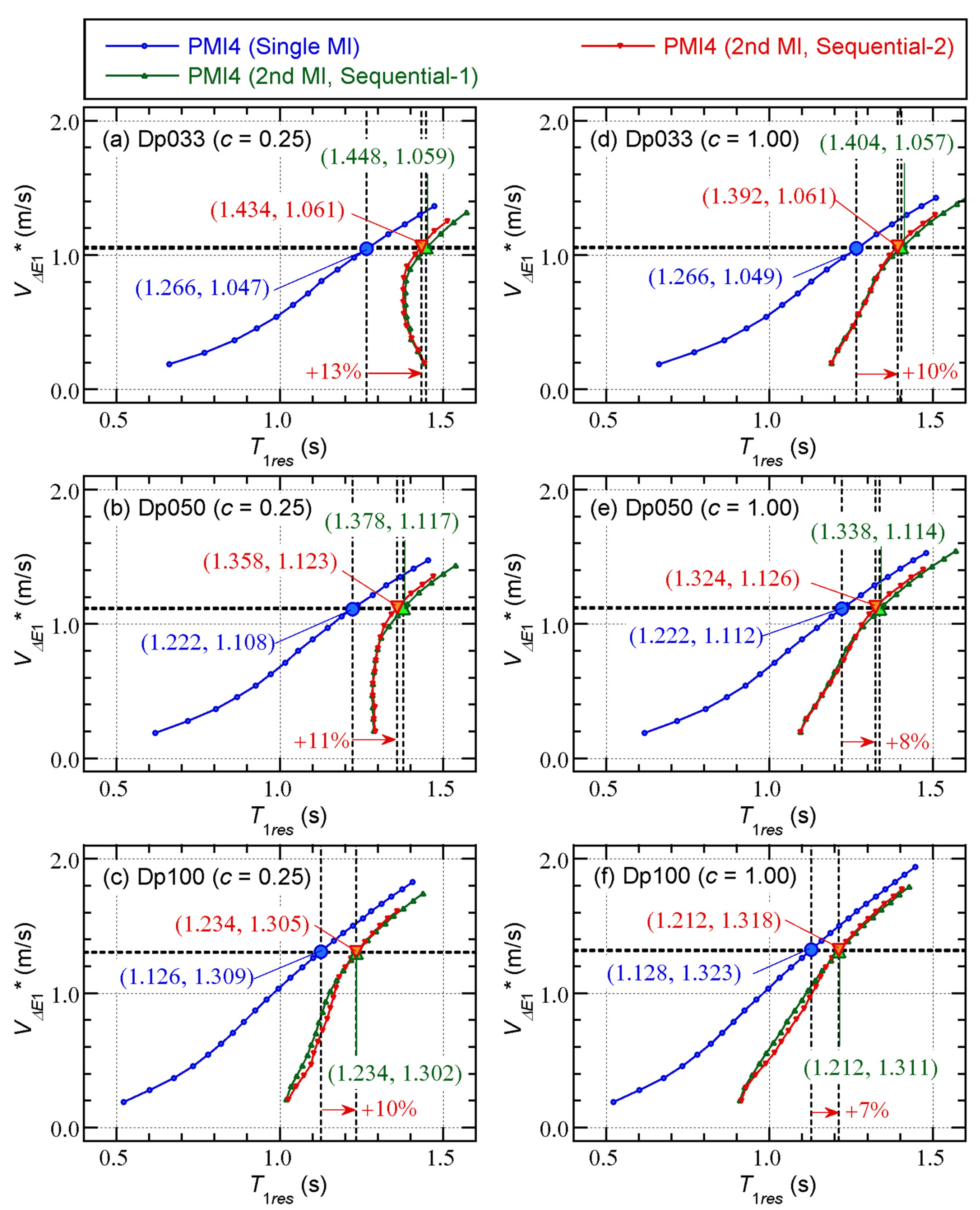
Figure 9.
Comparisons of the ESf / M – D1*max relationship.
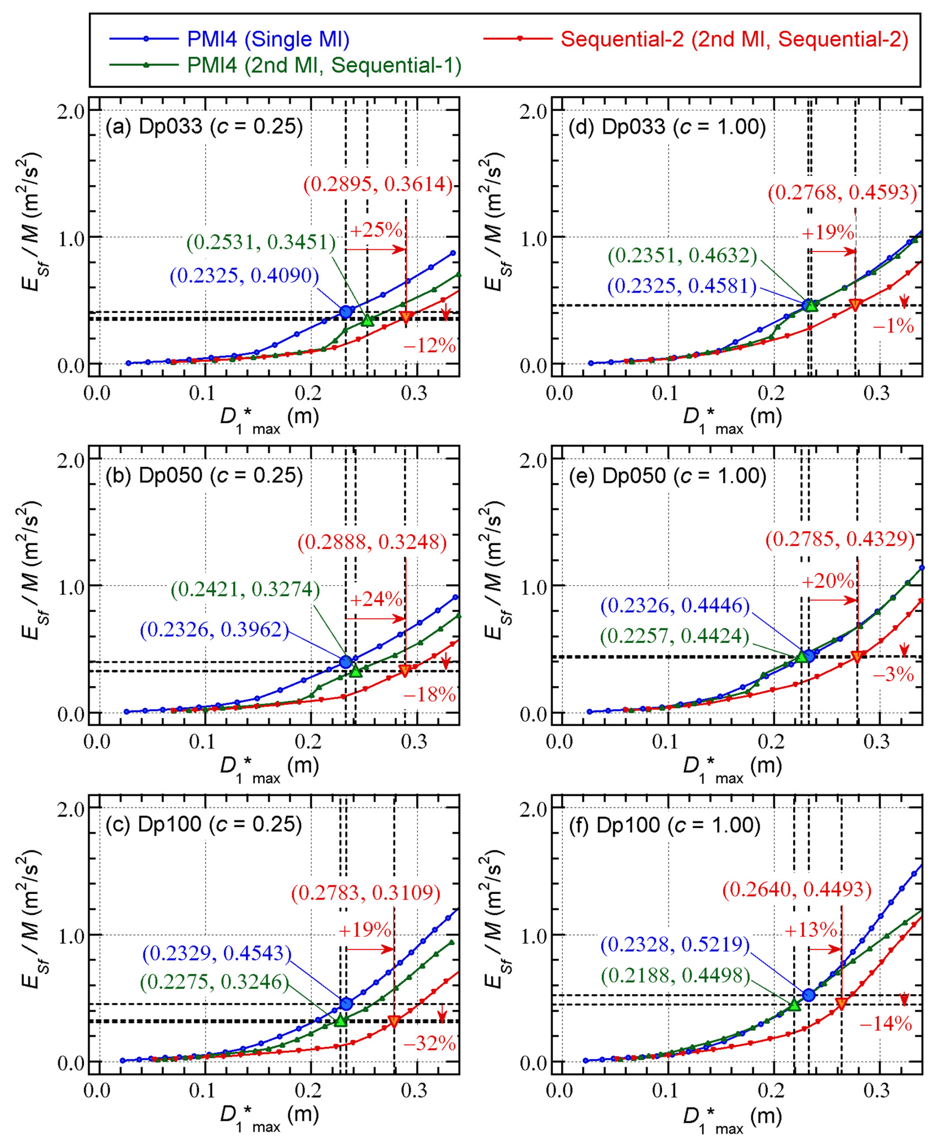
Figure 10.
Comparisons of the ESd / M – D1*max relationship.
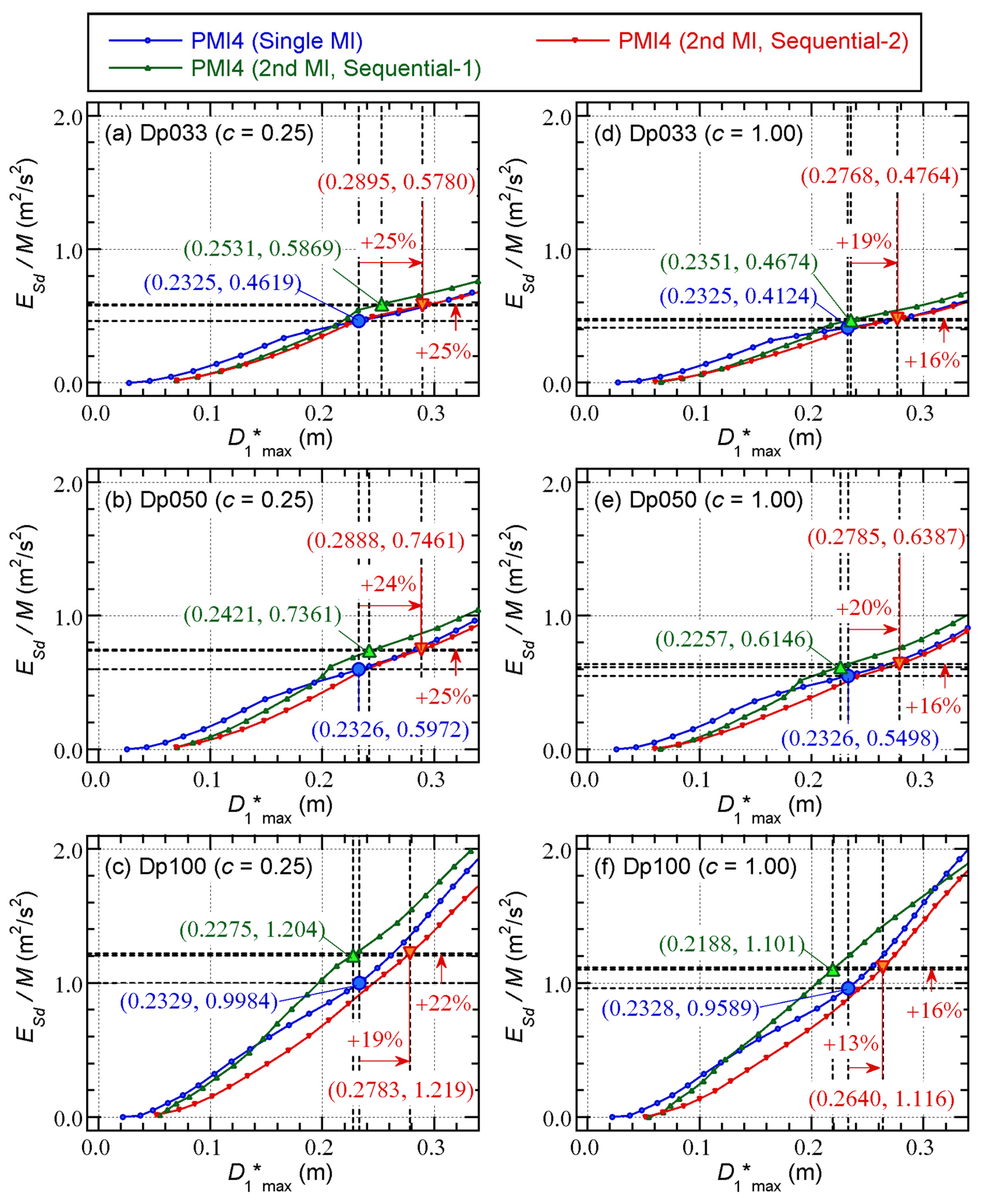
Figure 11.
Pulse-like ground motion model.
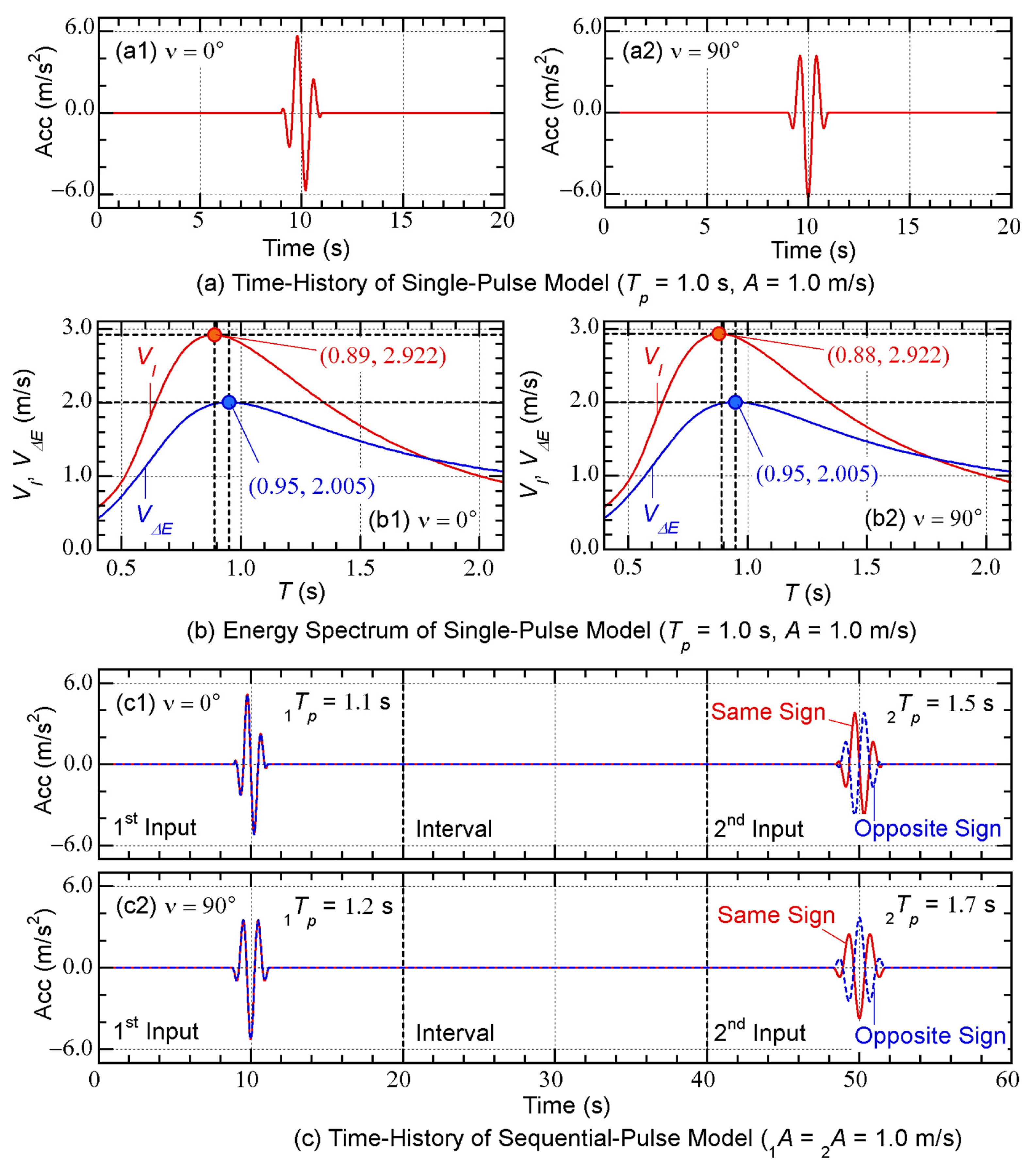
Figure 12.
Comparisons of the local responses (single-pulse model).
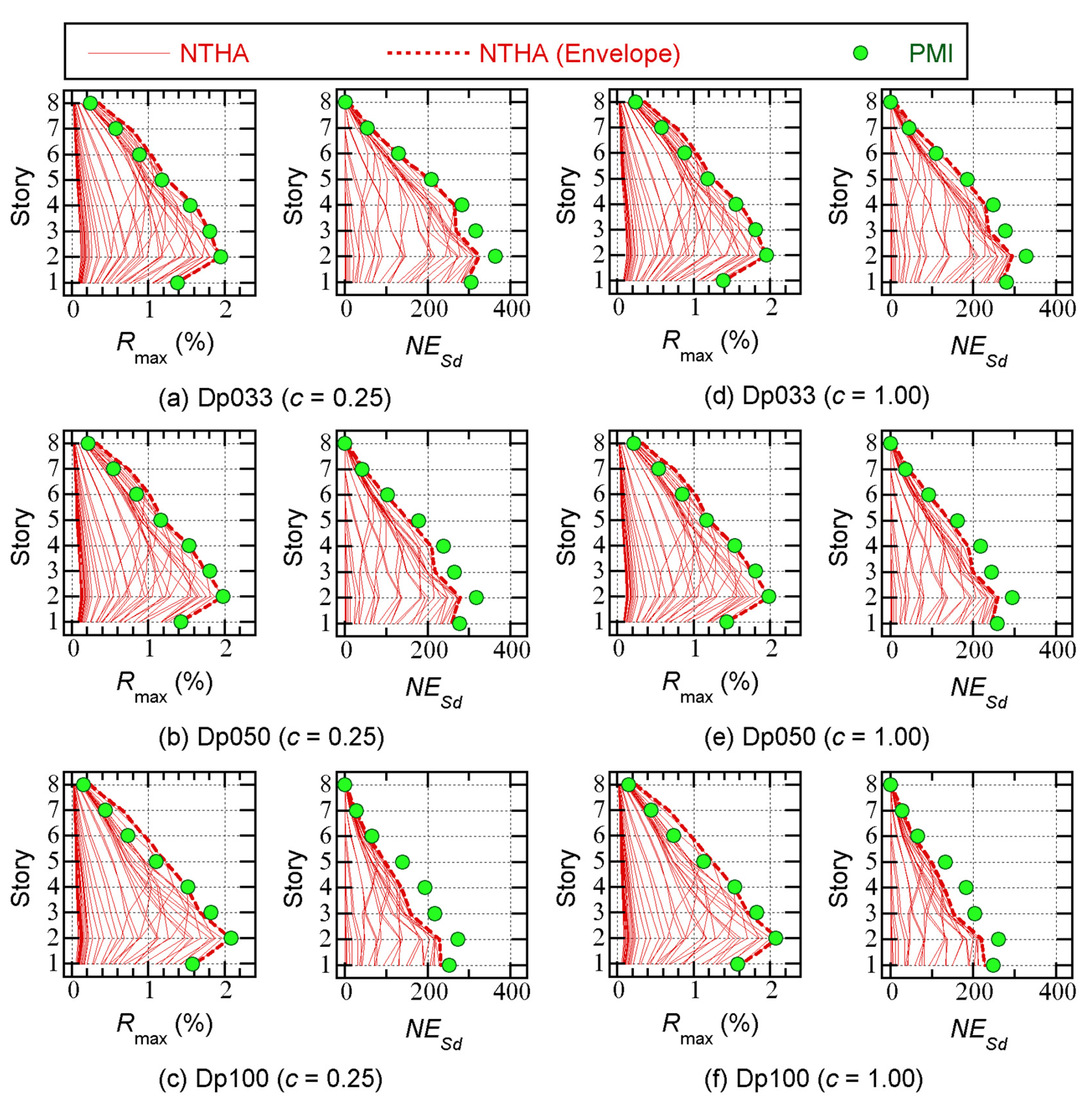
Figure 13.
Comparisons of the D1*max – Tp relationship (single-pulse model).
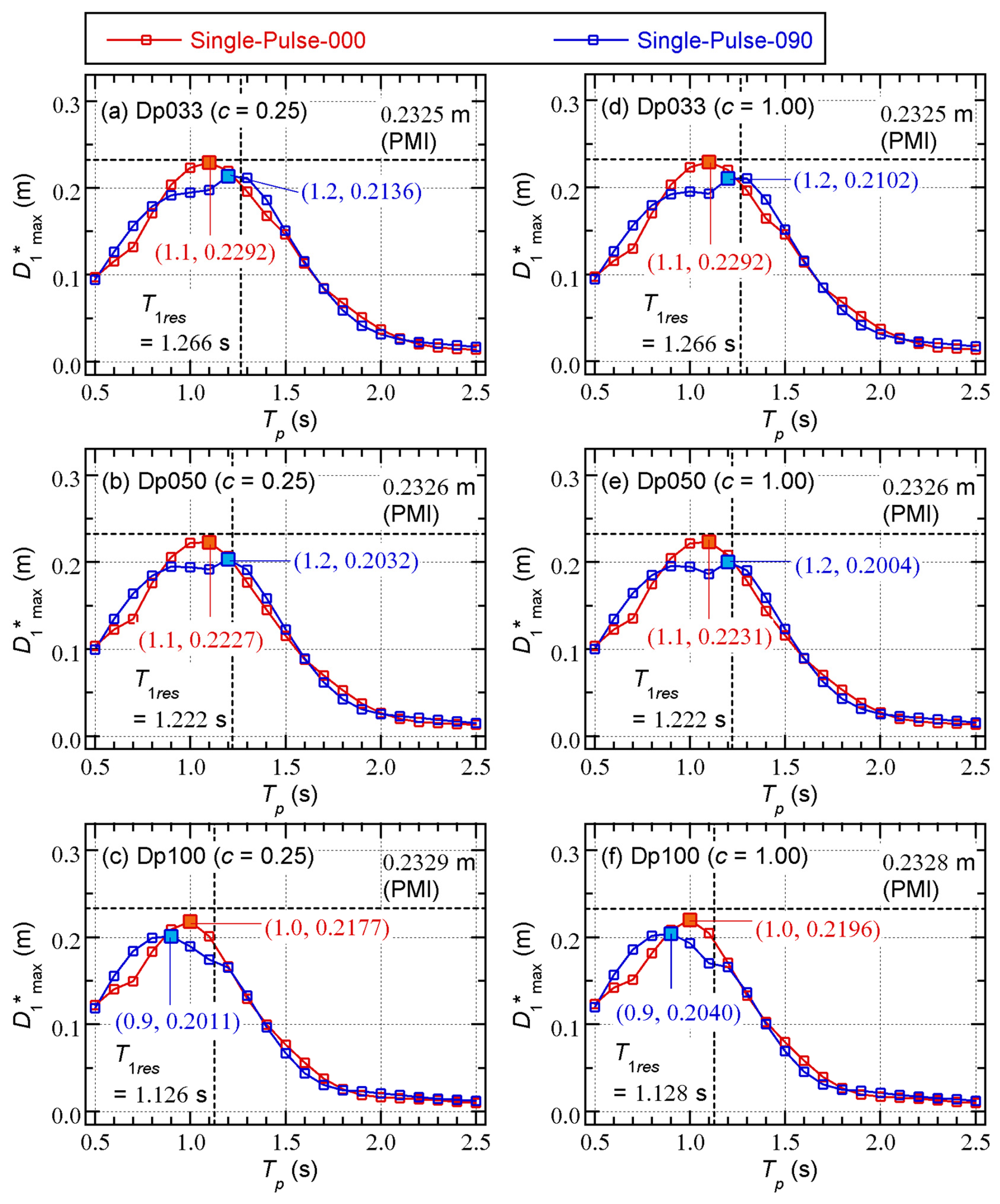
Figure 14.
Comparisons of the local responses (sequential-pulse model).
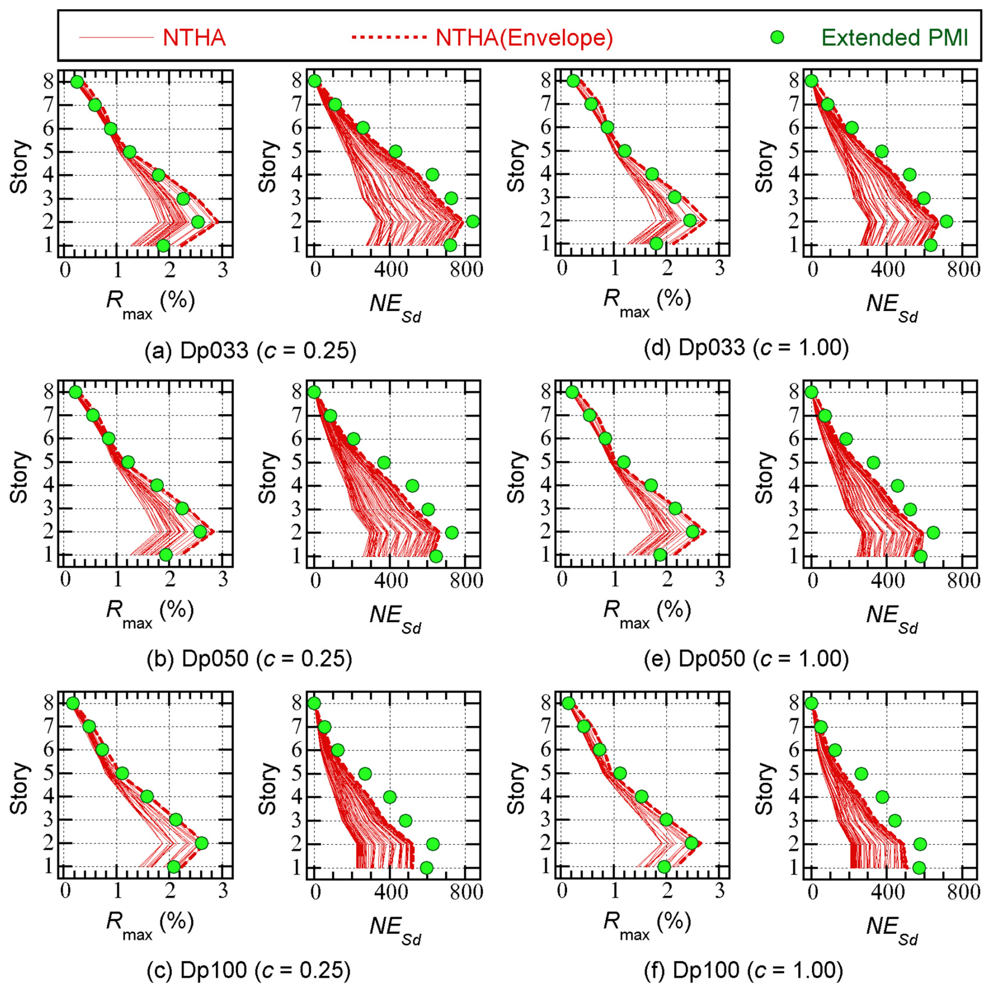
Figure 15.
Comparisons of the D1*max – Tp relationship (sequential-pulse model).
Disclaimer/Publisher’s Note: The statements, opinions and data contained in all publications are solely those of the individual author(s) and contributor(s) and not of MDPI and/or the editor(s). MDPI and/or the editor(s) disclaim responsibility for any injury to people or property resulting from any ideas, methods, instructions or products referred to in the content. |
© 2025 by the authors. Licensee MDPI, Basel, Switzerland. This article is an open access article distributed under the terms and conditions of the Creative Commons Attribution (CC BY) license (http://creativecommons.org/licenses/by/4.0/).
Copyright: This open access article is published under a Creative Commons CC BY 4.0 license, which permit the free download, distribution, and reuse, provided that the author and preprint are cited in any reuse.


