Submitted:
21 August 2025
Posted:
21 August 2025
You are already at the latest version
Abstract
A mathematical model of high-frequency geoacoustic emission for a single dislocation radiation source is suggested in the papper. The mathematical model is a linear Berlage oscillator with non-constant coefficients whose solution is the Berlage function momentum. Further, the values of the parameters of the Berlage pulse are specified using experimental data. For this purpose, the problem of multidimensional optimization is solved, which consists of two stages: global optimization using the differential evolution method and local optimization according to the Nelder-Mead method. Statistics are given to confirm the correctness of the obtained results: standard error and coefficient of determination. It is shown that two-stage multivariate optimization makes it possible to refine the parameters of the Berlage pulse with a sufficiently high accuracy to describe high-frequency geoacoustic emission.
Keywords:
high-frequency geoacoustic emission
; Berlage pulse
; Berlage oscillator
; mathematical model
; multidimensional optimization
; differential evolution method
; Nelder-Meade method
1. Introduction
Acoustic emission in rocks (geoacoustic emission or GAE) occurs as a result of their deformation and is accompanied by the radiation of elastic sound waves, which are recorded by acoustic receivers [1]. The increased interest in the study of GAE worldwide can be explained by several important tasks related to the study of dangerous man-made and natural phenomena, such as rock bursts in mines [2], rock failure in geotechnical construction [3], landslides [4] and seismic activity in seismically hazardous regions [1]. Additionally, particular attention deserves tasks related to studying the influence of GAE on other geophysical fields [6]. On the Kamchatka Peninsula, in the area of the Petropavlovsk-Kamchatsky geodynamic testing site, GAE signals are recorded in the high-frequency range (up to the first tens of kilohertz). The importance of recording such signals is associated with studying the stress-strain state of the geological medium, which causes anomalies in GAE. In most cases, these anomalies precede seismic events — earthquakes. For example, the article [1,5] showed that in half of the cases, anomalies of high-frequency GAE in near-surface sedimentary rocks preceded strong seismic events within in the 1–3 day interval. Therefore, high-frequency GAE can be considered an operational precursor of earthquakes.
To effectively study the stressed-deformed state of geo-environments with high-frequency GAE, it is necessary to develop its mathematical models. In the theoretical work [7,8] a mathematical model was proposed on the basis of two related linear oscillators with non-constant coefficients which described the linear interaction between two dislocation sources (Belage pulses). The quantitative and qualitative properties of the mathematical model were investigated. However, the modelling results were not compared with experimental data.
In this paper, a mathematical model (Belage oscillator) will be constructed for one source of dislocations, the parameters of which are refined using experimental data obtained at the observation point of the Institute of Cosmophysical Research and Radio Wave Propagation of the Far Eastern Branch of the Russian Academy of Sciences (IKIR FEB RAS) in Kamchatka. For this purpose, we will solve the problem of multidimensional two-step optimization using differential evolution methods [9] and Nelder-Mida [10]. The work shows that the proposed algorithms allow to efficiently refine the values of key parameters of the proposed model.
The structure of the study in the article consists of the following sections: the introduction gives a description of the object of research and indicates the relevance of the selected topic (section 1). Section 2 describes the registration of GAE in Kamchatka and provides information on acoustic receivers. Section 3 provides a mathematical description of the Belage oscillator for high-frequency GAE research, as well as a description of the two-step multidimensional optimization method. In section 4, the results of the application of the multidimensional two-step optimization method are shown, the visualization of the simulation results is carried out, as well as the table of the updated values of the Belage oscillator.
2. GAE Recording Methodology
Analysis of the dynamics of geoacoustic emission pulses in the final stages of preparation of seismic events is of great interest for the identification of earthquake precursors, which is confirmed by multi-year observations of IKIR FEB RAS conducted since 1999 [11,16,17].
Geoacoustic signals of the kilohertz frequency range are generated by sources located in a rock volume limited to the semisphere radius m [7]. The diagram of the process for recording geoacoustic emission signals is shown in the figure.
The methodology for recording geoacoustic emissions in Kamchatka is based on the use of specialized acoustic receivers – piezoelectric sensors of various types. The main element of the registration system – broadband hydrophones with a frequency range of 20 Hz-20 kHz, installed on the bottom of natural and artificial water bodies (Figure 1) [18].
For recording low-frequency oscillations (0.2-400 Hz) a combined receiver is used, which consists of a three-component vertical receiver and hydrophone (Figure 2b) [13]. The three-component receiver is mounted on the end surface of the optical strainer. The feature of its installation is the spatial orientation, in which the Z-component coincides with the axis of the gauge measurement, and the X-component is directed vertically.
For high-frequency measurements, a system of four cylindrical membrane-type hydrophones with a diameter of 65 mm (Figure 1c), placed in cubic artificial water bodies ( m3) with vertical orientation is used. The three hydrophones (№2-4) form an equilateral triangle with a length of 5 m around the reflector tensometry attachment, and the fourth one (№1) is located 50 m from the central point [11,12]. Constructively, each receiver is a metal body with piezoelement, consisting of 8 rings made of piezoceramic CTBS-3 (dimensions mm), indented on the rod. On one side the rod is rigidly fixed in the body, on the other – connected to a membrane that receives acoustic pressure. This design provides high sensitivity and measurement reliability over a wide frequency range [14,15]. The signals are digitized with a sampling rate of 44.1 kHz. The output files have a flac format lasting 15 minutes.
GAE signal is characterized by a sequence of relaxation pulses of different amplitude and duration with frequency of filling from hundreds of hertz to tens of kilohertz. The frequency of repetition in calm periods is one per second, and during anomalies preceding seismic events it reaches tens or hundreds per second.
An example of recording of high-frequency geoacoustic emission data at the observation point <<Karimshina>> (52.83 N, 158.13 E) in Kamchatka located in the seismotectonic fault zone from 24 June to 27 June 2017 is on Figure 3. June 27, 2017 02:23 UTC there was an earthquake with a magnitude of 5.3 depth 40.5 km in the Pacific (52.58 N, 160.8 E) of Kamchatka. An analysis of geoacoustic emission data recorded within 72 hours prior to the seismic event revealed statistically significant changes in acoustic signal parameters indicating earthquake preparedness (Figure 3). There is an increase of the average amplitude by 35-40% compared to the background level, a more dense time distribution (reduction of intervals between pulses).
On the Figure 4a you can see that 2 days before the earthquake (25.06) pulse activity already exceeded background values, but had a more chaotic nature without a clear temporal structure. For 48 hours the appearance of individual high-amplitude pulses is observed, and for 36 hours — the frequency of pulses and the growth of their amplitude. In the 24 hours prior to the earthquake, 259747 geoacoustic emission pulses were analyzed and 63301 pulses (24.4%) similar in shape on Berlage functions were identified.
Next in the article we will use the geo-acoustic impulses given in the figure 4b-e to specify the values of key parameters of the mathematical model (functions) of Berlage.
3. Mathematical Model of GAE
For the analytical description of seismic acoustic oscillations in seismic exploration, the formulas N.N. Bubbles (Gaussian pulses) and G.P. Berlage [18,19] are widely used. In the work [18] to improve the quality of approximations of geoacoustic signals, a methodology was proposed that includes both Berlage and Gauss functions. It has been shown that this technique allows to create compact, diluted representations of geoacoustic emission signals (5-6 non-zero expansion coefficients) with a permissible error of no more than [20].
In this paper we use the following mathematical model to describe a single GAE pulse [7]:
where — pulse amplitude, from. units; — parameter responsible for signal envelope shape; — maximum position; — signal envelope slope; — time, c; — start time, s; — pulse duration, c; — fill frequency, Hz; — initial phase; ; ; ; .
The mathematical model (1), whose solution is the Berlage function (2), we will call the Berlage oscillator.
The Berlage oscillator (1) describes one dislocation source (crack) emitting one pulse of a high-frequency GAE. The articles [7,8] described the interaction of two dislocation sources using two linearly connected Berlage oscillators. Taking into account more than two dislocation sources leads us to a chain of connected Berlage oscillators, which is equivalent to considering the wave process of GAE propagation.
In this article, we will refine the parameters of the Berlage oscillator (1) using multidimensional optimization taking into account the experimental data of the GAE obtained at the observation point of the IKIR FEB RAS (Figure 4b-e). The refined values were compared with parameter values according to work results [16].
The multidimensional optimization method included two steps: the differential evolution method [9,22] and the Nelder-Mead method [10].
Differential evolution occupies a special place among modern methods of machine learning as one of the most effective optimization algorithms. This population method, belonging to the class of evolutionary algorithms, demonstrates high performance in solving complex optimization tasks. For evolutionary algorithms of scaled disturbance, the method uses a specific recombination of vectors. The algorithm consistently compares the quality of new solutions with current ones, keeping only the most effective options in the population, which ensures its high consistency and reliability when working with multidimensional search spaces [23].
The Nelder-Mead method (deformable polyhedron method, simplex method) is used for local tuning, that is, to find the local extremum of a function in several variables. The main essence of the method for optimizing functions is to successively move and deform a simplex around an extremum point. Simplex is a polyhedron of vertices in n measurements, where each point is a set of parameter values of the optimized function. The method does not use a derivative (gradients) function, so it is applicable to uneven and/or noisy functions.
In the first stage of solving the problem of multidimensional optimization, the method of differential evolution is used, and in the second stage the found values of parameters of the model (1) are adjusted using the Nelder-Mida method.
4. Research Results
The algorithms of the multidimensional optimization methods described above, as well as the visualization of the results, were implemented in the Python programming language.
The initial parameter values for the Berlage function (2) were first set according to the work [16]: , , , , , then refined using multidimensional two-stage optimization. The time interval for the pulses is selected according to the time interval of the experimental pulses (Figure 4b-e).
Analysis of the results of refinement of parameters of mathematical model (1) for geoacoustic pulses (Figure 4b-e) is shown in Figure 5, Figure 6 and Figure 7.
Figure 5a for the pulse June 27, 2017 02:22:08 clearly shows that although the model as a whole reproduces the shape of the pulse, there are minor discrepancies: the phase of amplitude increase in the experiment occurs faster than the model predicts, and the attenuation process is accompanied by additional oscillations. Spectral analysis in figure 5b shows a clear dominant peak at 3059.8 Hz.
The graph (Figure 5c) shows non-closed phase trajectories that have the shape of spirals. First, the spiral begins to unwind, while the amplitude of vibrations increases until some point in time (Figure 5a). Then the spiral begins to twist and the amplitude of the oscillations slowly decays.
The optimized model (blue line) (Figure 5d) replicates the experimental pulse form (black line) much better than the initial model. The mean squared error (MSE) decreased by 96.41%. The coefficient of determination confirms that the model explains 66.23% dispersion of data.
Figure 6.
Comparison of model impulse and experimental June 26, 2017 at 2:15:014 s.; (a) comparison of pulse amplitudes; (b) pulse spectra; (c) phase trajectories of pulses; (d) comparison with initial model.
Figure 6.
Comparison of model impulse and experimental June 26, 2017 at 2:15:014 s.; (a) comparison of pulse amplitudes; (b) pulse spectra; (c) phase trajectories of pulses; (d) comparison with initial model.
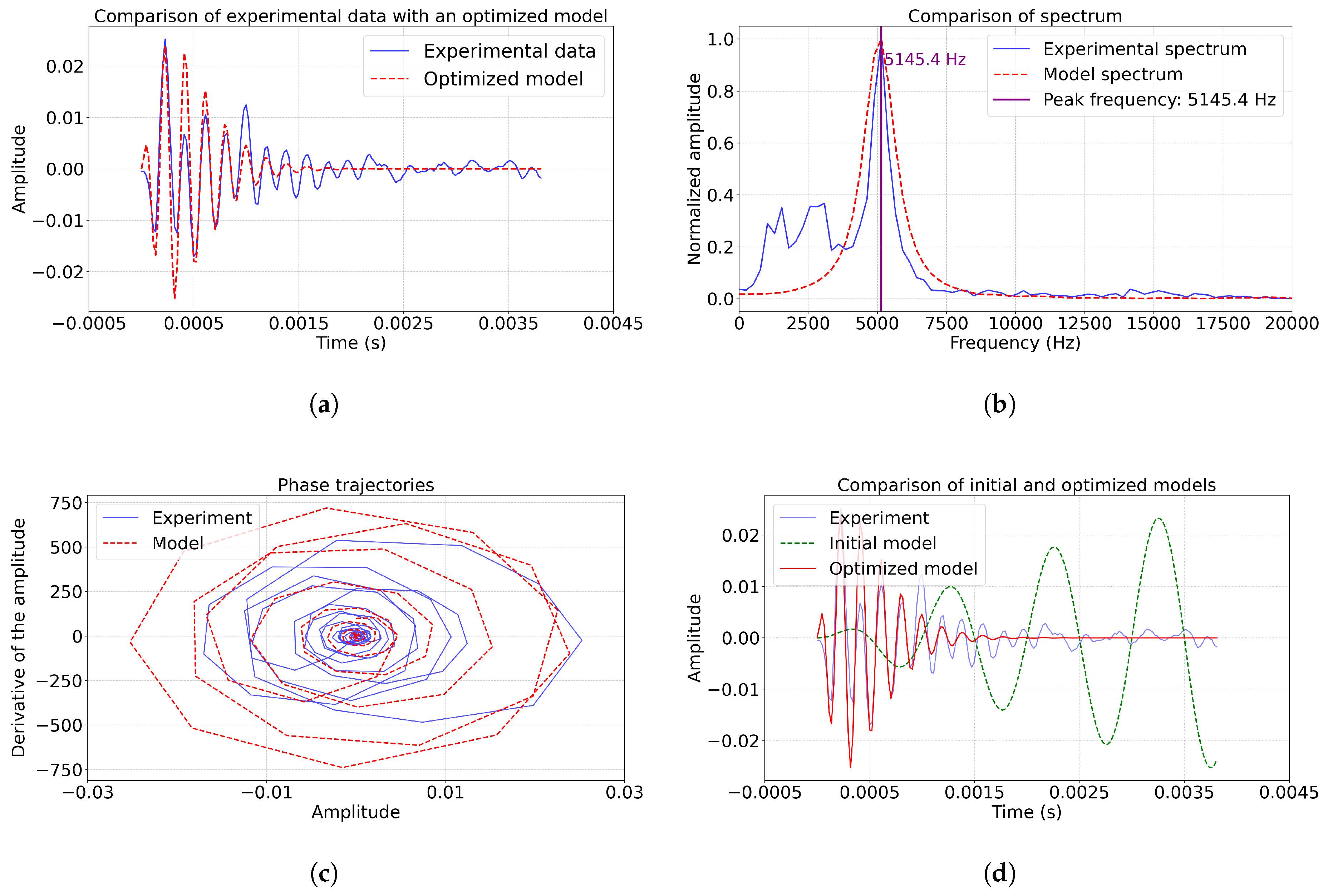
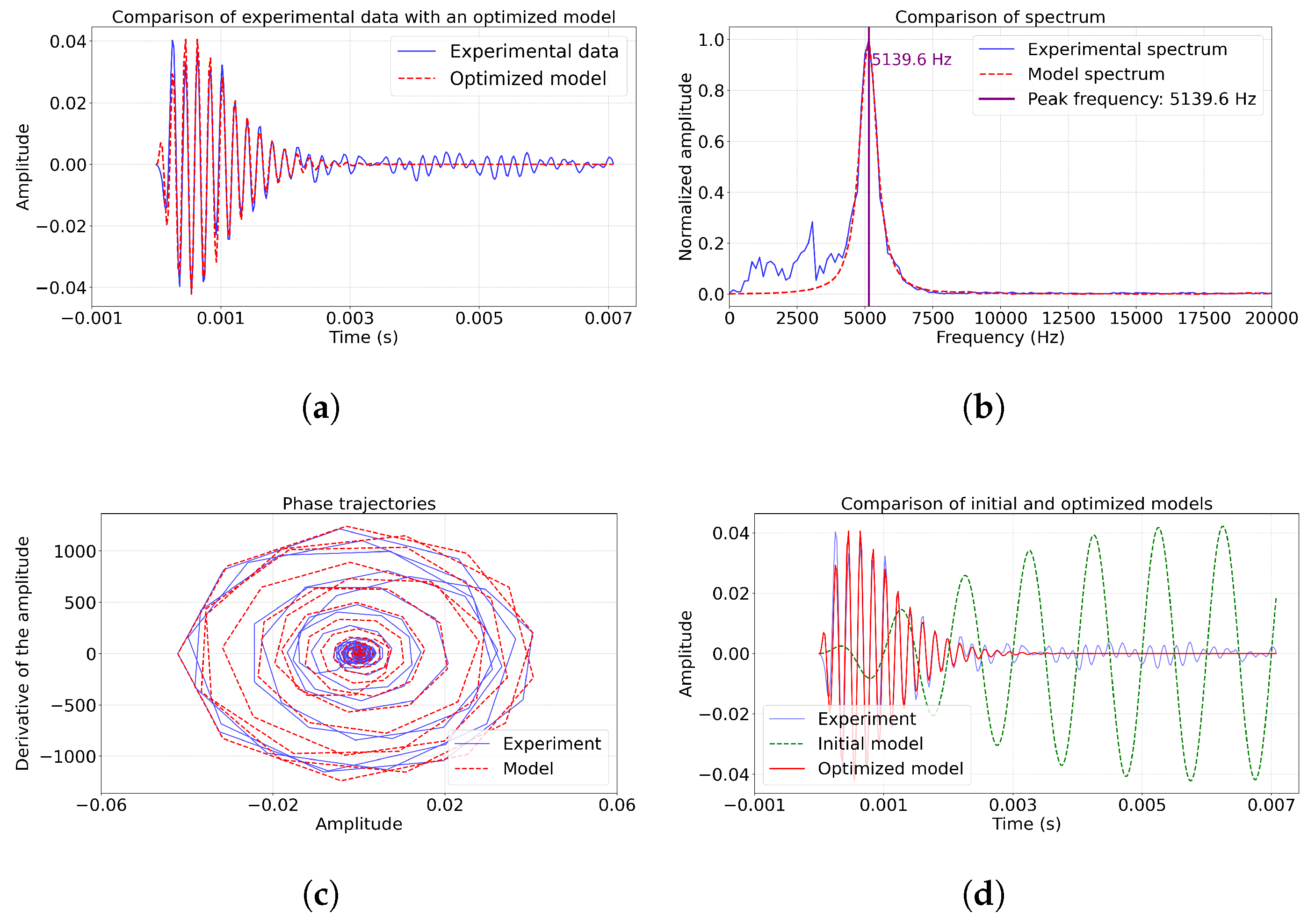
Figure 7.
Comparison of model impulse and experimental June 26, 2017 at 01:00:09 s.; (a) comparison of pulse amplitudes; (b) pulse spectra; (c) phase trajectories of pulses; (d) comparison with initial model.
Figure 7.
Comparison of model impulse and experimental June 26, 2017 at 01:00:09 s.; (a) comparison of pulse amplitudes; (b) pulse spectra; (c) phase trajectories of pulses; (d) comparison with initial model.
The graphs (Figure 6a, d) show that the optimized model () reproduces key pulse characteristics by amplitude, which corresponds to a reduction of the mean squared error by 97.65% compared to the initial model (). The coefficient of determination (example 2) indicates the explanation of 55.37% dispersion of data. The basic frequency 5145.4 Hz (Figure 6b) is well reproduced by the model. The phase trajectories (fig. 6c) have the same dynamics as in fig. 5c.
The Figure 7a,d shows that the model accurately reproduces both the build-up phase of the pulse and the pattern of fading. Of particular interest are the phase trajectories on Figure 7c, where the optimized model shows a substantially better match with experimental data compared to examples 1-2. The spectral analysis (Figure 7b) confirms the accurate reproduction of the basic frequency 5139.6 Hz and a significant improvement in the correspondence both in the low-frequency (up to 12%) and in the high-frequency ranges.
The model on Figure 8 achieved the best fit to the experimental data with a coefficient of determination of and a decrease in MSE of . The graphs show the coincidence of amplitude characteristics (Figure 8a) and phase trajectories (Figure 8c) (asymmetry of only 0.08), especially in the region of the main frequency of 3044.7 Hz (Figure 8b). At the same time, phase trajectories keep characteristic features of experimental data, which indicates the correctness of using the model (1). The results obtained, especially against previous examples (comparison with , and of MSE reduction) confirm the stable effectiveness of the two-step optimization method for different types of geoacoustic pulses.
The current model adequately describes the main characteristics of the pulse, but requires modification to accurately reproduce subtle dynamic features.

Table 1.
Optimized parameters of the mathematical model of high-frequency GAE using the differential evolution method (1 stage).
Table 1.
Optimized parameters of the mathematical model of high-frequency GAE using the differential evolution method (1 stage).
| Parameters | A | a | b | c | |
| Example 1 | 1.5612 | 1.5210 | 0.001104 | 19419.8 | 2.8133 |
| Example 2 | 1.2576 | 1.474 | 0.000295 | 32365.9 | 0.6822 |
| Example 3 | 1.4845 | 1.5061 | 0.5061 | 32640.2 | -0.4790 |
| Example 4 | 0.5551 | 0.9498 | 0.00115 | 19454.4 | -1.6688 |
Table 2.
Optimized parameters of the mathematical model of high-frequency GAE using the Nelder-Mead method (2 stage).
Table 2.
Optimized parameters of the mathematical model of high-frequency GAE using the Nelder-Mead method (2 stage).
| Parameters | A | a | b | c | |
| Example 1 | 1.6264 | 1.5206 | 0.001104 | 19419.8 | 2.8133 |
| Example 2 | 1.2981 | 1.4734 | 0.000295 | 32365.9 | 0.6823 |
| Example 3 | 1.5146 | 1.5059 | 0.000533 | 32640.2 | -0.4790 |
| Example 4 | 0.5614 | 0.9498 | 0.001159 | 19454.4 | -1.6688 |
To analyze the performance of the selected optimization methods, we calculated the following statistical parameters (Table 3): — Mean Squared Error, — MSE of the initial model, — coefficient of determination, – improvement of errors.
In all examples, a significant decrease in MSE was achieved (by 96.41-99.25 %) compared to the initial model. Best result (Example 4): MSE reduced to 1.35e-6 with an improvement of . High values of (0.5537-0.9755) confirm the adequacy of the model. The differential evolution method provided an initial gross reduction in MSE (seen by the difference of and MSE from Table 3). The method is especially effective in Examples 1-2 (complex cases with low ) (Table 3). The Nelder-Mead method gave the final fine tuning (achieving an MSE of about 1e-6). Maximum efficiency in examples 3-4 ().
5. Conclusions
The combined use of methods made it possible to achieve high quality approximation (MSE is reduced by 2 orders of magnitude), while the Nelder-Mead method provided accurate final adjustment of parameters. Double optimization significantly improved the model’s fit to experimental data. Optimizing the parameters of the model using a combination of the differential evolution method and the Nelder-Mead method significantly improved its accuracy. The optimized model closely follows the dynamics of geoacoustic emission, including the moments of pulse generation and their attenuation. Coincidence is observed not only in the main peaks, but also in the smaller amplitudes of the signals, which confirms the adequacy of the model.
It was found that the geoacoustic emission pulses that are most similar to the Berlage functions have a coefficient of determination of and an improvement of . The results obtained indicate that the proposed model correctly describes the process of generating acoustic pulses during deformation of geological environments. The results confirm the prospects of using the Berlage oscillator for the analysis of high-frequency GAE.
For further development of the work, it is planned to scale the experimental data and the considered optimization methods to the case of a chain of coupled Berlage oscillators with two or more interconnected dislocation sources of GAE. In general, the relationship between dislocation sources may be nonlinear, which can significantly complicate the study. Therefore, it will be necessary to use modern neural network methods [25].
Another continuation of the GAE study is related to its comparison with other studies in various geophysical fields, for example, such as the radon field [26] or the electromagnetic field [27,28], as well as a number of others. Such an integrated approach, in our opinion, should bring us closer to developing more effective methods for monitoring and diagnosing natural environments.
Author Contributions
Conceptualization, R.I. and D.F.; methodology, R.I.; software, D.F. and R.I.; validation, R.I., D.F.; formal analysis, R.I.; investigation, D.F., R.I.; resources, D.F., R.I.; writing—original draft preparation, D.F., R.I.; writing—review and editing, R.I.; visualization, D.F., R.I. All authors have read and agreed to the published version of the manuscript.
Funding
The work was carried out within the framework of the State Assignment of IKIR FEB RAS (reg. topic №124012300245-2)
Institutional Review Board Statement
Not applicable.
Informed Consent Statement
Not applicable.
Data Availability Statement
The data on earthquakes considered in the article are available at the Unified Information System of Seismological Data of the Kamchatka Branch of Geophysical Service Russian Academy of Science at http://sdis.emsd.ru/info/earthquakes/catalogue.php (accessed on 19 August 2025).
Conflicts of Interest
The authors declare no conflict of interest.
Abbreviations
| GAE | Geoacoustic Emission |
| IKIR FEB RAS | Institute of Cosmophysical Research and Radio Wave Propagation of the Far Eastern Branch of the Russian Academy of Sciences |
| MSE | Mean Squared Error |
References
- Marapulets, Y.; Solodchuk, A.; Lukovenkova, O.; Mishchenko, M.; Shcherbina, A. Sound Range AE as a Tool for Diagnostics of Large Technical and Natural Objects. Sensors 2023, 23, 1269. [CrossRef]
- Vassilyev, I.; Mendakulov, Z.; Imansakipova, B.; Aitkazinova, S.; Issabayev, K.; Imansakipova, N.; Madimarova, G. Acoustic emission spectrum for mine hazards identification and prevention. Sci. Rep. 2025 15, 6408. [CrossRef]
- Zhang, K.; Zhang, D.; Zhao, Y.; et al. "Experimental study on acoustic emission evolution characteristics and response mechanism of damaged rocks. Coal Geology & Exploration 2024, 52, 11.
- Song, J.; Leng, J.; Li, J.; Wei, H.; Li, S.; Wang, F. Application of Acoustic Emission Technique in Landslide Monitoring and Early Warning: A Review. Appl. Sci. 2025, 15, 1663. [CrossRef]
- Pulinets, S.; Herrera, V.M.V. Earthquake Precursors: The Physics, Identification, and Application. Geosciences 2024, 14, 209. [CrossRef]
- Fa, L.; Yang, H.; Fa, Y.; Meng, S.; Bai, J.; Zhang, Y.; Zhao, M. Progress in acoustic measurements and geoacoustic applications. AAPPS Bull. 2024, 34, 23. [CrossRef]
- Gapeev, M.I.; Solodchuk, A.A.; Parovik, R.I. Coupled oscillators as a model of high-frequency geoacoustic emission. Vestn. KRAUNC. Fiz.-Mat. Nauki 2022, 40, 88–100. [CrossRef]
- Sergienko, D.F.; Parovik, R.I. On a system of coupled linear oscillators with fractional friction and nonconstant coefficients for describing geoacoustic emission. Vestn. KRAUNC. Fiz.-Mat. Nauki 2024, 49, 36–49. [CrossRef]
- Price, K.; Storn, R.; Lampinen, J. Differential Evolution: A Practical Approach to Global Optimization; Springer: Berlin, Germany, 2005.
- Nelder, J.A.; Mead, R. A simplex method for function minimization. Comput. J. 1965, 7, 308–313. [CrossRef]
- Larionov, I.A.; Marapulets, Yu.V.; Mishchenko, M.A. Simultaneous lithospheric-atmospheric signals of acoustic emission at "Karymshina" site in Kamchatka. EPJ Web Conf. 2021, 254, 02013. [CrossRef]
- Mishchenko, M.A. et al. Joint analysis of low-frequency geoacoustic and deformation signals. EPJ Web Conf. 2018, 262, 02009.
- Lukovenkova, O.O.; Marapulets, Yu.V.; Solodchuk, A.A. Adaptive Approach to Time-Frequency Analysis of AE Signals of Rocks. Sensors 2022, 22, 9798. [CrossRef]
- Larionov, I.A. et al. Prototype of an automated hardware-software complex for operational monitoring, identification, and analysis of geophysical signals. Vestn. KRAUNC. Fiz.-Mat. Nauki 2018, 24, 213–225.
- Larionov, I.A. et al. Studies of acoustic emission of near-surface sedimentary rocks in Kamchatka. Geosist. Perekhodnykh Zon 2017, 1, 57–63.
- Lukovenkova, O.O.; Solodchuk, A.A. Analysis of geoacoustic emission and electromagnetic radiation signals accompanying earthquake with magnitude Mw=7.5. E3S Web Conf. 2020, 196, 03001.
- Marapulets, Yu.V.; Shcherbina, A.O.; Solodchuk, A.A.; Mishchenko, M.A. Localization of Rock Acoustic Emission Sources Based on a Spaced Sensors System Consisting of Two Combined Receivers and a Hydrophone. Sensors 2025, 25, 1197. [CrossRef]
- Marapulets, Yu.V.; Lukovenkova, O.O. Time-frequency analysis of geoacoustic data using adaptive matching pursuit. Acoust. Phys. 2021, 67, 312–319. [CrossRef]
- Artemev, A.E. Physical Foundations of Seismic Exploration; Nauka: Saratov, Russia, 2012; p. 56.
- Senkevich, Yu.I.; Lukovenkova, O.O.; Solodchuk, A.A. Methodology for forming a Register of geophysical signals using geoacoustic emission signals as an example. Geosist. Perekhodnykh Zon 2018, 2, 409–418.
- Mingazova, D.F.; Parovik, R.I. Some aspects of qualitative analysis of the high-frequency geoacoustic emission model. Vestn. KRAUNC. Fiz.-Mat. Nauki 2023, 42, 191–206. [CrossRef]
- Storn, R.; Price, K. Differential Evolution – A Simple and Efficient Heuristic for Global Optimization over Continuous Spaces. J. Glob. Optim. 1997, 11, 341–359. [CrossRef]
- Mohamad Faiz, A.; Nor Ashidi, M.I. et al. Differential evolution: A recent review based on state-of-the-art works. Alexandria Eng. J. 2022, 61, 3831–3872.
- Tristanov, A.; Lukovenkova, O.; Marapulets, Yu.; Kim, A. Improvement of methods for sparse model identification of pulsed geophysical signals. In Proc. SPA-2019; IEEE: New York, NY, USA, 2019; pp. 256–260.
- Jiang, Z.; Zhu, Z.; Lacidogna, G.; Friedrich, L.F.; Iturrioz, I. Earthquake Precursors Based on Rock Acoustic Emission and Deep Learning. Sci 2025, 7, 103. [CrossRef]
- Tverdyi, D.; Makarov, E.; Parovik, R. Estimation of Radon Flux Density Changes in Temporal Vicinity of the Shipunskoe Earthquake with Mw = 7.0, 17 August 2024 with the Use of the Hereditary Mathematical Model. Geosciences 2025, 15, 30. [CrossRef]
- Lin, M.; Peng, X.; Chen, Y.; Liao, Q.; Lu, X.; Liu, X. Acoustic Emission and Infrared Radiation Energy Evolution in the Failure of Phosphate Rock: Characteristics and Damage Modeling. Appl. Sci. 2025, 15, 9001. [CrossRef]
- Venegas-Aravena, P.; Cordaro, E.G. Analytical Relation between b-Value and Electromagnetic Signals in Pre-Macroscopic Failure of Rocks: Insights into the Microdynamics’ Physics Prior to Earthquakes. Geosciences 2023, 13, 169. [CrossRef]
Figure 1.
General scheme for recording GAE.
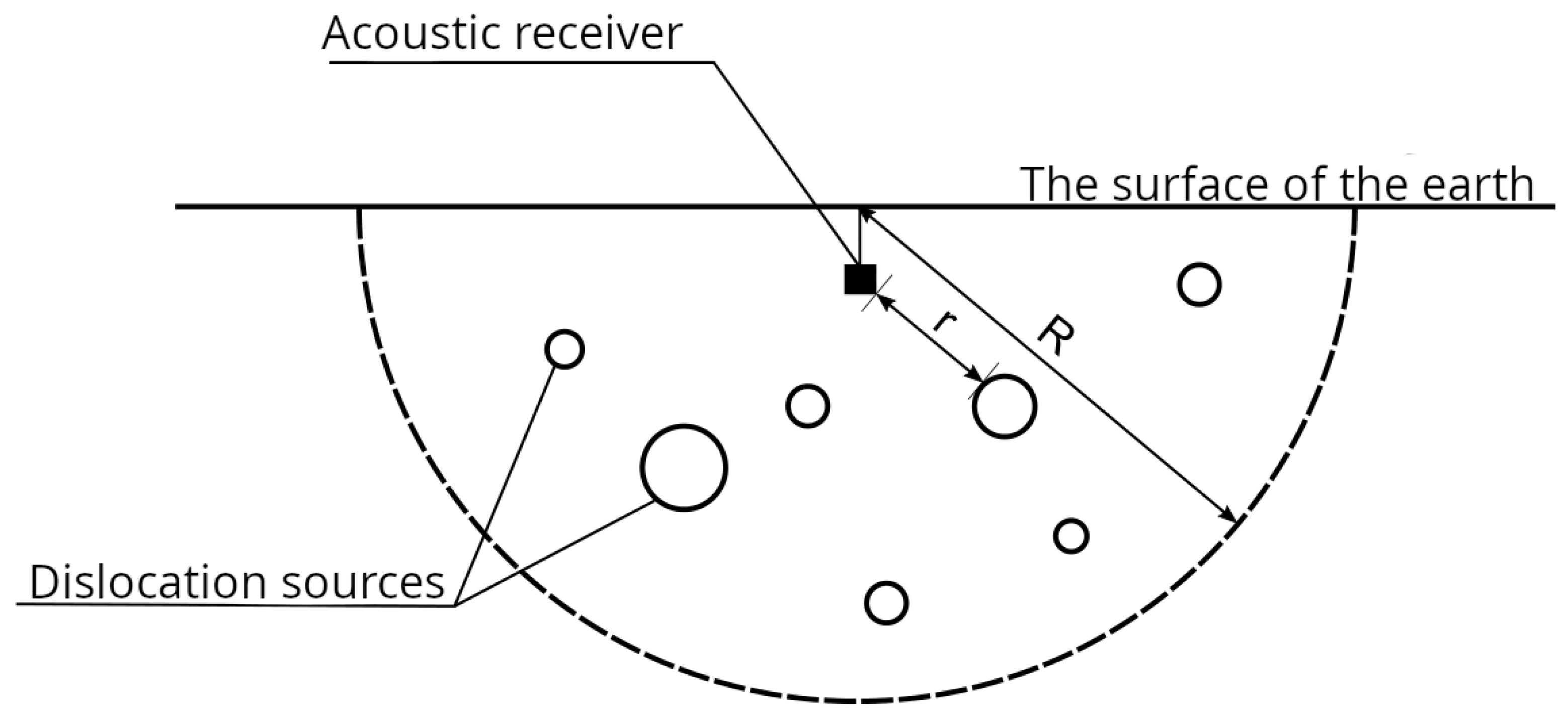
Figure 2.
GAE sensors: a) hydrophone Zetlab BC313, b) system of directed hydrophones, c) combined receiver.
Figure 2.
GAE sensors: a) hydrophone Zetlab BC313, b) system of directed hydrophones, c) combined receiver.
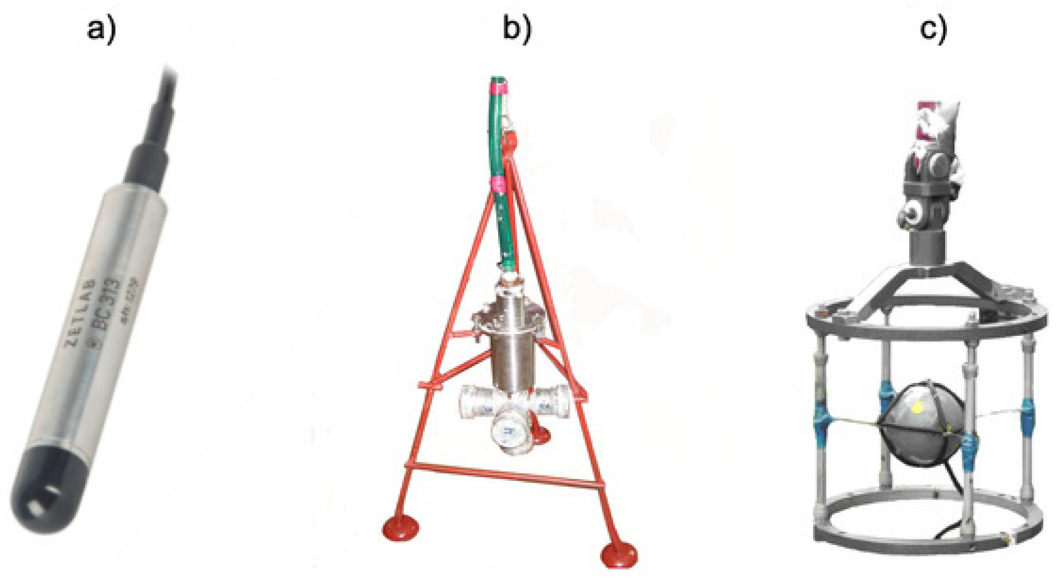
Figure 3.
Distribution of geoacoustic emission pulses before the earthquake 27 June 2017 02:23 UTC for 72 hours.
Figure 3.
Distribution of geoacoustic emission pulses before the earthquake 27 June 2017 02:23 UTC for 72 hours.
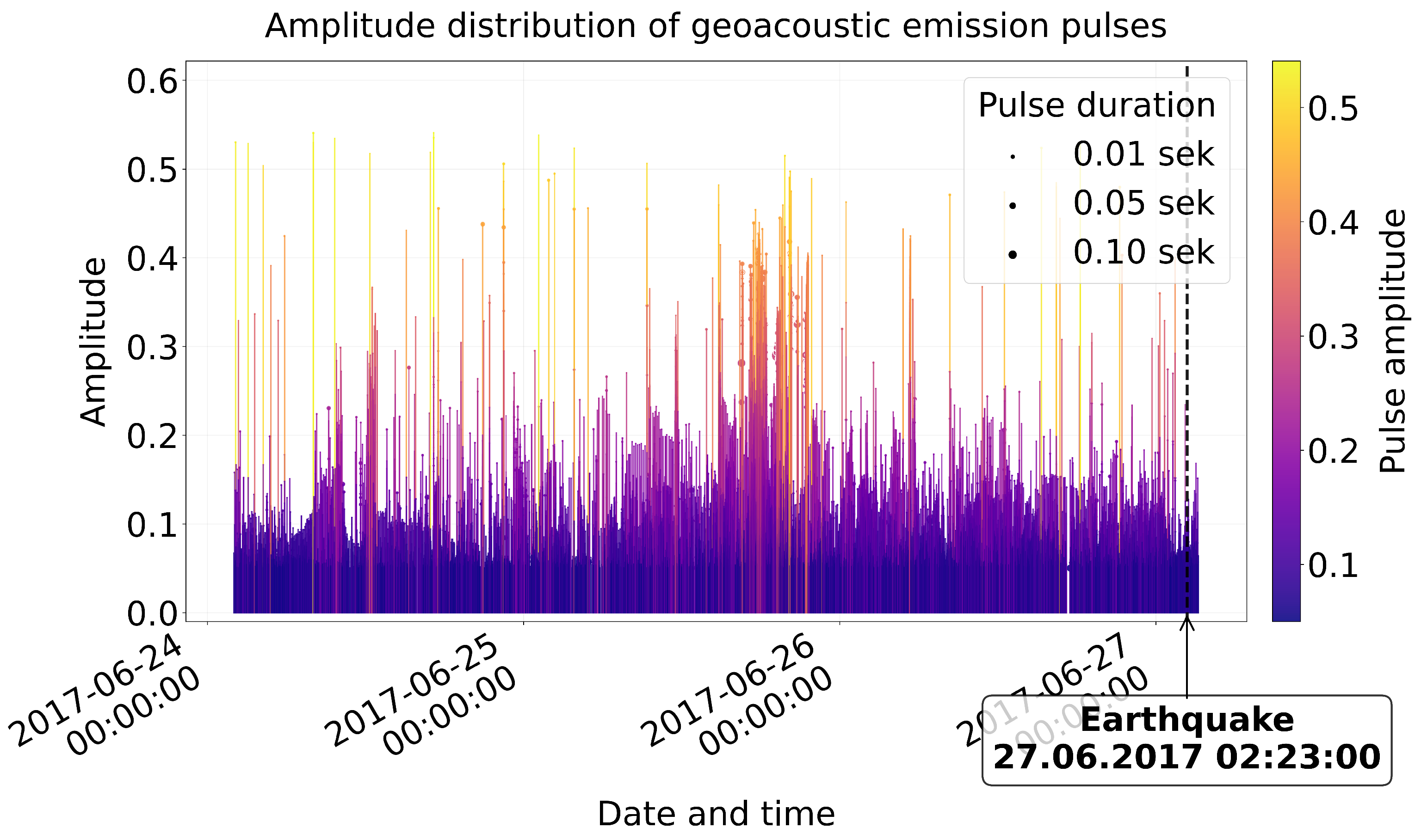
Figure 4.
Amplitude distribution of geoacoustic emission pulses before the earthquake on 27 June 2017 02:23 UTC for 50 hours: (a) general type of pulses, (b-d) detail of individual pulses.
Figure 4.
Amplitude distribution of geoacoustic emission pulses before the earthquake on 27 June 2017 02:23 UTC for 50 hours: (a) general type of pulses, (b-d) detail of individual pulses.
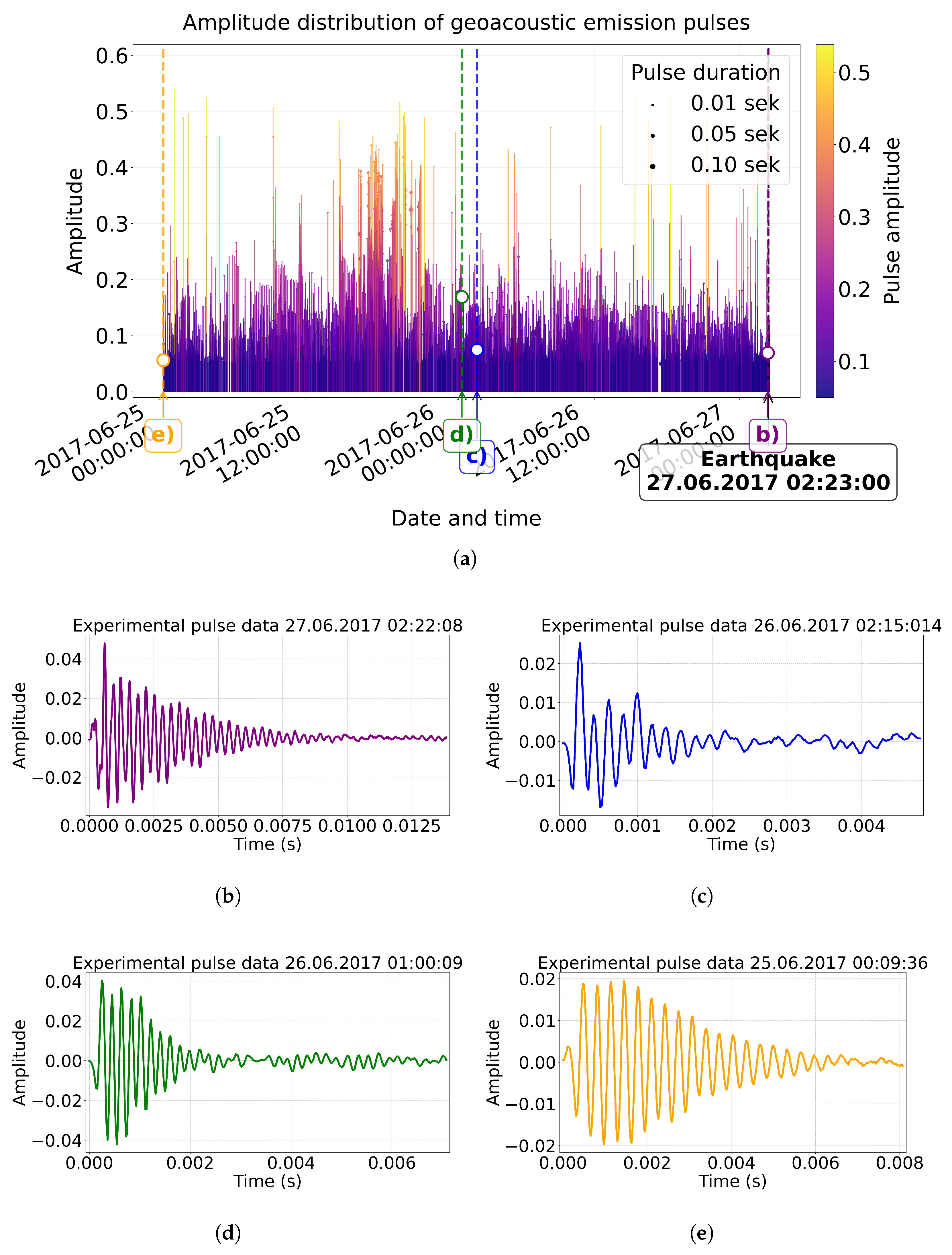
Figure 5.
Comparison of model impulse and experimental June 27, 2017 02:22:08 s.; (a) comparison of pulse amplitudes; (b) pulse spectra; (c) phase trajectories of pulses; (d) comparison with initial model.
Figure 5.
Comparison of model impulse and experimental June 27, 2017 02:22:08 s.; (a) comparison of pulse amplitudes; (b) pulse spectra; (c) phase trajectories of pulses; (d) comparison with initial model.

Figure 8.
Comparison of model impulse and experimental June 25, 2017 at 00:09:36 s.; (a) comparison of pulse amplitudes; (b) pulse spectra; (c) phase trajectories of pulses; (d) comparison with initial model.
Figure 8.
Comparison of model impulse and experimental June 25, 2017 at 00:09:36 s.; (a) comparison of pulse amplitudes; (b) pulse spectra; (c) phase trajectories of pulses; (d) comparison with initial model.
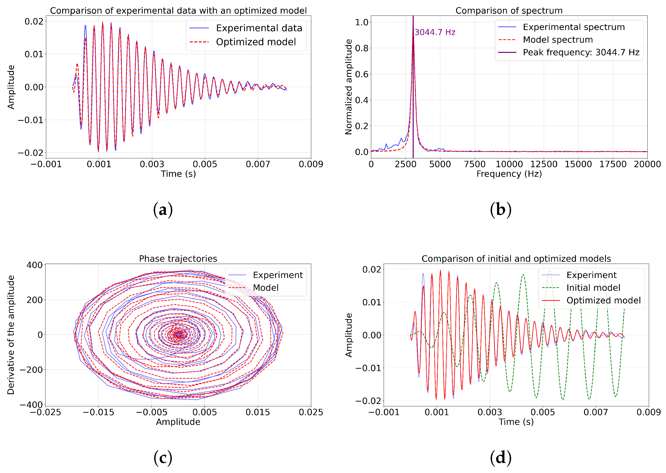
Table 3.
Statistical estimates of optimization parameters of the high-frequency GAE model.
| Example | MSE | |||
| 1 | 0.6623 | 96.41% | ||
| 2 | 0.5537 | 97.65% | ||
| 3 | 0.8947 | 99.12% | ||
| 4 | 0.9755 | 99.25% |
Disclaimer/Publisher’s Note: The statements, opinions and data contained in all publications are solely those of the individual author(s) and contributor(s) and not of MDPI and/or the editor(s). MDPI and/or the editor(s) disclaim responsibility for any injury to people or property resulting from any ideas, methods, instructions or products referred to in the content. |
© 2025 by the authors. Licensee MDPI, Basel, Switzerland. This article is an open access article distributed under the terms and conditions of the Creative Commons Attribution (CC BY) license (http://creativecommons.org/licenses/by/4.0/).
Copyright: This open access article is published under a Creative Commons CC BY 4.0 license, which permit the free download, distribution, and reuse, provided that the author and preprint are cited in any reuse.


