Submitted:
20 August 2025
Posted:
22 August 2025
You are already at the latest version
Abstract
The viral disease COVID-19, declared a pandemic by the World Health Organization (WHO), primarily affects the respiratory system and can be fatal. Although the Reverse Transcriptase Polymerase Chain Reaction (RT-PCR) test remains the gold standard for COVID-19 diagnosis, its time-intensive nature limits its effectiveness in urgent situations. To address this, we propose an ensemble of five state-of-the-art transfer learning (TL) models designed to mitigate biases and enhance the classification of COVID-19 from chest radiographs. A weighted optimization strategy combines the models, giving more weight to those with superior performance, ensuring more accurate and robust predictions. Evaluated on a publicly available dataset, the SqueezeNet model achieved the highest accuracy of 94.01% for three-class classification (Normal, COVID-19, Lung Opacity), while the ensemble approach achieved 92.57% accuracy and an F1-score of 92.36%, demonstrating resilience to transfer learning biases. This framework offers reliable diagnostic support, streamlining radiology workflows and enhancing decision-making in high-demand clinical environments. Additionally, it serves as a valuable tool for advancing medical artificial intelligence expertise among graduates.
Keywords:
1. Introduction
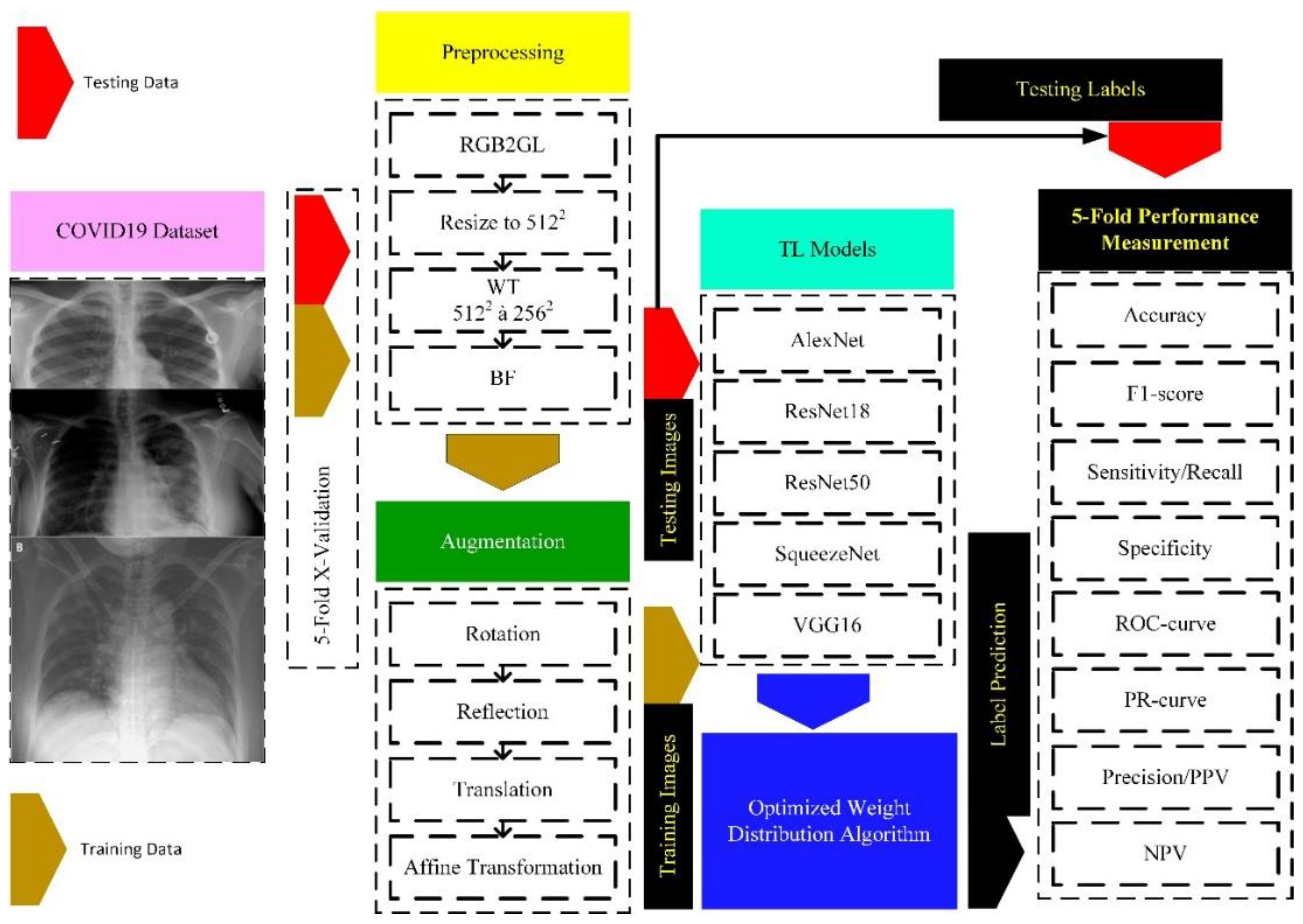
- The article proposes the design and implementation of DL-based TL methods tailored for the robust detection of C19 from chest radiographs and CT scans using a weight-optimized distribution algorithm. The metrics, from each of the large DL architectures, are normalized by dividing each metric by the sum of the corresponding metrics from all models. This normalization ensures that each metric’s influence is proportional to the individual performance of each of the five models.
- It uses an extensive dataset with variations to make it more challenging. The good classification ability of Class A could negatively impact the performance of Classes B and C due to feature dominance. We have used the first three classes (C19, LO, N) to make the task challenging. The last class achieves outstanding results, specifically, due to its discriminative characteristics, which can otherwise lead to negatively biased performance.
- It explicitly tackles the variation in imaging features across five different DL algorithms, improving differentiation between C19 manifestations in young versus elderly patients.
- The study addresses limitations of the traditional RT-PCR test, such as lower Sn (~59%), longer turnaround times, and the need for specialized laboratories, by offering a non-invasive, cost-effective AI-based diagnostic tool suitable for resource-limited settings.
- Support for Clinical Decision-making and Medical Education: Beyond assisting radiologists with a reliable second opinion in image interpretation, the proposed framework presents a valuable educational tool for medical graduates.
1.1. Related Work
2. Materials and Methods
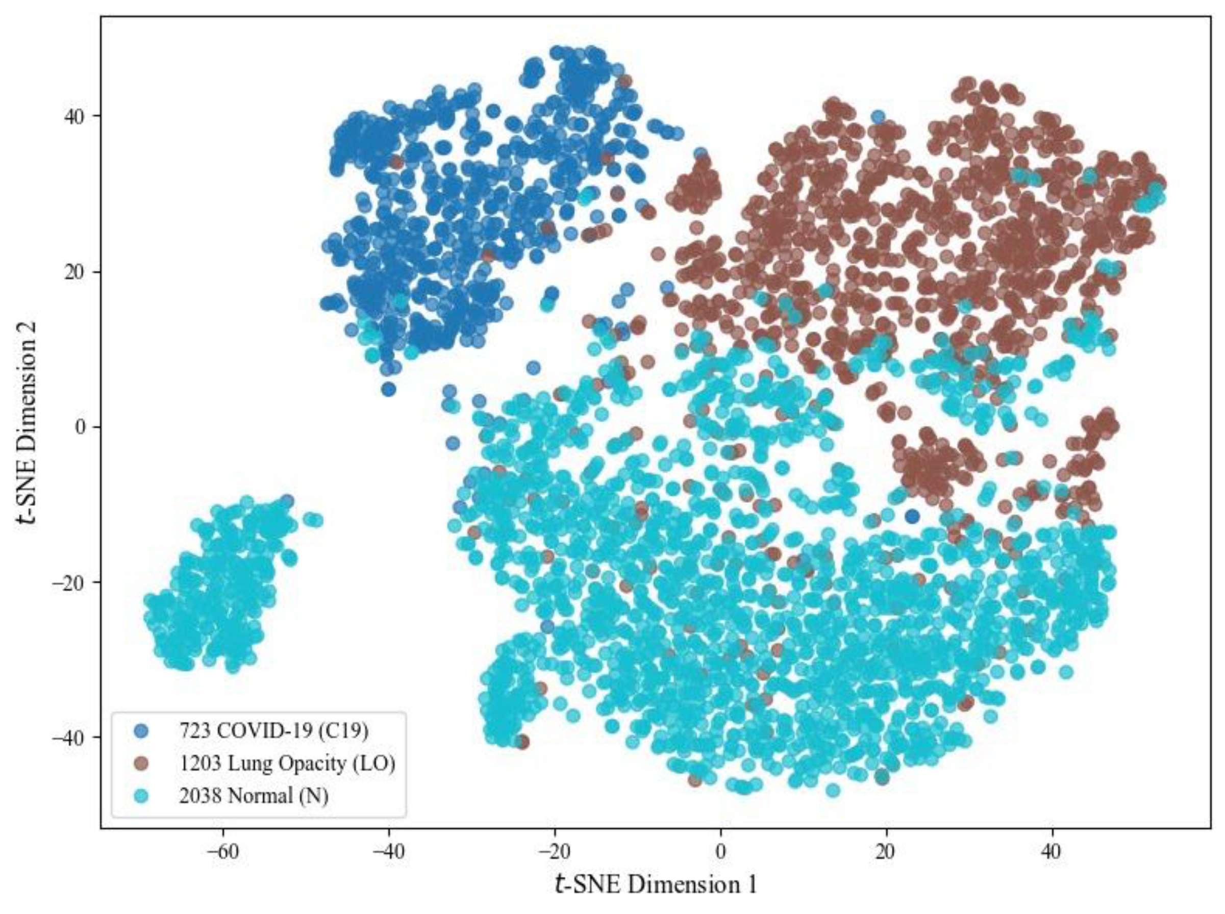
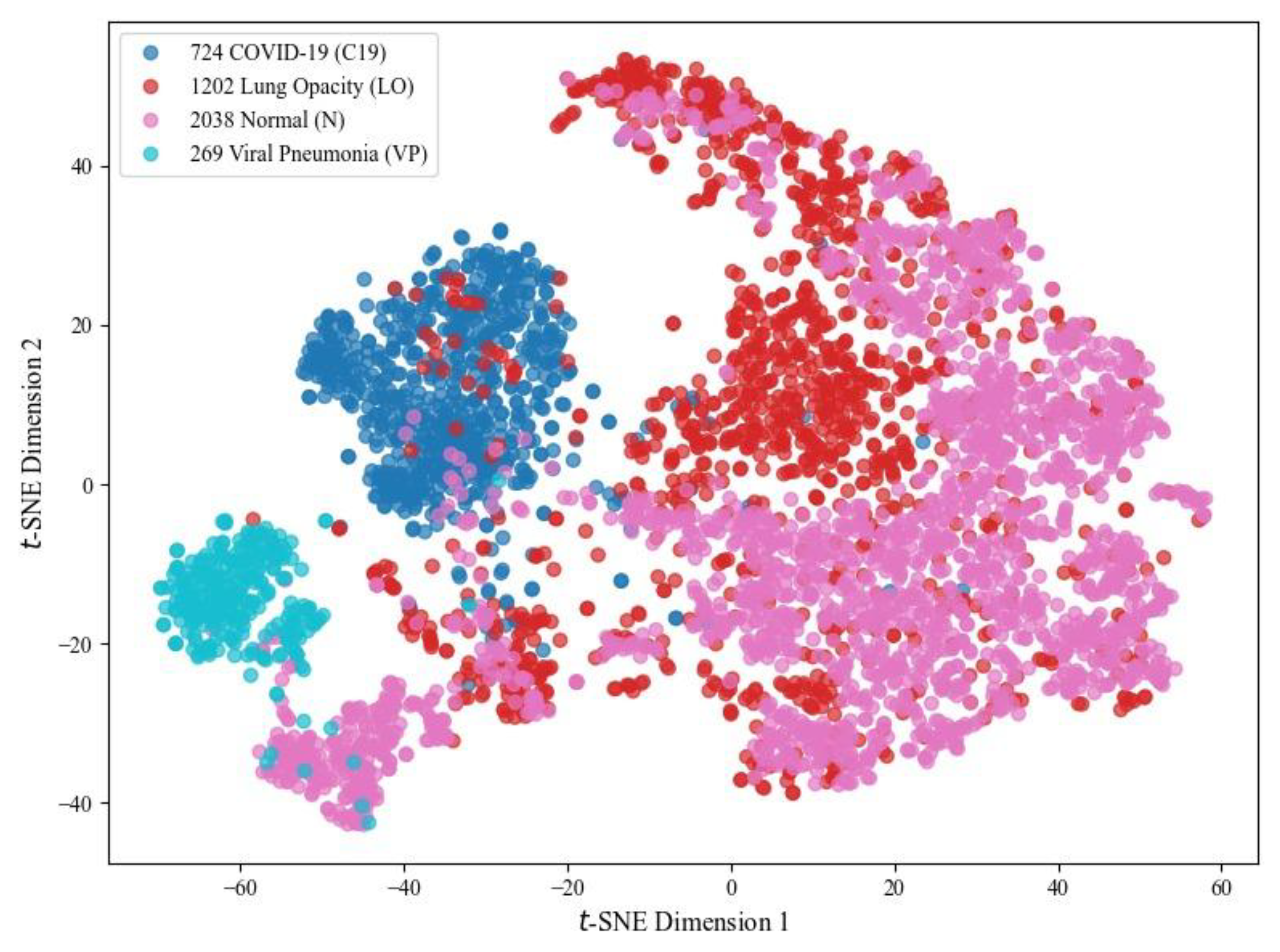
2.1. Dataset
2.2. Preprocessing
2.2.1. RGB to Grey-Scale Conversion
2.2.2. Resizing the Scans
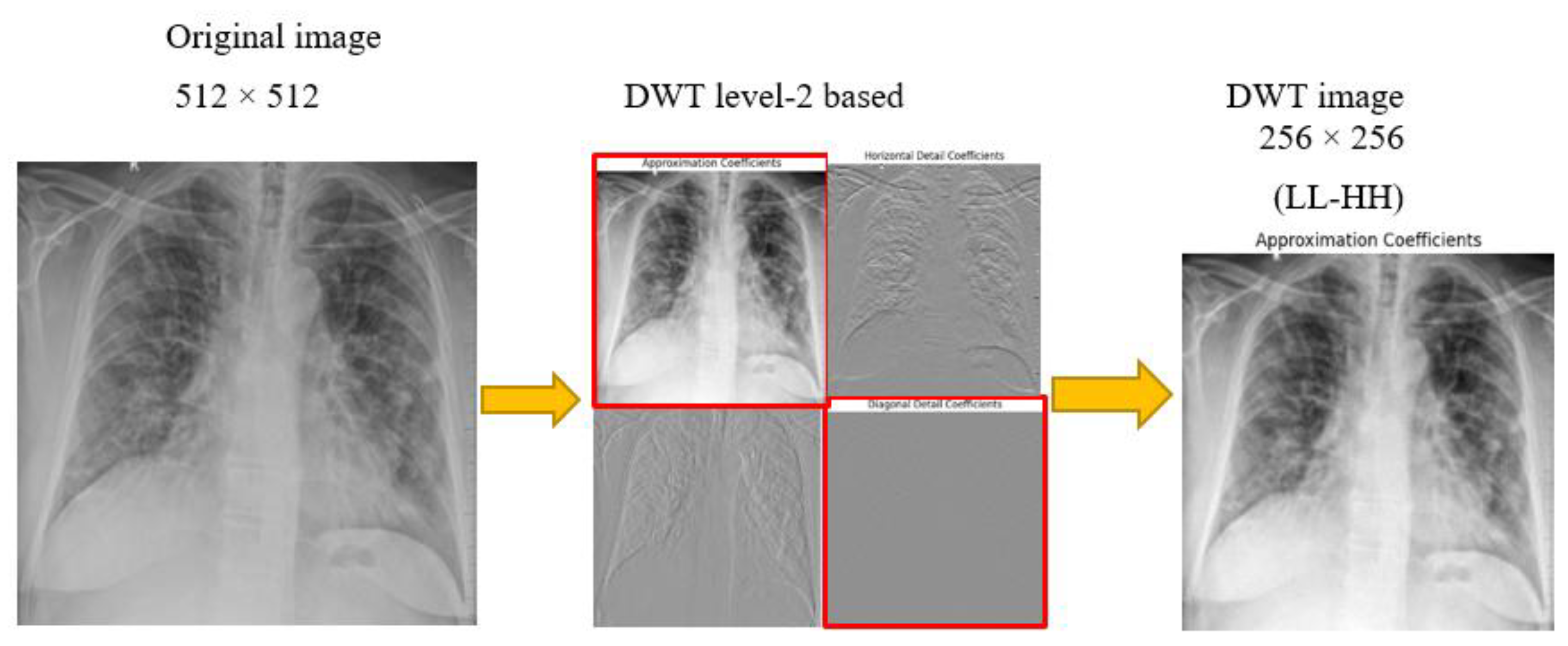
2.2.3. Discrete Wavelet Transform
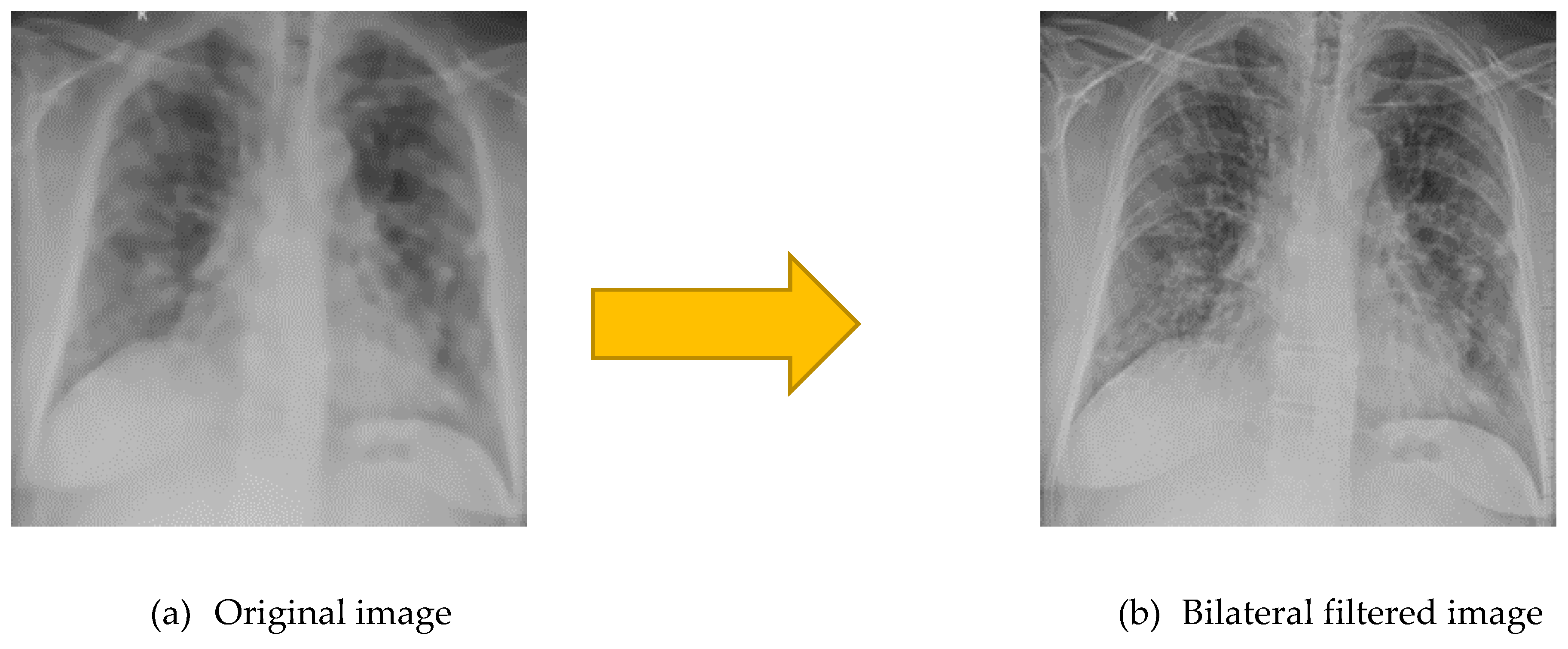
2.2.4. Bilateral Filtering
2.2.5. Augmentation
2.3. DL Overview
2.3.1. Minibatch Size
2.3.2. Dropout
2.3.3. Activation Functions
2.3.4. Softmax
2.3.5. Loss Function
2.3.6. Convolution Layers
2.3.7. MaxPooling
2.3.8. Fully Connected Layers
2.3.9. Batch Normalization
2.3.10. Adam Optimizer
2.4. TL-based DL Models
2.4.1. AlexNet
2.4.2. ResNet18
2.4.3. ResNet50
2.4.4. SqueezeNet
2.4.5. VGG16
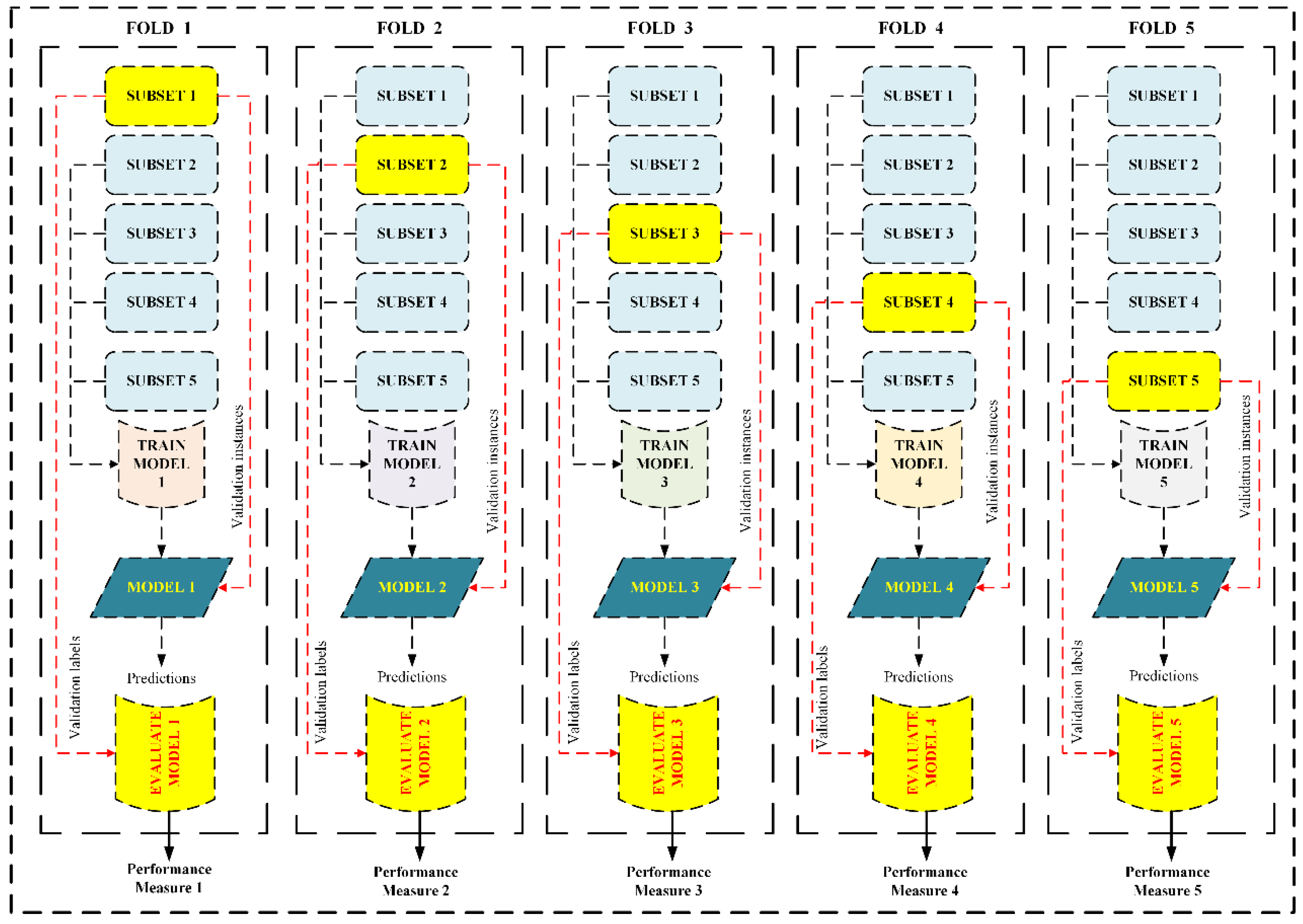
2.5. 5-Fold CV
2.6. Performance Measures
2.6.1. Accuracy
2.6.2. Specificity
2.6.3. Sn (Recall)
2.6.4. Precision (Positive Predicted Value)
2.6.5. Negative Predicted Value
2.6.6. F1 – Score
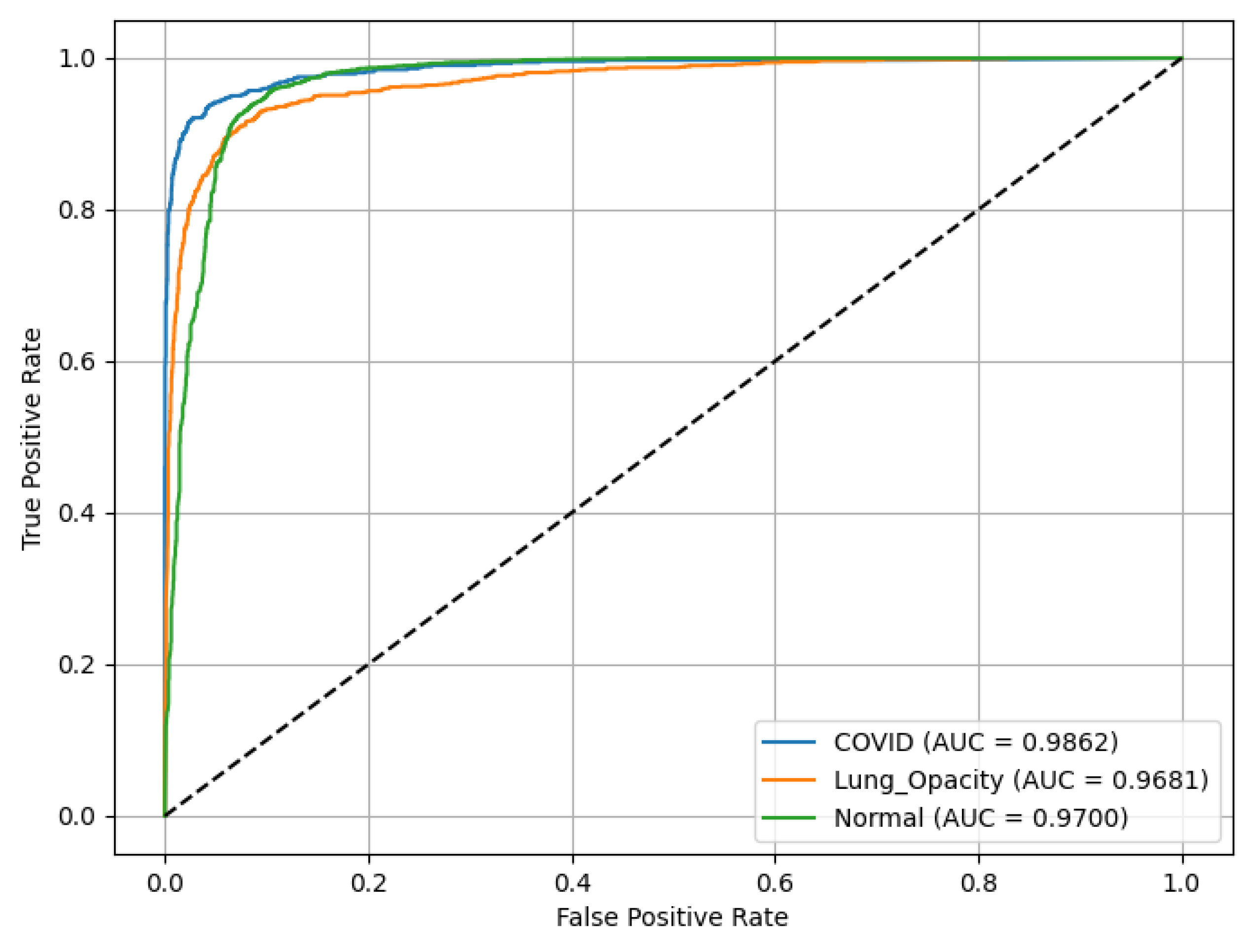
2.6.7. Area Under the Receiver Operating Characteristic ROC(AUC) curve
2.6.8. Area Under the Precision Recall PR(AUC) curve
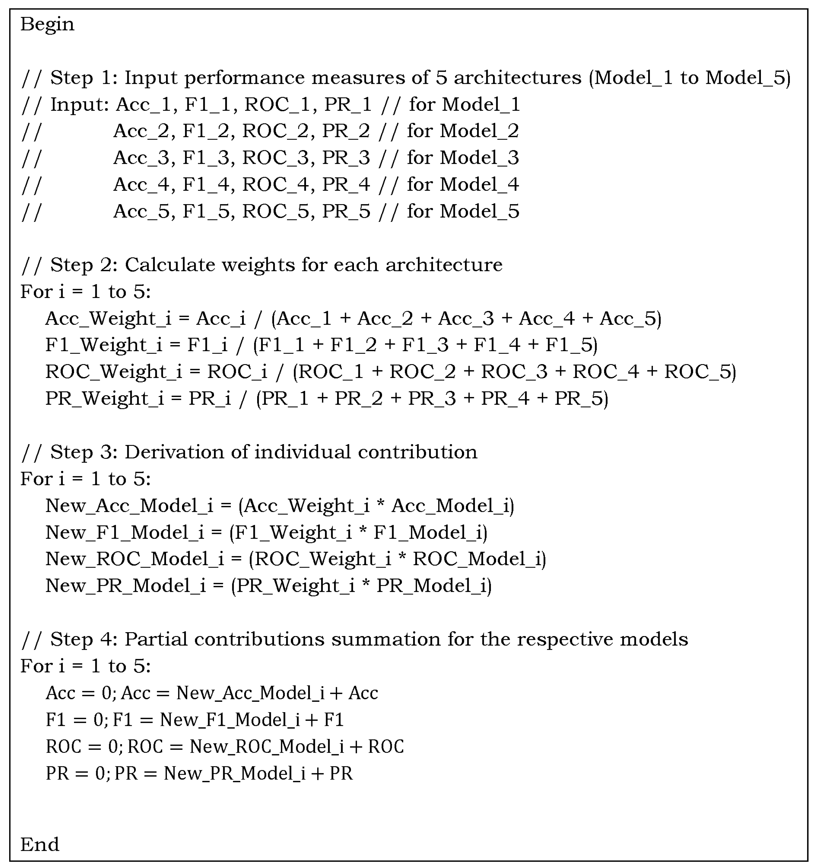
2.7. Optimized Weight Distribution Algorithm
3. Results and Discussion
3.1. AlexNet
3.2. ResNet18
3.3. ResNet50
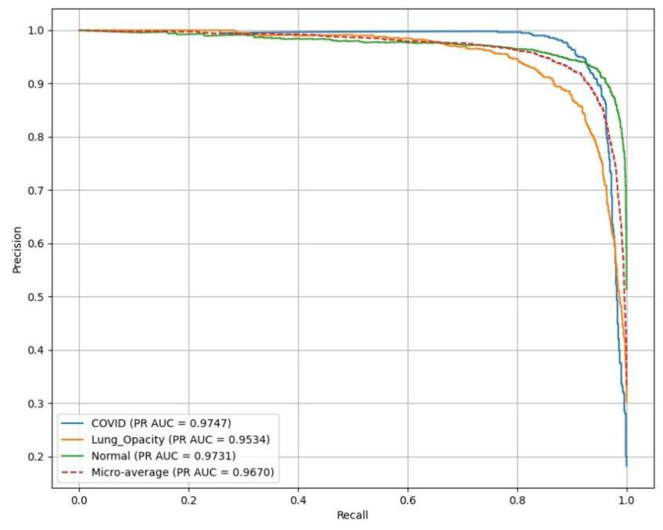
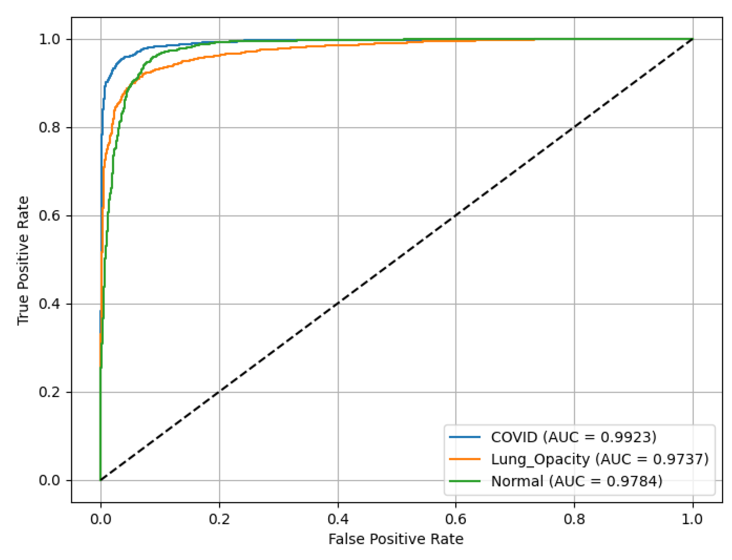
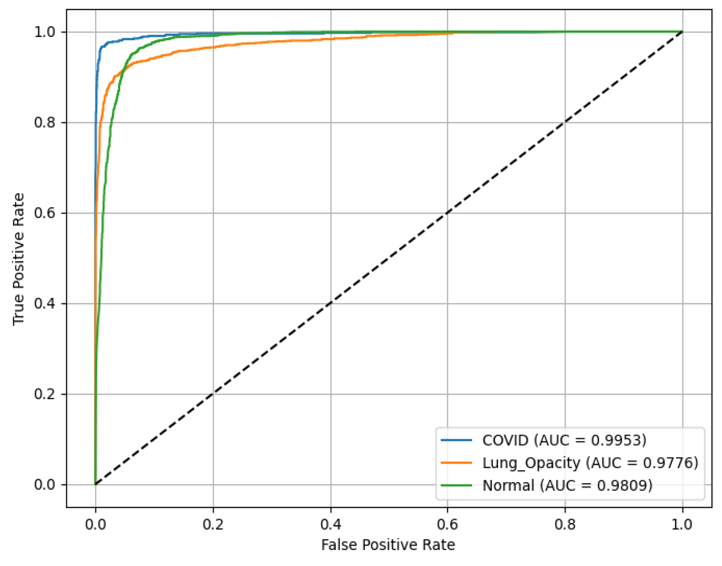
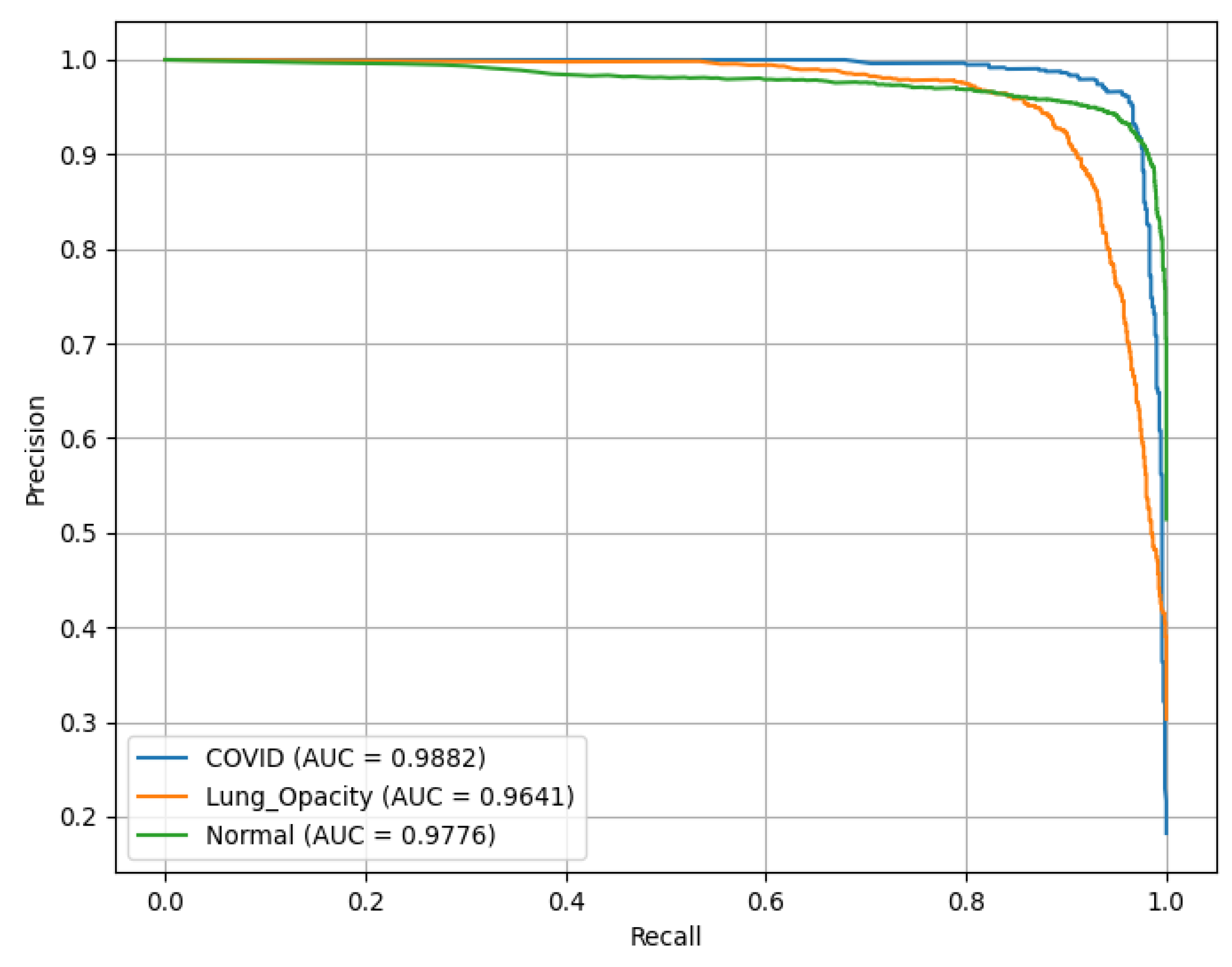
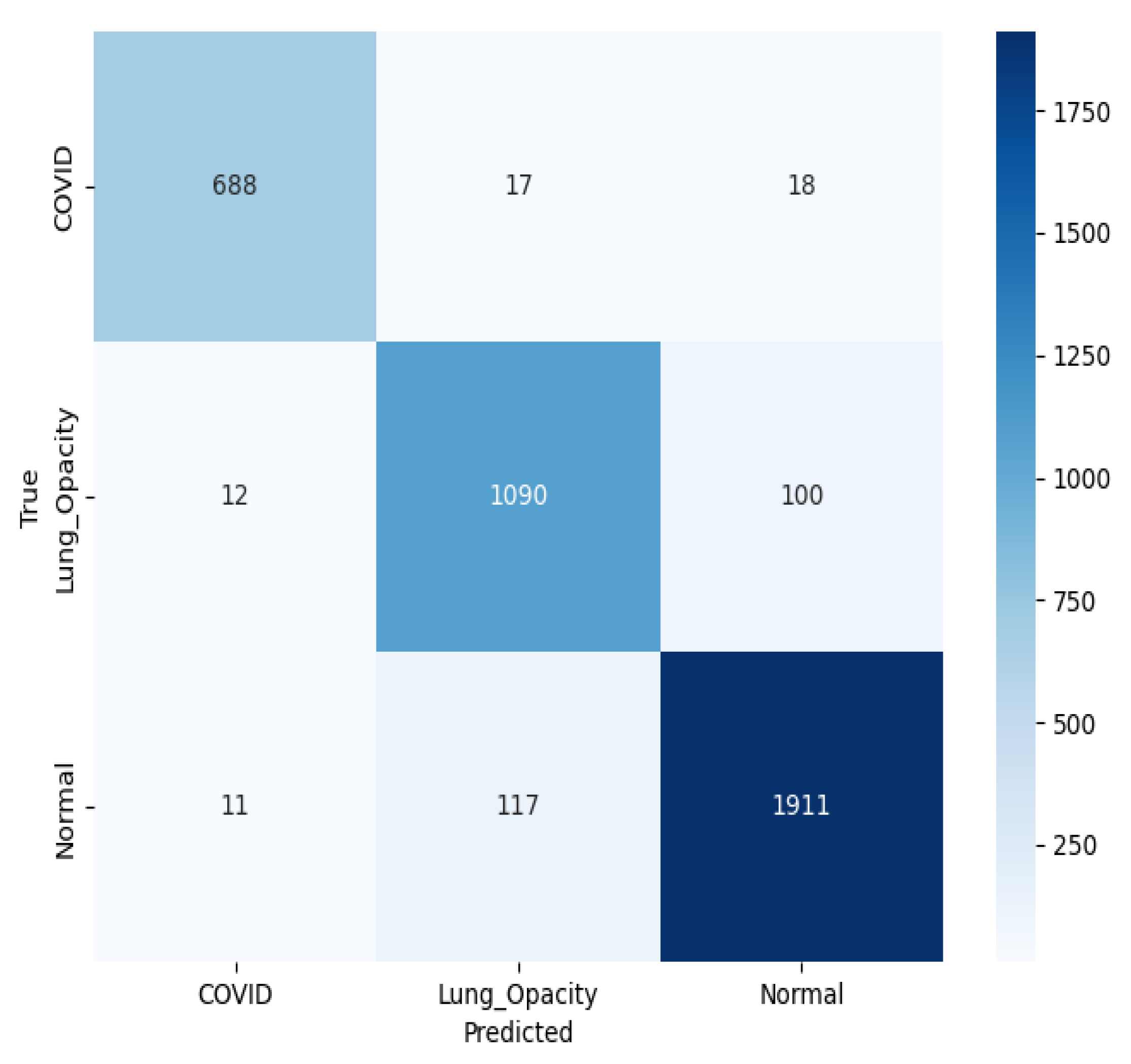
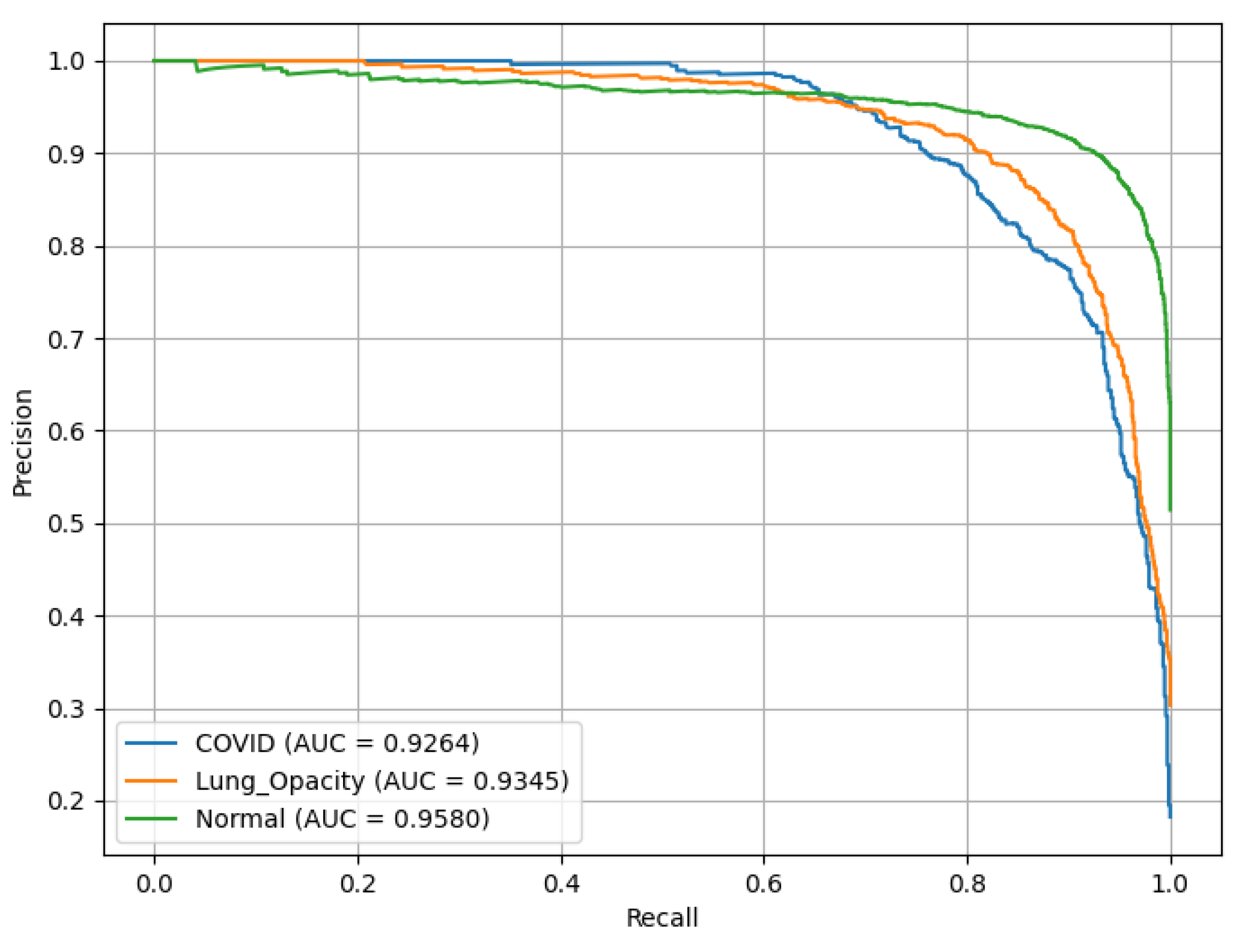
3.4. SqueezeNet
3.5. VGG16
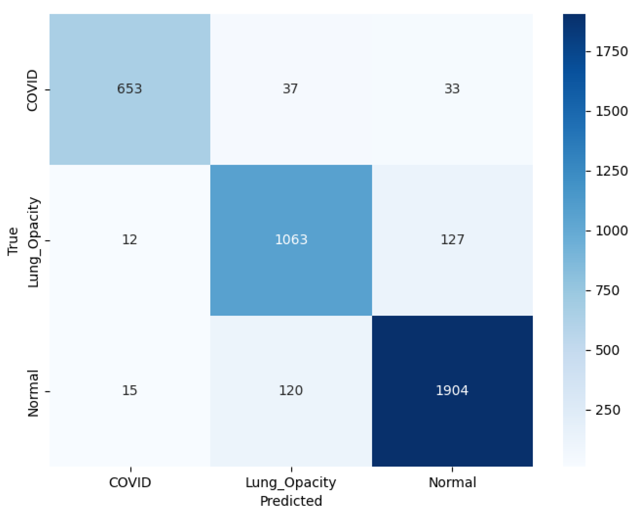
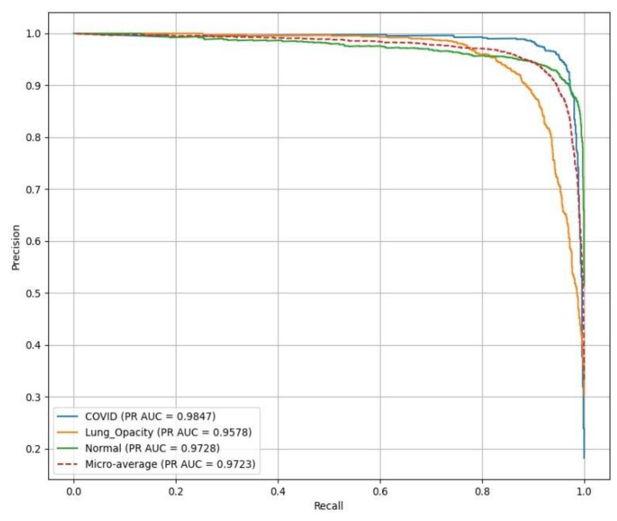
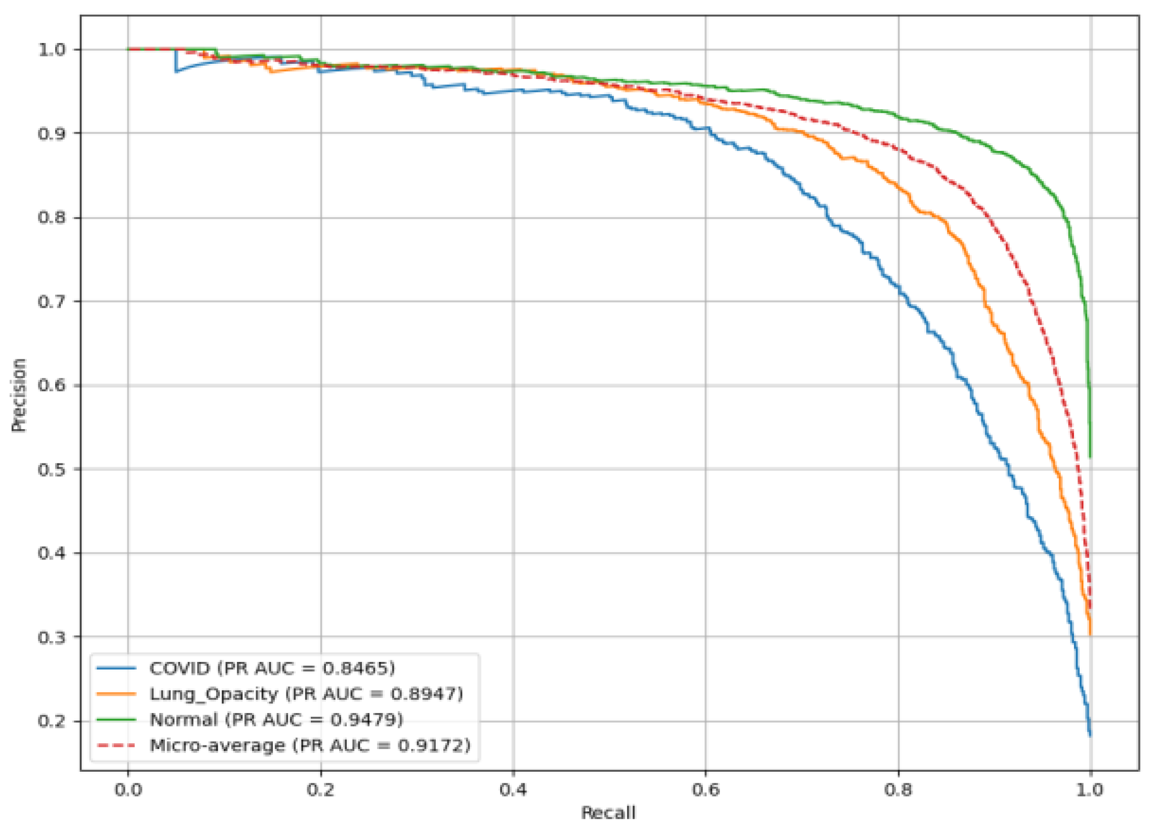
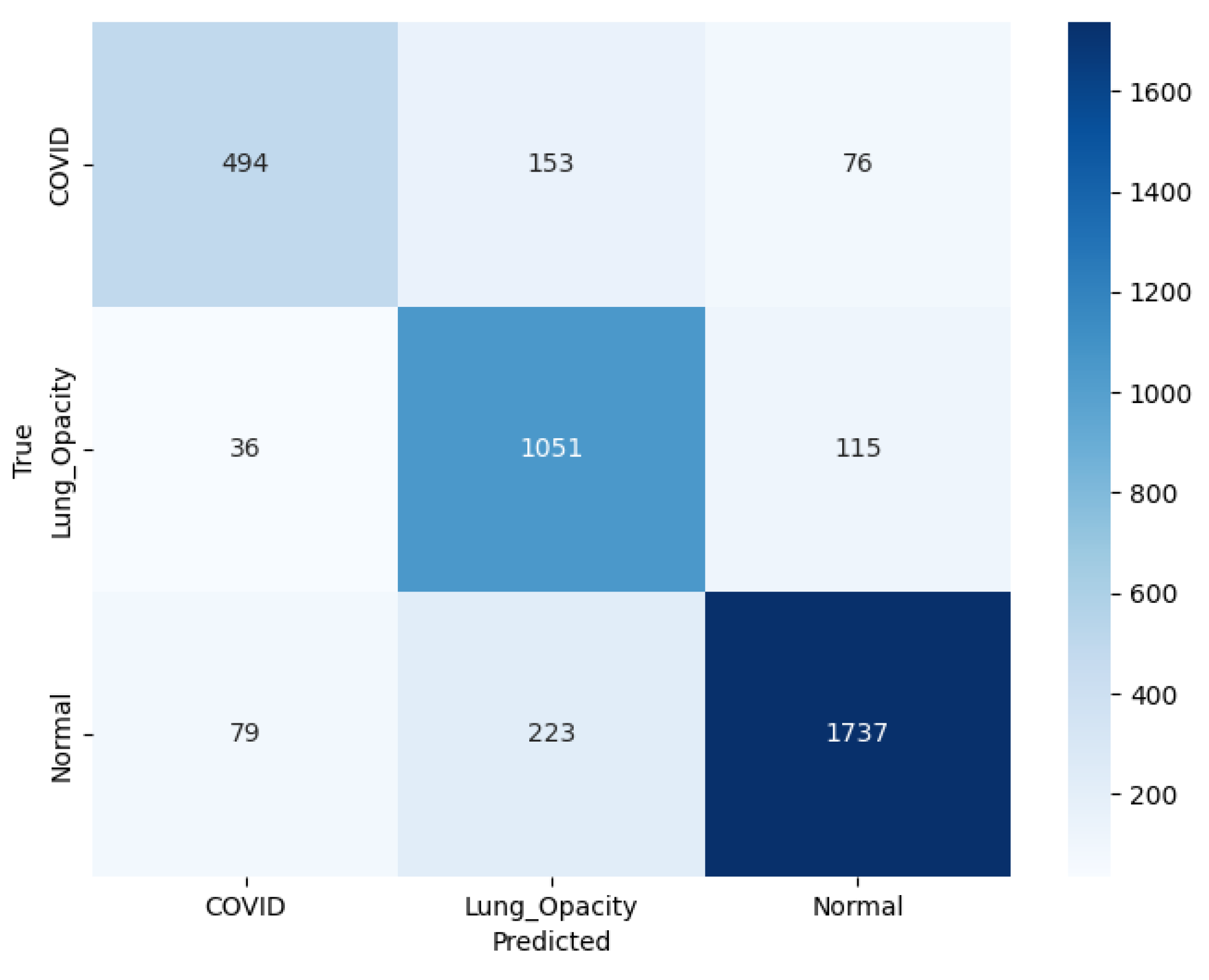
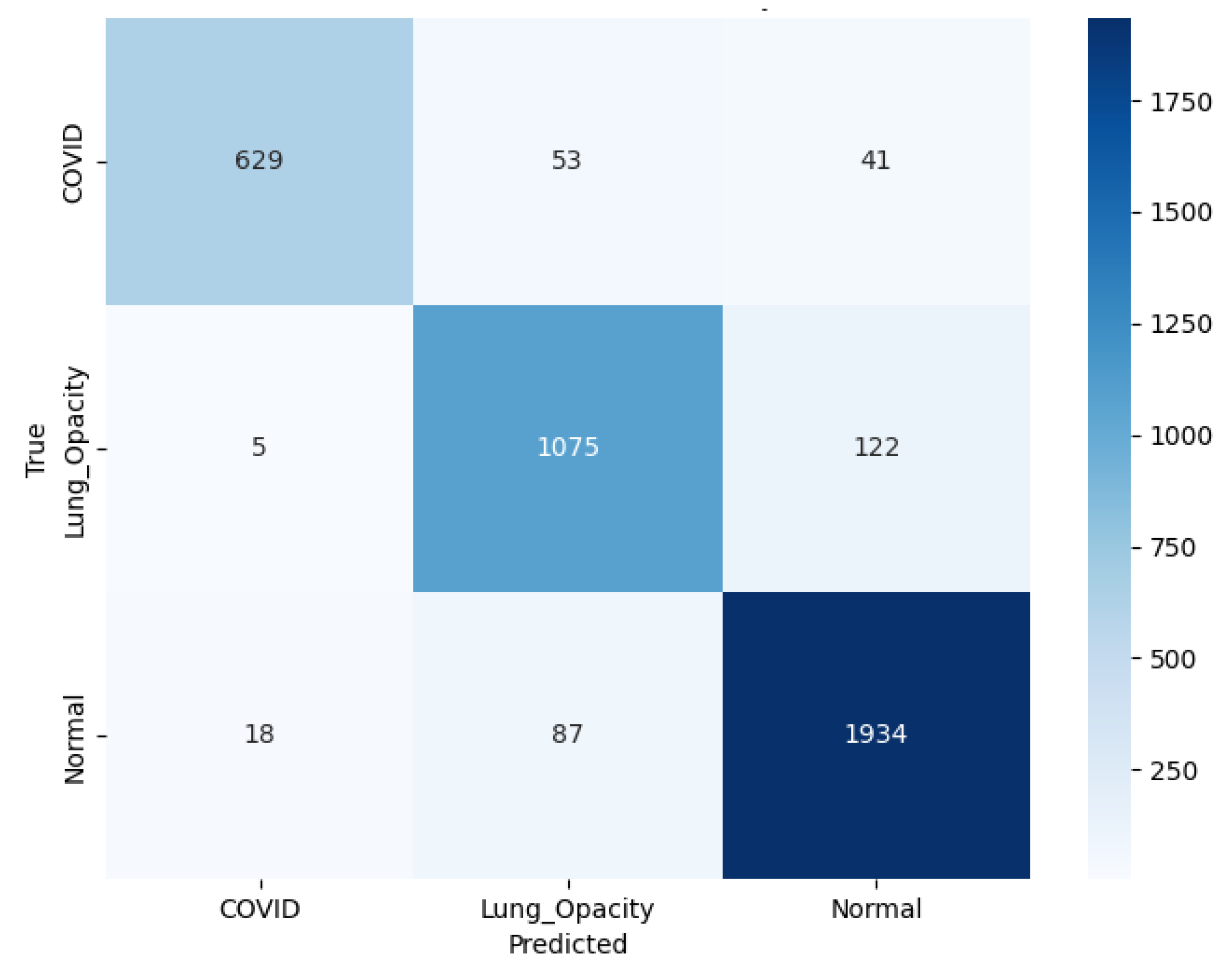
3.6. Ensemble Contribution Aggregation Results
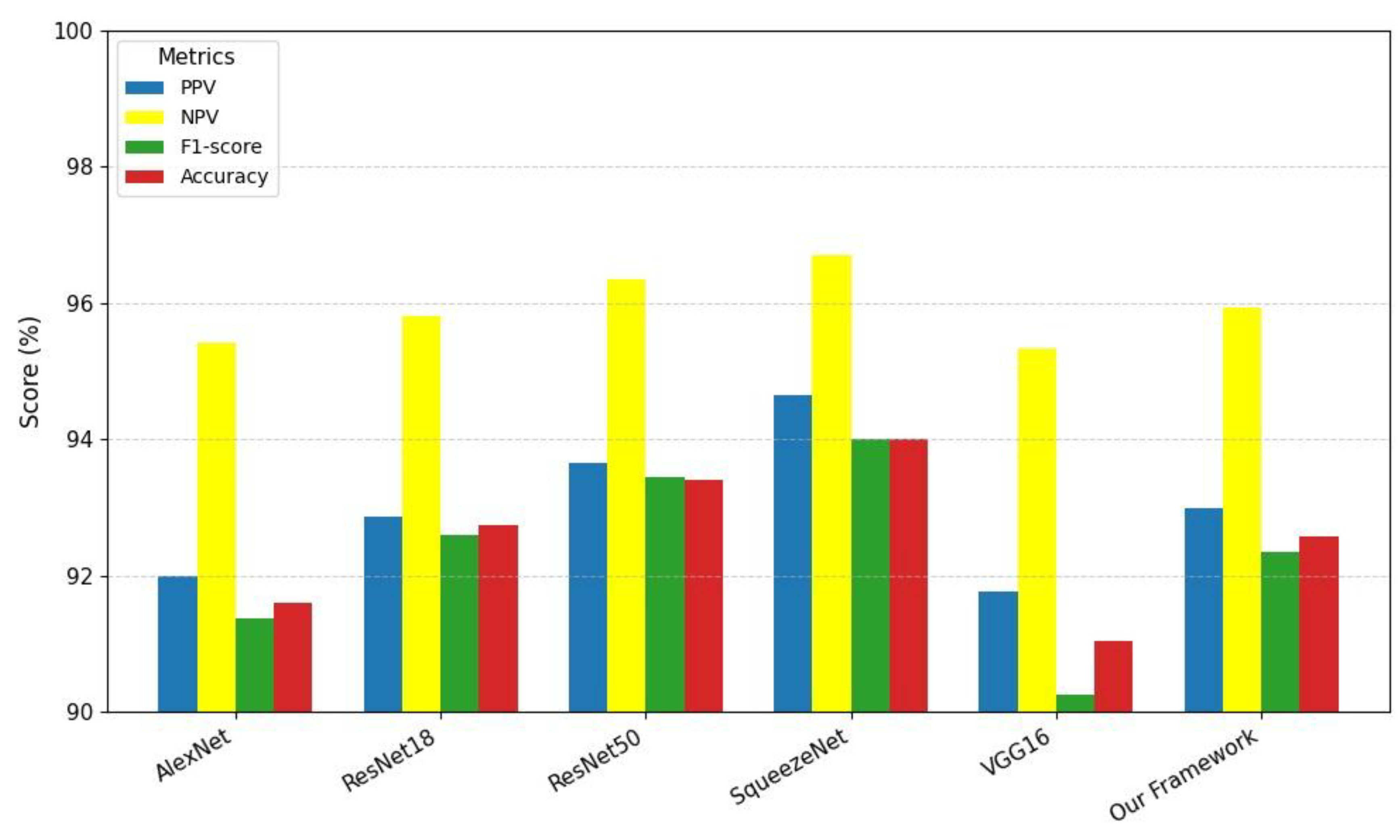
3.7. Comparison of the Proposed Study with Other Techniques
3.8. Main Findings
3.9. Limitations and Future Recommendations
4. Conclusions
References
- Binny, R.N.; et al. Sensitivity of reverse transcription polymerase chain reaction tests for severe acute respiratory syndrome coronavirus 2 through time. The Journal of infectious diseases, 2023, 227, 9–17. [Google Scholar] [CrossRef]
- Koh, H.K.; Geller, A.C.; VanderWeele, T.J. Deaths from COVID-19. Jama, 2021, 325, 133–134. [Google Scholar] [CrossRef]
- Eccleston, C.; et al. Managing patients with chronic pain during the COVID-19 outbreak: considerations for the rapid introduction of remotely supported (eHealth) pain management services. Pain, 2020, 161, 889–893. [Google Scholar] [CrossRef] [PubMed]
- Yuan, Y.; et al. The development of COVID-19 treatment. Frontiers in immunology, 2023, 14, 1125246. [Google Scholar] [CrossRef] [PubMed]
- Christie, A. Decreases in COVID-19 cases, emergency department visits, hospital admissions, and deaths among older adults following the introduction of COVID-19 vaccine—United States, September 6, 2020–May 1, 2021. MMWR. Morbidity and mortality weekly report, 2021, 70.
- Shereen, M.A.; et al. COVID-19 infection: Emergence, transmission, and characteristics of human coronaviruses. Journal of advanced research, 2020, 24, 91–98. [Google Scholar] [CrossRef] [PubMed]
- Dong, D.; et al. The role of imaging in the detection and management of COVID-19: a review. IEEE reviews in biomedical engineering, 2020, 14, 16–29. [Google Scholar] [CrossRef] [PubMed]
- Kolhar, M.; Al Rajeh, A.M.; Kazi, R.N.A. Augmenting Radiological Diagnostics with AI for Tuberculosis and COVID-19 Disease Detection: Deep Learning Detection of Chest Radiographs. Diagnostics, 2024, 14, 1334. [Google Scholar] [CrossRef]
- Jouibari, Z.E.; Moakhkhar, H.N.; Baleghi, Y. Emergency covid-19 detection from chest x-rays using deep neural networks and ensemble learning. Multimedia Tools and Applications, 2024, 83, 52141–52169. [Google Scholar] [CrossRef]
- Srinivas, K.; et al. COVID-19 prediction based on hybrid Inception V3 with VGG16 using chest X-ray images. Multimedia Tools and Applications, 2024, 83, 36665–36682. [Google Scholar] [CrossRef]
- Kumar, M.; SL, S.D.; Prashanth, B. CXNet-A Novel approach for COVID-19 detection and Classification using Chest X-Ray image. Procedia Computer Science, 2024, 235, 2486–2497. [Google Scholar]
- Fernández-Miranda, P.M.; et al. A retrospective study of deep learning generalization across two centers and multiple models of X-ray devices using COVID-19 chest-X rays. Scientific Reports, 2024, 14, 14657. [Google Scholar] [CrossRef] [PubMed]
- Brunese, L.; et al. Explainable deep learning for pulmonary disease and coronavirus COVID-19 detection from X-rays. Computer Methods and Programs in Biomedicine, 2020, 196, 105608. [Google Scholar] [CrossRef] [PubMed]
- Nayak, S.R.; et al. Application of deep learning techniques for detection of COVID-19 cases using chest X-ray images: A comprehensive study. Biomedical Signal Processing and Control, 2021, 64, 102365. [Google Scholar] [CrossRef]
- Zhang, J.; et al. Viral pneumonia screening on chest X-rays using confidence-aware anomaly detection. IEEE transactions on medical imaging, 2020, 40, 879–890. [Google Scholar] [CrossRef]
- Arias-Londono, J.D.; et al. Artificial intelligence applied to chest X-ray images for the automatic detection of COVID-19. A thoughtful evaluation approach. Ieee Access, 2020, 8, 226811–226827. [Google Scholar] [CrossRef]
- Vaid, S.; Kalantar, R.; Bhandari, M. Deep learning COVID-19 detection bias: accuracy through artificial intelligence. International Orthopaedics, 2020, 44, 1539–1542. [Google Scholar] [CrossRef]
- Kassania, S.H.; et al. Automatic detection of coronavirus disease (COVID-19) in X-ray and CT images: a machine learning based approach. Biocybernetics and Biomedical Engineering, 2021, 41, 867–879. [Google Scholar] [CrossRef] [PubMed]
- Hussain, E.; et al. CoroDet: A deep learning based classification for COVID-19 detection using chest X-ray images. Chaos, Solitons & Fractals, 2021, 142, 110495. [Google Scholar]
- Ismael, A.M.; Şengür, A. Deep learning approaches for COVID-19 detection based on chest X-ray images. Expert Systems with Applications, 2021, 164, 114054. [Google Scholar] [CrossRef]
- Xu, X.; et al. A deep learning system to screen novel coronavirus disease 2019 pneumonia. Engineering, 2020, 6, 1122–1129. [Google Scholar] [CrossRef]
- Ardakani, A.A.; et al. Application of deep learning technique to manage COVID-19 in routine clinical practice using CT images: Results of 10 convolutional neural networks. Computers in biology and medicine, 2020, 121, 103795. [Google Scholar] [CrossRef]
- Li, L.; et al. Artificial intelligence distinguishes COVID-19 from community acquired pneumonia on chest CT. Radiology, 2020, 200905.
- Çiçek, Ö.; et al. 3D U-Net: learning dense volumetric segmentation from sparse annotation. in International conference on medical image computing and computer-assisted intervention. 2016. Springer.
- Hu, R.; et al. Automated diagnosis of covid-19 using deep learning and data augmentation on chest ct. Medrxiv 2020, 2020.04. 24.20078998. [Google Scholar]
- Wang, L.; Lin, Z.Q.; Wong, A. Covid-net: A tailored deep convolutional neural network design for detection of covid-19 cases from chest x-ray images. Scientific reports, 2020, 10, 19549. [Google Scholar] [CrossRef]
- Butt, C.; et al. Deep learning system to screen coronavirus disease 2019 pneumonia. Appl Intell 2020. [Google Scholar]
- Bondugula, R.K.; Udgata, S.K.; Bommi, N.S. A novel weighted consensus machine learning model for covid-19 infection classification using CT scan images. Arabian Journal for Science and Engineering, 2023, 48, 11039–11050. [Google Scholar] [CrossRef]
- Sinra, A.; Angriani, H. Automated Classification of COVID-19 Chest X-ray Images Using Ensemble Machine Learning Methods. Indonesian Journal of Data and Science, 2024, 5, 45–53. [Google Scholar] [CrossRef]
- Hussein, A.M.; et al. Auto-detection of the coronavirus disease by using deep convolutional neural networks and X-ray photographs. Scientific reports, 2024, 14, 534. [Google Scholar] [CrossRef]
- Chen, T.; et al. A vision transformer machine learning model for COVID-19 diagnosis using chest X-ray images. Healthcare Analytics, 2024, 5, 100332. [Google Scholar] [CrossRef]
- Talukder, M.A.; et al. Empowering covid-19 detection: Optimizing performance through fine-tuned efficientnet deep learning architecture. Computers in Biology and Medicine, 2024, 168, 107789. [Google Scholar] [CrossRef] [PubMed]
- Bhatele, K.R.; et al. Covid-19 detection: A systematic review of machine and deep learning-based approaches utilizing chest x-rays and ct scans. Cognitive Computation, 2024, 16, 1889–1926. [Google Scholar] [CrossRef] [PubMed]
- Nair, S.S.K.; et al. CovMediScanX: A medical imaging solution for COVID-19 diagnosis from chest X-ray images. Journal of Medical Imaging and Radiation Sciences, 2024, 55, 272–280. [Google Scholar] [CrossRef]
- Yadlapalli, P.; Bhavana, D. Application of Fuzzy Deep Neural Networks for Covid 19 diagnosis through chest Radiographs. F1000Research, 2023, 12, 60. [Google Scholar] [CrossRef]
- Dokumacı, H.Ö. DERİN ÖĞRENME TABANLI MODELLERLE AKCİĞER X-RAY GÖRÜNTÜLERİNDEN COVID-19 TESPİTİ. Kahramanmaraş Sütçü İmam Üniversitesi Mühendislik Bilimleri Dergisi, 2024, 27, 481–487. [Google Scholar] [CrossRef]
- Rahman, T.; et al. Exploring the effect of image enhancement techniques on COVID-19 detection using chest X-ray images. Computers in biology and medicine, 2021, 132, 104319. [Google Scholar] [CrossRef]
- Chowdhury, M.E.; et al. Can AI help in screening viral and COVID-19 pneumonia? Ieee Access, 2020, 8, 132665–132676. [Google Scholar] [CrossRef]
- Gonzalez, R.C. Digital image processing. 2009: Pearson education india.
- Mallat, S. A wavelet tour of signal processing; Elsevier, 1999. [Google Scholar]
- Tomasi, C.; Manduchi, R. Bilateral Filtering for Gray and Color Images, in Proceedings of the Sixth International Conference on Computer Vision. 1998, IEEE Computer Society. p. 839.
- Nitish, S. Dropout: a simple way to prevent neural networks from overfitting. J. Mach. Learn. Res., 2014, 15, 1. [Google Scholar]
- Nwankpa, C.; et al. Activation functions: Comparison of trends in practice and research for deep learning. arXiv 2018, arXiv:1811.03378. [Google Scholar] [CrossRef]
- Agarap, A.F. Deep learning using rectified linear units (relu). arXiv 2018, arXiv:1803.08375. [Google Scholar]
- Jang, E.; Gu, S.; Poole, B. Categorical reparameterization with gumbel-softmax. arXiv 2016, arXiv:1611.01144. [Google Scholar]
- Smith, L.N. A disciplined approach to neural network hyper-parameters: Part 1--learning rate, batch size, momentum, and weight decay. arXiv arXiv:1803.09820, 2018.
- Akbar, S.; et al. Transitioning between convolutional and fully connected layers in neural networks. in Deep Learning in Medical Image Analysis and Multimodal Learning for Clinical Decision Support: Third International Workshop, DLMIA 2017, and 7th International Workshop, ML-CDS 2017, Held in Conjunction with MICCAI 2017, Québec City, QC, Canada, September 14, Proceedings 3. 2017. Springer.
- Yamashita, R.; et al. Convolutional neural networks: an overview and application in radiology. Insights into imaging, 2018, 9, 611–629. [Google Scholar] [CrossRef]
- Santurkar, S.; et al. How does batch normalization help optimization? Advances in neural information processing systems 2018, 31. [Google Scholar]
- Pérez, M. An Investigation of ADAM: A Stochastic Optimization Method, in Proceedings of the 39th International Conference on Machine Learning, Baltimore, Maryland, USA, PMLR 162, 2022. 2022. [Google Scholar]
- Klingler, N. AlexNet: A Revolutionary Deep Learning Architecture. viso. ai. https://viso. ai/deep-learning/alexnet/. Accessed, 2023. 13.
- Flach, P.; Kull, M. Precision-recall-gain curves: PR analysis done right. Advances in neural information processing systems 2015, 28. [Google Scholar]
- He, K.; et al. Deep residual learning for image recognition. in Proceedings of the IEEE conference on computer vision and pattern recognition. 2016.
- Iandola, F.N.; et al. SqueezeNet: AlexNet-level accuracy with 50x fewer parameters and. arXiv 2016, arXiv:1602.07360. [Google Scholar]
- Simonyan, K.; Zisserman, A. Very deep convolutional networks for large-scale image recognition. arXiv 2014, arXiv:1409.1556. [Google Scholar]
- Rainio, O.; Teuho, J.; Klén, R. Evaluation metrics and statistical tests for machine learning. Scientific Reports, 2024, 14, 6086. [Google Scholar] [CrossRef]
- Erickson, B.J.; Kitamura, F. Magician’s corner: 9. Performance metrics for machine learning models. Radiological Society of North America 2021, e200126. [Google Scholar] [CrossRef]
- Swift, A.; Heale, R.; Twycross, A. What are sensitivity and specificity? Evidence-Based Nursing, 2020, 23, 2–4. [Google Scholar] [CrossRef] [PubMed]
- Altman, D.G.; Bland, J.M. Diagnostic tests. 1: Sensitivity and specificity. BMJ: British Medical Journal, 1994, 308, 1552. [Google Scholar] [CrossRef]
- Miao, J.; Zhu, W. Precision–recall curve (PRC) classification trees. Evolutionary intelligence, 2022, 15, 1545–1569. [Google Scholar] [CrossRef]
- Derczynski, L. Complementarity, F-score, and NLP Evaluation. in Proceedings of the Tenth International Conference on Language Resources and Evaluation (LREC’16). 2016. [Google Scholar]
- Qureshi, S.A.; et al. SAlexNet: Superimposed AlexNet using residual attention mechanism for accurate and efficient automatic primary brain tumor detection and classification. Results in Engineering, 2025, 25, 104025. [Google Scholar]
- Samir, B.; et al. Deep learning for classification of chest X-ray images (Covid 19). arXiv 2023, arXiv:2301.02468. [Google Scholar] [CrossRef]
- Wang, S.; Ren, J.; Guo, X. A high-accuracy lightweight network model for X-ray image diagnosis: A case study of COVID detection. Plos one, 2024, 19, e0303049. [Google Scholar] [CrossRef]
- Singh, T.; et al. COVID-19 severity detection using chest X-ray segmentation and deep learning. Scientific Reports, 2024, 14, 19846. [Google Scholar] [CrossRef]
- Khan, M.A.; et al. COVID-19 classification from chest X-ray images: a framework of deep explainable artificial intelligence. Computational Intelligence and Neuroscience, 2022, 2022, 4254631. [Google Scholar] [CrossRef]
- Baker, M.; Buyya, R.; Laforenza, D. Grids and Grid technologies for wide-area distributed computing. Software: Practice and Experience, 2002, 32, 1437–1466. [Google Scholar] [CrossRef]
- Rouzrokh, P.; et al. Mitigating bias in radiology machine learning: 1. Data handling. Radiology: Artificial Intelligence, 2022, 4, e210290. [Google Scholar]
- Pennisi, M.; et al. An explainable AI system for automated COVID-19 assessment and lesion categorization from CT-scans. Artificial intelligence in medicine, 2021, 118, 102114. [Google Scholar] [CrossRef] [PubMed]
- Qureshi, S.A.; et al. Recent development of fluorescent nanodiamonds for optical biosensing and disease diagnosis. Biosensors, 2022, 12, 1181. [Google Scholar] [CrossRef]
- Qureshi, S.A.; et al. Radiogenomic classification for MGMT promoter methylation status using multi-omics fused feature space for least invasive diagnosis through mpMRI scans. Scientific reports, 2023, 13, 3291. [Google Scholar] [CrossRef] [PubMed]
- Qureshi, S.A.; et al. Intelligent ultra-light deep learning model for multi-class brain tumor detection. Applied Sciences, 2022, 12, 3715. [Google Scholar] [CrossRef]


| Feature | Dataset |
|---|---|
| Dataset name | C19 Radiography database |
| Year | 2020 |
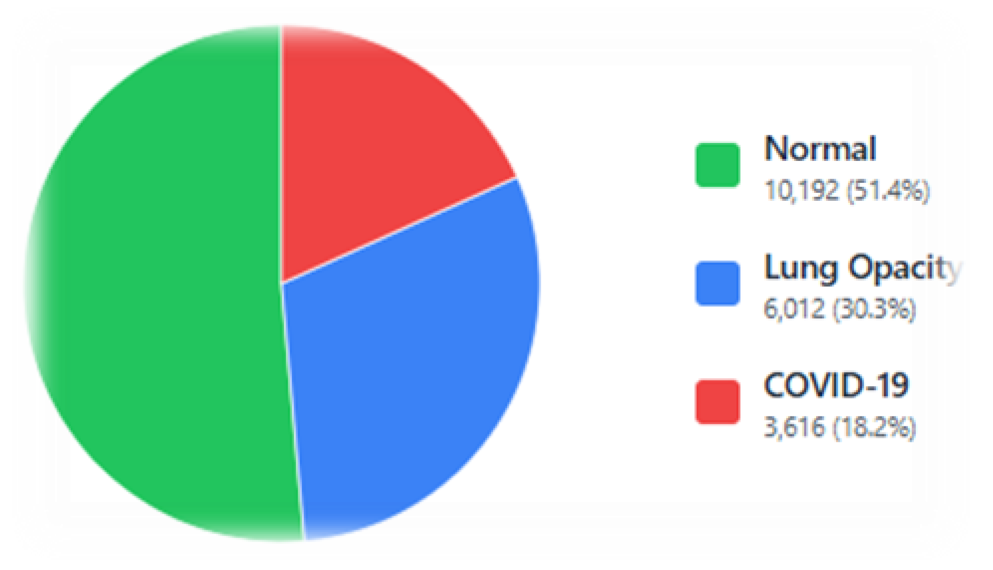
| Number of subjects | 3616 C19 patients |
| Availability | Publicly available |
| Site address | https://www.kaggle.com/datasets/tawsifurrahman/covid19-radiography-database |
| Type | Variation | Extreme Range / Value |
|---|---|---|
| Rotation | Clockwise / Anti-clockwise | ±10 degrees |
| Translation | Horizontal and Vertical shift | ±10% of image dimensions |
| Reflection | Horizontal (X-axis) | Random flip (p=0.5) |
| Affine | Random affine transformation | Translation only (no shear) |
| Parameter | Values under trial | Selected value |
|---|---|---|
| Learning rate | 0.0001, 0.001, 0.01,0.1 | 0.001 |
| Epochs | 1,5,10,15,20,25,30,40,50 | 30 |
| Minibatch (size) | 32,64 | 64 |
| Kernel depth | 64 | 64 |
| Kernel size | 3 × 3 | 3 × 3 |
| Activation | ReLU, Softmax | ReLU, Softmax |
| Pooling type | AvgPool, Max-Pool | AvgPool, Max-Pool |
| FC layers (fully connected) | 1,2 | 1 |
| Dropout | 0.3, 0.4, 0.5 | 0.5 |
| Solver name | ADAptive Moment estimation (ADAM) | ADAM |
| Parameter | Effect | Selected Value |
|---|---|---|
| D | Diameter of the pixel neighborhood. Larger values mean a stronger effect. | 9 |
| sigmaColor | Color differences affect filtering; a larger value means more smoothing. | 75 |
| sigmaSpace | How far in space does the filter look? Larger value considers more distant pixels. | 75 |
| Es | Sp (%) |
Rc/Sn (%) |
Pr/PPV (%) |
NPV (%) |
AUC (ROC) |
AUC (PR) |
F1-score (%) |
A (%) |
|---|---|---|---|---|---|---|---|---|
| 1 | 90.39±0.72 | 79.76±2.90 | 81.05±2.16 | 90.54±0.77 | 0.94±0.00 | 0.89±0.01 | 79.42±1.24 | 81.93±1.11 |
| 5 | 92.65±0.55 | 85.40±1.45 | 85.70±2.20 | 92.73±0.90 | 0.96±0.00 | 0.93±0.00 | 85.45±1.33 | 86.12±1.30 |
| 10 | 94.19±0.26 | 88.83±0.81 | 88.95±0.32 | 94.27±0.20 | 0.97±0.00 | 0.95±0.00 | 88.85±0.50 | 89.49±0.40 |
| 15 | 94.55±0.32 | 89.40±0.70 | 90.75±0.50 | 94.80±0.30 | 0.97±0.00 | 0.95±0.00 | 89.95±0.57 | 90.40±0.52 |
| 20 | 94.44±0.25 | 88.96±0.95 | 90.62±0.32 | 94.74±0.20 | 0.97±0.00 | 0.95±0.00 | 89.68±0.61 | 90.21±0.42 |
| 25 | 95.05±0.23 | 90.43±0.50 | 91.77±0.48 | 95.27±0.25 | 0.97±0.00 | 0.96±0.00 | 91.04±0.44 | 91.29±0.41 |
| 30 | 95.23±0.29 | 90.89±0.64 | 92.00±0.501 | 95.42±0.148 | 0.97±0.0 | 0.96±0.00 | 91.38±0.53 | 91.60±0.39 |
| 40 | 95.21±0.17 | 90.85±0.39 | 91.88±0.30 | 95.36±0.16 | 0.97±0.00 | 0.96±0.00 | 91.33±0.35 | 91.53±0.30 |
| 50 | 95.23±0.17 | 90.94±0.49 | 92.02±0.23 | 95.37±0.11 | 0.97±0.00 | 0.96±0.00 | 91.44±0.33 | 91.57±0.25 |
| Es | Sp (%) |
Rc/Sn (%) |
Pr/PPV (%) |
NPV (%) |
AUC (ROC) |
AUC (PR) |
F1-score (%) |
A (%) |
|---|---|---|---|---|---|---|---|---|
| 1 | 92.50±0.29 | 85.12±1.24 | 85.21±3.10 | 92.40±1.13 | 0.96±0.00 | 0.93±0.00 | 84.57±1.33 | 85.76±1.58 |
| 5 | 94.48±0.66 | 89.44±1.21 | 90.30±1.82 | 94.70±0.98 | 0.97±0.00 | 0.96±0.00 | 89.71±1.37 | 90.12±1.59 |
| 10 | 94.78±1.03 | 90.45±1.77 | 90.99±1.77 | 94.80±1.36 | 0.98±0.00 | 0.96±0.00 | 90.53±2.07 | 90.51±2.41 |
| 15 | 95.10±0.65 | 91.20±1.00 | 91.60±1.20 | 95.30±0.80 | 0.98±0.00 | 0.97±0.00 | 91.00±1.50 | 91.10±1.20 |
| 20 | 95.35±0.40 | 91.70±0.70 | 91.95±0.70 | 95.45±0.50 | 0.98±0.00 | 0.97±0.00 | 91.70±1.00 | 91.60±0.90 |
| 25 | 95.57±0.15 | 92.12±0.41 | 92.32±0.60 | 95.61±0.25 | 0.98±0.00 | 0.97±0.00 | 92.19±0.20 | 92.14±0.26 |
| 30 | 95.74±0.37 | 92.28±0.86 | 92.92±0.54 | 95.98±0.19 | 0.98±0.00 | 0.97±0.00 | 92.56±0.57 | 92.62±0.49 |
| 40 | 95.67±0.15 | 92.40±0.30 | 92.87±0.64 | 95.81±0.42 | 0.98±0.00 | 0.97±0.00 | 92.59±0.39 | 92.74±0.50 |
| 50 | 95.64±0.14 | 92.10±0.59 | 92.82±0.56 | 95.68±0.24 | 0.98±0.00 | 0.97±0.00 | 92.41±0.32 | 92.28±0.31 |
| Es | Sp (%) |
Rc/Sn (%) |
Pr/PPV (%) |
NPV (%) |
AUC (ROC) |
AUC ( PR) |
F1-score (%) |
A (%) |
|---|---|---|---|---|---|---|---|---|
| 1 | 92.43±1.52 | 85.55±2.60 | 84.81±4.08 | 92.04±2.18 | 0.96±0.00 | 0.94±0.00 | 84.30±4.33 | 85.17±4.28 |
| 5 | 94.76±0.15 | 90.00±0.43 | 90.18±1.38 | 94.80±0.55 | 0.98±0.00 | 0.96±0.00 | 89.94±0.61 | 90.44±0.61 |
| 10 | 95.28±0.26 | 90.89±0.93 | 92.40±0.45 | 95.75±0.18 | 0.98±0.00 | 0.96±0.00 | 91.54±0.44 | 91.92±0.29 |
| 15 | 95.75±0.21 | 92.03±0.59 | 92.88±0.21 | 95.95±0.07 | 0.98±0.00 | 0.97±0.00 | 92.43±0.38 | 92.57±0.25 |
| 20 | 95.98±0.13 | 92.69±0.32 | 93.25±0.70 | 96.21±0.31 | 0.98±0.00 | 0.97±0.00 | 92.93±0.21 | 93.00±0.26 |
| 30 | 96.24±0.09 | 93.24±0.30 | 93.66±0.25 | 96.36±0.10 | 0.98±0.00 | 0.97±0.00 | 93.44±0.13 | 93.41±0.12 |
| 40 | 96.06±0.19 | 92.96±0.54 | 93.48±0.20 | 96.21±0.11 | 0.98±0.00 | 0.97±0.00 | 93.21±0.34 | 93.13±0.27 |
| 50 | 95.99±0.18 | 92.77±0.60 | 93.48±0.33 | 96.16±0.12 | 0.98±0.00 | 0.97±0.00 | 93.11±0.44 | 93.04±0.29 |
| Es | Sp (%) |
Rc/Sn (%) |
Pr/PPV (%) |
NPV (%) |
AUC (ROC) |
AUC (PR) |
F1-score (%) |
A (%) |
|---|---|---|---|---|---|---|---|---|
| 20 | 96.25±0.88 | 93.41±1.44 | 94.26±2.08 | 96.51±1.3 | 98.9±0.07 | 98.31±0.17 | 93.49±2.01 | 93.48±2.10 |
| 25 | 96.52±0.37 | 93.95±0.72 | 94.65±0.9 | 96.71±0.59 | 98.94±0.13 | 98.36±0.21 | 94.01±0.81 | 94.01±0.85 |
| 30 | 96.63±0.6 | 94.18±1.04 | 93.97±2.73 | 96.64±1.04 | 98.91±0.15 | 98.32±0.24 | 93.95±1.65 | 93.95±1.69 |
| 40 | 95.98±1.3 | 92.18±3.72 | 94.57±1.21 | 96.65±0.75 | 98.77±0.36 | 98.12±0.51 | 93.32±2.08 | 93.39±1.98 |
| 50 | 90.78±0.43 | 80.04±0.76 | 81.00±1.23 | 90.53±0.66 | 0.94±0.00 | 0.89±0.00 | 80.03±1.04 | 82.24±1.22 |
| Es | Sp (%) |
Rc/Sn (%) |
Pr/PPV (%) |
NPV (%) |
AUC (ROC) |
AUC (PR) |
F1-score (%) |
A (%) |
|---|---|---|---|---|---|---|---|---|
| 1 | 90.43±1.25 | 79.04±3.99 | 81.36±0.89 | 91.47±0.89 | 0.93±0.02 | 0.93±0.12 | 82.12±2.99 | 83.12±1.70 |
| 5 | 91.43±1.14 | 81.04±3.67 | 86.36±0.81 | 92.41±0.85 | 0.96±0.01 | 0.92±0.01 | 82.37±2.96 | 84.87±1.70 |
| 10 | 92.10±0.90 | 82.50±2.80 | 87.50±0.70 | 93.00±0.80 | 0.96±0.00 | 0.93±0.01 | 83.90±2.20 | 86.00±1.30 |
| 15 | 92.75±0.65 | 83.80±2.00 | 88.25±0.60 | 93.60±0.60 | 0.96±0.00 | 0.93±0.01 | 85.25±1.80 | 87.20±1.00 |
| 20 | 93.00±0.40 | 84.60±1.30 | 89.00±0.40 | 93.85±0.45 | 0.96±0.00 | 0.94±0.00 | 86.20±1.20 | 87.90±0.70 |
| 25 | 93.05±0.35 | 85.00±1.10 | 89.40±0.30 | 93.90±0.35 | 0.96±0.00 | 0.94±0.00 | 86.60±1.00 | 88.10±0.60 |
| 30 | 93.11±0.30 | 85.40±0.98 | 89.79±0.19 | 94.02±0.27 | 0.97±0.00 | 0.94±0.00 | 87.14±0.76 | 88.33±0.53 |
| 40 | 94.62±0.11 | 88.76±0.47 | 91.63±0.25 | 95.27±0.09 | 0.97±0.00 | 0.95±0.00 | 90.01±0.24 | 90.82±0.14 |
| 50 | 94.83±0.22 | 89.11±0.69 | 91.77±0.33 | 95.34±0.16 | 0.98±0.00 | 0.96±0.00 | 90.26±0.54 | 91.04±0.37 |
| Method | Sp (%) |
Rc/Sn (%) |
Pr/PPV (%) |
NPV (%) |
AUC (ROC) |
AUC (PR) |
F1-score (%) |
A (%) |
|---|---|---|---|---|---|---|---|---|
| AlexNet | 95.23 | 90.89 | 92.00 | 95.42 | 0.97 | 0.96 | 91.38 | 91.60 |
| ResNet18 | 95.67 | 92.42 | 92.87 | 95.81 | 0.98 | 0.97 | 92.59 | 92.74 |
| ResNet50 | 96.24 | 93.24 | 93.66 | 96.36 | 0.98 | 0.97 | 93.44 | 93.41 |
| SqueezeNet | 96.52 | 93.95 | 94.65 | 96.71 | 0.98 | 0.98 | 94.01 | 94.01 |
| VGG16 | 94.83 | 89.11 | 91.77 | 95.34 | 0.98 | 0.96 | 90.26 | 91.04 |
| Method | Sp (%) |
Rc/Sn (%) |
Pr/PPV (%) |
NPV (%) |
AUC (ROC) |
AUC (PR) |
F1-score (%) |
A (%) |
|---|---|---|---|---|---|---|---|---|
| ResNet50 | 19.36 | 18.92 | 18.87 | 19.36 | 0.20 | 0.19 | 18.91 | 18.85 |
| ResNet18 | 19.13 | 18.58 | 18.55 | 19.14 | 0.20 | 0.19 | 18.57 | 18.58 |
| AlexNet | 18.95 | 17.97 | 18.20 | 18.98 | 0.19 | 0.19 | 18.09 | 18.13 |
| SqueezeNet | 19.47 | 19.21 | 19.27 | 19.50 | 0.20 | 0.20 | 19.14 | 19.10 |
| VGG16 | 18.79 | 17.28 | 18.11 | 18.95 | 0.20 | 0.19 | 17.65 | 17.91 |
| Optimized Results | 95.70 | 91.95 | 93.00 | 95.93 | 0.98 | 0.97 | 92.36 | 92.57 |
| Reference | Methodology | Data Split | Classes | A | Limitation(s) |
|---|---|---|---|---|---|
| [63] |
|
80/20 single split for both scenarios | 4 (C19, LO, N, VP) |
|
|
| [64] | MobileNetV3 + Dense Block | 5-Fold CV | 3 (C19, N, VP) |
|
|
| [65] | U-Net lung segmentation, Convolution-Capsule Network | 70% training, 15% validation, and 15% testing | 3 (C19, N, VP) |
(C19 86%, VP 93%, and N 85%) |
|
| [66] | Features from TL model, hybrid whale-elephant herding selection scheme, Extreme learning machine | Two partitions of 50% each, and 10-Fold CV on each of the partition | 4 (C19, N, LO, VP) |
|
|
| Proposed framework |
Ensemble of Transfer Learning | 5-Fold CV | 3(C19, N, LO) |
|
|
Disclaimer/Publisher’s Note: The statements, opinions and data contained in all publications are solely those of the individual author(s) and contributor(s) and not of MDPI and/or the editor(s). MDPI and/or the editor(s) disclaim responsibility for any injury to people or property resulting from any ideas, methods, instructions or products referred to in the content. |
© 2025 by the authors. Licensee MDPI, Basel, Switzerland. This article is an open access article distributed under the terms and conditions of the Creative Commons Attribution (CC BY) license (http://creativecommons.org/licenses/by/4.0/).


