Deep Learning Models for Multi-Class Pneumonia Detection in Chest X-Rays: A Comparative Study of VGG16, MobileNet, and ResNet152

1. Introduction

Pneumonia is an acute respiratory infection, mostly caused by viruses or bacteria. It can cause mild to life-threatening illness in people of all ages, but it is the largest single infectious cause of child mortality worldwide [1]. In recent years, the situation of pneumonia prevention and control has become more critical with the prevalence of several respiratory viruses, including SARS, H7N9, MERS and SARS-CoV-2 [2]. Medical imaging, especially chest X-ray, is an important tool to assist in the diagnosis of pneumonia [3]. Doctors can observe typical lesions in the lungs, such as map-like changes, gross glass shadows, and inflammatory infiltration of the lung parenchyma, through imaging, and these features help to quickly screen and diagnose patients with pneumonia. However, physicians referring to lung X-rays to screen for pneumonia may miss and misdiagnose the disease for a variety of reasons. Therefore, there is an urgent need for an accurate CAD method to detect pneumonia.

With the development of deep learning techniques, deep learning-based image classification tasks have shown great potential in the field of medical image analysis, especially the application of convolutional neural networks (CNNs) has made significant progress [4]. Some studies have analyzed binary classification of normal and pneumonia images, while others have investigated multi-class classification of normal images and different types of pneumonia, including viral and bacterial pneumonia infections [5].

VGG16, proposed by the Vision Geometry Group of the University of Oxford in 2014, is a deep convolutional neural network that achieved significant results in the ImageNet image classification task [6]. MobileNet, a lightweight CNN network proposed by the Google team in 2017, focuses on mobile or embedded devices [7]. ResNet152, a deep residual network proposed by Microsoft Research, introduces residual modules and bottleneck structures to enable the model to effectively learn image features at a deeper level [8].

ResNet152 excels in pneumonia diagnosis due to its 152-layer deep residual structure, which effectively captures complex features, prevents gradient vanishing, and boosts diagnostic accuracy and generalization. Unlike VGG16, which is parameter-heavy, inefficient, and prone to overfitting, or MobileNet, which is lightweight but less accurate and has limited feature extraction, our proposed ResNet152-based medical image segmentation framework aims to enhance pneumonia species recognition accuracy and efficiency. It leverages ResNet152’s deep residual learning to extract complex image features and optimizes performance through network fine-tuning.

2. Related Work

Based on recent advancements and comprehensive scholarly reviews, convolutional neural networks (CNNs) and transfer learning have emerged as pivotal tools in the field of medical imaging. CNNs possess powerful capabilities in extracting spatial hierarchies from image data, making them suitable for tasks like classification, detection, and segmentation. Transfer learning further enhances performance by leveraging pre-trained models, thus reducing the reliance on large annotated datasets.

Salehi et al. [9] provided an influential review emphasizing the advantages of CNNs and transfer learning in medical imaging. They noted that CNNs, particularly when combined with transfer learning strategies, can deliver superior diagnostic accuracy. However, they also highlighted key challenges such as small dataset sizes, model interpretability, and domain generalization. Similarly, Kundu et al. [10] introduced a CAD system using deep transfer learning for pneumonia detection via X-ray images. Their model achieved outstanding sensitivity and accuracy on public datasets like Kermany and RSNA, illustrating the clinical potential of pre-trained deep models.

To address temporal continuity in image sequences, Bai et al. [11] proposed integrating Fully Convolutional Networks (FCNs) with Recurrent Neural Networks (RNNs), significantly improving performance in segmenting aortic MR sequences. Meanwhile, Jha et al. [12] proposed DoubleU-Net—two stacked U-Net architectures—which enhanced contextual feature capture and outperformed traditional U-Net models.

Further advancing model efficiency, Li Gang et al. [13] introduced a MobileNetV1-based approach enhanced with Multi-Scale Feature Fusion (MSFF) and dilated convolutions, achieving over 99% accuracy in CT-based honeycomb lung recognition. In brain imaging, Roy et al. [14] used ResNet-152 to classify Alzheimer’s disease, reaching 99.30% binary and 98.79% quaternary classification accuracy. Beyond medical imaging, CNN architectures have demonstrated utility across domains. Yang et al. [15] applied an improved VGG16 to classify 12 peanut species, achieving a 96.7% average accuracy.

These works collectively illustrate that CNNs and their improved variants, when paired with transfer learning or attention mechanisms, not only elevate model performance in complex image tasks but also facilitate their practical deployment in medical diagnostics, agriculture, and industrial inspection.

3. Pneumonia Classification and Recognition Model

3.1. Transfer Learning

Transfer learning utilizes pre-trained models from a source task to improve performance on a target task, enhancing generalization while reducing computational cost. In medical imaging, it has proven effective—for example, Chen et al.’s Med3D network achieved superior Dice scores and classification accuracy. In lung X-ray classification, the process involves preprocessing images, using a pre-trained CNN, freezing most layers, replacing fully connected layers, and fine-tuning new layers with a low learning rate. This strategy enables efficient adaptation and improved diagnostic accuracy with limited data.

3.2. Mathematical Principles of Three Models

3.2.1. VGG16

Convolution is one of the core operations of CNN. Assuming that the input is a 2D matrix (image), the convolution operation slides through each region of the input step by step with a small weight matrix (convolution kernel), weighting and summing the localizations and outputting the feature map.

The role of the maximum pooling layer is to downsample the feature map to reduce the spatial dimensions of the data while retaining the most important feature information. Maximum pooling typically uses a 2×2 window and slides in the stride of 2. This halves the size of the input feature map and reduces subsequent calculations.

VGG16 has 13 convolutional layers. After convolutional layers, three fully connected layers lead to the model’s predictions. Stacking small kernels increases depth and nonlinearity, reducing parameters and improving feature extraction and classification 5.

VGG16 is suitable for tasks such as image classification, target detection, and image segmentation, and is particularly good at migration learning, which enables it to quickly adapt to new tasks through fine-tuning. However, VGG16 has more parameters, resulting in a higher computational cost, but it is still a reliable choice.

3.2.2. MobileNet

MobileNet is based on Depthwise Separable Convolution, which decomposes traditional convolution into two steps: depth convolution and pointwise convolution, significantly reducing the amount of computation and model parameters.

Depthwise Convolution: Convolution operation is performed independently for each channel of the input feature map, without mixing information across channels. The size of the input feature map and the output feature map remains the same.

Pointwise Convolution: uses a 1×1 convolution kernel to linearly combine the outputs of deep convolution to increase the number of channels.

The MobileNetV1 starts from the input layer. It enters a stack of multiple depth-separable convolutional layers, gradually increasing the number of channels and reducing the spatial dimensionality. Finally, the network reduces the feature map to a one-dimensional vector through a global average pooling layer and then outputs the classification results through a fully connected layer.

Table 1. All layers of MobileNetV1 with specific parameters.

Layer	Type	Parameters	Input	Output	Activate
1	Convolutional	3×3, 32 filters, stride=2, padding=same	224×224×3	112×112×32	ReLU
2	Depthwise + Pointwise	Depthwise: 3×3, stride=1 Pointwise: 1×1, 64 filters	112×112×32	112×112×64	ReLU
3	Depthwise + Pointwise	Depthwise: 3×3, stride=2 Pointwise: 1×1, 128 filters	112×112×64	56×56×128	ReLU
4	Depthwise + Pointwise	Depthwise: 3×3, stride=1 Pointwise: 1×1, 128 filters	56×56×128	56×56×128	ReLU
5	Depthwise + Pointwise	Depthwise: 3×3, stride=2 Pointwise: 1×1, 256 filters	56×56×128	28×28×256	ReLU
6	Depthwise + Pointwise	Depthwise: 3×3, stride=1 Pointwise: 1×1, 256 filters	28×28×256	28×28×256	ReLU
7	Depthwise + Pointwise	Depthwise: 3×3, stride=2 Pointwise: 1×1, 512 filters	28×28×256	14×14×512	ReLU
8-12	Depthwise + Pointwise	Depthwise: 3×3, stride=1 Pointwise: 1×1, 512 filters	14×14×512	14×14×512	ReLU
13	Depthwise + Pointwise	Depthwise: 3×3, stride=2 Pointwise: 1×1, 1024 filters	14×14×512	7×7×1024	ReLU
14	Depthwise + Pointwise	Depthwise: 3×3, stride=2 Pointwise: 1×1, 1024 filters	7×7×1024	4×4×1024	ReLU
15	Average Pooling	4×4, stride=4	4×4×1024	1×1×1024	-
16	Fully Connected	1000 units	1×1×1024	1000	Softmax

Table 1. All layers of MobileNetV1 with specific parameters.

Layer	Type	Parameters	Input	Output	Activate
1	Convolutional	3×3, 32 filters, stride=2, padding=same	224×224×3	112×112×32	ReLU
2	Depthwise + Pointwise	Depthwise: 3×3, stride=1 Pointwise: 1×1, 64 filters	112×112×32	112×112×64	ReLU
3	Depthwise + Pointwise	Depthwise: 3×3, stride=2 Pointwise: 1×1, 128 filters	112×112×64	56×56×128	ReLU
4	Depthwise + Pointwise	Depthwise: 3×3, stride=1 Pointwise: 1×1, 128 filters	56×56×128	56×56×128	ReLU
5	Depthwise + Pointwise	Depthwise: 3×3, stride=2 Pointwise: 1×1, 256 filters	56×56×128	28×28×256	ReLU
6	Depthwise + Pointwise	Depthwise: 3×3, stride=1 Pointwise: 1×1, 256 filters	28×28×256	28×28×256	ReLU
7	Depthwise + Pointwise	Depthwise: 3×3, stride=2 Pointwise: 1×1, 512 filters	28×28×256	14×14×512	ReLU
8-12	Depthwise + Pointwise	Depthwise: 3×3, stride=1 Pointwise: 1×1, 512 filters	14×14×512	14×14×512	ReLU
13	Depthwise + Pointwise	Depthwise: 3×3, stride=2 Pointwise: 1×1, 1024 filters	14×14×512	7×7×1024	ReLU
14	Depthwise + Pointwise	Depthwise: 3×3, stride=2 Pointwise: 1×1, 1024 filters	7×7×1024	4×4×1024	ReLU
15	Average Pooling	4×4, stride=4	4×4×1024	1×1×1024	-
16	Fully Connected	1000 units	1×1×1024	1000	Softmax

MobileNet offers high performance with low latency and computational cost, making it ideal for tasks like image classification, object detection, and semantic segmentation. Though its accuracy might be slightly lower than larger models, its design excels in mobile and embedded applications.

3.2.3. Resnet152

The mathematics of ResNet152 is based on residual learning: assuming that the input is $x$ and the output is $f\left(x\right)$, ResNet enables the network to learn the difference between the input and the output more efficiently by learning the residual function $R\left(x\right)=f\left(x\right)-x$.

ResNet152 is designed based on the residual learning framework and aims to solve the problem of gradient vanishing and gradient explosion in deep network training by introducing skip connections to ensure the training efficiency of the network.

ResNet152 consists of 152 layers, starting with a 7×7 convolutional layer with stride 2 for downsampling. It is followed by four stages with multiple residual units. Feature map sizes are halved and channel numbers increased in each stage using stride-2 convolutions. The network ends with a global average pooling layer and a fully connected layer for classification

Table 2. All layers of Resnet152 with specific parameters.

LAYER	TYPE	PARAMETERS	INPUT	OUTPUT	ACTIVATE
1	Convolutional	7×7, 64 filters, stride=2, padding=same	224×224×3	112×112×64	2
2	Max Pooling	3×3, stride=2, padding=same	112×112×64	56×56×64	2
3-4	Residual Block (×3)	3×3, 64 filters, stride=1	56×56×64	56×56×64	1
5-14	Residual Block (×4)	3×3, 128 filters, stride=2 (first block)	56×56×64	28×28×128	2/1
15-34	Residual Block (×6)	3×3, 256 filters, stride=2 (first block)	28×28×128	14×14×256	2/1
35-50	Residual Block (×3)	3×3, 512 filters, stride=2 (first block)	14×14×256	7×7×512	2/1
51	Average Pooling	7×7, stride=1	7×7×512	1×1×512	1
52	Fully Connected	1000 units	1×1×512	1000	-

Table 2. All layers of Resnet152 with specific parameters.

LAYER	TYPE	PARAMETERS	INPUT	OUTPUT	ACTIVATE
1	Convolutional	7×7, 64 filters, stride=2, padding=same	224×224×3	112×112×64	2
2	Max Pooling	3×3, stride=2, padding=same	112×112×64	56×56×64	2
3-4	Residual Block (×3)	3×3, 64 filters, stride=1	56×56×64	56×56×64	1
5-14	Residual Block (×4)	3×3, 128 filters, stride=2 (first block)	56×56×64	28×28×128	2/1
15-34	Residual Block (×6)	3×3, 256 filters, stride=2 (first block)	28×28×128	14×14×256	2/1
35-50	Residual Block (×3)	3×3, 512 filters, stride=2 (first block)	14×14×256	7×7×512	2/1
51	Average Pooling	7×7, stride=1	7×7×512	1×1×512	1
52	Fully Connected	1000 units	1×1×512	1000	-

ResNet152 has a wide range of applicability and is particularly suitable for image classification tasks that require high accuracy, such as classification on large-scale image datasets or as a feature extractor for target detection and semantic segmentation.

4. Results

4.1. Dataset

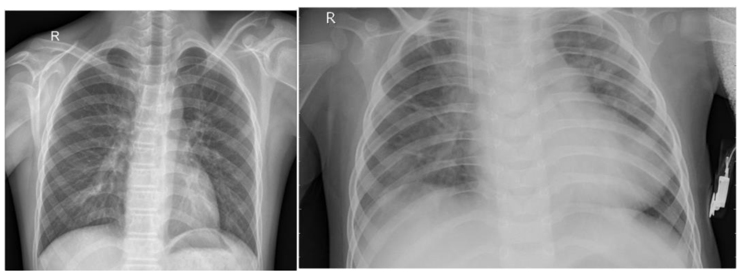
The chest X-ray dataset comprises 5,863 JPEG images collected from a Guangzhou medical center between 2010 and 2021 as part of routine clinical care. Images are categorized into pneumonia and normal classes and organized into train, test, and validation folders. To improve data quality, preprocessing included resizing to (224, 224, 3), normalization, denoising, label encoding, and data augmentation techniques such as rotation, scaling, shifting, shearing, and flipping, ensuring enhanced image quality and robustness for pneumonia classification tasks.

Figure 1. Sample Example of Dataset.

Figure 1. Sample Example of Dataset.

4.2. Comparison and Analysis of Results

4.2.1. VGG16

The VGG16 model performs well on the COVID category, but the recognition ability on the Normal and Viral Pneumonia categories needs to be improved, especially the recall of the Viral Pneumonia category is low. The overall accuracy is 80%; however, from the loss and accuracy curves, the model starts to show a slight overfitting phenomenon after about the 10th epoch, the training loss continues to decrease while the validation loss starts to fluctuate and increase, the training accuracy increases while the validation accuracy fluctuates.

Table 3. Test results of VGG16.

	Precision	Recall	F1-score	Support
Covid	0.93	1.00	0.96	26
Normal	0.68	0.85	0.76	20
Viral Pneumonia	0.77	0.50	0.61	20
Accuracy			0.80	66
Macro avg	0.79	0.78	0.77	66
Weighted avg	0.80	0.80	0.79	66

Table 3. Test results of VGG16.

	Precision	Recall	F1-score	Support
Covid	0.93	1.00	0.96	26
Normal	0.68	0.85	0.76	20
Viral Pneumonia	0.77	0.50	0.61	20
Accuracy			0.80	66
Macro avg	0.79	0.78	0.77	66
Weighted avg	0.80	0.80	0.79	66

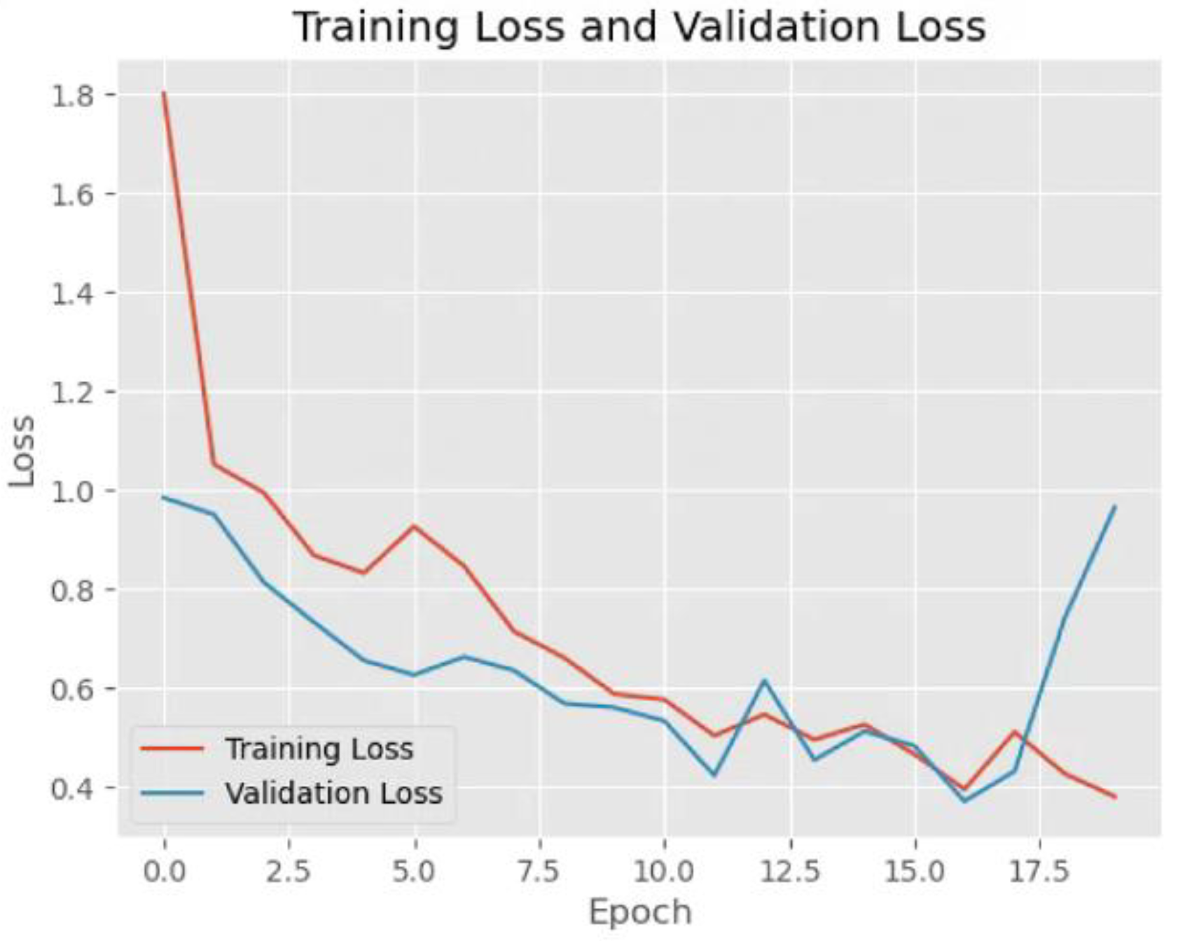
The Figure 2 presents a graph illustrating the concept of overfitting during model training. The x-axis represents the epoch, which refers to the number of times the model has gone through the entire training data. The y-axis represents loss, a measure of how much error the model makes in its predictions. The blue curve, labeled validation loss, decreases steadily as the number of training steps increases. This indicates that the model is improving on the data it has seen before. The red curve, labeled training loss, initially follows a similar downward trend but starts increasing after about 15.0 epochs. This suggests that the model is no longer generalizing well to unseen data. This figure demonstrates a key challenge in machine learning: the balance between learning useful patterns and overfitting to specific examples. Proper techniques, such as regularization, can help prevent overfitting and improve the model’s real-world performance.

Figure 2. Training and validation loss of VGG16.

Figure 2. Training and validation loss of VGG16.

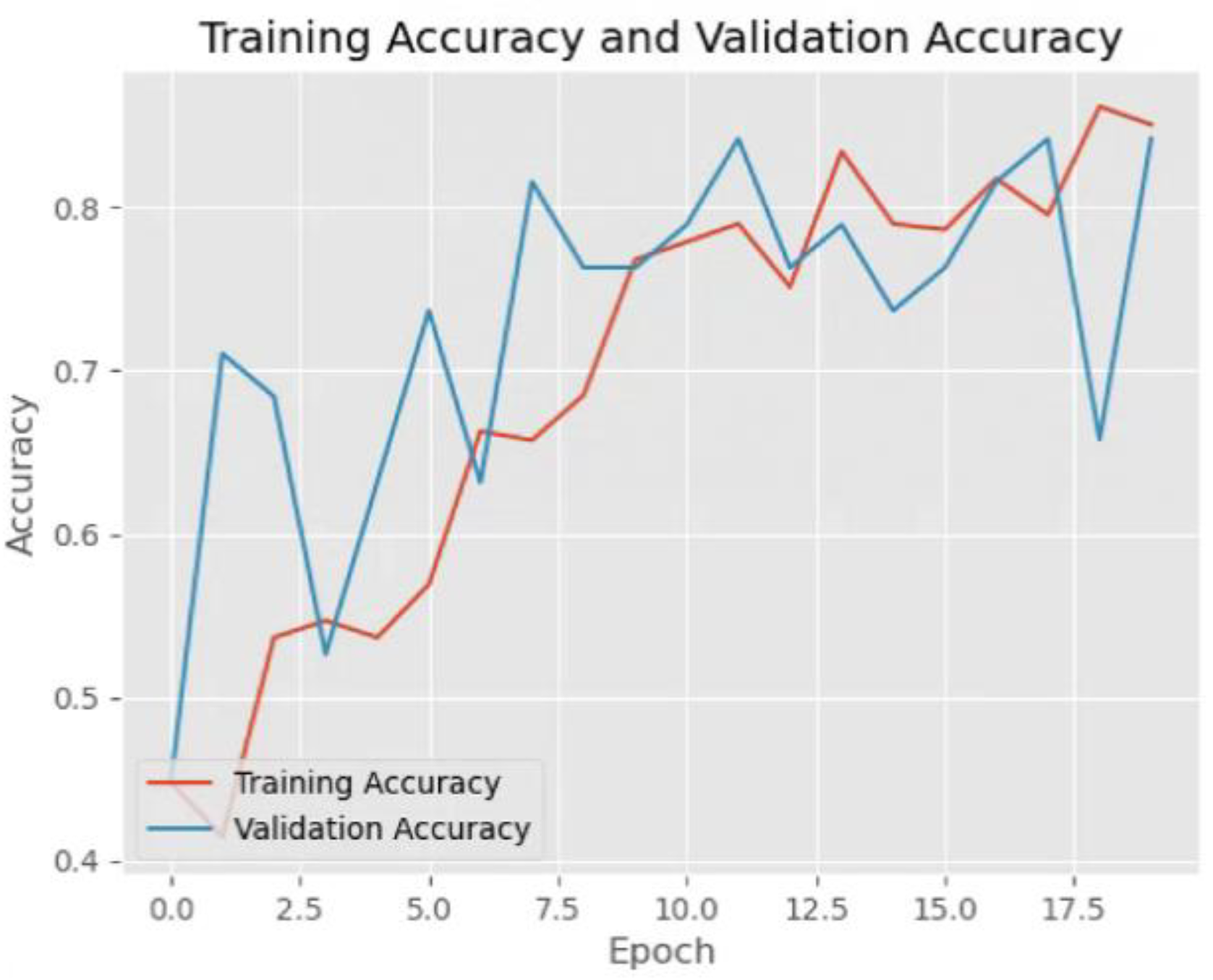
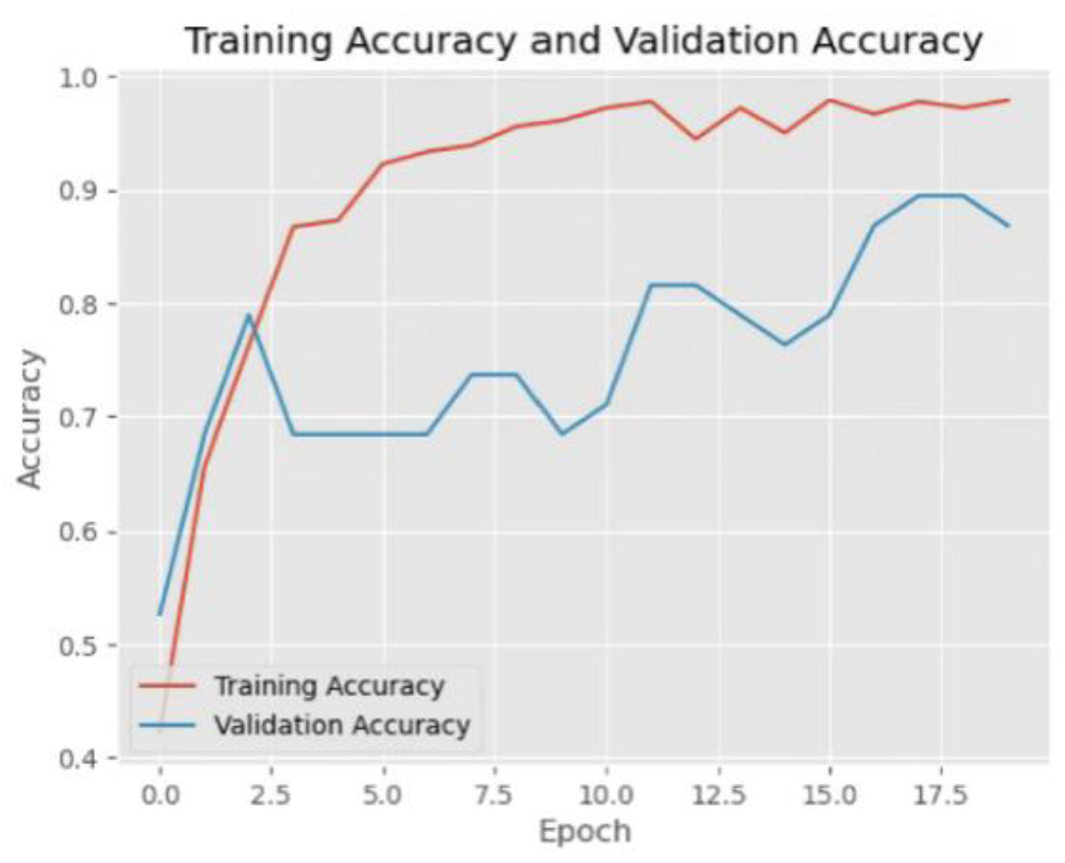
The Figure 3 presents a graph illustrating the improvement of model performance during training. The x-axis represents the epoch, which refers to the number of times the model has gone through the entire training dataset. The y-axis represents accuracy, a measure of how often the model makes correct predictions. The blue curve, labeled validation accuracy, increases steadily as the number of training steps increases. This indicates that the model is becoming better at making predictions on unseen data. The red curve, labeled training accuracy, also follows an upward trend and typically stays above the validation accuracy throughout training. This suggests that the model is effectively learning patterns in the training data while maintaining good generalization. This figure demonstrates a desirable outcome in machine learning: continuous improvement in both training and validation accuracy. Proper techniques, such as careful model tuning and diverse training data, can help sustain this positive trend and lead to better model performance in real-world applications.

Figure 3. Training accuracy and validation accuracy of VGG16.

Figure 3. Training accuracy and validation accuracy of VGG16.

4.2.2. MobileNet

The MobileNet model performs well on the COVID category with a precision of 1.00, but has low recall on the Normal and Viral Pneumonia categories of 0.50, respectively, resulting in overall F1 scores and accuracies of 0.65 and 0.65, respectively, suggesting that the model has some difficulty recognizing these categories. Although the training loss and validation loss decreased with increasing epoch and both the training accuracy and validation accuracy increased, the validation accuracy fluctuated and was relatively low.

Table 4. Test results of MobileNet.

	Precision	Recall	F1-score	Support
Covid	1.00	0.50	0.67	26
Normal	0.83	0.50	0.62	20
Viral Pneumonia	0.49	1.00	0.66	20
Accuracy			0.65	66
Macro avg	0.77	0.67	0.65	66
Weighted avg	0.79	0.65	0.65	66

Table 4. Test results of MobileNet.

	Precision	Recall	F1-score	Support
Covid	1.00	0.50	0.67	26
Normal	0.83	0.50	0.62	20
Viral Pneumonia	0.49	1.00	0.66	20
Accuracy			0.65	66
Macro avg	0.77	0.67	0.65	66
Weighted avg	0.79	0.65	0.65	66

4.2.3. Resnet152

The ResNet152 model showed good learning ability during the training process, with the training loss continuing to decrease and the training accuracy gradually increasing and approaching 1.0. The validation accuracy also fluctuated and tended to decrease after the initial rapid increase, which indicates that the model may be starting to overfit. The model performs well on the COVID and Viral Pneumonia categories, but there is some misclassification on the normal category. In general, the overall performance of the model is good.

Table 5. Test results of Resnet152.

	Precision	Recall	F1-score	Support
Covid	1.00	1.00	1.00	26
Normal	0.74	1.00	0.85	20
Viral Pneumonia	1.00	0.65	0.79	20
Accuracy			0.89	66
Macro avg	0.91	0.88	0.88	66
Weighted avg	0.92	0.89	0.89	66

Table 5. Test results of Resnet152.

	Precision	Recall	F1-score	Support
Covid	1.00	1.00	1.00	26
Normal	0.74	1.00	0.85	20
Viral Pneumonia	1.00	0.65	0.79	20
Accuracy			0.89	66
Macro avg	0.91	0.88	0.88	66
Weighted avg	0.92	0.89	0.89	66

All three models, VGG16, MobileNet and ResNet152, performed well on the COVID category, but there were differences in performance on the Normal and Viral Pneumonia categories. In contrast, the ResNet152 model performs better on all categories, especially achieving high precision and recall on the COVID and Viral Pneumonia categories, with an overall accuracy of 89%, showing better classification performance and generalization ability.

Figure 4. Training and validation loss of Resnet152.

Figure 4. Training and validation loss of Resnet152.

Figure 5. Training accuracy and validation accuracy of Resnet152.

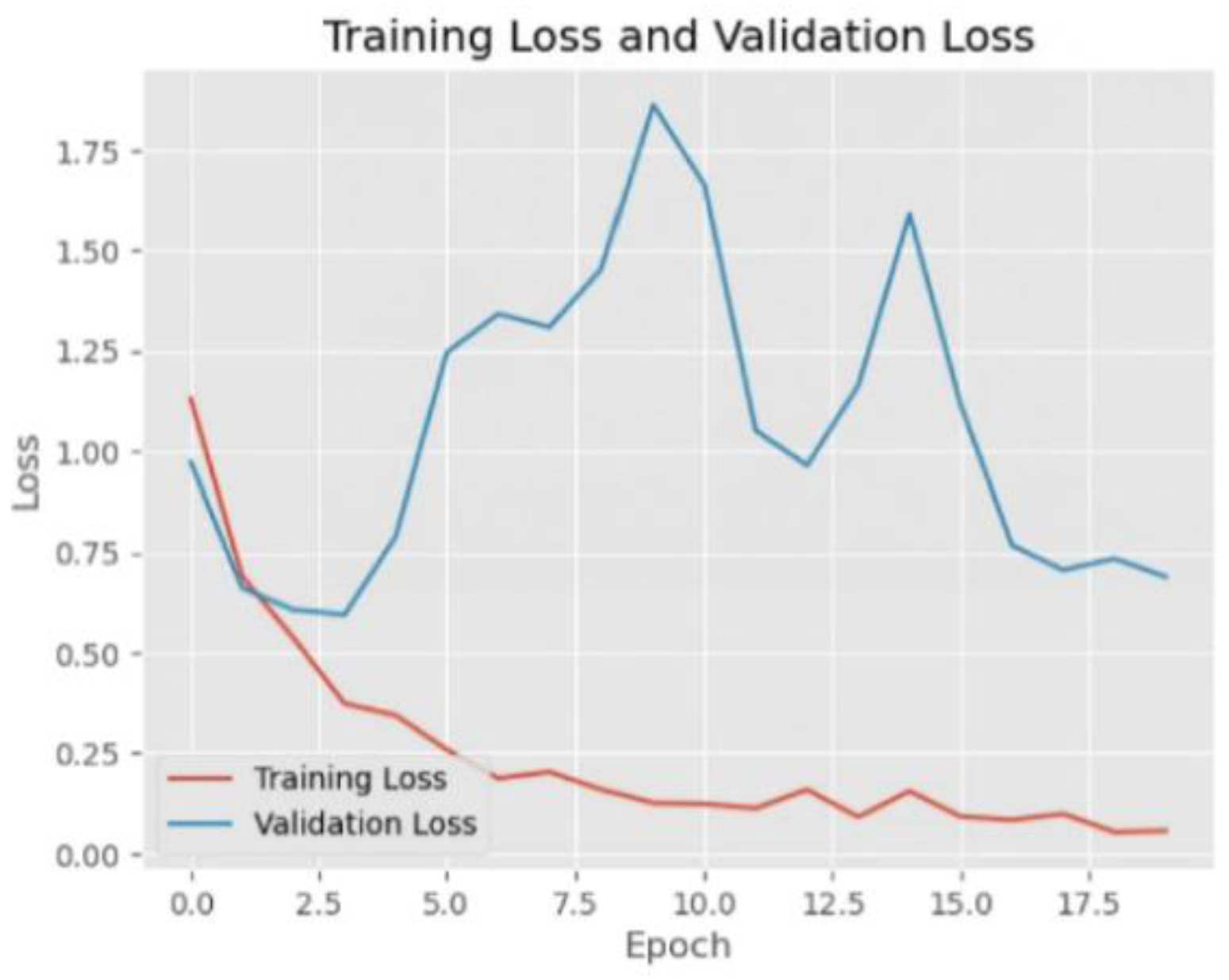
Figure 5. Training accuracy and validation accuracy of Resnet152.

5. Conclusions

This study systematically compared three deep learning models—VGG16, MobileNet, and ResNet152—for multi-class pneumonia classification using chest X-ray images. Experimental results demonstrate that ResNet152 achieved superior performance, with an overall accuracy of 89%. It attained perfect precision and recall (100%) in detecting COVID-19 and viral pneumonia, underscoring its strong diagnostic capability. This performance is attributed to its deep residual architecture, which effectively captures hierarchical features and mitigates gradient vanishing. However, classification performance for normal samples was suboptimal, with ResNet152 achieving only 74% accuracy, highlighting the challenge in distinguishing normal from pathological cases.

The study confirms that deep residual networks like ResNet152 are well-suited for complex medical imaging tasks and provides a benchmark framework for developing automated diagnostic tools to assist radiologists. Moreover, the approach can be extended to other similar tasks such as tuberculosis or lung cancer detection, accelerating AI integration into healthcare applications.

Despite the significant findings of this study, several limitations remain. First, the model relies on a relatively small, single-center, and retrospective dataset, which may introduce sampling bias and limit the generalizability of the results. Additionally, the presence of class imbalance—particularly underrepresentation of certain categories like viral pneumonia—likely contributed to the uneven performance across classification tasks. To address these issues, future research should consider incorporating large-scale, multi-center, and more balanced datasets to validate the model and enhance its robustness across diverse clinical settings. Moreover, the development of model interpretability techniques and lightweight network architectures will be crucial for deploying deep learning models in real-time, resource-constrained clinical environments, ensuring both performance and practicality in real-world applications.

References

- Mani C, S. Acute pneumonia and its complications. Principles and practice of pediatric infectious diseases 2017, 238. [Google Scholar]
- Abdelrahman Z, Li M, Wang X. Comparative review of SARS-CoV-2, SARS-CoV, MERS-CoV, and influenza a respiratory viruses. Frontiers in immunolog 2020, 11, 552909. [CrossRef] [PubMed]
- Garg, M.; Prabhakar, N.; Kiruthika, P.; Agarwal, R.; Aggarwal, A.; Gulati, A.; Khandelwal, N. Imaging of Pneumonia: An Overview. Curr. Radiol. Rep. 2017, 5, 1–14. [Google Scholar] [CrossRef]
- Miotto R, Wang F, Wang S, et al. Deep learning for healthcare: review, opportunities and challenges. Briefings in bioinformatics 2018, 19, 1236–1246. [CrossRef] [PubMed]
- Siddiqi, R.; Javaid, S. Deep Learning for Pneumonia Detection in Chest X-ray Images: A Comprehensive Survey. J. Imaging 2024, 10, 176. [Google Scholar] [CrossRef] [PubMed]
- Simonyan K, Zisserman A. Very deep convolutional networks for large-scale image recognition. arXiv 2014, arXiv:1409.1556,.
- Howard A G, Zhu M, Chen B, et al. Mobilenets: Efficient convolutional neural networks for mobile vision applications. arXiv 2017, arXiv:1704.04861.
- He K, Zhang X, Ren S, et al. Deep residual learning for image recognition. In Proceedings of the IEEE conference on computer vision and pattern recognition, 2016; pp. 770-778.
- Salehi, A.W.; Khan, S.; Gupta, G.; Alabduallah, B.I.; Almjally, A.; Alsolai, H.; Siddiqui, T.; Mellit, A. A Study of CNN and Transfer Learning in Medical Imaging: Advantages, Challenges, Future Scope. Sustainability 2023, 15, 5930. [Google Scholar] [CrossRef]
- Kundu, R.; Das, R.; Geem, Z.W.; Han, G.-T.; Sarkar, R.; Damaševičius, R. Pneumonia detection in chest X-ray images using an ensemble of deep learning models. PLOS ONE 2021, 16, e0256630. [Google Scholar] [CrossRef] [PubMed]
- Bai W, Suzuki H, Qin C, et al. Recurrent neural networks for aortic image sequence segmentation with sparse annotations. In Proceedings of the Medical Image Computing and Computer Assisted Intervention–MICCAI 2018: 21st International Conference, Granada, Spain, 16–20 September 2018. Proceedings, Part IV 11. Springer International Publishing, 2018: pp. 586-594.
- Jha D, Riegler M A, Johansen D, et al. Doubleu-net: A deep convolutional neural network for medical image segmentation. In Proceedings of the 2020 IEEE 33rd International symposium on computer-based medical systems (CBMS), IEEE, 2020, pp. 558-564.
- Gang, L.; Haixuan, Z.; Linning, E.; Ling, Z.; Yu, L.; Juming, Z. Recognition of honeycomb lung in CT images based on improved MobileNet model. Med Phys. 2021, 48, 4304–4315. [Google Scholar] [CrossRef] [PubMed]
- Roy P, Chisty M M O, Fattah H M A. Alzheimer’s disease diagnosis from MRI images using ResNet-152 Neural Network Architecture. In Proceedings of the 2021 5th International Conference on Electrical Information and Communication Technology (EICT). IEEE, 2021: 1-6.
- Yang, H.; Ni, J.; Gao, J.; Han, Z.; Luan, T. A novel method for peanut variety identification and classification by Improved VGG16. Sci. Rep. 2021, 11, 1–17. [Google Scholar] [CrossRef] [PubMed]
Disclaimer/Publisher’s Note: The statements, opinions and data contained in all publications are solely those of the individual author(s) and contributor(s) and not of MDPI and/or the editor(s). MDPI and/or the editor(s) disclaim responsibility for any injury to people or property resulting from any ideas, methods, instructions or products referred to in the content. |
© 2025 by the authors. Licensee MDPI, Basel, Switzerland. This article is an open access article distributed under the terms and conditions of the Creative Commons Attribution (CC BY) license (http://creativecommons.org/licenses/by/4.0/).
Copyright: This open access article is published under a Creative Commons CC BY 4.0 license, which permit the free download, distribution, and reuse, provided that the author and preprint are cited in any reuse.