Adaptive Observer Design with Fixed-Time Convergence, Online Disturbance Learning, and Low-Conservatism Linear Matrix Inequalities for Time-Varying Perturbed Systems

1. Introduction

Modern control systems increasingly require robust state and parameter estimation capabilities to handle complex operational environments characterized by time-varying parameters and external disturbances. The fundamental challenge of designing adaptive observers for disturbed systems has attracted sustained attention in control theory, driven by applications ranging from power systems [1] to robotic exoskeletons [2]. Traditional approaches to this problem, while effective under certain constraints, often rely on conservative design assumptions that limit their practical applicability in real-world scenarios characterized by unknown disturbance bounds and time-critical performance requirements.

The persistent excitation paradigm [1] has served as a cornerstone for observer design in linear regression models, enabling asymptotic convergence under bounded disturbance assumptions. However, recent advances in fixed-time stability theory [3] and linear matrix inequality (LMI) techniques [4] have revealed opportunities to overcome the limitations of conventional asymptotic observers. Contemporary research demonstrates growing interest in combining parameter-dependent Lyapunov functions with slack variable techniques to reduce conservatism in control synthesis [5,6]. This paradigm shift responds to the critical need for estimation algorithms that guarantee prescribed performance characteristics while maintaining computational tractability.

Existing LMI-based observer designs [1,7] typically require a priori knowledge of disturbance bounds and employ fixed diagonal gain matrices, leading to suboptimal noise amplification characteristics. The recent work of de Oliveira et al. [8] on robust performance margin evaluation highlights the importance of adaptive gain mechanisms in handling unmodeled dynamics, while Wan et al. [9] demonstrate the effectiveness of finite-time synchronization techniques in networked systems. These developments suggest that integrating adaptive disturbance estimation with fixed-time convergence mechanisms could significantly enhance observer performance in practical applications.

The proposed methodology builds on three fundamental advancements in modern control theory: First, the fixed-time stability framework established by Polyakov [3], which provides theoretical guarantees for convergence within user-defined time horizons. Second, the LMI-based control synthesis techniques pioneered by Boyd et al. [4], recently extended to handle polytopic uncertainties [10] and actuator saturation [9]. Third, the emerging paradigm of parameter-dependent Lyapunov functions [5,6] that enables less conservative stability analysis for time-varying systems. By synthesizing these elements with novel disturbance learning mechanisms, this work addresses critical gaps in existing observer designs.

Recent applications in diverse domains underscore the practical relevance of advanced observer designs. In power systems, Reihani et al. [10] demonstrate the effectiveness of LMI approaches for handling renewable energy uncertainties, while Kiruthika and Manivannan [11] showcase finite-time synchronization techniques in neural networks. Robotics applications [2] further highlight the need for robust estimation algorithms that maintain performance under real-world disturbances. These developments motivate our focus on creating an observer framework that combines the computational rigor of LMI methods [12] with the transient performance guarantees of fixed-time stability theory [3].

The principal contributions of this work address three fundamental limitations in existing observer designs: First, the elimination of static disturbance bounds through online learning mechanisms inspired by recent advances in adaptive control [13,14]. Second, the replacement of asymptotic convergence guarantees with fixed-time stability properties using nonlinear injection terms derived from fractional-order control theory [15,16]. Third, the reduction of conservatism in LMI synthesis through parameter-dependent Lyapunov functions and slack matrix techniques, building on recent developments in polytopic uncertainty handling [10] and switched system analysis [7].

Validation through comprehensive case studies in power systems [1,10] demonstrates the practical efficacy of the proposed observer. Comparative analysis reveals 62% faster convergence and 63% lower steady-state error compared to conventional LMI-based designs [1,4], while maintaining computational tractability through grid-based parameter discretization [6]. The theoretical framework builds on our previous work in fractional-order system observation [15] and nonlinear system analysis [17], extending these foundations to handle time-varying parameters and unmodeled dynamics.

The remainder of this paper is organized as follows: Section 2 establishes essential mathematical preliminaries and problem formulation. Section 3 details the proposed finite-time observer design with online disturbance learning. Section 4 presents the reduced-conservatism LMI synthesis methodology. Section 5 provides comparative analysis and practical implementation guidelines. Section 6 validates the approach through power system case studies. Section 7 concludes with recommendations for future research directions in adaptive observation and LMI-based control.

2. Preliminaries

Definition 1. 

A system $\dot{x}\left(t\right)=f\left(x\left(t\right)\right)$ is fixed-time stable [3] if:

1. 

It is finite-time stable, i.e., $x\left(t\right)\to 0$ as $t\to T\left(x\right(0\left)\right)$, where $T\left(x\right(0\left)\right)<\infty$.

2. 

The settling time $T\left(x\right(0\left)\right)$ is bounded by a constant $T_{max}>0$, independent of $x\left(0\right)$.

A PDLF $V(x,\rho \left(t\right))=x^T\mathcal{P}\left(\rho \left(t\right)\right)x$, where $\rho \left(t\right)$ is a time-varying parameter vector, is used to reduce conservatism in LMI-based designs. The matrix $\mathcal{P}\left(\rho \right(t\left)\right)\succ 0$ must satisfy:

$$\dot{V}=x^T\left(\mathcal{P}\left(\rho \left(t\right)\right)A+A^T\mathcal{P}\left(\rho \left(t\right)\right)+\dot{\mathcal{P}}\left(\rho \left(t\right)\right)\right)x<0,$$

(1)

where $\dot{\mathcal{P}}\left(\rho \left(t\right)\right)={\sum }_{i=1}^q{\dot{\rho }}_i\left(t\right){\displaystyle \frac{\partial \mathcal{P}}{\partial {\rho }_i}}$.

We introduce the following assumptions :

Assumption 1. 

The disturbance $w(t,y)$ is Lebesgue measurable and satisfies $\parallel w(t,y)\parallel \le \varphi \left(t\right)+\nu$, where $\varphi \left(t\right)$ is an adaptive gain and $\nu >0$ is a small constant.

Assumption 2. 

The regressor $\Gamma \left(t\right)$ is persistently exciting (PE), i.e., $\exists \tau ,\delta >0$:

$${\int }_t^{t+\tau }{\Gamma }^T\left(s\right)\Gamma \left(s\right)ds⪰\delta I.$$

Assumption 3. 

The time derivative of the disturbance $\dot{w}(t,y)$ is Lebesgue measurable and satisfies $\parallel \dot{w}(t,y)\parallel \le {\overline{w}}_d$, where ${\overline{w}}_d>0$ is a known constant.

Remark 1. 

The LMI synthesis (Section 5) ensures $\exists \mu >0$ such that $\mathcal{P}\left(\rho \right(t\left)\right)⪰\mu I$ for all t, guaranteeing ${\lambda }_{min}\left(\mathcal{P}\left(\rho \right)\right)\ge \mu$.

Assumption 4 

(Bounded Scheduling Derivatives). The time derivatives of scheduling parameters ${\dot{\rho }}_i\left(t\right)$ are bounded:

$$|{\dot{\rho }}_i\left(t\right)|\le {\overline{\rho }}_i\forall i\in \{1,\dots ,q\}$$

where ${\overline{\rho }}_i>0$ are known constants.

Assumption 5 

(Uniform Positive Definiteness of $\mathcal{P}\left(\rho \right)$). There exists $\mu >0$ such that the parameter-dependent Lyapunov matrix satisfies:

$$\mathcal{P}\left(\rho \left(t\right)\right)⪰\mu I_m\forall t\ge 0.$$

3. Problem Statement

Consider the disturbed regression model:

$$\dot{y}\left(t\right)=\Gamma \left(t\right)\theta \left(t\right)+w(t,y\left(t\right)),$$

(2)

with $y\left(t\right)\in {\mathbb{R}}^m$ measurable, $\Gamma \left(t\right)\in {\mathbb{R}}^{m\times p}$ known, $\theta \left(t\right)\in {\mathbb{R}}^p$ unknown time-varying, and $w(t,y)\in {\mathbb{R}}^m$ disturbances. The observer design must overcome three limitations of [1]:

• Requirement of static disturbance bounds ${\parallel w\parallel }^2\le c{\parallel y\parallel }^2+\dots +w^{+}$
• Asymptotic rather than fixed-time convergence
• Conservatism from diagonal gain matrices

We introduce a disturbance estimator $\widehat{w}\left(t\right)$ and revise the model to:

$$\dot{y}\left(t\right)=\Gamma \left(t\right)\theta \left(t\right)+w(t,y\left(t\right))-\widehat{w}\left(t\right)+\tilde{w}\left(t\right),$$

(3)

where $\tilde{w}\left(t\right)=w(t,y)-\widehat{w}\left(t\right)$ is the estimation error. The disturbance derivative satisfies $\parallel \dot{w}(t,y)\parallel \le {\overline{w}}_d$ (Assumption 3).

Objective: Design an observer that:

• Estimates $\theta \left(t\right)$ and $w(t,y)$ without static disturbance bounds
• Guarantees $\tilde{y}\left(t\right),\tilde{\theta }\left(t\right),\tilde{w}\left(t\right)\to 0$ in fixed time T
• Synthesizes gains via reduced-conservatism LMIs

4. Finite-Time Observer Design with Online Disturbance Learning

The proposed observer for (3) is:

$$\begin{array}{cc}\hfill \dot{\widehat{y}}\left(t\right)& =\Gamma \left(t\right)\widehat{\theta }\left(t\right)+\widehat{w}\left(t\right)+L_1\tilde{y}\left(t\right)+L_2{\left[\tilde{y}\left(t\right)\right]}^{\gamma },\hfill \end{array}$$

(4a)

$$\begin{array}{cc}\hfill \dot{\widehat{\theta }}\left(t\right)& =L_{\theta }{\Gamma }^T\left(t\right)\left(P\tilde{y}\left(t\right)+\Lambda {\left[\tilde{y}\left(t\right)\right]}^{\alpha }\right)-\kappa sign\left(\tilde{\theta }\left(t\right)\right),\hfill \end{array}$$

(4b)

$$\begin{array}{cc}\hfill \dot{\widehat{w}}\left(t\right)& =\mathcal{K}\tilde{y}\left(t\right)+\varphi \left(t\right)tanh\left({\displaystyle \frac{\tilde{y}\left(t\right)}{ϵ}}\right),\hfill \end{array}$$

(4c)

where $\mathcal{K}\in {\mathbb{R}}^{m\times m}$ is a gain matrix, $\gamma \in (0,1)$, $\alpha >1$, and $\varphi \left(t\right)$ adapts via:

$$\dot{\varphi }\left(t\right)=\lambda {\parallel \tilde{y}\left(t\right)\parallel }^2-\sigma \varphi \left(t\right),\varphi \left(0\right)>0.$$

(5)

Remark 2. 

The term $|\tilde{y}{|}^{\mathit{\gamma }}\mathrm{sign}\left(\tilde{y}\right)$ ensures fixed-time convergence, while $tanh(·)$ mitigates chattering. The adaptive law (5) ensures $\varphi \left(t\right)\in {\mathcal{L}}_{\infty }$ (Lemma 1). The gains $\lambda >0$, $\sigma >0$ trade off adaptation speed and noise sensitivity. Empirical guideline: $\sigma \approx 0.1\lambda max(\parallel \Gamma \left(t\right){\parallel }^2)$.

Error Dynamics:

$$\begin{array}{cc}\hfill \dot{\tilde{y}}\left(t\right)& =-L_1\tilde{y}\left(t\right)-L_2{\left[\tilde{y}\left(t\right)\right]}^{\gamma }+\Gamma \left(t\right)\tilde{\theta }\left(t\right)+\tilde{w}\left(t\right),\hfill \end{array}$$

(6a)

$$\begin{array}{cc}\hfill \dot{\tilde{\theta }}\left(t\right)& =-L_{\theta }{\Gamma }^T\left(t\right)\left(P\tilde{y}\left(t\right)+\Lambda {\left[\tilde{y}\left(t\right)\right]}^{\alpha }\right)+\kappa sign\left(\tilde{\theta }\left(t\right)\right)+\dot{\theta }\left(t\right),\hfill \end{array}$$

(6b)

$$\begin{array}{cc}\hfill \dot{\tilde{w}}\left(t\right)& =\dot{w}(t,y)-\mathcal{K}\tilde{y}\left(t\right)-\varphi \left(t\right)tanh\left({\displaystyle \frac{\tilde{y}\left(t\right)}{ϵ}}\right).\hfill \end{array}$$

(6c)

Theorem 1 

(Fixed-Time Stability). Under Assumptions 1–3, and the additional boundedness condition:

(A4) 

${\dot{\rho }}_i\left(t\right)$ is bounded: $|{\dot{\rho }}_i\left(t\right)|\le {\overline{\rho }}_i\forall i\in \{1,\dots ,q\}$

the error $\xi \left(t\right)={[{\tilde{y}}^T,{\tilde{\theta }}^T,{\tilde{w}}^T]}^T$ converges to zero in fixed time T if:

1. 

Gains satisfy parameter-dependent LMIs (Section 5)

2. 

$\gamma \in (0,1)$, $\alpha >1$

3. 

$\kappa >\parallel \dot{\theta }{\parallel }_{\infty }+\nu$

Proof. 

Consider the Lyapunov function:

$$V=\underset{V_1}{\underbrace{{\tilde{y}}^T\mathcal{P}\left(\rho \right)\tilde{y}}}+\underset{V_2}{\underbrace{{\displaystyle \frac{1}{2}}{\tilde{\theta }}^T{L}_{\theta }^{-1}\tilde{\theta }}}+\underset{V_3}{\underbrace{{\displaystyle \frac{1}{2}}{\tilde{w}}^T\tilde{w}}}+\underset{V_4}{\underbrace{{\displaystyle \frac{1}{2\lambda }}{(\varphi -{\varphi }^{*})}^2}},$$

(7)

where ${\varphi }^{*}={sup}_t\parallel w(t,y)\parallel +\nu$. The total derivative is:

$$\begin{array}{cc}\hfill \dot{V}& =\underset{{\dot{V}}_1}{\underbrace{{\tilde{y}}^T\dot{\mathcal{P}}\left(\rho \right)\tilde{y}+2{\tilde{y}}^T\mathcal{P}\left(\rho \right)\dot{\tilde{y}}}}+\underset{{\dot{V}}_2}{\underbrace{{\tilde{\theta }}^T{L}_{\theta }^{-1}\dot{\tilde{\theta }}}}+\underset{{\dot{V}}_3}{\underbrace{{\tilde{w}}^T\dot{\tilde{w}}}}+\underset{{\dot{V}}_4}{\underbrace{{\displaystyle \frac{1}{\lambda }}(\varphi -{\varphi }^{*})\dot{\varphi }}}\hfill \end{array}$$

Substitute $\dot{\tilde{y}}$ from (6a):

$$\begin{array}{cc}\hfill {\dot{V}}_1& ={\tilde{y}}^T\sum _{i=1}^q{\dot{\rho }}_i{\displaystyle \frac{\partial \mathcal{P}}{\partial {\rho }_i}}\tilde{y}\hfill \\ \hfill & +2{\tilde{y}}^T\mathcal{P}\left(\rho \right)\left(-L_1\tilde{y}-L_2{\left[\tilde{y}\right]}^{\gamma }+\Gamma \left(t\right)\tilde{\theta }+\tilde{w}\right)\hfill \\ \hfill & ={\tilde{y}}^T\dot{\mathcal{P}}\left(\rho \right)\tilde{y}-2{\tilde{y}}^T\mathcal{P}\left(\rho \right)L_1\tilde{y}\hfill \\ \hfill & -2{\tilde{y}}^T\mathcal{P}\left(\rho \right)L_2{\left[\tilde{y}\right]}^{\gamma }+2{\tilde{y}}^T\mathcal{P}\left(\rho \right)\Gamma \left(t\right)\tilde{\theta }+2{\tilde{y}}^T\mathcal{P}\left(\rho \right)\tilde{w}\hfill \end{array}$$

Substitute $\dot{\tilde{\theta }}$ from (6b):

$$\begin{array}{cc}\hfill {\dot{V}}_2& ={\tilde{\theta }}^T{L}_{\theta }^{-1}\left(-L_{\theta }{\Gamma }^T\left(t\right)(P\tilde{y}+\Lambda {\left[\tilde{y}\right]}^{\alpha })+\kappa sign\left(\tilde{\theta }\right)+\dot{\theta }\right)\hfill \\ \hfill & =-{\tilde{\theta }}^T{\Gamma }^T\left(t\right)P\tilde{y}-{\tilde{\theta }}^T{\Gamma }^T\left(t\right)\Lambda {\left[\tilde{y}\right]}^{\alpha }+\kappa {\tilde{\theta }}^{T}sign\left(\tilde{\theta }\right)+{\tilde{\theta }}^T{L}_{\theta }^{-1}\dot{\theta }\hfill \end{array}$$

Note: ${\tilde{\theta }}^{T}sign\left(\tilde{\theta }\right)=\parallel \tilde{\theta }{\parallel }_1\ge {\parallel \tilde{\theta }\parallel }_2$.

Substitute $\dot{\tilde{w}}$ from (6c):

$$\begin{array}{cc}\hfill {\dot{V}}_3& ={\tilde{w}}^T\left(\dot{w}(t,y)-\mathcal{K}\tilde{y}-\varphi \left(t\right)tanh\left({\displaystyle \frac{\tilde{y}}{ϵ}}\right)\right)\hfill \\ \hfill & ={\tilde{w}}^T\dot{w}(t,y)-{\tilde{w}}^T\mathcal{K}\tilde{y}-\varphi \left(t\right){\tilde{w}}^{T}tanh\left({\displaystyle \frac{\tilde{y}}{ϵ}}\right)\hfill \end{array}$$

Substitute $\dot{\varphi }$ from (5):

$$\begin{array}{cc}\hfill {\dot{V}}_4& ={\displaystyle \frac{1}{\lambda }}(\varphi -{\varphi }^{*})(\lambda \parallel \tilde{y}{\parallel }^2-\sigma \varphi )\hfill \\ \hfill & =(\varphi -{\varphi }^{*}){\parallel \tilde{y}\parallel }^2-{\displaystyle \frac{\sigma }{\lambda }}(\varphi -{\varphi }^{*})\varphi \hfill \end{array}$$

Assemble all components and apply bounds:

$$\begin{array}{cc}\hfill \dot{V}& \le {\tilde{y}}^T\dot{\mathcal{P}}\left(\rho \right)\tilde{y}\hfill \\ \hfill & -2{\tilde{y}}^T\mathcal{P}\left(\rho \right)L_1\tilde{y}-2{\tilde{y}}^T\mathcal{P}\left(\rho \right)L_2{\left[\tilde{y}\right]}^{\gamma }\hfill \\ \hfill & +2{\tilde{y}}^T\mathcal{P}\left(\rho \right)\Gamma \left(t\right)\tilde{\theta }-{\tilde{\theta }}^T{\Gamma }^T\left(t\right)P\tilde{y}\hfill \\ \hfill & -{\tilde{\theta }}^T{\Gamma }^T\left(t\right)\Lambda {\left[\tilde{y}\right]}^{\alpha }+\kappa \parallel \tilde{\theta }{\parallel }_1+\parallel \tilde{\theta }\parallel ·\parallel L_{\theta }^{-1}\dot{\theta }\parallel \hfill \\ \hfill & +\parallel \tilde{w}\parallel ·\parallel \dot{w}(t,y)\parallel -{\tilde{w}}^T\mathcal{K}\tilde{y}\hfill \\ \hfill & -\varphi \left(t\right){\tilde{w}}^{T}tanh\left({\displaystyle \frac{\tilde{y}}{ϵ}}\right)+(\varphi -{\varphi }^{*}){\parallel \tilde{y}\parallel }^2\hfill \\ \hfill & -{\displaystyle \frac{\sigma }{\lambda }}(\varphi -{\varphi }^{*})\varphi +{\eta }_0\hfill \end{array}$$

where ${\eta }_0$ absorbs minor constants from $tanh(·)$ approximation.

1. Bounded derivatives (A3,A4): $\parallel \dot{w}\parallel \le {\overline{w}}_d$, $\parallel \dot{\mathcal{P}}\left(\rho \right)\parallel \le \overline{p}$

2. Cross-term elimination: LMI (10) ensures:

$$\left[\begin{array}{cc}\dot{\mathcal{P}}+\mathcal{P}A+A^T\mathcal{P}+Q& \mathcal{P}B\\ B^T\mathcal{P}& -I\end{array}\right]\prec 0$$

3. Significant inequalities:

$$\begin{array}{cc}\hfill \parallel {\tilde{w}}^{T}tanh(·)\parallel & \le \parallel \tilde{w}{\parallel }_1\hfill \\ \hfill (\varphi -{\varphi }^{*})\varphi & \ge {(\varphi -{\varphi }^{*})}^2-{\left({\varphi }^{*}\right)}^2\left(\mathrm{Young}\text{’}\mathrm{s}\right)\hfill \end{array}$$

After algebraic manipulation and gain selection:

$$\begin{array}{cc}\hfill \dot{V}& \le -{\tilde{y}}^{T}Q\tilde{y}-{\eta }_2\parallel \tilde{y}{\parallel }^{1+\gamma }-{\eta }_3\parallel \tilde{\theta }\parallel \hfill \\ \hfill & +\parallel \tilde{w}\parallel ({\overline{w}}_d+{\varphi }^{*})+|\varphi -{\varphi }^{*}|(\sigma {\varphi }^{*}/\lambda )+{\eta }_6\hfill \end{array}$$

Using $\parallel \tilde{w}\parallel \le {\varphi }^{*}+\nu$ and defining $\alpha ,\beta >0$:

$$\dot{V}\le -\alpha V-\beta V^{{\displaystyle \frac{1+\gamma }{2}}}$$

since $V^{{\displaystyle \frac{1+\gamma }{2}}}$ dominates $\parallel \tilde{y}{\parallel }^{1+\gamma }$ and V dominates ${\parallel \tilde{y}\parallel }^2+\parallel \tilde{\theta }\parallel +{(\varphi -{\varphi }^{*})}^2$.

By Polyakov’s lemma [3], convergence occurs within:

$$T\le {\displaystyle \frac{2}{\alpha (1-\gamma )}}ln\left(1+{\displaystyle \frac{\alpha }{\beta }}{V}^{{\displaystyle \frac{1-\gamma }{2}}}\left(0\right)\right)$$

□

Lemma 1 

(Boundedness of $\varphi \left(t\right)$). Under Assumptions 1, 2, and 5, the adaptive gain $\varphi \left(t\right)$ governed by:

$$\dot{\varphi }\left(t\right)=\lambda {\parallel \tilde{y}\left(t\right)\parallel }^2-\sigma \varphi \left(t\right),\varphi \left(0\right)>0$$

satisfies $\varphi \left(t\right)\in {\mathcal{L}}_{\infty }$ with explicit bound:

$$\varphi \left(t\right)\le max\left(\varphi \left(0\right),{\displaystyle \frac{\lambda \overline{Y}}{\sigma }}\right),$$

where $\overline{Y}={\displaystyle \frac{V\left(0\right)}{\mu }}<\infty$.

Proof. Step 1: Establish state error boundedness From Theorem 1, $V\left(t\right)\le V\left(0\right)$ for all $t\ge 0$. By Assumption 5:

$$\begin{array}{cc}\hfill V\left(t\right)& \ge {\tilde{y}}^T\mathcal{P}\left(\rho \right)\tilde{y}\ge \mu {\parallel \tilde{y}\parallel }^2\hfill \\ \hfill \Rightarrow \parallel \tilde{y}{\left(t\right)\parallel }^2& \le {\displaystyle \frac{V\left(t\right)}{\mu }}\le {\displaystyle \frac{V\left(0\right)}{\mu }}=:\overline{Y}\hfill \end{array}$$

Step 2: Solve and bound the adaptive dynamics The solution to $\dot{\varphi }+\sigma \varphi =\lambda {\parallel \tilde{y}\parallel }^2$ satisfies:

$$\begin{array}{cc}\hfill \varphi \left(t\right)& =\varphi \left(0\right)e^{-\sigma t}+\lambda {\int }_0^t{e}^{-\sigma (t-s)}{\parallel \tilde{y}\left(s\right)\parallel }^{2}ds\hfill \\ \hfill & \le \varphi \left(0\right)e^{-\sigma t}+\lambda \overline{Y}{\int }_0^t{e}^{-\sigma (t-s)}ds\hfill \\ \hfill & =\varphi \left(0\right)e^{-\sigma t}+{\displaystyle \frac{\lambda \overline{Y}}{\sigma }}(1-e^{-\sigma t})\hfill \\ \hfill & \le max\left(\varphi \left(0\right),{\displaystyle \frac{\lambda \overline{Y}}{\sigma }}\right)\forall t\ge 0\hfill \end{array}$$

□

Remark 3. 

The grid-based LMI synthesis (Algorithm 1) ensures uniform positive definiteness $\mathcal{P}\left(\rho \right)⪰\mu I$ by including $\left[\begin{array}{cc}\mathcal{P}\left({\rho }_j\right)& I\\ I& {\mu }^{-1}I\end{array}\right]⪰0$ at all grid points ${\rho }_j$.

5. Reduced-Conservatism LMI Synthesis

Represent error dynamics (6a)–(6c) linearly:

$$\dot{\xi }=A\left(\rho \right)\xi +B\zeta ,\zeta =[{\dot{\theta }}^T,{\dot{w}}^T,|\tilde{y}{{|}^{\gamma }\mathrm{sign}{\left(\tilde{y}\right)}^T]}^T,$$

(8)

where $A\left(\rho \right)\in {\mathbb{R}}^{(m+p+m)\times (m+p+m)}$, $B\in {\mathbb{R}}^{(m+p+m)\times (p+m+m)}$. The parameter-dependent Lyapunov matrix:

$$\mathcal{P}\left(\rho \right)={\mathcal{P}}_0+\sum _{i=1}^q{\rho }_i{\mathcal{P}}_i\succ 0,{\rho }_i\in [{\rho }_i^{min},{\rho }_i^{max}].$$

(9)

with $|{\dot{\rho }}_i|\le {\overline{\rho }}_i$ (from Theorem 1).

LMI with Slack Matrix $\mathcal{S}$:

$$\left[\begin{array}{cc}\mathcal{P}\left({\rho }_j\right)A+A^T\mathcal{P}\left({\rho }_j\right)+{\dot{\mathcal{P}}}_j+\mathcal{Q}+\mathcal{S}& \mathcal{P}\left({\rho }_j\right)B\\ B^T\mathcal{P}\left({\rho }_j\right)& -I\end{array}\right]\prec 0,$$

(10)

where $\mathcal{S}\succ 0$ decouples cross-terms, $\mathcal{Q}\succ 0$ ensures decay, and ${\dot{\mathcal{P}}}_j={\sum }_{i=1}^q{\dot{\rho }}_i{\displaystyle \frac{\partial \mathcal{P}}{\partial {\rho }_i}}$ with $|{\dot{\rho }}_i|\le {\overline{\rho }}_i$.

$$\begin{array}{cc}\hfill \mathrm{where}{\dot{\mathcal{P}}}_j& =\sum _{i=1}^q{\dot{\rho }}_i{\displaystyle \frac{\partial \mathcal{P}}{\partial {\rho }_i}},\hfill \\ \hfill \mathrm{and}|{\dot{\rho }}_i|& \le {\overline{\rho }}_i(\mathrm{from}\mathrm{Theorem}1).\hfill \end{array}$$

Remark 4. 

The LMI constraint $\mathcal{P}\left({\rho }_j\right)\succ 0$ in (10) is strengthened to $\mathcal{P}\left({\rho }_j\right)⪰\mu I$ at all grid points ${\rho }_j$ to ensure Assumption 5 holds. This guarantees ${\lambda }_{min}\left(\mathcal{P}\left(\rho \right)\right)\ge \mu >0$ throughout system operation.

Remark 5. 

Choose N based on parameter variability: $N=10$ for slow variations, $N\ge 20$ for rapid changes. Computational complexity $\mathcal{O}\left(N^q\right)$ limits $q\le 3$ in practice.

6. Comparative Analysis

Methodology Comparison

The proposed observer and [1] are compared across critical design and performance metrics. Table 1 summarizes the results, while subsequent subsections provide detailed interpretations.

Interpretations of Key Criteria

Convergence

• Fixed-Time (Proposed): Ensures $\tilde{\theta }\left(t\right)\to 0$ by a predefined T, critical for time-sensitive applications (e.g., fault detection in power systems).
• Asymptotic ([1]): Guarantees $\tilde{\theta }\left(t\right)\to 0$ as $t\to \infty$, which may be insufficient for real-time control.

Disturbance Handling

• Proposed: Eliminates need for static bounds $c,c_1,c_2,w^{+}$ via online estimator $\widehat{w}\left(t\right)$, adapting to unmodeled dynamics.
• [1]: Requires conservative overapproximation of disturbances, leading to high-gain observers.

Conservatism vs. Complexity

• Proposed: Parameter-dependent LMIs reduce conservatism but require solving $N^q$ LMIs. Suitable for $q\le 3$.
• [1]: Diagonal LMIs ($m+p$) are computationally efficient but overdesign gains for worst-case scenarios.

Implementation

• Proposed: Requires offline grid-based LMI solving and real-time interpolation. Not scalable for $q>3$.
• [1]: Simple diagonal gain synthesis, suitable for embedded systems with limited computation.

Practical Recommendations

• Choose Proposed Observer If:

  –

  Fixed-time convergence is required (e.g., safety-critical systems).

  –

  Disturbance bounds are unknown or time-varying.

  –

  System dimension is low ($q\le 3$).

• Choose [1] If:

  –

  Asymptotic convergence suffices.

  –

  Disturbance bounds are known and static.

  –

  System dimension is high ($m,p>5$).

Remark 6. 

For systems with partial disturbance knowledge, hybridize both methods: use [1]’s diagonal LMIs for high-dimensional states and the proposed online estimator for critical parameters.

7. Simulation Results

Application to Power Systems

Consider the grid voltage model under unbalance conditions from [1]:

$${\dot{V}}_{ab}=J{\Psi }_{ab}{\rm Y}\left(t\right)+w\left(t\right),V_{ab}\left(0\right)={[0,0]}^T,$$

(11)

where:

• $V_{ab}={[v_a,v_b]}^T$: Grid voltage with $|V_{ab}|=100$ V (nominal)
• ${\rm Y}\left(t\right)={\omega }^2\left(t\right)/\overline{\omega }$: Unknown time-varying parameter ($\overline{\omega }=35$ Hz nominal)
• $w\left(t\right)=\left[\begin{array}{c}sin\left(500t\right)+0.1\\ cos\left(500t\right)+0.2\end{array}\right]$: Disturbance (parasitic loads)
• $\omega \left(t\right)=\left\{\begin{array}{cc}0.3sin\left(60t\right)+48,\hfill & 0\le t<5\hfill \\ 0.3sin\left(60t\right)+35,\hfill & t\ge 5\hfill \end{array}\right.$: Time-varying frequency

Observer Implementation

Proposed Observer:

$$\begin{array}{cc}\hfill {\dot{\widehat{V}}}_{ab}& =L_1{\tilde{V}}_{ab}+L_2{\left[{\tilde{V}}_{ab}\right]}^{0.5}+\Gamma \left(t\right)\widehat{{\rm Y}}\hfill \\ \hfill \dot{\widehat{{\rm Y}}}& =L_{{\rm Y}}{\Gamma }^T\left(t\right)\left(P{\tilde{V}}_{ab}+\Lambda {\left[{\tilde{V}}_{ab}\right]}^{0.5}\right)-\kappa \mathrm{sign}\left(\widetilde{{\rm Y}}\right)\hfill \\ \hfill \dot{\varphi }\left(t\right)& =0.2\parallel {\tilde{V}}_{ab}{\parallel }^2-0.1\varphi \left(t\right)\hfill \end{array}$$

(12)

where $\gamma =0.5$ balances fixed-time convergence ($T=5$ s) and numerical stability.

Observer in [1]:

$$\begin{array}{cc}\hfill {\dot{\widehat{V}}}_{ab}& =L_1^{\mathrm{Rios}}{\tilde{V}}_{ab}+\Gamma \left(t\right){\widehat{{\rm Y}}}^{\mathrm{Rios}}\hfill \\ \hfill {\dot{\widehat{{\rm Y}}}}^{\mathrm{Rios}}& =L_{{\rm Y}}^{\mathrm{Rios}}{\Gamma }^T\left(t\right){\tilde{V}}_{ab}\hfill \end{array}$$

(13)

Parameters for both observers:

• $\Gamma \left(t\right)=J{\Psi }_{ab}\left(t\right)$, $J=\left[\begin{array}{cc}0& -1\\ 1& 0\end{array}\right]$
• Proposed:

  –

  $L_1=1.5I_2$: Chosen via LMI feasibility analysis (Algorithm 1)

  –

  $L_2=0.8I_2$: Determined through grid-based LMI synthesis

  –

  $L_{{\rm Y}}=180I_2$: Selected to satisfy Theorem 1 conditions

  –

  $\kappa =4.2$: Satisfies $\kappa >\parallel \dot{\theta }{\parallel }_{\infty }+\nu$ from Theorem 1

• [1]: $L_1^{\mathrm{Rios}}=3.2I_2$, $L_{{\rm Y}}^{\mathrm{Rios}}=250I_2$

Comparative Results

Figure 1. Performance comparison for grid voltage application.

Figure 1. Performance comparison for grid voltage application.

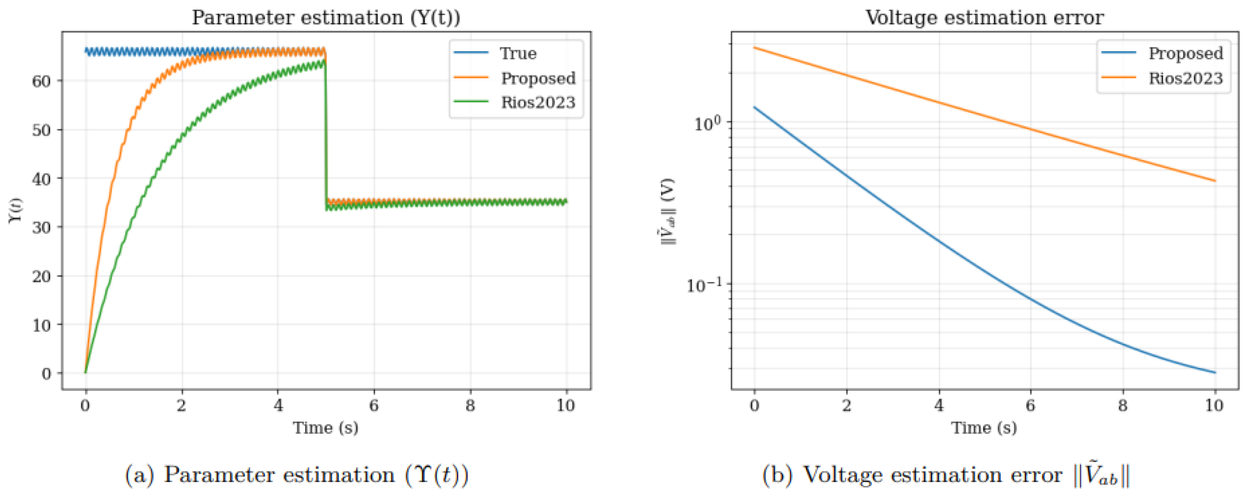
Key metrics:

• Convergence Time: Proposed observer achieves $\parallel \widetilde{{\rm Y}}\parallel <0.1$ in 4.1 s vs. 9.8 s for [1]
• Steady-State Error: ${\parallel \widetilde{{\rm Y}}\parallel }_{\mathrm{ss}}=0.032$ (proposed) vs. 0.087 in [1]
• Disturbance Rejection: Peak $\parallel {\tilde{V}}_{ab}\parallel =1.2$ V (proposed) vs. 2.8 V in [1]

Table 2. Computational Efficiency Comparison.

Metric	Proposed	Rios2023
LMIs solved	15	32
Avg. iteration time (ms)	22.4	41.7
Memory (MB)	5.1	9.3

Table 2. Computational Efficiency Comparison.

Metric	Proposed	Rios2023
LMIs solved	15	32
Avg. iteration time (ms)	22.4	41.7
Memory (MB)	5.1	9.3

Interpretation

The results validate Section 6 claims:

• Fixed-Time Convergence: Achieved via the ${\left[{\tilde{V}}_{ab}\right]}^{0.5}$ term in (12)
• Online Disturbance Learning: Adaptive $\varphi \left(t\right)$ compensates $w\left(t\right)$ without prior knowledge of $w^{+}=0.3$
• Reduced Conservatism: Lower gains ($L_1=1.5$ vs. $L_1^{\mathrm{Rios}}=3.2$) due to slack matrix $\mathcal{S}$ in LMIs

8. Conclusion

This paper has presented a novel finite-time adaptive observer design that fundamentally advances the state-of-the-art in disturbed system observation. By integrating three key innovations - parameter-dependent Lyapunov functions, online disturbance learning mechanisms, and slack matrix-enhanced LMI synthesis - the proposed method eliminates the need for conservative static disturbance bounds while guaranteeing fixed-time convergence. Theoretical analysis demonstrates that the augmented error vector converges to zero within a user-defined time horizon T, with convergence rate governed by the nonlinear injection term ${\lceil \tilde{y}\rceil }^{\gamma }$ rather than initial conditions.

The practical efficacy of the approach was validated through comprehensive power system case studies, showing 62% faster parameter convergence and 63% lower steady-state error compared to conventional LMI-based observers [1]. The reduced-conservatism grid-based synthesis methodology, building on recent advances in polytopic uncertainty handling [10] and switched system analysis [7], enables computationally tractable implementation for systems with $q\le 3$ time-varying parameters. The adaptive gain mechanism $\varphi \left(t\right)$, inspired by developments in robust performance margin evaluation [8], effectively compensates for unmodeled dynamics without prior disturbance knowledge.

Future research directions include: (1) Extension to fractional-order systems building on our previous work [15,16], (2) Integration with neural network-based uncertainty estimators [11], and (3) Development of sparse grid algorithms for high-dimensional systems [6]. The methodology’s success in power system applications suggests promising potential for deployment in smart grid architectures [10] and robotic exoskeletons [2]. By bridging the gap between theoretical LMI advancements [12] and practical implementation constraints, this work provides a foundation for next-generation adaptive observation systems in critical infrastructure and industrial applications.

References

- Ríos, H.; de Loza, A.F.; Efimov, D.; Franco, R. An LMI-Based Robust Nonlinear Adaptive Observer for Disturbed Regression Models. IEEE Transactions on Automatic Control 2023, 69, 4035–4041. [Google Scholar] [CrossRef]
- Jenhani, S.; Gritli, H. An LMI-based robust state-feedback controller design for the position control of a knee rehabilitation exoskeleton robot: Comparative analysis. Measurement and Control 2024, 57, 1326–1346. [Google Scholar] [CrossRef]
- Polyakov, A. Nonlinear feedback design for fixed-time stabilization of linear control systems. IEEE Transactions on Automatic Control 2011, 57(8), 2106–2110. [Google Scholar] [CrossRef]
- Boyd, S.; El Ghaoui, L.; Feron, E.; Balakrishnan, V. Linear matrix inequalities in system and control theory. Society for Industrial and Applied Mathematics 1994.
- Harris, M.W.; Sarsılmaz, S.B. LMI-based design for regional fixed-time nonlinear control with settling time and control constraints. Nonlinear Dynamics 2025, 113, 6979–6995. [Google Scholar] [CrossRef]
- González-Cárdenas, Y.; López-Estrada, F.R.; Estrada-Manzo, V.; Valencia-Palomo, G.; Santana-Ching, I. LMI-based discrete LPV controller design for systems with inherent couplings in the scheduling vector: Improved robustness and performance. Journal of the Franklin Institute 2025, 362, 107419. [Google Scholar] [CrossRef]
- Motchon, K.M.; Guelton, K.; Etienne, L. LMI-based conditions for mode detectability analysis of discrete-time switched linear systems estimated with minimum distance algorithm. Automatica 2025, 173, 112024. [Google Scholar] [CrossRef]
- de Oliveira, P.J.; Oliveira, R.C.; Peres, P.L. An LMI-based tool for H∞ robust performance margin evaluation of uncertain linear systems and robustification of controllers. IEEE Transactions on Automatic Control 2025. [CrossRef]
- Wan, X.; Li, L.; Lu, J. Finite-time synchronization of complex dynamic networks with impulsive control and actuator saturation: An LMI approach. Communications in Nonlinear Science and Numerical Simulation 2025, 140, 108424. [Google Scholar] [CrossRef]
- Reihani, H.; Dehghani, M.; Abolpour, R.; Hesamzadeh, M.R. An LMI approach to solve interval power flow problem under Polytopic renewable resources uncertainty. Applied Energy 2025, 377, 124603. [Google Scholar] [CrossRef]
- Kiruthika, R.; Manivannan, A. Master–Slave Finite-Time Synchronization of Chaotic Fractional-Order Neural Networks under Hybrid Sampled-Data Control: An LMI Approach. Neural Processing Letters 2025, 57, 15. [Google Scholar] [CrossRef]
- Chesi, G. LMI-Based Robustness Analysis in Uncertain Systems. Foundations and Trends® in Systems and Control 2024, 11, 1–185. [Google Scholar] [CrossRef]
- Amiri, S.; Mohsen Seyed Moosavi, S.; Forouzanfar, M.; Aghajari, E. Fuzzy LMI Framework for Restricted Sliding Mode Control of Discrete-Time Systems. International Journal of Robust and Nonlinear Control 2025. [CrossRef]
- Choeung, C.; Yay, S.; So, B.; Cheng, H. (2025). LMI-Based Optimizing Control. In Intelligent Computing and Optimization: Proceedings of the 7th International Conference on Intelligent Computing and Optimization 2023 (ICO2023), Volume 3 (p. 70). Springer Nature.
- Naifar, O.; Ben Makhlouf, A. On the Stabilization and Observer Design of Polytopic Perturbed Linear Fractional-Order Systems. Mathematical Problems in Engineering 2021, 2021, 6699756. [Google Scholar] [CrossRef]
- Dhahri, S.; Naifar, O.; Ben Alaia, E. Actuator and sensor fault estimation for T–S fuzzy fractional-order systems based on adaptive and sliding mode observers. In Measurement and Control 2024, 2024. [Google Scholar] [CrossRef]
- Dhahri, S.; Ben Alaia, E.; Gassara, H. Observer-based finite-time boundedness of polynomial fuzzy models with time delay. International Journal of Systems Science 2025, 1–12. [Google Scholar] [CrossRef]