
Submitted:
18 August 2025
Posted:
19 August 2025
You are already at the latest version
Abstract
H1N1 influenza, also known as swine flu, is a subtype of the influenza A virus that can infect humans, pigs, and birds. Sensitivity analysis and optimal control studies play a crucial role in understanding the dynamics of infectious diseases like H1N1 influenza. This study employs a mathematical model incorporating both symptomatic and asymptomatic infections, and vaccination to assess the impact of key parameters on disease transmission. Also, we have assumed a density dependent infection transmission in the model. Basic reproduction number is determined and stability of the equilibria are studied. We determine the basic reproduction number using next generation matrix method and found that the disease-free equilibrium is stable when the basic reproduction number, R0<1 and endemic equilibrium exists when R0>1. By performing sensitivity analysis, the most influential factors affecting infection spread are identified, aiding in targeted intervention strategies. Optimal control techniques are then applied to determine the best approaches to minimize infections while considering resource constraints. The findings provide valuable insights for public health policies, offering effective strategies for mitigating H1N1 outbreaks and enhancing disease management efforts.
Keywords:
mathematical model
; basic reproduction number (R0)
; sensitivity analysis
; equilibria and stability
; optimal vaccination
; numerical simulations
1. Introduction
The H1N1 virus produces symptoms similar to those caused by other influenza viruses [1]. Influenza viruses are broadly classified into four types: A, B, C, and D. Among these, types A and B are primarily responsible for human flu infections, while types C and D cause only mild illnesses and are typically restricted to animals. Seasonal influenza affects approximately one in six individuals each year, leading to 3 to 5 million cases of severe illness and an estimated 290,000 to 650,000 respiratory-related deaths globally [2,3]. The H1N1 pandemic virus spreads through person-to-person contact, airborne particles, coughing, sneezing, and contaminated surfaces (fomites) [4]. Most symptoms appear rapidly and may include: Fever, however sometimes, sore muscles, sweats and chills, Cough, throat pain, runny or congested nose. Vomiting and feeling ill in one’s stomach are prevalent in youngsters but less so in adults [1]. Seasonal influenza spreads rapidly in crowded environments such as mass gatherings (World Health Organization, 2018) [5]. To reduce transmission, individuals should practice regular hand hygiene and cover their mouth and nose when coughing or sneezing. The World Health Organisation (WHO) proclaimed the H1N1 influenza epidemic on 11 June 2009. In that year, the virus is estimated to have killed 284,400 people globally. In August 2010, the WHO pronounced the epidemic to be finished. However, one of the viruses that cause seasonal flu is the H1N1 virus from the epidemic [6].
The initial line of defense against influenza viruses is often vaccination [7]. Despite the fact that the H1N1 2009 pandemic vaccination was made accessible in the U.S. in October 2009, there are major shortages in the number of vaccinations accessible. The full vaccine production process takes at least six months to complete [8]. Non-pharmaceutical measures, such as school closings and thermal scans at airports, were put into place during the recent pandemic (H1N1) 2009 epidemic to prevent the spread of the illness [9]. Using facemasks is another non-pharmaceutical method. Many people used facemasks during the SARS outbreak in 2003 to lessen their risk of getting sick. of Hong Kong people claimed to have used masks during the SARS outbreak in 2003 [10]. Infectious disease spread In order to determine how well facemasks can stop the transmission of sickness, particularly during the pandemic (H1N1) 2009, mathematical models of the spread of infectious disease might be helpful. The primary influenza activity period is divided into two categories based on when it started: the primary influenza activity period starts after October, and the primary influenza activity period starts after April. The WHO recommends administering the seasonal influenza vaccine before the start of the primary period of increased influenza activity [11,12].
Vaccination is the most effective method of intervention for halting the spread of diseases [13]. The WHO has been working with scientists and officials on a worldwide scale for more than 50 years to offer a coordinated approach to the development of influenza vaccines, including their effective use and distribution, manufacture, testing, and regulatory oversight [14]. In addition to reducing illness incidence, it also lessens the social and financial costs to society. Every year, in February and September, the World Health Organisation (WHO) holds technical consultations to suggest viruses for inclusion in seasonal influenza vaccinations for the northern and southern hemispheres [15].
Mathematical modeling is a helpful tool for investigating transmission patterns and assessing the outcomes of intervention initiatives. The mathematical models of influenza outbreaks have been studied and evaluated by several academics(since influenza is an air-borne disease). Tracht et al.[16] studied the effectiveness of facemasks in controlling the spread of the H1N1 influenza virus. Tchuenche et al.[17] studied the public views and reactions to infectious illnesses and the impact of media coverage. A studied H1N1 virus disease dynamics and sensitivity by Krishnapriya et.al.[18]. Kanyiri et al.[19] studied a Mathematical analysis of influenza transmission and viral control drug resistance. On the development of an age-dependent vaccination strategy for the 2009 A/H1N1 influenza epidemic in the Republic of Korea studied by Kim et al. [20]. Dalal et al.[21] evaluated the process of creating the genosensor and its effectiveness in identifying the H1N1 virus.
The role of children in the spread of pandemic influenza and the importance of immunization in reducing the occurrence of influenza. studied by Ratre et al.[22]. Baba et al.[23] studied A mathematical model that analyses the coexistence of two influenza strains and examines their method of transmission and treatment options is presented. Alharbi et al.[24] studied the transmission dynamics of influenza strains among pilgrims from different hemispheres and the effectiveness of vaccination in preventing infections. Ackerman et al.[25] studied mathematical models to identify the differences in immune processes between infections with different strains of the virus.
The numerical findings of our study are obtained using MATLAB’s built-in functions since we are more interested in examining the qualitative dynamical behaviors of the model under examination than in the precision, rate of convergence, etc. of the generated numerical solutions. To reduce vaccination and maximize profit, we have also created an optimum control problem for the system.
Sensitivity analysis in mathematical modeling of H1N1 helps identify which parameters most influence the model’s outcomes, allowing researchers to refine predictions and optimize control strategies. Studies have used techniques like Partial Rank Correlation Coefficient (PRCC) and Latin Hypercube Sampling to assess the impact of different variables on disease transmission [26]. One approach involves analyzing the basic reproduction number to determine how changes in parameters affect the spread of the virus. Another study explores bifurcation analysis, examining stability conditions and control measures like vaccination and treatment [27]. These methods help policymakers design effective interventions to mitigate outbreaks [28].
In this research, As a result, we suggested epidemiological models for H1N1 seasonal influenza viruses that take into account the virus’ antigenic alterations. The models contained details on modifications to the HA proteins’ amino acid sequences at epitope locations in the models for transmission. To do this, we first estimated the rate of time-varying antigenic change for each influenza subtype using the sequencing data. Finally, we showed that viral antigenic alterations may significantly alter the dynamics of seasonal influenza transmission at the population level. Thus, we proposed epidemiological models for the H1N1 seasonal influenza viruses. So, for the H1N1 seasonal influenza viruses, we suggested epidemiological models.
The study [29] examines the impact of contact with symptomatic and asymptomatic individuals on infectious disease spread using the SEIR model. It reveals that relative infectiousness and asymptomatic cases significantly influence disease transmission, emphasizing the need for isolation measures. [30] involves studying the spread of swine flu, differentiating between symptomatic and asymptomatic individuals, and applying optimal control strategies to manage the infection effectively. It typically involves mathematical modeling, using differential equations to analyze disease dynamics and control interventions. A recent research [27] explore the bifurcation analysis of influenza A (H1N1) models with treatment and vaccination models, using numerical simulations and mathematical theories. They investigate transcritical, Hopf, and backward bifurcations to understand disease transmission dynamics and the basic reproduction number’s role in disease persistence or death.
Sensitivity analysis is a crucial tool in disease modeling, assessing how variations in model parameters affect predictions [31]. It helps identify key factors affecting disease spread and control strategies, improves model accuracy, enhances decision-making, optimizes resource allocation, and supports uncertainty quantification [32]. It is widely used in infectious disease modeling, epidemiology, and biomedical research to refine strategies and minimize risks. Sensitivity analysis is particularly useful for evaluating the impact of different assumptions on disease forecasts, improving preparedness [31].
There are several studies that explore sensitivity analysis and optimal control strategies for H1N1 influenza. One study focuses on mathematical modeling of H1N1 transmission and control, using real-world data from Mexico, Italy, and South Africa to determine critical illness factors and forecast trends [33]. Another research paper introduces a Susceptible-Exposed-Infectious-Quarantined-Recovered (SEIQR) model, incorporating quarantine as a key intervention and applying optimal control theory to balance epidemiological impact with cost-effectiveness [26]. Additionally, a study examines an influenza model with vaccination and treatment, applying Pontryagin’s Maximum Principle to identify the best strategies for disease control [34].
The structure of the article is as follows. We develop the mathematical model in part 2, which is the following part. Section 3 has an analysis of fundamental qualities such as well-posedness, nonnegativity, boundedness, etc. In Section 4, equilibrium and stability analysis are covered. The optimum control issue is presented in Section 5. We presented the numerical simulations in Section 6. Finally, Section 7’s discussion brings the article to a close.

2. Derivation of the Mathematical Model
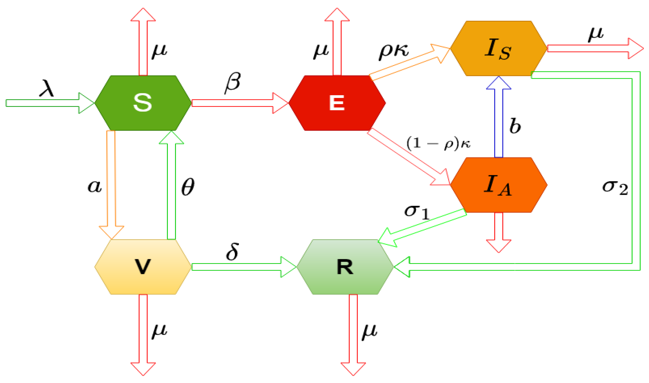
To capture the transmission dynamics of the Influenza virus, the total human population at any time t, denoted by , is stratified into six epidemiological compartments, each representing a distinct health status or disease progression phase:
(i) Susceptible population (): Individuals who have not yet contracted the virus and are at risk of infection through contact with infectious persons.
(ii) Exposed population (): Individuals who have been exposed to the virus and are in the incubation period. Although they do not show symptoms, they remain capable of transmitting the virus, thus contributing to its spread in the population.
(iii) Symptomatic infected population (): Individuals who have developed clinical symptoms of influenza and are actively contagious. This group represents the primary source of detectable and severe transmission cases.
(iv) Asymptomatic infected population (): Individuals who are infected but do not exhibit clinical symptoms. Despite their asymptomatic status, they play a critical role in the silent transmission of the virus.
(v) Recovered population (): Individuals who have overcome the infection and acquired immunity. They no longer participate in the transmission chain.
(vi) Vaccinated population (): Individuals who have received a vaccine and possess varying levels of protection depending on vaccine efficacy.
It is important to note that the exposed (), symptomatic infected (), and asymptomatic infected () compartments collectively represent the infected individuals, differentiated based on the presence or absence of clinical symptoms and the stage of infection. This stratification allows for a more nuanced depiction of viral transmission, particularly in accounting for asymptomatic carriers and pre-symptomatic transmission—a key challenge in managing influenza outbreaks.
To describe the progression and spread of influenza within the stratified population, and to incorporate the influence of media-driven public health interventions, we introduce the following deterministic system of nonlinear ordinary differential equations. This system models the time-dependent interactions among the compartments under the influence of media awareness, which can alter behavioral patterns such as adherence to preventive measures, rate of vaccination, or reduction in contact frequency with infected individuals.
with initial values
In the formulation of the epidemiological model described by equation (1), each parameter carries specific biological significance. These parameters, which collectively define the dynamics of population transitions under viral infection and vaccination strategies, are elucidated as follows:
- denotes the constant production rate of viral agents within the infected host population. This parameter captures the continual generation of infectious particles that contribute to disease propagation.
- represents the infection transmission rate, quantifying the probability of successful disease spread upon contact between susceptible and infectious individuals.
- The natural death rate of individuals within the model is denoted by , encompassing mortality unrelated to the disease or vaccination process.
- The parameter a characterizes the rate of vaccination administration across the population, effectively indicating the proportion of susceptible individuals receiving immunization over time.
- Vaccination efficacy is described by , which is assumed to be low; this reflects the limited protective effect conferred by the vaccine, potentially due to weak immune response or pathogen resistance. - The rate of progression from the exposed class to the infectious class is captured by , indicating the transition speed from latent infection to active disease.
- corresponds to the proportion of the population subject to disease transmission and progression, influencing the overall dynamics of the epidemic spread.
- The parameters and represent distinct recovery rates from infection, potentially differentiating recovery outcomes based on treatment status or disease severity.
- The recovery rate of vaccinated individuals who may still undergo infection is denoted by , incorporating post-vaccination outcomes within the model framework.
- The symbol b appears to be unassigned in the current context; clarification or specification is required to complete its interpretation.
The numerical values and descriptions of these parameters are comprehensively listed in Table 2, which supports the analytical and simulation aspects of the model.
Figure 1.
Diagrammatic representation of the model (1).
Figure 1.
Diagrammatic representation of the model (1).
3. Positive Invariance and Boundedness of Solutions
In order to analyze the behavior of the influenza virus, we present the following characteristics.
3.1. Positive Invariance
We have the following theorem on the nonnegative of solutions.
Theorem 1.
Proof.
Let
Using initial condition (2), we have . Also, are all equal to zero at if
From the first equation of (1), we can write
That is
Thus,
Hence,
So that,
Again, from system (1), we get
That is
Thus,
Hence,
So that,
Following the same procedure, we can show that for all, we get and . Thus, we conclude that all trajectories of system (1) remain positive in for any all . Hence, the proof is completed. □
3.2. Boundedness
We now begin with the theorem that guarantees that the solutions to system (1) are constrained to have nonnegative beginning values.
Theorem 2.
All solutions of system (1) are bounded in the region Ψ, defined by
4. Basic Reproduction Number, Equilibria and Stability Analysis
This section contains the derivation of basic reproduction number, existence of steady states and their stability analysis.
4.1. The Basic Reproduction Number
To calculate , we use next generation method [38]. We consider two vector and defined for the system (1).
Next, we are setting that the entry-wise non-negative new infection matrix is F, and G be the non-singular Metzler matrix [39] define the transitions of influenza infection between the infection compartments and the matrices, which are given as follows:
Therefore, we have,
With the help of Next generation matrix, we have the largest eigenvalue of at
4.2. Equilibrium Points
There are two equilibria of the system:
(i). The infection-free equilibrium is
(ii). The disease state equilibrium is where
and is the positive root of the following equation:
The calculation is complected. Thus we find a positive value of using numerical calculations.
4.3. Local Stability
Theorem 4.
The system is stable at when , and unstable when .
Proof.
At , we have,
Here the eigenvalues are and the other five eigenvalues are calculated from
and the characteristic equation for (7) is
where,
and where,
where,
For and . If , then roots must be negative. For , we get the threshold condition for . We get the condition which implies that which results the removal of infection. □
4.4. Local Equilibrium Stability of the Endemic System
Proof.
At , we have the charismatic equation
where,
At , the characteristic equation is
where,
Sum of the minor of order one along the main diagonal of
Sum of the minors of order two of the diagonal element of
Sum of the minors of order two of the diagonal element of, etc.
□
5. Parameter Sensitivity Analysis
Sensitivity and identifiability studies were conducted by computing the derivative of the clinical score with respect to the vector parameter at each data point. The sensitivities are dimensionless because of their scaling with respect to the values of the variables and parameters. The following is a representation of the system (1) sensitivity functions with respect to any parameter p:
Due to these sensitivities, the least important parameter for model output may be found and changed without being used for calibration. The sensitivity functions of DDEs can be found using a variety of techniques [18,40]. However, to determine the sensitivity functions of the system (1), we shall employ the so-called direct technique because of its simplicity.
According to the parameter , the relevant sensitivity system (1), given below
Similarly, the sensitivity of the other parameter can be studied.
6. Optimal Control Problem Formulation
In this section, we have considered two non-medical controls, like awareness through governance and self-learning, to control the disease. Here, our main focus is to minimize the number of infected and exposed people. For this purpose, we have introduced control strategies .
- Control represents the role of exposed class control.
- Control plays a crucial role in controlling the infected class.
Thus, our optimal control problem becomes
In the objection for is the cost induced by exposed clans, is the cost induced by the infected clam, is the cost induced by any phase infected class and on the cost induced by optimal stage, as the costs at stage.
Here the optimal controls where
where such that is Lebesgue measure on with }
6.1. Existence of an Optimal Control
Have we the existence of an optimal control model (12)
Theorem 5.
and exist for the stake initial value problem (12) and the (13) minimizes over
Proof.
For every admissible control , there is a unique solution satisfying the Lipsehiiz condition. Also, we know that the total population is bounded, and it belongs to . Also, all the state variables are bounded. Thus, we have a partial derivation of the state system (12) with respect to the state variable system bondedness, which satisfies condition . We can also verify condition by checking the liner dependence of the state equation and control , for verification function condition (iii). We note that linear and quarantine functions are convex [41]. To prove the bondedness on J, we have and an and .
To verify the existence condition, we use the study of family and Rishel’s theorem under certain conditions.
- Systems (12) and (13) with the control fraction V are non-empty.
- The state system should be a linear function dependent on time and time state variables.
- The integral J in (13) is convex on and the the exi and there exist a positive numbers and and such that
It follows,
from (14) we get
Thus,
where and . □
Theorem 6.
When , is globally asymptotically stable.
Proof.
Let be a Lyapunov function I in which we only consider the exposed and infected class. with positive contract . Then,
□
6.2. Characterization of the Optimal Control Pair
Let represent the amount of medicine as control input. The essential criteria for an optimum control and related states to meet Pontryagin’s Maximum Principle are represented by the cost function (13) for the system (12). We employ Pontryagin’s maximal principle [42] to choose the best controls for and . By using this technique, we create the Hamiltonian function L with regard to , which transforms the system (12) along with (13).
According to the control system provided by (12), we determine the problem’s optimal settings. To define the Lagrangian (), the Hamiltonian associated with the control problem generated in this way is also included.
The Hamiltonian is built as follows by combining the state variables and adjoint variables:
Here,
The adjoint system to be estimated for the control input associated with the model state variables is represented as For control input, along with is represented as
Here, the transversality conditions are Pontryagin’s Maximum Principle [42] has allowed us to ascertain
Then,
Solving(22) for and ,
The standard form is
Thus we can write as
Thus, the optimal system becomes
along with the transversality conditions: .
7. Numerical Simulations
In this section, we analyze our model and the optimal system graphically using Matlab simulations. All the parameters are taken from Table 2 and some parameters are varied for studying their impacts on the system dynamics.
As analysed in section 5, we plot the sensitivity of model parameters in Figure 2 and also in Table 3. All parameters are sensitive for the study of the H1N1 dynamics. Some parameters, namely etc., are positively sensitive and some parameters are negatively sensitive to the disease.
Figure 3 shows that when , the system attains its disease-free state. Also, when , the system moves to a stable endemic steady state. Figure 4 shows the forward bifurcation at the basic reproduction . We have varied the infection rate , and it is observed that when , the system becomes disease-free, and it shows its stability around . It switches to an endemic state when and the system attains stability around .
Figure 5 shows the stability region for the disease-free state and endemic state with respect to parameters and . From this figure, we reveal that with the increasing values of and , the system switches its stability from to that is from disease-free to endemic state. Nonlinear stability of the endemic system is shown in Figure 6. All phase trajectories converge to the same endemic steady state showing the global stability of .
Impact of is analyzing using the Figure 7 by plotting the equilibrium values of the model population with respect to . Similarly, in Figure 8, the impact of vaccination is shown. Infection is reduces as the vaccinated populations are increased.
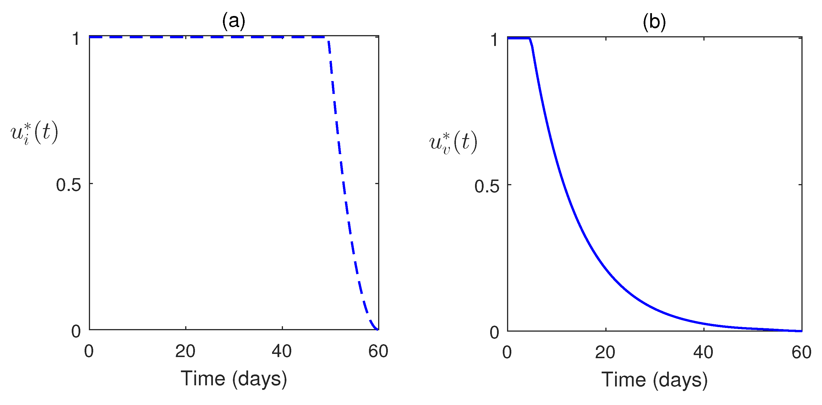
Also, we consider the control system with control inputs and for the systems (12) and (13). The time-dependent control functions, along with the state system and adjoint system, are analyzed numerically. Here, the optimal control problem is bounded by . Here, we consider at which the treatment is stopped. Optimal system is plotted in Figure 9. This figure shows the impacts of controls on the disease. In Figure 10, the optimal trajectories show the effective role of control strategies. Also, we have clearly observed that a low weight factor gives a better result in increasing the susceptible population along with class improvement.
8. Discussion and Conclusion
The H1N1 virus is a major contributor to influenza infections, primarily affecting the upper respiratory tract. Severe manifestations are typically observed in individuals with underlying chronic conditions. To better understand and mitigate the spread of this virus, a mathematical model has been developed and extended to incorporate time-dependent control inputs. The model framework includes the establishment of existence conditions and a thorough stability analysis based on the basic reproduction number, .
A comprehensive sensitivity analysis reveals that all model parameters significantly influence the dynamics of H1N1 transmission. Notably, parameters such as the transmission rate (), recruitment rate (), and contact rate () exhibit positive sensitivity, indicating that increases in these parameters tend to amplify the spread of infection (Figure 2).
We illustrated the critical role of the basic reproduction number in determining system behavior (Figure 3). When , the model stabilizes at a disease-free equilibrium (), whereas leads to a stable endemic equilibrium (). This transition is further substantiated by the forward bifurcation (Figure 4), which highlights a distinct shift in system dynamics as crosses the threshold value unity. We have seen that when endemic system is feasible, it is global stabile (Figure 6). The impact of the contact rate is examined which shows that higher values of correspond to increased equilibrium infection levels (Figure 7). This finding emphasizes the importance of managing contact rates to control disease spread. Additionally, the positive effect of vaccination is studied where an increase in vaccinated individuals leads to a marked reduction in infection prevalence (Figure 8).
For the analysis of the control model, Pontryagin’s Maximum Principle has been employed. The corresponding Hamiltonian function has been constructed, and the adjoint equations, along with the optimal control variables and , have been derived. To enhance disease mitigation, the model incorporates a control system governed by time-dependent inputs (vaccination) and (treatment), analyzed over a finite time horizon . We have seen that the optimal control strategies are effective. The simulations reveal that control interventions significantly reduce infection levels. Moreover, a lower weight factor in the cost function yields improved outcomes, including an increase in the susceptible population and enhanced class dynamics, suggesting that more aggressive control measures are beneficial (Figure 9 and Figure 10).
In summary, this study presents a rigorous analysis of the H1N1 transmission model, integrating sensitivity analysis, bifurcation theory, and optimal control strategies. The basic reproduction number serves as a pivotal threshold for system stability. Parameters such as , , and play critical roles in shaping disease dynamics. Vaccination and contact reduction are effective in curbing infection spread. Optimal control strategies, particularly those with lower cost weights, substantially improve population health outcomes.
In conclusion, the results underscore the importance of targeted interventions and strategic parameter management in controlling infectious diseases like H1N1. The integration of mathematical modeling and optimal control provides a valuable framework for public health decision-making and epidemic response planning.
Data Availability Statement
The data used for this study are mentioned within the article.
Acknowledgments
The authors extend their appreciation to the Deanship of Research and Graduate Studies at King Khalid University for funding this work through Large Group Project under grant number (58/ 46).
Conflicts of Interest
The authors declare no conflict of interest.
References
- Javanian, M.; Barary, M.; Ghebrehewet, S.; Koppolu, V.; Vasigala, V.; Ebrahimpour, S. A brief review of influenza virus infection. Journal of medical virology 2021, 93, 4638–4646. [Google Scholar] [CrossRef]
- Muthukutty, P.; MacDonald, J.; Yoo, S.Y. Combating Emerging Respiratory Viruses: Lessons and Future Antiviral Strategies. Vaccines 2024, 12, 1220. [Google Scholar] [CrossRef]
- Fallani, E. Public health impact of influenza vaccination in Italy: barriers, benefits and interventions in the field of prevention. 2023. [Google Scholar]
- Stephens, B.; Azimi, P.; Thoemmes, M.S.; Heidarinejad, M.; Allen, J.G.; Gilbert, J.A. Microbial exchange via fomites and implications for human health. Current Pollution Reports 2019, 5, 198–213. [Google Scholar] [CrossRef]
- Kakoullis, L.; Steffen, R.; Osterhaus, A.; Goeijenbier, M.; Rao, S.R.; Koiso, S.; Hyle, E.P.; Ryan, E.T.; LaRocque, R.C.; Chen, L.H. Influenza: seasonality and travel-related considerations. Journal of travel medicine 2023, 30, taad102. [Google Scholar] [CrossRef]
- Li, Y.; Wang, X.; Msosa, T.; de Wit, F.; Murdock, J.; Nair, H. The impact of the 2009 influenza pandemic on the seasonality of human respiratory syncytial virus: a systematic analysis. Influenza and other respiratory viruses 2021, 15, 804–812. [Google Scholar] [CrossRef] [PubMed]
- Germann, T.C.; Kadau, K.; Longini Jr, I.M.; Macken, C.A. Mitigation strategies for pandemic influenza in the United States. Proceedings of the National Academy of Sciences 2006, 103, 5935–5940. [Google Scholar] [CrossRef] [PubMed]
- Belshe, R.B.; Edwards, K.M.; Vesikari, T.; Black, S.V.; Walker, R.E.; Hultquist, M.; Kemble, G.; Connor, E.M. Live attenuated versus inactivated influenza vaccine in infants and young children. New England Journal of Medicine 2007, 356, 685–696. [Google Scholar] [CrossRef] [PubMed]
- Pawaiya, R.; Dhama, K.; Mahendran, M.; Tripathi, B. Swine flu and the current influenza A (H1N1) pandemic in humans: A review. Indian Journal of Veterinary Pathology 2009, 33, 1–17. [Google Scholar]
- Lo, J.Y.; Tsang, T.H.; Leung, Y.H.; Yeung, E.Y.; Wu, T.; Lim, W.W. Respiratory infections during SARS outbreak, Hong Kong, 2003. Emerging infectious diseases 2005, 11, 1738. [Google Scholar] [CrossRef]
- Zanobini, P.; Bonaccorsi, G.; Lorini, C.; Haag, M.; McGovern, I.; Paget, J.; Caini, S. Global patterns of seasonal influenza activity, duration of activity and virus (sub) type circulation from 2010 to 2020. Influenza and other respiratory viruses 2022, 16, 696–706. [Google Scholar] [CrossRef]
- Nypaver, C.; Dehlinger, C.; Carter, C. Influenza and influenza vaccine: a review. Journal of midwifery & women’s health 2021, 66, 45–53. [Google Scholar]
- Andre, F.E.; Booy, R.; Bock, H.L.; Clemens, J.; Datta, S.K.; John, T.J.; Lee, B.W.; Lolekha, S.; Peltola, H.; Ruff, T.; et al. Vaccination greatly reduces disease, disability, death and inequity worldwide. Bulletin of the World health organization 2008, 86, 140–146. [Google Scholar] [CrossRef]
- Ziegler, T.; Mamahit, A.; Cox, N.J. 65 years of influenza surveillance by a World Health Organization-coordinated global network. Influenza and other respiratory viruses 2018, 12, 558–565. [Google Scholar] [CrossRef] [PubMed]
- Ampofo, W.K.; Azziz-Baumgartner, E.; Bashir, U.; Cox, N.J.; Fasce, R.; Giovanni, M.; Grohmann, G.; Huang, S.; Katz, J.; Mironenko, A.; et al. Strengthening the influenza vaccine virus selection and development process: Report of the 3rd WHO Informal Consultation for Improving Influenza Vaccine Virus Selection held at WHO headquarters, Geneva, Switzerland, 1–3 April 2014. Vaccine 2015, 33, 4368–4382. [Google Scholar] [CrossRef] [PubMed]
- Tracht, S.M.; Del Valle, S.Y.; Hyman, J.M. Mathematical modeling of the effectiveness of facemasks in reducing the spread of novel influenza A (H1N1). PloS one 2010, 5, e9018. [Google Scholar] [CrossRef] [PubMed]
- Tchuenche, J.M.; Dube, N.; Bhunu, C.P.; Smith, R.J.; Bauch, C.T. The impact of media coverage on the transmission dynamics of human influenza. BMC public health 2011, 11, 1–14. [Google Scholar] [CrossRef]
- Krishnapriya, P.; Pitchaimani, M.; Witten, T.M. Mathematical analysis of an influenza A epidemic model with discrete delay. Journal of computational and Applied Mathematics 2017, 324, 155–172. [Google Scholar] [CrossRef]
- Kanyiri, C.W.; Mark, K.; Luboobi, L.; et al. Mathematical analysis of influenza A dynamics in the emergence of drug resistance. Computational and Mathematical Methods in Medicine 2018, 2018. [Google Scholar] [CrossRef]
- Kim, S.; Jung, E. Prioritization of vaccine strategy using an age-dependent mathematical model for 2009 A/H1N1 influenza in the Republic of Korea. Journal of Theoretical Biology 2019, 479, 97–105. [Google Scholar] [CrossRef]
- Dalal, A.; Gill, P.S.; Narang, J.; Prasad, M.; Mohan, H.; et al. Genosensor for rapid, sensitive, specific point-of-care detection of H1N1 influenza (swine flu). Process Biochemistry 2020, 98, 262–268. [Google Scholar]
- Ratre, Y.K.; Vishvakarma, N.K.; Bhaskar, L.; Verma, H.K. Dynamic propagation and impact of pandemic influenza A (2009 H1N1) in children: a detailed review. Current microbiology 2020, 77, 3809–3820. [Google Scholar] [CrossRef]
- Baba, I.A.; Ahmad, H.; Alsulami, M.; Abualnaja, K.M.; Altanji, M. A mathematical model to study resistance and non-resistance strains of influenza. Results in Physics 2021, 26, 104390. [Google Scholar] [CrossRef]
- Alharbi, M.H.; Kribs, C.M. A mathematical modeling study: assessing impact of mismatch between influenza vaccine strains and circulating strains in hajj. Bulletin of Mathematical Biology 2021, 83, 7. [Google Scholar] [CrossRef]
- Ackerman, E.E.; Weaver, J.J.; Shoemaker, J.E. Mathematical Modeling Finds Disparate Interferon Production Rates Drive Strain-Specific Immunodynamics during Deadly Influenza Infection. Viruses 2022, 14, 906. [Google Scholar] [CrossRef] [PubMed]
- Kamrujjaman, M.; Mohammad, K.M. Modeling H1N1 Influenza Transmission and Control: Epidemic Theory Insights Across Mexico, Italy, and South Africa. arXiv preprint 2024, arXiv:2412.00039. [Google Scholar]
- Mohammad, K.M.; Akhi, A.A.; Kamrujjaman, M. Bifurcation analysis of an influenza A (H1N1) model with treatment and vaccination. PloS one 2025, 20, e0315280. [Google Scholar] [CrossRef]
- Khan, A.; Waleed, M.; Imran, M. Mathematical analysis of an influenza epidemic model, formulation of different controlling strategies using optimal control and estimation of basic reproduction number. Mathematical and Computer Modelling of Dynamical Systems 2015, 21, 432–459. [Google Scholar] [CrossRef]
- Chebotaeva, V.; Srinivasan, A.; Vasquez, P.A. Differentiating Contact with Symptomatic and Asymptomatic Infectious Individuals in a SEIR Epidemic Model. Bulletin of Mathematical Biology 2025, 87, 38. [Google Scholar] [CrossRef]
- Srivastav, A.K.; Ghosh, M. Modeling and analysis of the symptomatic and asymptomatic infections of swine flu with optimal control. Modeling Earth Systems and Environment 2016, 2, 1–9. [Google Scholar] [CrossRef]
- Wu, J.; Dhingra, R.; Gambhir, M.; Remais, J.V. Sensitivity analysis of infectious disease models: methods, advances and their application. Journal of The Royal Society Interface 2013, 10, 20121018. [Google Scholar] [CrossRef]
- Arriola, L.; Hyman, J.M. Sensitivity analysis for uncertainty quantification in mathematical models. In Mathematical and statistical estimation approaches in epidemiology; Springer, 2009; pp. 195–247. [Google Scholar]
- Tchuenche, J.; Khamis, S.; Agusto, F.; Mpeshe, S. Optimal control and sensitivity analysis of an influenza model with treatment and vaccination. Acta biotheoretica 2011, 59, 1–28. [Google Scholar] [CrossRef]
- Lamwong, J.; Pongsumpun, P. Optimal control and stability analysis of influenza transmission dynamics with quarantine interventions. Modeling Earth Systems and Environment 2025, 11, 1–18. [Google Scholar] [CrossRef]
- Cheng, K.; Leung, P. What happened in China during the 1918 influenza pandemic? International Journal of Infectious Diseases 2007, 11, 360–364. [Google Scholar] [CrossRef] [PubMed]
- Saunders-Hastings, P.R.; Krewski, D. Reviewing the history of pandemic influenza: understanding patterns of emergence and transmission. Pathogens 2016, 5, 66. [Google Scholar] [CrossRef]
- e Souza, P.A.C.A.; Dias, C.M.; de Arruda, E.F. Optimal Control Model for Vaccination Against H1N1 Flu Modelo com Controle Ótimo para a Vacinação contra a Gripe H1N1. Ciências Exatas e Tecnológicas, Londrina 202, 41, 105–114. [Google Scholar] [CrossRef]
- Van den Driessche, P.; Watmough, J. Reproduction numbers and sub-threshold endemic equilibria for compartmental models of disease transmission. Mathematical biosciences 2002, 180, 29–48. [Google Scholar] [CrossRef] [PubMed]
- Narendra, K.S.; Shorten, R. Hurwitz Stability of Metzler Matrices. IEEE Transactions on Automatic Control 2010, 55, 1484–1487. [Google Scholar] [CrossRef]
- Rihan, F.A. Sensitivity analysis for dynamic systems with time-lags. Journal of Computational and Applied Mathematics 2003, 151, 445–462. [Google Scholar] [CrossRef]
- Fleming, W.H.; Rishel, R.W. Deterministic and stochastic optimal control; Springer Science & Business Media, 2012; Vol. 1. [Google Scholar]
- Pontryagin, L.S. Mathematical theory of optimal processes; CRC press, 1987. [Google Scholar]
Figure 2.
Sensitivity of the model parameters with respect to the
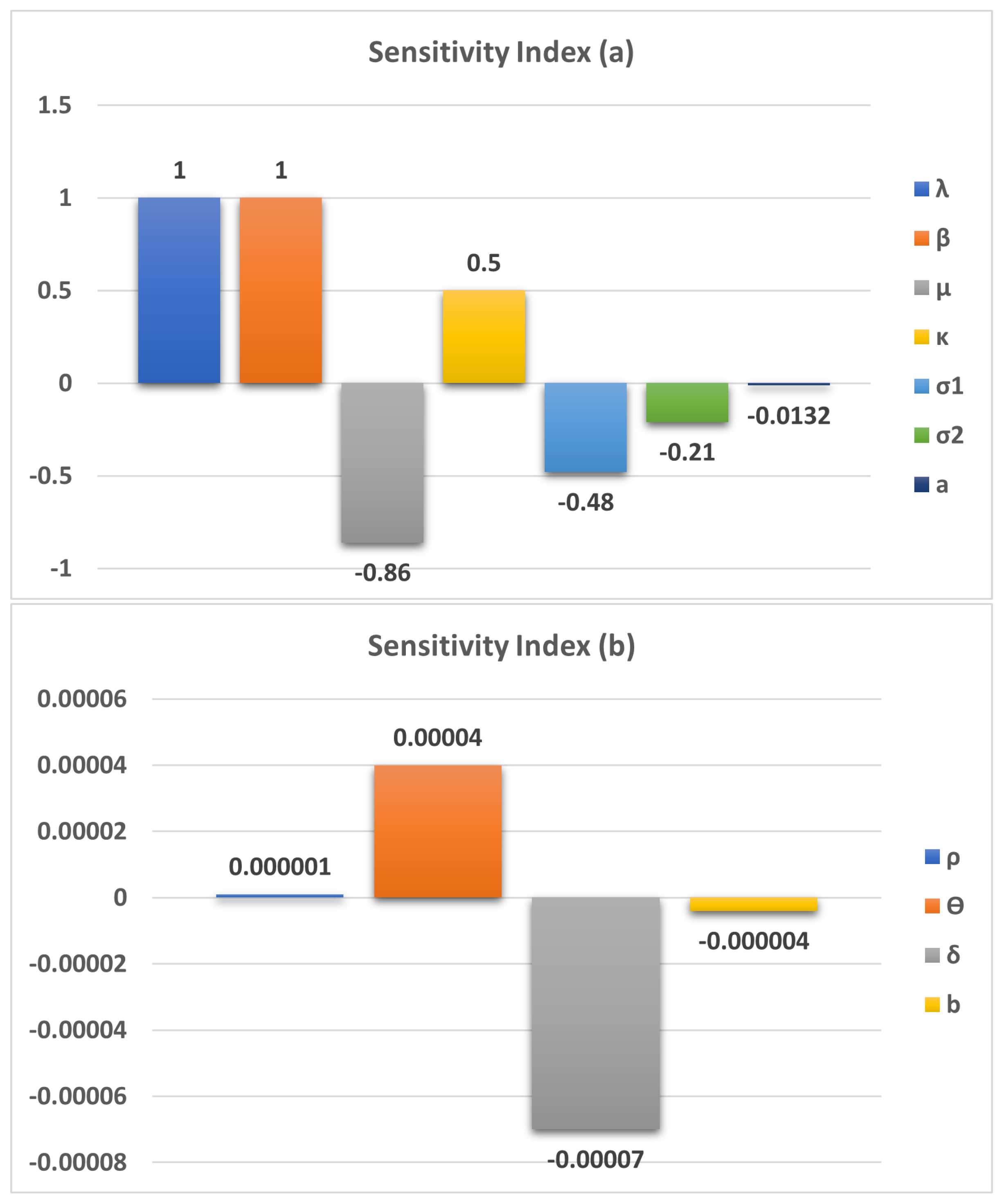
Figure 3.
Simulation of model variables when . Parameter values are taken from Table 2.
Figure 3.
Simulation of model variables when . Parameter values are taken from Table 2.
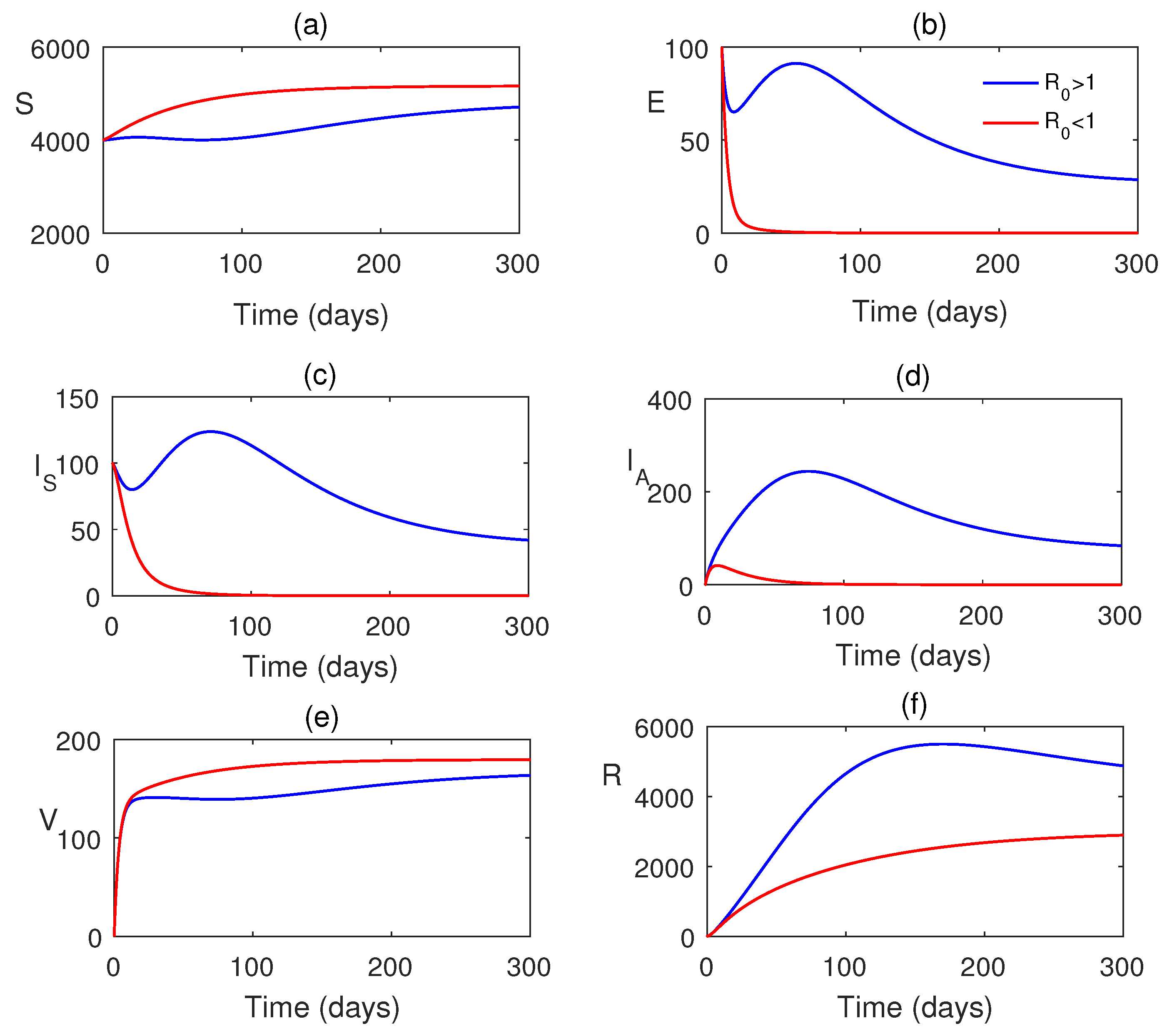
Figure 4.
Forward bifurcation plot showing the steady stable values of exposed, symptomatic infected population, and asymptomatic infected population with respect to . Except parameter , the parameter values are kept same as in Table 2.
Figure 4.
Forward bifurcation plot showing the steady stable values of exposed, symptomatic infected population, and asymptomatic infected population with respect to . Except parameter , the parameter values are kept same as in Table 2.
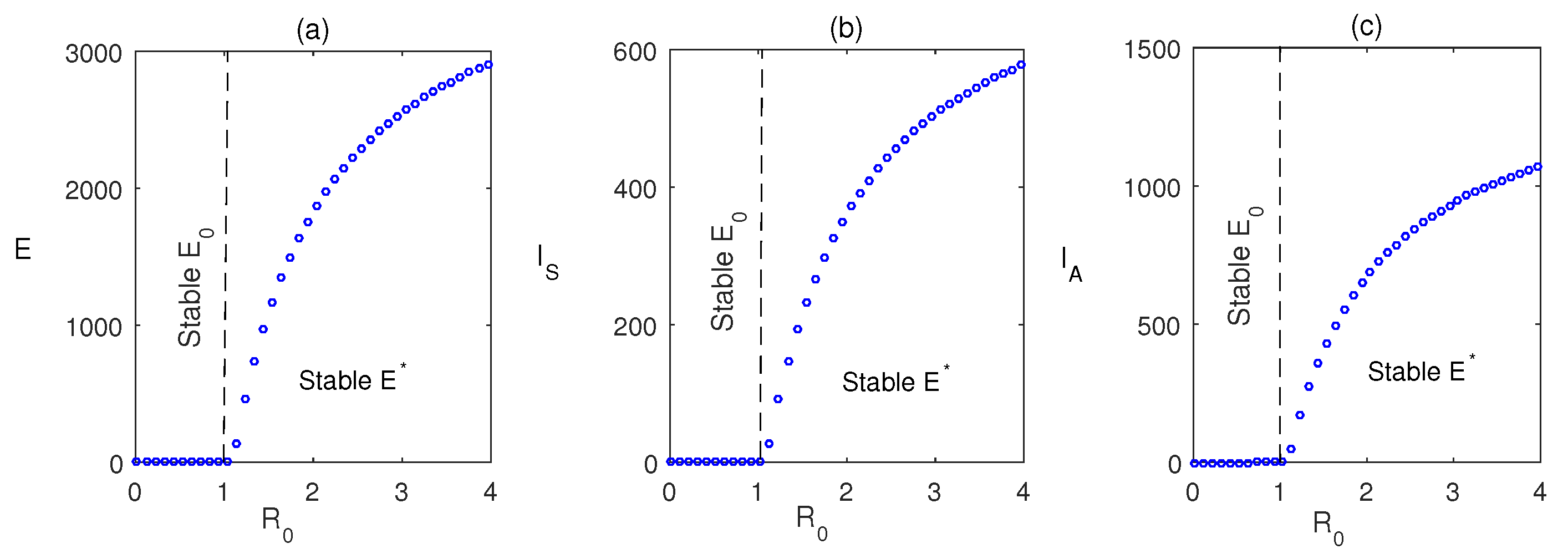
Figure 5.
Region of stability of disease-free equilibrium in: (a) , (b) parameter planes. Colour code denotes the value of .
Figure 5.
Region of stability of disease-free equilibrium in: (a) , (b) parameter planes. Colour code denotes the value of .
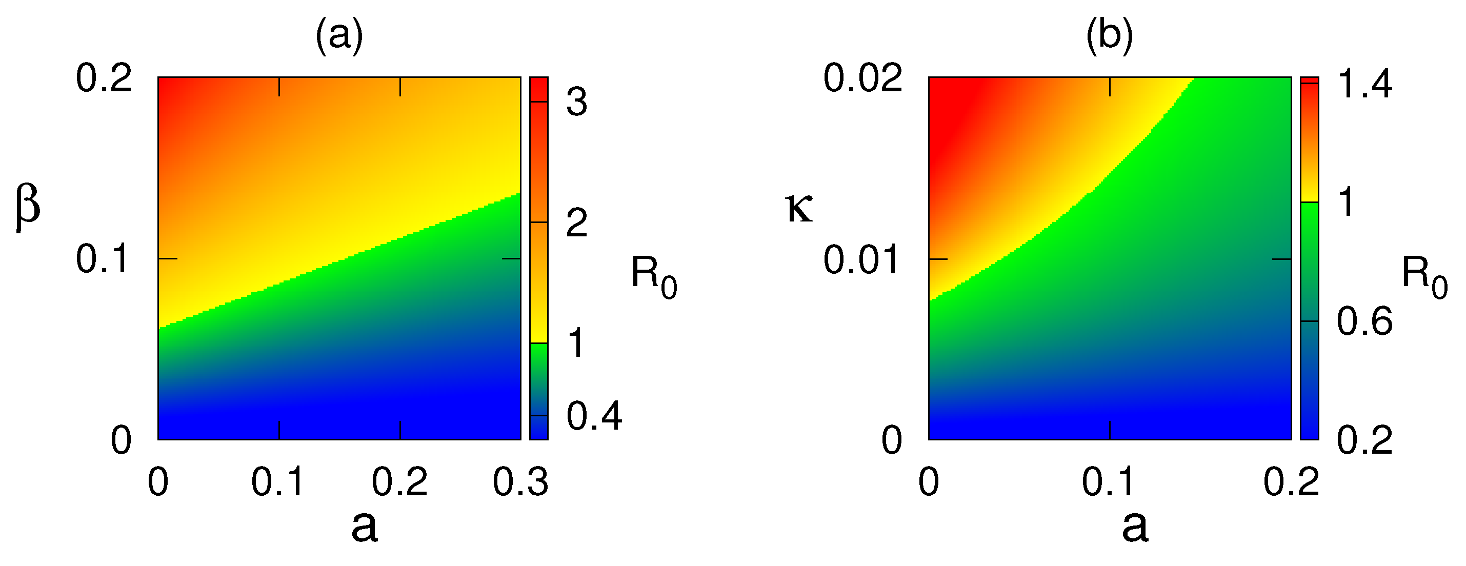
Figure 6.
Nonlinear stability: Phase trajectories are plotted when for three different initial values.
Figure 6.
Nonlinear stability: Phase trajectories are plotted when for three different initial values.
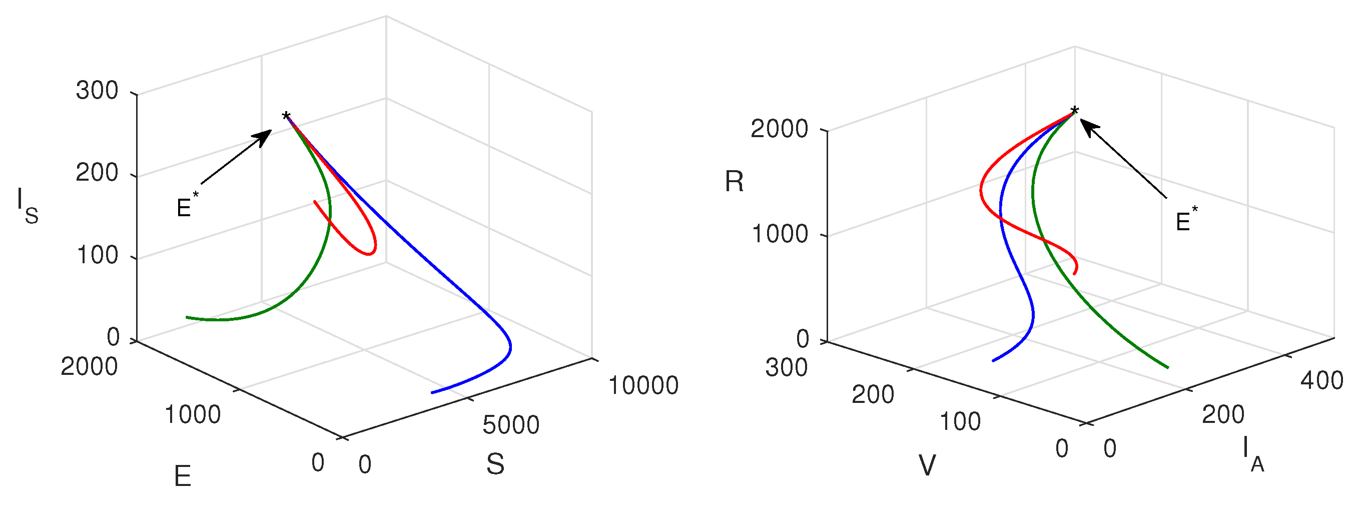
Figure 7.
Equilibrium values of the model populations plotted with respect to parameter . Other values of the parameters are same as given in Table 2.
Figure 7.
Equilibrium values of the model populations plotted with respect to parameter . Other values of the parameters are same as given in Table 2.
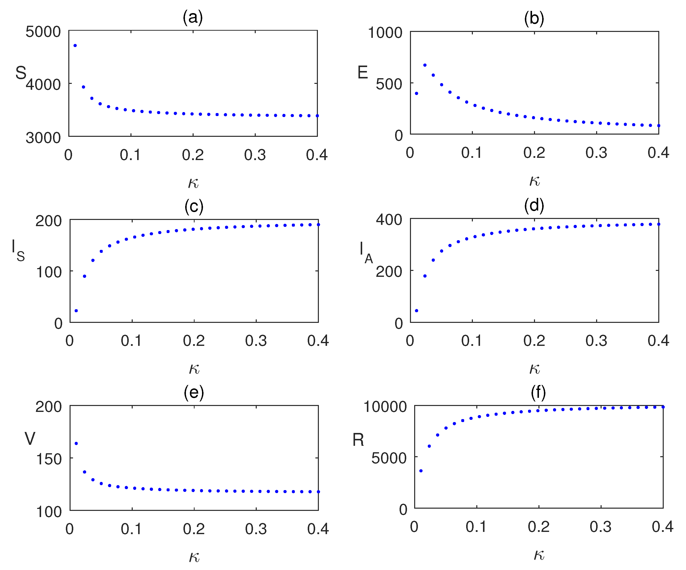
Figure 8.
Equilibrium values of the model populations plotted with respect to parameter a. Other values of the parameters are same as in Figure 7.
Figure 8.
Equilibrium values of the model populations plotted with respect to parameter a. Other values of the parameters are same as in Figure 7.
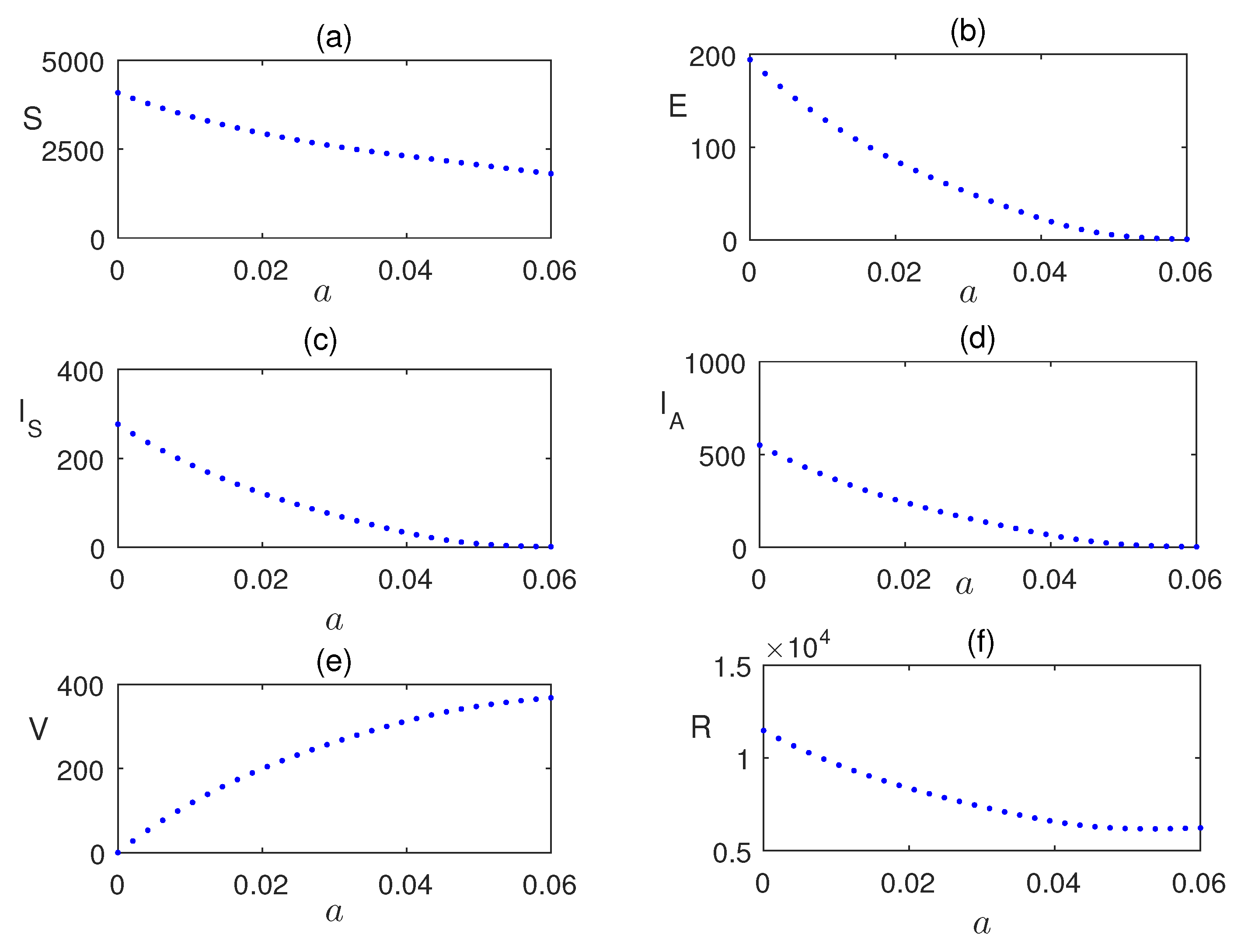
Figure 9.
Model simulation in presence of optimal control input for and Rest of the parameters are taken from Table 2.
Figure 9.
Model simulation in presence of optimal control input for and Rest of the parameters are taken from Table 2.
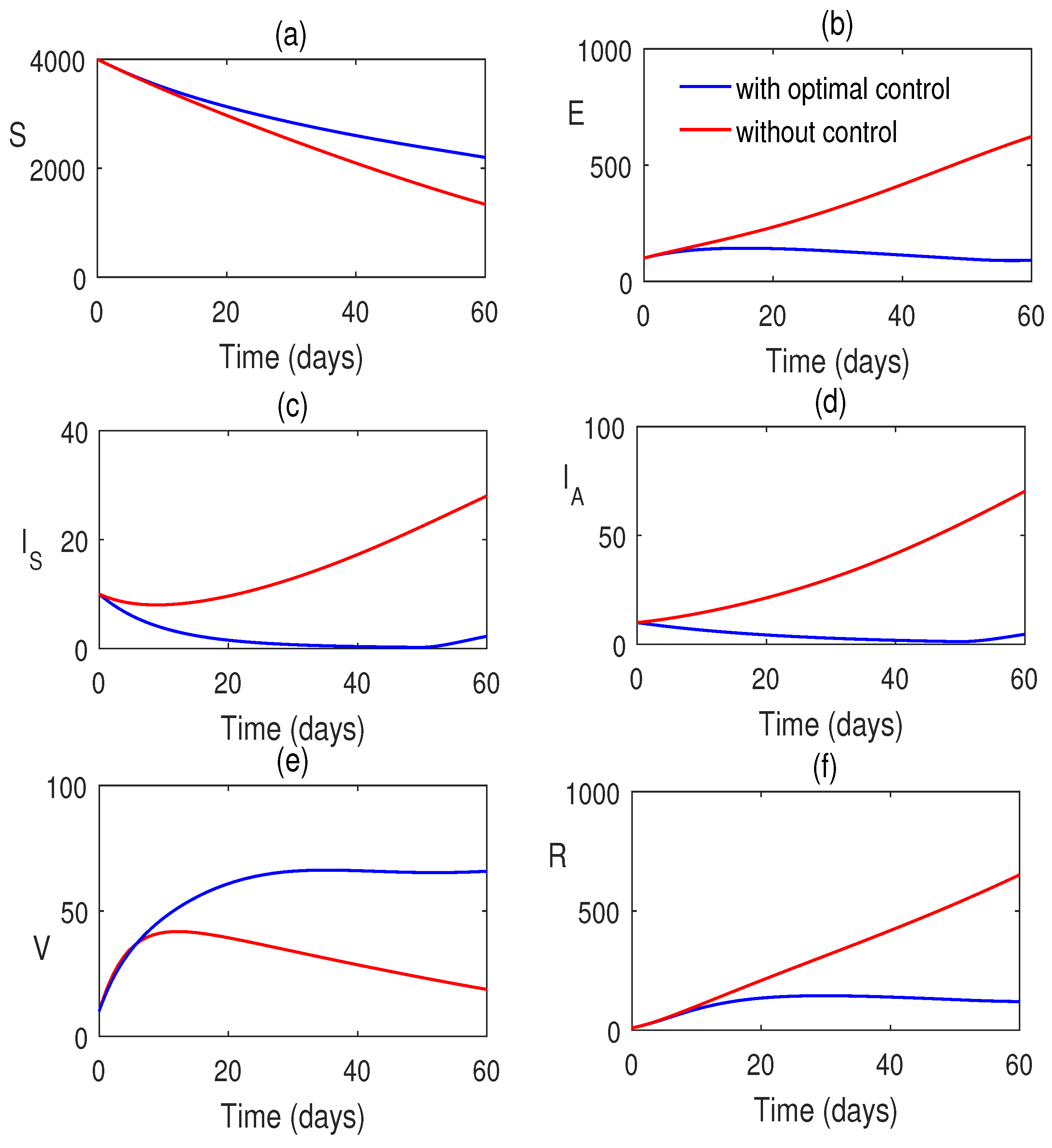
Figure 10.
Optimal control pair is plotted for parameter values as in Figure 9.
Figure 10.
Optimal control pair is plotted for parameter values as in Figure 9.
| Parameter | Definition | Value |
|---|---|---|
| Constant reproduction rate | ||
| Disease transmission rate | ||
| Death rate | 0.2 | |
| Rate of loss of immunity | 0.00833 | |
| a | Rate of vaccination | 0.0027375 |
| Rate of infraction from exposed population | ||
| Probability of population | ||
| 0.2 | ||
| and | The rate of recovery for the affected population | |
| b | 0.0027 | |
| Rate at which the vaccination recovers |
Table 3.
Sensitivity index of the parameters are presented.
| Parameter | a | ||||||
|---|---|---|---|---|---|---|---|
| Sensitivity Index | 1 | 1 | -0.86 | 0.5 | -0.48 | -0.21 | -0.0132 |
| Parameter | b | ||||||
| Sensitivity Index | 0.000001 | 0.00004 | -0.00007 | -0.000004 |
Disclaimer/Publisher’s Note: The statements, opinions and data contained in all publications are solely those of the individual author(s) and contributor(s) and not of MDPI and/or the editor(s). MDPI and/or the editor(s) disclaim responsibility for any injury to people or property resulting from any ideas, methods, instructions or products referred to in the content. |
© 2025 by the authors. Licensee MDPI, Basel, Switzerland. This article is an open access article distributed under the terms and conditions of the Creative Commons Attribution (CC BY) license (http://creativecommons.org/licenses/by/4.0/).
Copyright: This open access article is published under a Creative Commons CC BY 4.0 license, which permit the free download, distribution, and reuse, provided that the author and preprint are cited in any reuse.


