
Submitted:
15 August 2025
Posted:
19 August 2025
You are already at the latest version
Abstract
Pipeline systems are essential across various industries for transporting fluids over various ranges of distances. A notable application is natural circulation through thermo-syphoning, driven by temperature-induced density variations that generate fluid flow in closed loops. This passive mechanism is widely employed in sectors such as process engineering, oil and gas, geothermal energy, solar water heaters and fertilizers etc. Natural circulation loops eliminate the need for mechanical pumps, reducing both energy consumption and maintenance costs. This study investigates thermo-syphoning in a rectangular closed-loop system and develops an optimal control strategies like Linear Quadratic Control (LQR) and Model Predictive Control (MPC) to ensure stable and efficient heat removal while explicitly addressing physical constraints. The results demonstrate that MPC improves system stability and reduces energy usage through optimized control actions. Compared to the LQR and unconstrained MPC, MPC with active constraints effectively manages input limitations, ensuring safer and more practical operation. With its predictive capability and adaptability, the proposed MPC framework offers a robust, scalable solution for real-time industrial applications, supporting the development of sustainable and adaptive natural circulation pipeline systems.
Keywords:
Model Predictive Control
; Linear Quadratic Control
; Natural Circulation
; Thermo-syphoning
; Pipeline systems
1. Introduction
Pipelines are basically a network of interconnected pipes linked with pumps, control valves, instruments etc. that are used to transport the fluids from one point of location to another location [1]. The pipeline systems are integral to various industries as they enable the transportation of fluids over long distances. There are various applications of these pipelines as these are abundantly used in chemical industries, geothermal systems, solar water heating systems, oil and gas sector, water distribution, wastewater management, power generation and many more.
Various geometries and conditions were employed in such investigations, each possessing its own significance. Literature pertaining to these issues can be categorized based on the geometries and investigation methods utilized. Regarding geometry classification, it may involve either an open-loop or closed-loop configuration. Different methods for conducting these studies can be characterized into various numerical techniques, diverse analytic approaches, and various experimental methods.
This particular section encompasses the literature review on these three items, (a) Effect of using various configurations for natural circulation,(b) Effect of varying boundary and operating conditions,(c) Process dynamics and control of thermo-syphoning loops.
Natural circulation or thermo-syphoning loops are broadly categorized into two main types: single-phase thermo-syphoning loops and two-phase thermo-syphoning loops. This literature review primarily focuses on single-phase natural circulation in thermo-syphoning loops, where heat is transferred from a heat source to a heat sink. The orientation of the thermo-syphoning loop significantly influences its performance [2]. Schematic representations of some of these loops are provided in Figure 1 [3] .
In Figure 1 (a), a typical vertical loop is depicted, comprising a heat source and a heat sink. Heat moves from the source to the sink due to density or buoyancy gradients. Figure 1 (b) illustrates toroidal loops, where constant heat flux is typically applied to the bottom half while the upper half maintains a constant wall temperature boundary condition. Once again, heat transfer occurs through natural circulation driven by density or buoyancy gradients. Figure 1(c) demonstrates parallel branches with various heat or cooling fluxes of different magnitudes, facilitating the natural circulation phenomenon. Figure 1(d) displays an open square loop with heating coils at the bottom and two cooling coils open-ended at the top. Cold water flows from cold storage tanks under gravity, passing through heating coils, and warm water flows in the same legs towards cold storage tanks. In Figure 1(e), a closed square loop is shown, featuring a heating section at the bottom and a cooling section at the top.
However, the performance of rectangular closed loop was compared with toroidal loop by Basu et al. [4] and it was concluded that rectangular loops induce larger fluid flows than the toroidal loops undergoing identical dimensions, operating and boundary conditions, however, the stability span for toroidal geometry was found wider as compared to rectangular geometry.
Fichera et al. [5] compared the dynamics of two rectangular loops having different tube diameters and lengths, reported the important results that the loop having smaller diameter demonstrate more periodic behavior as compared to the loop having larger dimensions whose behavior is relatively more chaotic.
The effect of varying thermal boundary condition was studied by misale et al. [6], and it was inferred that varying the heat sink temperature could lead to crossing the stability threshold, highlighting the significance of this thermal boundary condition in influencing the system’s dynamics. In another study [7], it was noticed that as heater power increases, there’s a notable shift in the dynamics of fluid flow within the loop. Initially, loop characteristics remain stable up to a specific heater power level. However, beyond this threshold, the system transitions from steady behavior to periodic oscillations, and eventually to chaotic patterns.
The dynamics of rectangular closed loop was compared by subjecting it to different types of input powers such as step, ramp, and exponential profiles [8]. Exponential signals in modified form outperforms others in terms of stability both during increasing and decreasing power levels. Hashemi-Tilehnoee et al. [9] highlighted the role of natural circulation loops in passive heat transfer across diverse applications, emphasizing advances in working fluids, configurations, and modeling techniques to improve efficiency, stability, and safety in next-generation thermal systems.
A neural network–based NARMAX model [10] was developed to capture the unstable dynamics of a closed-loop thermosyphon from experimental input–output data, showing much closer agreement with measurements than an existing mathematical model. However, experimental and theoretical studies on thermal convection loops have shown that optimal and adaptive controllers can effectively suppress chaotic convection, outperforming neural network controllers in stability and efficiency, though the latter offer advantages in handling unknown nominal conditions and time delays [11].
Muscato et al. [12] derives a low-order non-linear model aligned with experimental observations, validated through simulation-experiment comparisons. It was observed that the dynamics of the natural circulation becomes unstable on higher heat fluxes, however at lower heat fluxes, the flow in the rectangular loop is not so efficient in terms of heat exchange in the cooling section. This model facilitated controller design for fluid motion stabilization, ensuring effective heat dissipation. Both conventional proportional and proportional-derivative controllers, considering the fluid velocity or temperature difference as feedback, were designed for various heating powers. Simulation results demonstrated confirmed the controllers’ effectiveness in stabilizing the system at desired equilibrium points.
A. Fichera et al. [13] developed a finite-order model of rectangular natural circulation loops by reducing a Fourier-series-based formulation of the momentum and energy equations to seven equations capturing the first three dynamic modes. Compared with Muscato et al.’s lower-order lumped-parameter model, which targeted specific nominal equilibrium points, Fichera’s higher-fidelity approach reproduced complex oscillatory behavior more accurately and supported controller design for a broader range of unstable dynamics.
Cammarata et al. [14] implemented an optimal control in the rectangular configuration and reported that the adopted strategy for the optimal controller is quite capable to minimizes a functional considering both system stability and control cost, weighted appropriately. Simulations and experimental implementation confirmed the effectiveness of the optimal controller in suppressing the hazardous oscillations and flow reversals, guiding the system to the desired steady state.
In geothermal pipeline or solar water heating systems based on Natural Circulation Loops (NCLs), where the primary objective is to extract maximum heat with a cooling water, stable and efficient operation is fundamental to ensuring long-term sustainability of energy extraction. Due to their reliance on buoyancy-driven flow without mechanical pumping, NCLs are inherently sensitive to variations in thermal and hydraulic conditions, making them vulnerable to instabilities, oscillations, and thermal stresses. While advanced control methods have been investigated for various renewable energy systems, the application of Model Predictive Control (MPC) to NCL-driven geothermal pipelines has not, to the best of our knowledge, been reported in the literature. This study addresses this research gap by introducing a predictive, optimization-based control strategy that utilizes an NCL dynamic model to forecast system responses and implement optimal control actions. The proposed approach enhances thermal stability, mitigates flow oscillations to prevent the excessive material stresses, thereby supporting both operational efficiency and the sustainable exploitation of geothermal or solar resources.
A key strength of the proposed MPC framework lies in its ability to explicitly incorporate operational and physical constraints into the control optimization problem. These constraints include maximum allowable temperatures and pressures to preserve material integrity, flow rate limits to minimize erosion and scaling, and bounds on heat extraction rates to prevent reservoir over-exploitation. Unlike conventional control methods, MPC ensures that these safety and sustainability criteria are respected at all times, even under variable operating conditions. By integrating predictive control with constraint handling, this work offers a novel pathway to improve process reliability to extend infrastructure lifespan, and enhance the environmental compatibility of geothermal energy systems. In this particular study, the test assembly consists of a rectangular loop with a heating section in the bottom horizontal leg and a cooling section in the top horizontal leg, connected by adiabatic vertical riser and downcomer tubes. The primary objective is to develop an MPC framework capable of achieving effective and stable heat removal by regulating the cooling rate, while explicitly incorporating physical constraints such as maximum and minimum coolant flow capacity. By leveraging MPC’s predictive capabilities, the proposed approach aims to enhance system stability, improve operational safety, and optimize equipment sizing, ultimately contributing to energy efficiency, reduced maintenance requirements, and the broader adoption of sustainable passive thermal management technologies in industrial applications.
2. Configuration of Experimental Setup
The Figure 2 illustrates the experimental arrangement for a single-phase natural circulation system [12]. This setup primarily comprises heating and cooling sections positioned in the lower and upper horizontal parts of the loop, respectively, interconnected via adiabatic vertical glass tubes. The heating section utilizes a variable heater with adjustable heating power, while the cooling section incorporates a double-pipe heat exchanger. Here, the main water flow passes through the inner copper tube, while tap water is injected into the annular pipe to extract heat from the inner fluid. The flow rate of the tap water is regulated by a controller.
The dimensions of the entire experimental setup are outlined in Table 1.
3. Mathematical Modeling for Natural Circulation Loop (NCL)
The assumptions that have been made for the natural circulation model are;(i) The bulk fluid flow is only in axial direction, (ii) The system behaves iso-thermally in the entire loop except heating and cooling sections. Therefore, the heat supplied by the heating section will be extracted in the cooling section, (iii) The cross-sectional area of loop remains constant throughout the axial direction, (iv) The fluid in the loop remains single phase during the entire operation. The mathematical model for natural circulation based on the fundamental conservation laws of momentum and energy can be described [12] as follows.
Where and denote the spatial and temporal domains respectively. Here, T, v, , D, g, , , and represent the fluid temperature in the loop, fluid velocity, thermal diffusivity, inner tube diameter, gravitational acceleration, volumetric expansion coefficient, reference temperature, and initial velocity, respectively.
The functions and depend on the geometry of the rectangular closed-loop system and are given as:
where and and in Equation (5) can be defined as follows;
Where q is the heat flux, is the temperature gradient between the entrance and exit of the cooling section, m is the mass flow rate, and is the heat capacity of the cooling water.
A key physical assumption that ensures the presence of equilibrium points is that the total heat energy transferred to the fluid as it passes through the heat source is exactly balanced by the heat energy removed as it flows through the heat sink. Based on this principle, we have:
which in turn implies:
The main model equations (1) and (2) can be further simplified by introducing Fourier Series expansion [15] of state variables T as follows:
Here, is a complex number. From equation (5) and geometrical considerations, where (i.e., the set of all nonzero integers), substituting expressions (9)–(11) into (1) and (2) yields the following system of infinite ordinary differential equations:
where , , and . Note that modes not in K decay, while modes in K but not in J are dependent variables.
In the case of the rectangular loops considered here, the coefficients from the expansion of are obtained from the following expression:
For simplification, we introduce the following substitutions:
With the substitutions applied and considering the specific form of , the coefficients for the rectangular geometry simplify to:
The coefficients vanish when k is even. As a result, the set J consists only of odd integers. Furthermore, some coefficients may also vanish for odd k if the circuit’s aspect ratio is rational.
In a similar fashion, the coefficients arising from the expansion of can be computed using:
By again applying substitution (15) and introducing the following definitions:
the expressions for in the considered case are obtained as:
Notably, since from the earlier result , this leads to the conclusion that all even-mode coefficients vanish. Therefore, the set K again consists solely of odd integers.
Now, after plugging eqs. (10)–(12) into the main model equations (1) and (2), and subsequently calculating the respective coefficients, truncating the Fourier Series expansion at its third mode (k=3) and applying the method of residuals for the separation of the real and imaginary parts of same order [12], we might be able to get the following seven ODEs to represent the overall system:
where,
According to our second assumption mentioned earlier in this section, the existence of equilibrium point is ensured. Usually, the first step after formulating the model equations, is to find the equilibrium points followed by linearization of the system around these equilibrium points. The properties that are considered for this study are presented in Table 2.
The Jacobian matrix of the system is a square matrix, with each element being the partial derivative of the equation with respect to the variable.
Similarly, the matrix was calculated as follows:
So, the linearized system in continuous time settings can be written as:
The above system can be discretized using suitable time step, and represented as follows;
The controllability matrix is similarly defined as:
Controllability Condition
The system is said to be controllable if and only if[16]:
where n is the dimension of the state vector x; here in our settings, the system was not found fully controllable, as the rank of the controllability matrix was 5. However, for such systems which are not fully controllable, it is advised to check the stabilizability. From PBH test (procedure details can be seen in Appendix A.1), it was found that all the uncontrolled eigenvalues are stable. The details of eigenvalues through controllability and stability analysis are shown in the following Figure 3. Three of the eigenvalues (green) are stable and controllable, two (pink) are unstable but controllable and rest of the two eigenvalues (blue) are uncontrollable but stable.
4. Discrete-Time Linear Quadratic Regulator (dLQR)
To develop an optimal control strategy for the discrete system, a discrete-time Linear Quadratic Regulator (dLQR) was designed. The discrete-time linearized model, characterized by the state-space matrices and were used for the controller design.
The performance index for the dLQR is defined as:
Here, Q and R, the weighting matrices are used to penalize state deviations and control effort respectively. In this work, they were selected as:
The dLQR gain is obtained by solving the Discrete-Time Algebraic Riccati Equation (DARE) [17]:
The matrix P can be computed using the "dare" command in MATLAB. The optimal state-feedback gain matrix K is then given by:
The corresponding optimal control input is:
When this control law is applied to the discrete-time state-space model, the closed-loop dynamics become:
Once the model states have been calculated, the final step will be the reconstruction of temperature function from these model states i.e. and using the following equation.
5. Linear Model Predictive Control (LMPC)
To extend the optimal control framework for this multivariable system, a Linear Model Predictive Control (LMPC) strategy was implemented. MPC is particularly useful for multiple-input multiple-output (MIMO) systems and for directly handling system constraints [18]. These features make MPC a natural choice for this case study.
5.1. Discrete-Time Linear Model
The continuous-time nonlinear dynamics were linearized and discretized with a sampling time of s, producing the discrete-time state-space model:
5.2. MPC Cost Function with Terminal Penalty
The finite-horizon quadratic cost function is defined as:
Here: penalizes state deviations, penalizes control effort and P is the terminal cost matrix obtained from the Discrete Algebraic Riccati Equation (DARE) for the unconstrained infinite-horizon LQR problem. This choice of P guarantees closed-loop stability when constraints are inactive.
5.3. Prediction Model for Quadratic Programming (QP) Formulation
For LMPC framework, built-in program "quadprog" of MATLAB was used [19]. However, lets define the stacked control sequence and the predicted states over the horizon (N) as::
The states can be expressed in terms of the initial condition and as:
where:
5.4. Quadratic Program (QP) Matrices H and f
The cost function can be rewritten as [19,20] :
where the Hessian matrix H and the linear cost vector are given by
Here, and define the stacked state prediction model, and , are block-diagonal matrices formed from , and terminal cost P.
where:
and:
Here, and are the stacked state and input setpoints over the horizon. The details of derivation of Quadratic Cost Function for MPC can be found in Appendix A.2.
5.5. Constraints
In this study, only input constraints were considered:
These are converted to a compact inequality constraint:
where G and are constructed to represent the bounds for each input over the prediction horizon.
6. Results
This section will be used to display results obtained from the discrete Linear Quadratic Control (dLQR) and Linear Model Predictive Control (LMPC) with and without constraints implemented on the natural circulation pipeline system.
The estimated states and control input, represented as deviation variables, obtained using LQR, unconstrained MPC, and constrained linear MPC are illustrated in Figure 4. The dLQR and unconstrained MPC yield identical responses. However, due to the imposed input constraints (Umin = -0.784 and Umax = 1.518), the constrained MPC exhibits an initial overshoot in the temperature state. Despite this, the system reaches steady state within 65 seconds, and the overall response remains smooth and free from oscillations. from Equation (18) used as control input obtained all the controllers was also plotted in Figure 4.
6.1. Remarks on dLQR vs. MPC
When the constraints are inactive, the optimal solution from Linear MPC coincides with the discrete-time LQR (dLQR) control law [21]:
where K is obtained from DARE. The primary advantage of LMPC is realized when constraints become active, as the optimizer adjusts future inputs to satisfy them while minimizing the cost, enabling safe and feasible operation under system limits.
The performance of MPC is highly sensitive to initial conditions, with greater deviations from the steady state requiring correspondingly higher control effort. This effect was examined by initiating control after different durations of open-loop operation. Due to the inherent instability of the system, longer delays resulted in the system state moving further from the steady state, thereby increasing the control effort demanded from the controller. The resulting comparison is presented in Figure 5. As a result, physical constraints be violated by conventional LQR or unconstrained MPC, and constrained MPC is very useful tool in considering such constraints.
used as control input, which consists of both coolant flow rate and the power heater. Here in our case, it was assumed that power of the heating in the heating section will remain fixed and coolant flow rate will be manipulated as control input. Such applications with fixed available heat source can be found in geothermal systems. Here, in our case, the estimated flow rate of the coolant as "control input" with fixed heater power (Q) =1800 W is shown in the Figure 5.
In this example, the primary physical constraint is the maximum flow capacity of the coolant pump. As shown in Figure 5, when the initial conditions deviate further from the steady state, the controller must exert greater control effort to stabilize the system. This increased demand can lead to the physical constraint being reached or exceeded, effectively surpassing the pump’s maximum flow capacity. Consequently, a pump with a higher capacity may be required to meet the control objectives under such conditions. One of the significant advantages of employing constrained MPC is that it enables the proper selection of pump capacity, ensuring maximum heat removal from the natural circulation loop while respecting system limitations. Moreover, by explicitly accounting for such constraints during controller design, MPC can prevent operational violations, improve system safety, and optimize equipment sizing for both performance and cost-effectiveness.
7. Discussion
Pipeline systems are fundamental to a wide range of industrial operations, and ensuring their reliability is essential for maintaining both safety and efficiency. Among these systems, natural circulation loops present distinct challenges due to their dependence on buoyancy-driven flow rather than mechanical pumping. This inherent characteristic makes them particularly susceptible to disturbances, where flow instabilities can significantly impact both performance and operational safety.
This study investigates the use of Model Predictive Control (MPC) as an effective approach for removal of heat in natural circulation pipelines used in geothermal systems. Findings show that MPC not only stabilizes system dynamics but also optimizes control efforts, which are closely tied to heating or cooling costs. When compared with conventional methods such as the Linear Quadratic Regulator (LQR), MPC gives an advantage of setting physical constraints on control action.
One of MPC’s key advantages is its capacity to manage input constraints explicitly. This allows for more practical and safer control actions that respect the physical and operational boundaries of system components like valves, actuators, sensors , maximum voltage capacity of the motor/pump, which may exhibit nonlinear behaviors or operational limits. Furthermore, MPC’s predictive capabilities enable it to respond proactively to dynamic conditions such as process fluctuations, thermal feedback, and variable flow rates.
From an implementation perspective, the control framework proposed in this research emphasizes both computational efficiency and ease of deployment, making it well-suited for industrial applications. By utilizing scalable control logic and adaptable system models, the approach effectively translates theoretical control concepts into practical, field-ready solutions.
In conclusion, incorporating MPC into natural circulation pipeline systems represents a promising strategy for improving process reliability and operational safety. Beyond its role as a control method, MPC has the potential to serve as a core component of advanced pipeline management systems.
Author Contributions
Conceptualization, A.H. and S.D.; methodology, A.H., G.O.C and S.D.; software, A.H.; validation, A.H., G.O.C; investigation, A.H. and S.A.B.; resources, S.D.; data curation, A.H.; writing—original draft preparation, A.H.; writing—review and editing, A.H. S.D.; visualization, A.H., G.O.C and S.D.; supervision, S.D.; project administration, G.O.C and S.D.; funding acquisition, N.A. All authors have read and agreed to the published version of the manuscript.
Funding
This research received no external funding.
Data Availability Statement
The data presented in this study are available on request from the corresponding author.
Acknowledgments
We want to acknowledge the support of University of Alberta. First author has acknowledged the scholarship achieved from "Higher Education Commission (HEC), Pakistan" and "Pipeline Simulation Interest Group (PSIG)"for the pursuit of his doctoral studies at University of Alberta”
Conflicts of Interest
The authors declare no conflicts of interest.
Abbreviations
The following abbreviations are used in this manuscript:
| CT | Continuous Time |
| LQR | Linear Quadratic Control |
| MIMO | Multi Input Multi Outputs |
| MPC | Model Predictive Control |
| ID | Inner Diameter |
Appendix A
Appendix A.1. Details of PBH Test for stabilizability [13]
Consider the discrete-time linear system:
where , .
- Compute the eigenvalues of the system matrix : denote them as .
- For each eigenvalue such that , verify controllability using the Popov–Belevitch–Hautus (PBH) test:where n is the number of states in the system.
- If the PBH test is satisfied for all unstable (or marginally unstable) eigenvalues, then the system is said to be stabilizable.
Appendix A.2. Derivation of Quadratic Cost Function in MPC
The stage cost at time step k is given by
where and are weighting matrices for states and inputs, respectively.
Define the stacked input vector over the prediction horizon N:
and the stacked predicted states:
The system dynamics in discrete-time linear form are
Stacked over the horizon, the states can be predicted from the initial state and the input sequence as
where and are appropriately defined matrices capturing system evolution.
Construct block-diagonal weighting matrices:
and stacked reference vectors
The total cost over the horizon is
Substituting gives
Expanding and grouping terms yields a quadratic form in :
Identifying the Hessian matrix and linear term:
Thus, the MPC cost is equivalently expressed as
which forms the objective function of the quadratic program solved at each control step.
References
- Liu, H. Pipeline Engineering; CRC Press: Boca Raton, FL, USA, 2004. [Google Scholar]
- Misale, M.; Garibaldi, P.; Passos, J.C.; Bitencourt, G.G.D. Experiments in a single-phase natural circulation mini-loop. Exp. Therm. Fluid Sci. 2007, 31, 1111–1120. [Google Scholar] [CrossRef]
- Zvirin, Y. A review of natural circulation loops in pressurized water reactors and other systems. Nucl. Eng. Des. 1981, 67, 203–225. [Google Scholar] [CrossRef]
- Basu, D.N.; Bhattacharyya, S.; Das, P.K. Performance comparison of rectangular and toroidal natural circulation loops under steady and transient conditions. Int. J. Therm. Sci. 2012, 57, 142–151. [Google Scholar] [CrossRef]
- Fichera, A.; Froghieri, M.; Pagano, A. Comparison of the dynamical behaviour of rectangular natural circulation loops. Proc. Inst. Mech. Eng. E 2001, 215, 273–281. [Google Scholar] [CrossRef]
- Misale, M.; Garibaldi, P.; Tarozzi, L.; Barozzi, G.S. Influence of thermal boundary conditions on the dynamic behaviour of a rectangular single-phase natural circulation loop. Int. J. Heat & Fluid Flow 2011, 32, 413–423. [Google Scholar]
- Saha, R.; Ghosh, K.; Mukhopadhyay, A.; Sen, S. Dynamic characterization of a single phase square natural circulation loop. Appl. Therm. Eng. 2018, 128, 1126–1138. [Google Scholar] [CrossRef]
- Basu, D.N.; Bhattacharyya, S.; Das, P.K. Dynamic response of a single-phase rectangular natural circulation loop to different excitations of input power. Int. J. Heat & Mass Transf. 2013, 65, 131–142. [Google Scholar]
- Hashemi-Tilehnoee, M.; Misale, M.; Seyyedi, S. M.; del Barrio, E. P.; Marchitto, A.; Hosseini, S. R.; Sharifpur, M. Overview of fundamental aspects of natural circulation loops. App. Th. Engg. 2025, 126936. [Google Scholar] [CrossRef]
- Fichera, A.; Pagano, A. Neural network-based prediction of the oscillating behaviour of a closed loop thermosyphon. Int. J. Heat & Mass Transf. 2002, 45, 3875–3884. [Google Scholar]
- Yuen, P. K.; Bau, H. H. Optimal and adaptive control of chaotic convection—theory and experiments. Phys. of Fluids 1999, 11(6), 1435–1448. [Google Scholar] [CrossRef]
- Muscato, G.; Xibilia, M.G. Modeling and control of a natural circulation loop. J. Proc. Contr. 2003, 13, 239–251. [Google Scholar] [CrossRef]
- Fichera, A.; Pagano, A. Modelling and control of rectangular natural circulation loops. Int. J. Heat & Mass Transf. 2003, 46, 2425–2444. [Google Scholar]
- Cammarata, L.; Fichera, A.; Pagano, A. Designing an optimal controller for rectangular natural circulation loops. Proc. Inst. Mech. Eng. E 2003, 217, 171–180. [Google Scholar] [CrossRef]
- Rodríguez-Bernal, A.; Van Vleck, E.S. Diffusion induced chaos in a closed loop thermosyphon. J. Appl. Math. 1998, 58, 1072–1093. [Google Scholar] [CrossRef]
- Chen, C.T. Linear System Theory and Design; Saunders College Publishing: Philadelphia, PA, USA, 1984. [Google Scholar]
- Kirk, D.E. Optimal Control Theory: An Introduction; Dover Publications Inc.: New York, NY, USA, 2004. [Google Scholar]
- Camacho, E.F.; Bordons, C. Constrained model predictive control. In Model predictive control; Springer: London, UK, 2007; pp. 177–216. [Google Scholar]
- Fink, M. Implementation of Linear Model Predictive Control–Tutorial. preprint arXiv 2021, arXiv:2109.11986. [Google Scholar]
- Garcia, C.E.; Prett, D.M. Morari, M. Model predictive control: Theory and practice—A survey. Automatica 1989, 25, 335–348. [Google Scholar] [CrossRef]
- Zanon, M. ; Bemporad, Constrained controller and observer design by inverse optimality. IEEE Trans. on Auto. Contr. 2021, 67(10), 5432–5439. [Google Scholar] [CrossRef]
Figure 1.
Various Experimental Setups studied for Natural Circulation Loops (a) vertical loop (b) Toroidal loop (c) Parallel branches (d) Open Square loop (e) Closed Square Loop.
Figure 1.
Various Experimental Setups studied for Natural Circulation Loops (a) vertical loop (b) Toroidal loop (c) Parallel branches (d) Open Square loop (e) Closed Square Loop.
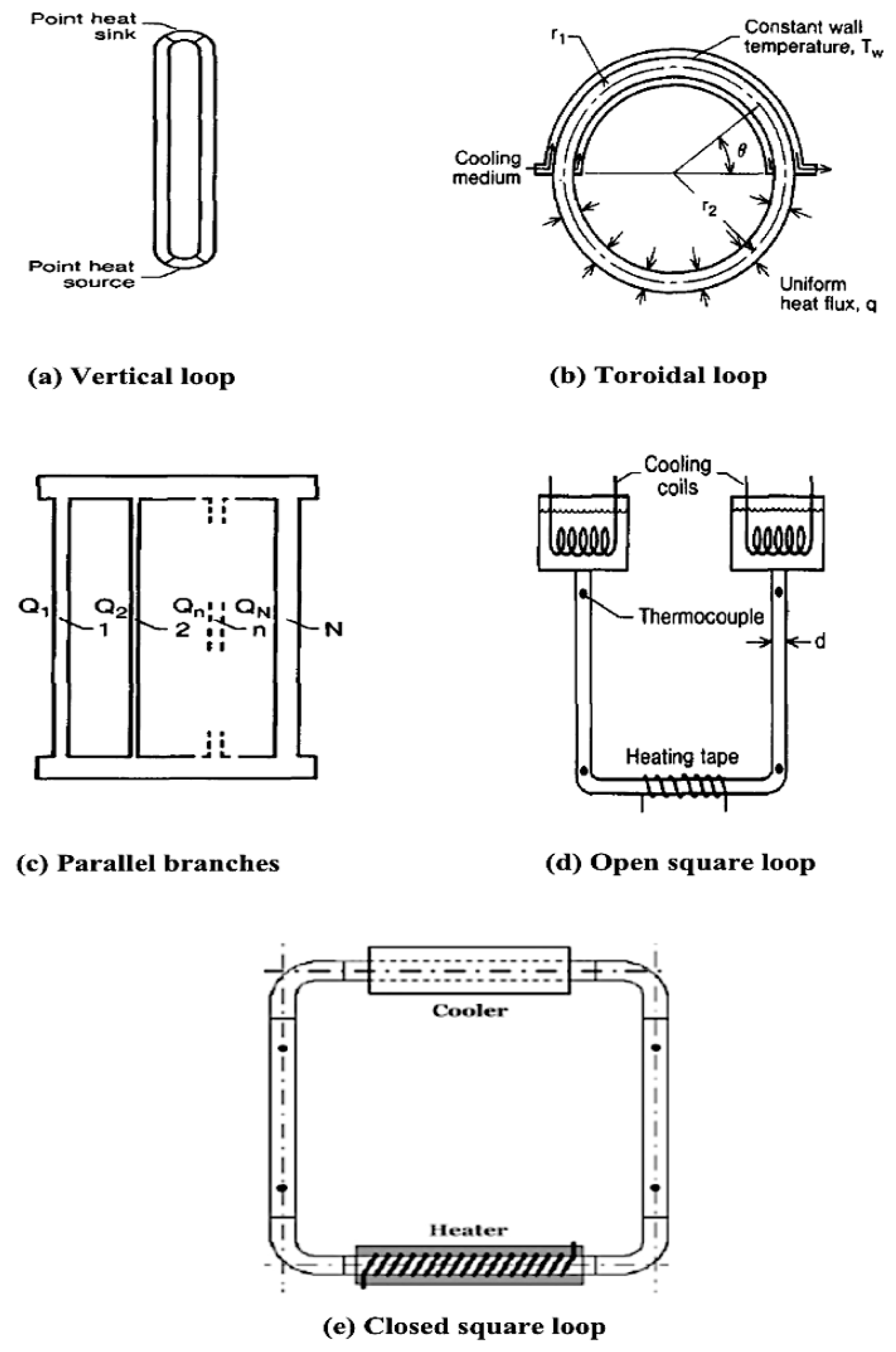
Figure 2.
Experimental Setup for Natural Circulation Loop.
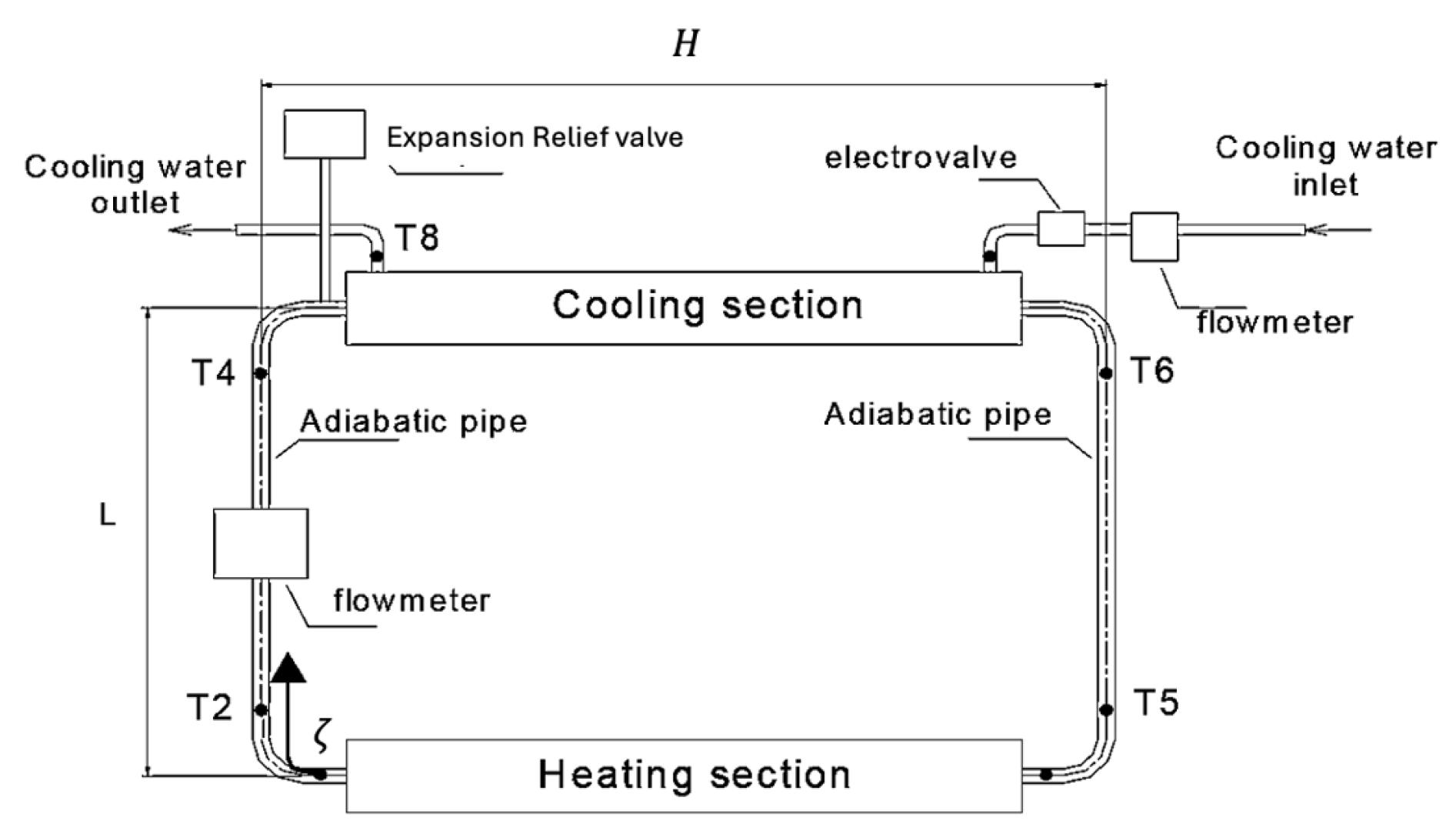
Figure 3.
Eigenmode representation of the system: Stability and Controllability (PBH Test).
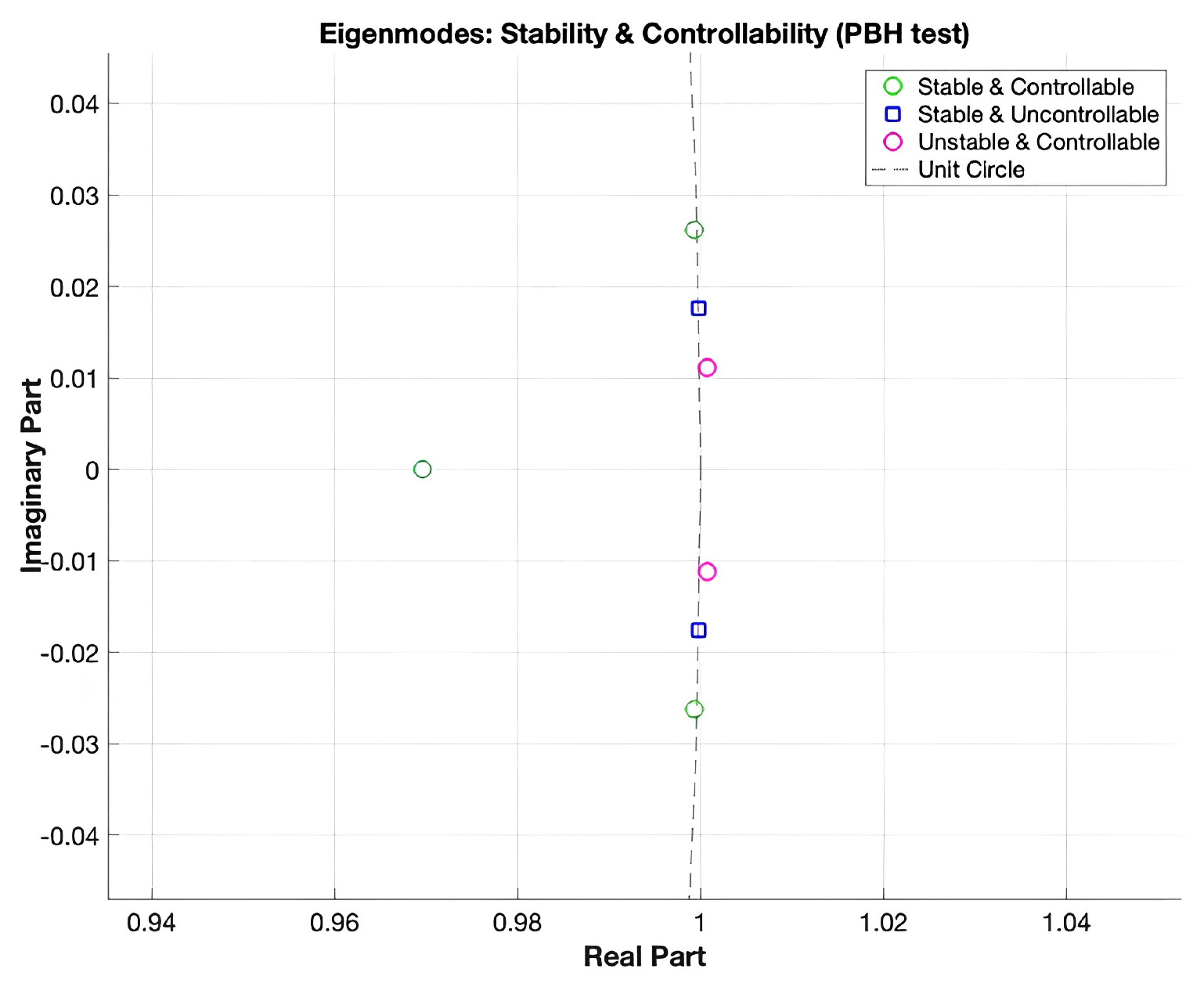
Figure 4.
Estimated states and control input variables for optimal controllers.
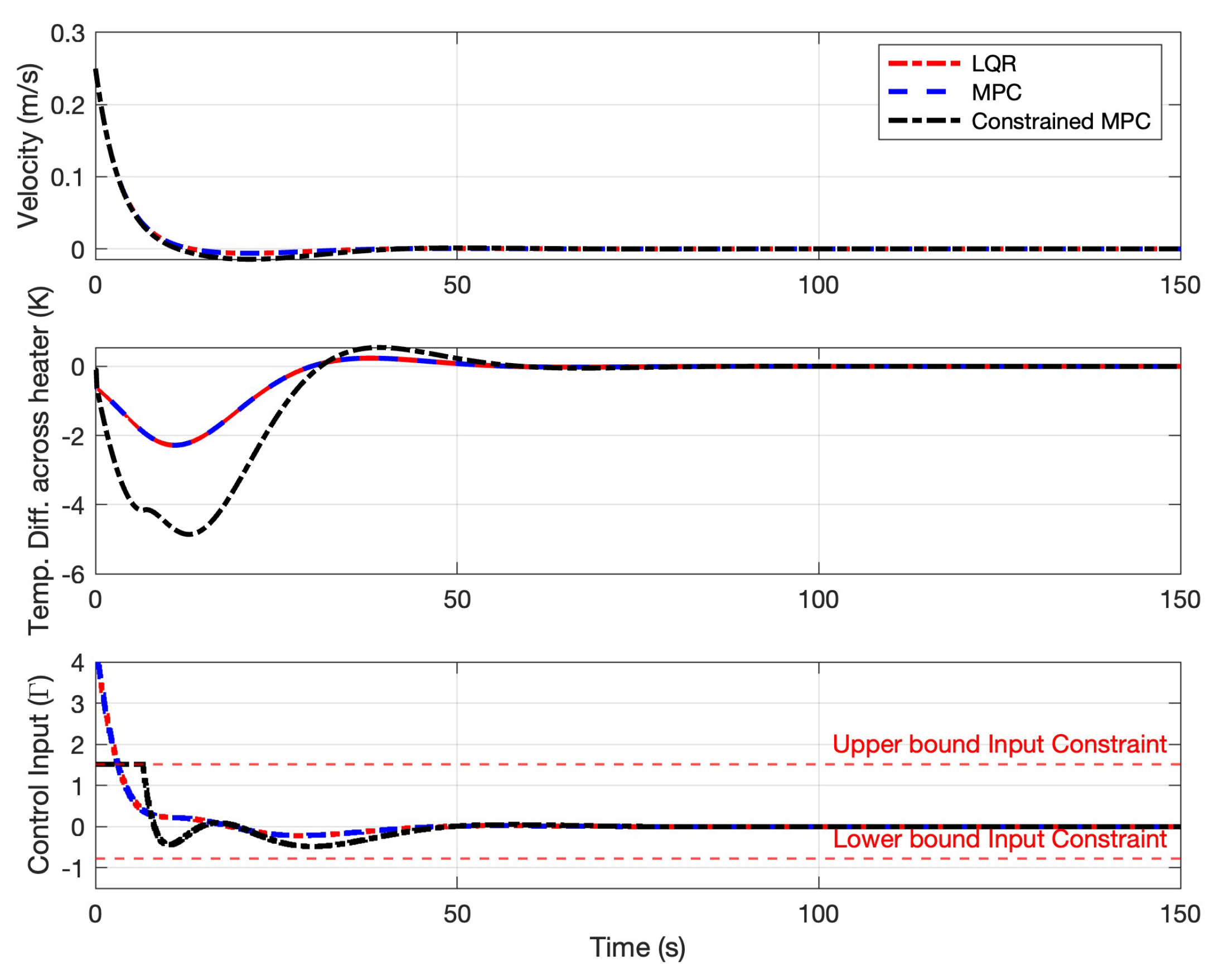
Figure 5.
States and input profiles applying control actions after: (a) 100 seconds (b) 150 sec (c) 200 sec(d) 250 sec.
Figure 5.
States and input profiles applying control actions after: (a) 100 seconds (b) 150 sec (c) 200 sec(d) 250 sec.
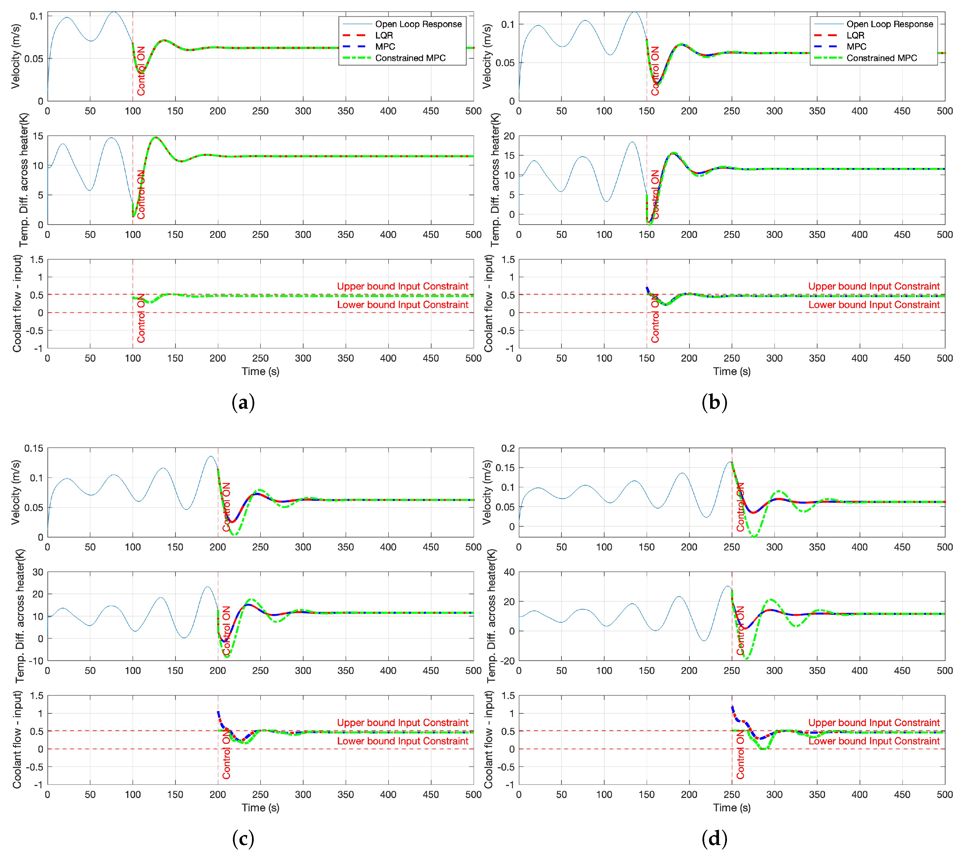

Table 1.
Dimensions of the Experimental Setup.
| Section Name | Dimensions (mm) | Material |
|---|---|---|
| Vertical Loop Height (L) | 1270 | Glass |
| Horizontal Loop Width (H) | 1780 | Glass |
| Loop | 26 | - |
| Heating Section Length | 800 | Inner Tubes: Copper |
| Cooling Section Length | 1000 | Inner Tubes: Copper |
1 Inner diameter (ID) was assumed constant throughout the loop.
Table 2.
Model Parameters.
| Parameters | Values |
|---|---|
| Volumetric Thermal Expansion | 5.04 x |
| Density | 985 |
| Heat Capacity | 4.183 kJ/kg.K |
| Kinematic Viscosity | 0.5 x |
| Reference Temperature | 55oC |
Disclaimer/Publisher’s Note: The statements, opinions and data contained in all publications are solely those of the individual author(s) and contributor(s) and not of MDPI and/or the editor(s). MDPI and/or the editor(s) disclaim responsibility for any injury to people or property resulting from any ideas, methods, instructions or products referred to in the content. |
© 2025 by the authors. Licensee MDPI, Basel, Switzerland. This article is an open access article distributed under the terms and conditions of the Creative Commons Attribution (CC BY) license (http://creativecommons.org/licenses/by/4.0/).
Copyright: This open access article is published under a Creative Commons CC BY 4.0 license, which permit the free download, distribution, and reuse, provided that the author and preprint are cited in any reuse.


