
Submitted:
18 August 2025
Posted:
18 August 2025
You are already at the latest version
Abstract
This paper deals with a class of interval-valued multiobjective optimization problems (IVMOPs). The conjugate-descent (CD) direction is defined to introduce the CD-type conjugate direction algorithm for IVMOPs. We perform the convergence analysis
and establish that the algorithm exhibits a linear rate of convergence under certain suitable assumptions. We further investigate its worst-case complexity. Several numerical examples, including a large-scale problem, are provided to demonstrate the efficacy of the proposed algorithm. To the best of our knowledge, the CD-type conjugate direction algorithm is introduced for the first time to solve a class of IVMOPs.
Keywords:
Interval-valued optimization
; Conjugate Descent method
; Multiobjective optimization
; Conjugate direction algorithm
MSC: 65G40; 26E35; 65K05; 90B50; 90C25; 90C30
1. Introduction
Multiobjective optimization problems (MOPs) are concerned with the simultaneous optimization of two or more mutually conflicting objective functions. Several authors have explored the MOPs in different frameworks (see [1,2,3,4,5,6,7]). In fields like engineering and management sciences (see [8,9]), problems frequently involve imprecise or uncertain data. Such uncertainty may arise from factors including unknown future events, measurement or manufacturing errors, or incomplete information during model formulation [10,11]. In these situations, uncertain parameters or objective functions are often modeled using intervals. When the uncertainties in the objective functions of MOPs are expressed as intervals, the resulting formulations are known as interval-valued multiobjective optimization problems (IVMOPs). Various methods have been developed to handle IVMOPs. For instance, a class of IVMOPs have been studied in [13] by transforming them into their corresponding deterministic MOPs and establishing the relationships between the solutions of IVMOPs and MOPs. In [14], Newton’s method has been proposed to solve IVMOPs, assuming the objective functions possess twice continuous generalized Hukuhara (gH)-differentiability with a positive definite gH-Hessian. Subsequently, the quasi-Newton method for IVMOPs has been introduced in [15]. For recent developments and an updated survey of IVMOPs, we refer to (see [16,17,18]).
The conjugate direction method serves as a powerful tool in optimization, extensively applied to systems of linear equations and diverse optimization problems. Numerous real-world challenges across different fields of modern research, including inverse engineering problems [19], electromagnetic scattering problems [20], and geophysical inversion problems [21], have been successfully addressed employing this method. Hestenes and Stiefel [22] first introduced the conjugate direction method to solve linear systems. Subsequently, several researchers have introduced various versions of conjugate direction methods to solve single-objective as well as multiobjective optimization problems (see [23,24,25,26]). For instance, Fletcher [27] developed the conjugate-descent (CD) method to solve scalar-objective optimization problems. Later, Pérez and Prudente [28] introduced the CD conjugate direction algorithm to solve a class of MOPs. From the above discussions, it is evident that the CD-type conjugate direction method has not yet been introduced to solve IVMOPs. The main aim of this article is to bridge the aforementioned research gap.
Motivated by the works of [27,28], in this article, we investigate a class of IVMOPs and introduce a CD-type conjugate direction algorithm for solving them. We perform the convergence analysis and establish the linear order of convergence of the sequence obtained from the algorithm. Moreover, we investigate the worst-case complexity of the proposed algorithm. Finally, we furnish several numerical examples, including a large scale problem, to illustrate the efficacy of our proposed algorithm.
The key contributions and unique aspects of this article are threefold. Firstly, the results established in this paper generalize several well-known algorithms from the literature. In particular, we generalize the work of Pérez and Prudente [28] on the CD method from MOPs to IVMOPs. Furthermore, we generalize the results of Fletcher [27] for real-valued optimization problems to IVMOP. Secondly, if the conjugate parameter in the proposed algorithm is set to zero and if every component of the objective function of the IVMOP is a real-valued function rather than an interval-valued function, the proposed algorithm coincides with the steepest descent-type algorithm for MOPs introduced by Fliege and Svaiter [29]. Thirdly, it is imperative to note that the proposed CD algorithm is applicable to any IVMOPs where the objective function possesses continuous gH-differentiability. However, Newton’s and quasi-Newton methods proposed in [14,15] require the objective function of the IVMOPs to satisfy twice continuously gH-differentiability. In view of the above fact, our proposed algorithm could be applied to solve a wider class of optimization problems as compared to the algorithms introduced in [14,15].
We design the remainder of this article as follows: Section 2 presents some fundamental definitions and key results. In Section 3, we consider an IVMOP and introduce a CD-type conjugate direction algorithm for solving it. We perform the convergence analysis and establish the linear order of convergence of the sequence obtained from the proposed algorithm. We further investigate the worst-case complexity of the algorithm. To demonstrate the efficacy of the proposed algorithm, we present several numerical examples in Section 4. Finally, Section 5 presents our conclusions and outlines future research directions.
2. Preliminaries
The notations are employed to represent the set of natural numbers and Euclidean space of dimension m, respectively, throughout this article. Let and . Then, and represent the open and closed balls of radius r having center at , respectively. Let , and let denote the identity matrix. For , represents the positive semidefiniteness of .
Let , . Then, the notations mentioned below will be employed:
Let . For any , the symbols and are defined as follows:
provided that the above limits exist.
Assume that for each and , and exist. Then, we define:
Let and denote the sets
respectively.
Let . Then, represents the following interval:
If then is called degenerate interval.
Let , and . We define the subsequent algebraic operations (see [14]):
The following definition of interval norm is from [14].
Definition 1.
Let . The interval norm is defined below:
For , , the following inequalities will be employed:
Let , . The order relations and on and are defined below:
The following definitions are from [15].
Definition 2.
Let , and be arbitrary intervals in . The generalized Hukuhara difference of and is given by:
The interval-valued function is defined below:
Definition 3.
The function χ is called continuous at provided for any , some exists satisfying:
The following definition of gH-Lipschitz continuity is from [32].
Definition 4.
The function χ is called gH-Lipschitz continuous on with Lipschitz constant , provided some constant exists, satisfying:
Remark 1.
Let defined below:
In view of Definition 4, we yield that if χ is gH-Lipschitz continuous on with Lipschitz constant , then is also possess Lipschitz continuity on with Lipschitz constant .
The following definitions and theorem are from [31].
Definition 5.
Let . If the limit
exists, then we say that χ possesses gH-directional derivative at along the direction , denoted by .
Definition 6.
Let the functions and be given by:
The function χ is said to be gH-differentiable at if, there exist , and error functions such that , and for all the following hold:
and
χ is said possess the gH-differentiable on provided it is gH-differentiable at every .
Theorem 1.
If χ possesses gH-differentiability at , then for all , one of the following statements holds:
- (i)
- and both exist and
- (ii)
-
and exist and satisfy:Moreover,
The following definition is from [32].
Definition 7.
Let χ be gH-differentiable on . The gH-gradient of χ on at is given below:
where is the j-th canonical direction in .
The subsequent proposition is from [14].
Proposition 1.
If χ possesses k-times gH-differentiability at , then , defined in (1), also possesses k-times differentiablility at .
Now, we define the interval-valued vector function as follows:
where each are given below:
The definitions from [16] play a significant role in our forthcoming discussions.
Definition 8.
Let and . Suppose each component possesses gH-directional derivatibility at . Then, is a critical point of Γ provided no exists, satisfying:
where .
Definition 9.
A vector is called descent direction of Γ at a point provided some exists, satisfying:
3. CD-Type Conjugate Direction Method for IVMOP
This section is devoted to introduce the CD-type conjugate direction algorithm to solve an IVMOP. We perform the convergence analysis and establish the linear rate of convergence of the sequence obtained from the proposed algorithm. We investigate further the worst-case complexity of the proposed algorithm, under certain mild assumptions.
Consider the IVMOP, given below:
where the functions . Unless specified otherwise, we assume that are continuously gH-differentiable functions.
The following definitions are from [14].
Definition 10.
An element is called effective (respectively, weak effective) solution of IVMOP provided no exists, satisfying:
Throughout the remainder of this article, denotes the set of all critical points of .
In light of Definition 8, it follows that if , then there exists , satisfying:
To determine the descent direction at , we consider following problem from [16]:
where , and the uniqueness of the solution of is straightforward.
For each , let denote the feasible set of problem , and let denote an arbitrary feasible point. We then define the functions and as follows:
Henceforth, for any , the optimal solution of will be signified by .
The lemmas provided below are from Upadhyay et al. [16].
Lemma 1.
Let . Then the following properties hold:
- (i)
- , provided .
- (ii)
- , provided .
Lemma 2.
If () are locally strongly convex (locally convex, respectively) at , then is a locally effective (locally weak effective, respectively) solution of IVMOP.
Lemma 3.
If , then is a descent direction of Γ at .
We define as follows:
where for each , denotes the upper bound of the interval
The lemma provided below relates to .
Lemma 4.
For every , the following relation holds:
Proof.
Since , the following holds:
This implies that:
If , then some exists, satisfying:
Define
This implies
contradicting the assumption that is a solution to . Therefore
This completes the proof. □
Let and . If , then the conjugate-descent (CD) direction at is defined as follows:
where for , is given by
Remark 2.
The next theorem demonstrates that, under suitable hypotheses, the direction defined in (9) at any is a descent direction.
Theorem 2.
Let and suppose that . If the parameter satisfies the following conditions:
where, the function Λ is defined in (3) and , then is a descent direction of Γ at .
Proof.
Given that each function () is continuously gH-differentiable, to show is a descent direction it suffices to show that
Let be fixed. Consider the expression:
Expanding the first term we get:
Now, we consider the two possible cases:
Case 1: Using Equation (14), it follows that
Since , therefore from Lemma 1 we have
Also, from Lemma 4 we get:
Case 2: Using Equation (14), it follows that
Similarly it can be shown that
This completes the proof. □
We define the functions as follows:
The functions , as defined in (23), are employed in the subsequent analysis.
Remark 3.
In light of Theorem 2, if and satisfies (11), then the direction , as defined by (9), serves as a descent direction at . Therefore,
It follows that
The following Armijo-like line search for is from [32].
Let be such that defines a descent direction of at . For a given , a step length is called admissible provided it satisfies the subsequent condition:
Remark 4.
Let satisfy the Armijo condition (25) for Γ at along direction with parameter θ. Then, the functions satisfies:
For the numerical implementation of the Armijo-like search method, we incorporate it with a backtracking strategy. The line search is initialized with and proceeds as follows:
- (a)
- (b)
- Else, set and return to Step (a).
We now present a CD-type conjugate direction algorithm for IVMOPs.
| Algorithm 1 CD-type conjugate direction algorithm for solving IVMOP |
|
Remark 5.
Observe that if Algorithm 1 terminates after a finite number of iterations, its final iterate is an approximate critical point. Consequently, it is relevant to perform the convergence analysis of Algorithm 1 for the case of infinite sequence, that is, for all .
The theorem, provided below, establishes the convergence analysis of the sequence obtained from Algorithm 1.
Theorem 3.
Suppose the set
is bounded. Then, every accumulation point of belongs to the set .
Proof.
In view of (25), the following inequality is satisfied for all :
Therefore, from Remark 3 we obtain
This implies
Hence, . From the given hypotheses, we have the boundedness of , which gives the boundedness of the sequence . This ensures that it has at least one accumulation point, , say. We prove that .
Now, using (25) we have
Since therefore, exists. Here two cases may arise:
Case 1:. Since be an accumulation point of and , therefore, a subsequence of exists, satisfying:
We want to prove . On the contrary, assume that . Therefore, there are and such that
Because is continuous for all , and converges to , therfore from (32) there exists such that for all we have
Taking and using (33) we obtain
From (34), some exists such that
From (35) we obtain . Therefore, due to the fact that is a solution of we obtain
Since is a solution of , from (36) we obtain
For all we have
Now consider . If , then we have
If , then using (3) we have
Therefore, using (36) we obtain:
From (34) we have and since , therefore , hence from (47) we obtain:
which contradicts Equation (31).
Case 2:.
This implies . Let be fixed. Then, some exists, satisfying:
Therefore, for the Equation (25) does not hold. That is, the following does not hold for all
Hence, passing limit along suitable subsequence there exists such that for sufficiently large enough s we have
yields a contradiction. □
The subsequent lemma is from [32].
Lemma 5.
Assume that each function possesses twice continuous gH-differentiability and satisfies gH-Lipschitz continuity with a Lipschitz constant on . Then, the functions are also twice continuously differentiable and Lipschitz continuous on , with a Lipschitz constant .
The next theorem establishes that the sequence obtained from Algorithm 1 exhibits linear order convergence.
Theorem 4.
Let be the sequence obtained from Algorithm 1, and assume the set
is bounded. Assume that possesses twice continuous gH-differentiability on , and its gH-gradient possesses gH-Lipschitz continuity on with Lipschitz constant . Further, let for some , and define . Then the sequence converges linearly.
Proof.
In view of the boundedness of and Theorem 3, the sequence obtained from Algorithm 1 converges to a critical point of , say . Since the functions possess twice continuous gH-differentiability, Lemma 5 implies that the functions are twice continuously differentiable. Therefore, by employing the second-order Taylor expansion for each with (see [30]) we obtain:
for some . Since , it follows from (49) that:
Using (28) we have
Utilizing the mean value theorem (see [30]) on the right-hand side of (52), leads to the following:
for some . Given that are gH-Lipschitz continuous with Lipschitz constant , Lemma 5 implies that the are Lipschitz continuous with constant . Hence, from (53) we obtain
As is a critical point, there exists such that the following inequality holds:
The following lemma plays a pivotal role in our subsequent discussions.
Lemma 6.
Suppose that possess gH-Lipschitz continuity with Lipschitz constant and assume some exists, satisfying:
Then every step length computed in Algorithm 1 satisfies
Proof.
In view of Remark 4 and the fact that is the step length, there exists such that:
By Lemma 5 and the gH-Lipschitz continuity of with Lipschitz constant we obtain is Lipschitz continuous with Lipschitz constant . Consequently, the following inequality holds:
Substituting into (59) yields:
Equivalently,
Since and it follows that
Furthermore, by Remark 3, the following inequality holds:
Since for every , therefore (63) implies:
This completes the proof. □
In the forthcoming theorem, the worst-case complexity of the sequence obtained from Algorithm 1 is investigated.
Theorem 5.
Let every assumption of Theorem 4, along with the assumptions of Lemma 6, be satisfied. Let be the sequence obtained from Algorithm 1. If, for any , the algorithm requires at most iterations to obtain an iterate such that , then
Proof.
Given that the sequence is obtained from Algorithm 1 and the set is bounded, Theorem 3 implies that the sequence converges to . Further, since the functions possess twice continuous gH-differentiability, Lemma 5 implies that also possess twice continuous differentiability. Given the boundedness of , some exists, satisfying:
Furthermore, since () are continuous on the compact set , some exists satisfying:
As represents the step size in Algorithm 1, Remark 4 implies that, for each the following inequality holds
Since , therefore using Remark 3 we obtain:
where . Equivalently,
Since for all , it follows from (67) that:
By applying the mean value theorem (see [30]) on the left-hand side of (68) we obtain
for some . Since , it follows that
Moreover, by invoking Theorem 4 and (71) we arrive at the following inequality:
Now, applying Lemma 6 to (72) it follows that:
Assume now that for the first iterations the condition holds. Then, using (73) we obtain:
By taking the logarithm of both sides of the above inequality we obtain:
This implies
This completes the proof. □
4. Numerical Experiments
An example involving a locally convex IVMOP is presented below to illustrate the significance of Algorithm 1.
Example 1.
Examine the following IVMOP:
where are defined as follows:
It can be verified that is a critical point of Γ in (Q1). Moreover, since and are locally convex at , Lemma 2 implies that is a locally weak effective solution of (Q1). We solve (Q1) using Algorithm 1, starting from the initial point and termination condition . The computational results of Algorithm 1 are presented in Table 1.
The result shown in Step 16 of Table 1 ensures that the sequence converges to , which is a locally weak effective solution of (Q1).
It is important to highlight that a locally weak efficient solution of an IVMOP is not necessarily an isolated point. Nevertheless, when Algorithm 1 is executed from a specific starting point, it may converge to one such solution. To generate a set of approximate locally weak efficient solutions in Example 1, a multi-start strategy is adopted. Specifically, 50 uniformly distributed random initial points are generated using MATLAB’srandfunction. Algorithm 1 is then independently executed from each of these initial points, with the termination condition defined as . The iterative sequences generated from these initializations are visualized in Figure 1.
Remark 6.
It is important to note that, in (Q1), is non-convex and possesses twice continuous gH-differentiability. As a result, the Newton’s method for IVMOPs proposed in [14] is not applicable to solve (Q1). Nevertheless, Example 1 illustrates that Algorithm 1 solves (Q1) effectively.
It is significant to note that the Newton’s and quasi-Newton methods proposed in [14,15] are applicable to solve a specific class of IVMOPs, where the objective functions possess twice continuous gH-differentiability. In contrast, Algorithm 1 needs to be continuously gH-differentiable. Consequently, Algorithm 1 can be applied to a broader class of IVMOPs than the methods proposed in [14,15]. This is demonstrated in the following example.
Example 2.
Examine the following IVMOP:
where and are defined as follows:
and
Evidently, is continuously gH-differentiable; however, it does not possess twice continuous gH-differentiability. As a matter of the fact that, Newton’s method introduced in [14] are not applicable for solving (Q2). Nevertheless, (Q2) is solved employing Algorithm 1, implemented in the MATLAB. We now apply Algorithm 1 to solve (Q2). The initial point and the stopping condition criteria are set to be and , respectively. The computational results obtained using Algorithm 1 are presented in Table 2.
As indicated in Step 36 of Table 2, Algorithm 1 generates a sequence that converges to the approximate critical point for the objective function in (Q2).
In the next example we investigate a large-scale IVMOP.
Example 3.
Examine the following IVMOP:
where is defined as follows:
A random initial point, generated using MATLAB’srand(n,1)function, is used to initialize Algorithm 1. The termination criterion is defined as . From Table 3 we find the iteration counts and the associated computational times required by Algorithm 1 to solve (Q3) for different values of n.
5. Conclusions and Future Research Directions
In this article, we investigated a class of IVMOPs. We defined the conjugate-descent (CD) direction to introduce CD-type conjugate direction algorithm for IVMOPs. We performed the convergence analysis and established the linear rate of convergence of the sequence obtained from the algorithm, under appropriate assumptions. Moreover, the worst-case complexity of the proposed algorithm has been investigated.
The results established in this paper generalize several significant results existing in the literature. In particular, the results derived in this paper generalize the corresponding results of Pérez and Prudente [28] on CD conjugate direction algorithm from MOPs to a more general class of optimization problems, namely, IVMOPs. Moreover, if the conjugate parameter in the proposed algorithm is set to be zero, and if every component of the objective function of the IVMOP is a real-valued function rather than an interval-valued function, then the proposed algorithm coincides with the steepest descent-type method for MOPs introduced by Fliege and Svaiter [29]. We have conducted numerical experiments to illustrate the fact that the proposed algorithm is applicable to solve a broader class of optimization problems as compared to the methods existing in the literature (see Upadhyay et al. [14,15]).
The findings of this research open several avenues for future exploration. On one hand, the results of this paper could be further generalized to the class of nonsmooth IVMOPs. On the other hand, given the advantages of developing optimization algorithms in the framework of Riemannian manifolds (see [33]), the results of this paper could be generalized to the Riemannian manifold setting.
Author Contributions
Conceptualization, B.B.U. and R.K.P.; methodology, B.B.U., R.K.P.; validation, B.B.U., R.K.P., S.P., and I.M.S.-M.; formal analysis, B.B.U., R.K.P., and S.P.; writing-review and editing, B.B.U., R.K.P., and S.P.; supervision, B.B.U.
Funding
The first author would like to thank receives financial support from the University Grants Commission, New Delhi, India (UGC-Ref. No.: 1213/(CSIR-UGC NET DEC 2017)). The third author extends gratitude to the Ministry of Education, Government of India, for their financial support through the Prime Minister Research Fellowship (PMRF), granted under PMRF ID-2703573.
Data Availability Statement
The authors confirm that no data, text, or theories from others are used in this paper without proper acknowledgement.
Acknowledgments
The authors would like to thank the anonymous reviewers for their constructive suggestions, which have substantially improved the paper in its present form.
Conflicts of Interest
The authors confirm that there are no actual or potential conflicts of interest related to this article.
References
- Miettinen, K. Nonlinear Multiobjective Optimization; Springer Science & Business Media: Berlin/Heidelberg, Germany, xvii, 298 p. 1999.
- Diao, X.; Li, H.; Zeng, S.; Tam, V.W.; Guo, H. A Pareto multi-objective optimization approach for solving time-cost-quality tradeoff problems. Technol. Econ. Dev. Econ. 2011, 17, 22–41. [Google Scholar] [CrossRef]
- Guillén-Gosálbez, G. A novel MILP-based objective reduction method for multi-objective optimization: Application to environmental problems. Comput. Chem. Eng. 2011, 35, 1469–1477. [Google Scholar] [CrossRef]
- Bento, G.C.; Melo, J.G. Subgradient method for convex feasibility on Riemannian manifolds. J. Optim. Theory Appl. 2012, 152, 773–785. [Google Scholar] [CrossRef]
- Upadhyay, B.B.; Stancu-Minasian, I.M.; Mishra, P.; Mohapatra, R.N. On generalized vector variational inequalities and nonsmooth vector optimization problems on Hadamard manifolds involving geodesic approximate convexity. Adv. Nonlinear Var. Inequal. 2022, 25, 1–25. [Google Scholar]
- Upadhyay, B.B.; Singh, S.K.; Stancu-Minasian, I.M.; Rusu-Stancu, A.M. Robust optimality and duality for nonsmooth multiobjective programming problems with vanishing constraints under data uncertainty. Algorithms 2024, 17(11), 482. [Google Scholar] [CrossRef]
- Upadhyay, B.B.; Poddar, S.; Yao, J. C.; Zhao, X. Inexact proximal point method with a Bregman regularization for quasiconvex multiobjective optimization problems via limiting subdifferentials. Ann. Oper. Res. 2025, 345, 417–466. [Google Scholar] [CrossRef]
- Qiu, D.; Jin, X.; Xiang, L. On solving interval-valued optimization problems with TOPSIS decision model. Eng. Lett. 2022, 30, 1101–1106. [Google Scholar]
- Lanbaran, N.M.; Celik, E.; Yiğider, M. Evaluation of investment opportunities with interval-valued fuzzy TOPSIS method. Appl. Math. Nonlinear Sci. 2020, 5, 461–474. [Google Scholar] [CrossRef]
- Beer, M.; Ferson, S.; Kreinovich, V. Imprecise probabilities in engineering analyses. Mech. Syst. Signal Process, 2013, 37, 4–29. [Google Scholar] [CrossRef]
- Chaudhuri, A.; Lam, R.; Willcox, K. Multifidelity uncertainty propagation via adaptive surrogates in coupled multidisciplinary systems. AIAA J. 56, 235–249. [CrossRef]
- Zhang, J.; Li, S. The portfolio selection problem with random interval-valued return rates. Int. J. Innov. Comput. Inf. Control 2009, 5, 2847–2856. [Google Scholar]
- Kumar, P.; Bhurjee, A.K. Multi-objective enhanced interval optimization problem. Ann. Oper. Res. 2022, 311, 1035–1050. [Google Scholar] [CrossRef]
- Upadhyay, B.B.; Pandey, R.K.; Liao, S. Newton’s method for interval-valued multiobjective optimization problem. J. Ind. Manag. Optim. 2024, 20, 1633–1661. [Google Scholar] [CrossRef]
- Upadhyay, B.B.; Pandey, R.K.; Pan, J.; Zeng, S. Quasi-Newton algorithms for solving interval-valued multiobjective optimization problems by using their certain equivalence. J. Comput. Appl. Math. 2024, 438, 115550. [Google Scholar] [CrossRef]
- Upadhyay, B.B.; Pandey, R.K.; Zeng, S. A generalization of generalized Hukuhara Newton’s method for interval-valued multiobjective optimization problems. Fuzzy Sets Syst. 2024, 492, 109066. [Google Scholar] [CrossRef]
- Zhang, Z.; Wang, X.; Lu, J. Multi-objective immune genetic algorithm solving nonlinear interval-valued programming. Eng. Appl. Artif. Intell. 2018, 67, 235–245. [Google Scholar] [CrossRef]
- Upadhyay, B.B.; Pandey, R.K.; Zeng, S.; Singh, S.K. On conjugate direction-type method for interval-valued multiobjective quadratic optimization problems. Numer. Algorithms 2024. [Google Scholar] [CrossRef]
- Pandey, V.; Bekele, A.; Ahmed, G.M.S.; Kanu, N.J. An application of conjugate gradient technique for determination of thermal conductivity as an inverse engineering problem. Mater. Today Proc. 2021, 47, 3082–3087. [Google Scholar] [CrossRef]
- Sarkar, T.; Rao, S. : The application of the conjugate gradient method for the solution of electromagnetic scattering from arbitrarily oriented wire antennas. IEEE Trans. Antennas Propag. 1984, 32, 398–403. [Google Scholar] [CrossRef]
- Frank, M.S.; Balanis, C.A. A conjugate direction method for geophysical inversion problems. IEEE Trans. Geosci. Remote Sens. 2007, 25, 691–701. [Google Scholar] [CrossRef]
- Hestenes, M.R.; Stiefel, E. Methods of conjugate gradients for solving linear systems. J. Res. Natl. Bur. Stand. 1952, 49, 409–436. [Google Scholar] [CrossRef]
- Fletcher, R.; Reeves, C.M. Function minimization by conjugate gradients. Comput. J. 1964, 7, 149–154. [Google Scholar] [CrossRef]
- Polak, E. , Ribieŕe, G.: Note sur la convergence de méthodes de directions conjuguées. Rev. Fr. Inform. Recherche Opér. 1969, 3, 35–43. [Google Scholar]
- Khoda, K.M.; Liu, Y.; Storey, C. Generalized Polak-Ribieŕe algorithm. J. Optim. Theory Appl. 1992, 75, 345–354. [Google Scholar] [CrossRef]
- Zhang, L.; Zhou, W.J.; Li, D.H. A descent modified Polak-Ribieŕe-Polyak conjugate gradient method and its global convergence. IMA J. Numer. Anal. 2006, 26, 629–640. [Google Scholar] [CrossRef]
- Fletcher, R. Unconstrained Optimization; Pract. Methods Optim., Vol. 1; John Wiley: New York, 1980. [Google Scholar]
- Pérez, L.R.; Prudente, L.F. Nonlinear conjugate gradient methods for vector optimization. SIAM J. Optim. 2018, 28, 2690–2720. [Google Scholar] [CrossRef]
- Fliege, J.; Svaiter, B.F. Steepest descent methods for multicriteria optimization. Math. Methods Oper. Res. 2000, 51, 479–494. [Google Scholar] [CrossRef]
- Apostol, T.M. Multi-Variable Calculus and Linear Algebra with Applications to Differential Equations and Probability; Wiley: New York, NY, USA, 1969. [Google Scholar]
- Stefanini, L.; Bede, B. Generalized Hukuhara differentiability of interval-valued functions and interval differential equations. Nonlinear Anal. 2009, 71, 1311–1328. [Google Scholar] [CrossRef]
- Pandey, R.K.; Upadhyay, B.B.; Poddar, S.; Stancu-Minasian, I.M. Hestenes-Stiefel-type conjugate direction algorithm for interval-valued multiobjective optimization problems. Algorithms 2025, 18, 381. [Google Scholar] [CrossRef]
- Upadhyay, B.B.; Poddar, S.; Ferreira, O. P.; Zhao, X.; Yao, J.C. An inexact proximal point method with quasi-distance for quasiconvex multiobjective optimization problems on Riemannian manifolds. Numer. Algorithms 2025, 1–51. [Google Scholar] [CrossRef]
Figure 1.
Approximate locally weak effective solutions obtained from 50 uniformly random initial points.
Figure 1.
Approximate locally weak effective solutions obtained from 50 uniformly random initial points.
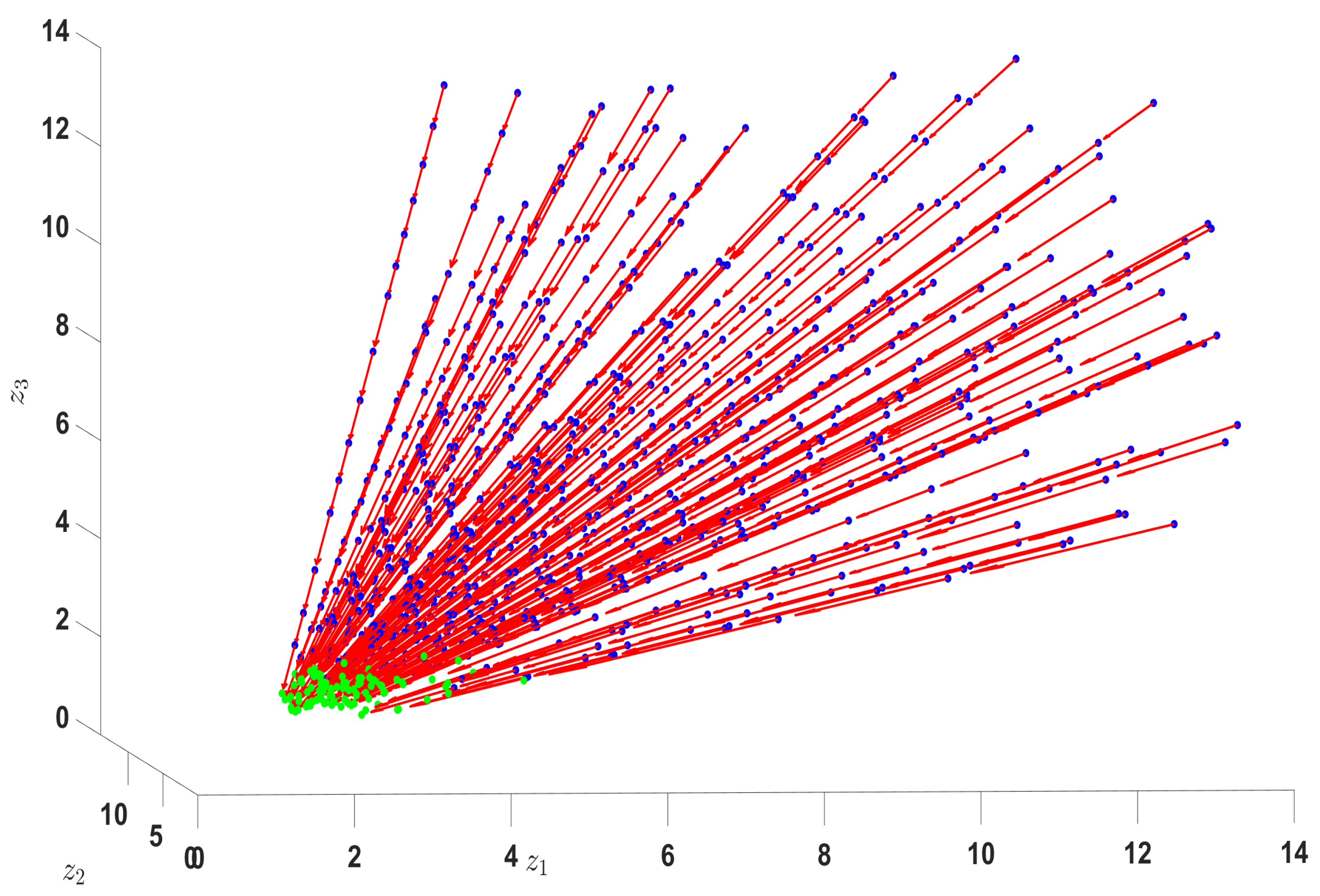

Table 1.
Computational results obtained from Algorithm 1 for solving (Q1).
| s | ||||
| 0 | 1050 | |||
| 1 | ||||
| 2 | ||||
| 3 | ||||
| 4 | ||||
| 5 | ||||
| 6 | 484 | |||
| 7 | ||||
| 8 | ||||
| 9 | ||||
| 10 | ||||
| 11 | ||||
| 12 | ||||
| 13 | ||||
| 14 | ||||
| 15 | ||||
| 16 |
Table 2.
Computational results obtained from Algorithm 1 for solving (Q2).
| s | ||||
| 0 | ||||
| 1 | ||||
| 2 | ||||
| 3 | ||||
| 4 | ||||
| 5 | ||||
| 6 | ||||
| 7 | ||||
| 8 | ||||
| 9 | ||||
| 10 | ||||
| 11 | ||||
| 12 | ||||
| 13 | ||||
| 14 | ||||
| 15 | ||||
| 16 | ||||
| 17 | ||||
| 18 | ||||
| 19 | ||||
| 20 | ||||
| 21 | ||||
| 22 | ||||
| 23 | ||||
| 24 | ||||
| 25 | ||||
| 26 | ||||
| 27 | ||||
| 28 | ||||
| 29 | ||||
| 30 | ||||
| 31 | ||||
| 32 | ||||
| 33 | ||||
| 34 | ||||
| 35 | ||||
| 36 |
Table 3.
The computational results of Algorithm 1 for the (Q3).
| Number of iterations | Computation times (in seconds) | |
| 100 | 2183 | |
| 130 | 2611 | 3225 |
| 160 | 4518 | 6337 |
| 190 | 3422 | 5442 |
| 220 | 3667 | 6750 |
| 250 | 3896 | 7889 |
| 280 | 2363 | 5705 |
| 310 | 2460 | 7059 |
| 340 | 3549 | 1062 |
| 370 | 4325 | |
| 400 | 3004 |
Disclaimer/Publisher’s Note: The statements, opinions and data contained in all publications are solely those of the individual author(s) and contributor(s) and not of MDPI and/or the editor(s). MDPI and/or the editor(s) disclaim responsibility for any injury to people or property resulting from any ideas, methods, instructions or products referred to in the content. |
© 2025 by the authors. Licensee MDPI, Basel, Switzerland. This article is an open access article distributed under the terms and conditions of the Creative Commons Attribution (CC BY) license (http://creativecommons.org/licenses/by/4.0/).
Copyright: This open access article is published under a Creative Commons CC BY 4.0 license, which permit the free download, distribution, and reuse, provided that the author and preprint are cited in any reuse.


