
Submitted:
17 May 2025
Posted:
20 May 2025
You are already at the latest version
Abstract
This article investigates a class of interval-valued multiobjective optimization problems (IVMOPs, in short). We define the Hestenes-Stiefel (HS, in short) direction for the objective function of IVMOPs and establish that it has a descent property at noncritical points. An Armijo-like line search is employed to determine an appropriate step size. We present an HS-type conjugate direction algorithm for IVMOPs and establish the convergence of the sequence generated by the algorithm. Moreover, we furnish several numerical examples, including convex, locally convex, and large-scale IVMOPs, to demonstrate the effectiveness of our proposed algorithm and solve them by employing MATLAB R2024a. To the best of our knowledge, the HS-type conjugate direction method has not yet been explored for the class of IVMOPs.
Keywords:
Hestenes-Stiefel method
; interval-valued optimization
; Generalized Hukuhara derivative
; conjugate direction method
; multiobjective optimization
MSC: 90B50; 65G40; 90C30; 90C25; 26E35; 65K05
1. Introduction
Multiobjective optimization problems (MOPs, in short) involve the simultaneous optimization of two or more conflicting objective functions. Vilfredo Pareto [1] introduced the concept of Pareto optimality in the context of economic systems. A solution is called Pareto optimal or efficient, if none of the objective functions can be improved without deteriorating some of the other objective values (see, [2]). MOPs arise in scenarios where trade-offs are required, such as balancing cost and quality in business operations or improving efficiency while reducing environmental impact in engineering (see, [3,4]). As a consequence, various techniques and algorithms have been proposed to solve MOPs in different frameworks (see, [5,6,7]). For a more detailed discussion on MOPs, we refer to [2,8] and the references cited therein.
In many real world problems arising in engineering, science and related fields, we often encounter data that are imprecise or uncertain. This uncertainty can arise from various factors such as unknown future developments, measurement or manufacturing errors, or incomplete information in model development (see, [9,10]). In several optimization problems, the presence of imprecise data or uncertainty in the parameters or the objective functions is modeled as intervals. These optimization problems are termed interval-valued optimization problems (IVOPs, in short). IVOPs have significant applications in various fields, including management, economics and engineering (see, [11,12,13]). The foundational work on IVOPs is attributed to Ishibuchi and Tanaka [14], who investigated IVOPs by transforming them into corresponding deterministic MOPs. Wu [15] derived optimality conditions for a class of constrained IVOPs, employing the notion of Hukuhara differentiability and assuming the convexity hypothesis on the objective and constraint functions. Moreover, Wu [16] developed Karush-Kuhn-Tucker-type optimality conditions for IVOPs and derived strong duality theorems that connect the primal problems with their associated dual problems. Bhurjee and Panda [17] explored IVOPs by defining interval-valued functions in parametric forms. More recently, Roy et al. [18] proposed a gradient based descent line search technique employing the notion of generalized Hukuhara (gH, in short) differentiability to solve IVOPs.
In the theory of mathematical optimization, if the uncertainties involved in the objective functions of MOPs are represented as intervals, the resulting problems are referred to as interval-valued multiobjective optimization problems (IVMOPs, in short). IVMOPs frequently arise in diverse fields such as transportation, economics, and business administration [19,20]. As a result, several researchers have developed various methods to solve IVMOPs. For instance, Kumar and Bhurjee [21] studied IVMOPs by transforming them into their corresponding deterministic MOPs and establishing the relationships between the solutions of IVMOPs and MOPs. Upadhyay et al. [22] introduced Newton’s method for IVMOPs and established the quadratic convergence of the sequence generated by Newton’s method under suitable assumptions. Subsequently, Upadhyay et al. [23] developed quasi-Newton methods for IVMOPs and demonstrated their efficacy in solving both convex and non-convex IVMOPs. For a more comprehensive and updated survey on IVMOPs, see [24,25,26,27] and the references cited therein.
It is well-known that the conjugate direction method is a powerful optimization technique that can be widely employed for solving systems of linear equations and optimization problems (see, [28,29]). It has been observed that several real-life optimization problems emerging in different fields of modern research, such as electromagnetic scattering [30], inverse engineering [31], and geophysical inversion [32]. The conjugate direction method was first introduced by Hestenes and Stiefel [28], who developed the conjugate gradient method to solve a system of linear equations. Subsequently, Pérez and Prudente [29] introduced the HS-type conjugate direction algorithm for MOPs by employing an inexact line search. Wang et al. [33] introduced an HS-type conjugate direction algorithm for MOPs without employing line search techniques, and established the global convergence of the proposed method under suitable conditions. Recently, based on the memoryless Broyden-Fletcher-Goldfarb-Shanno update, Khoshsimaye-Bargard and Ashrafi [34] presented a convex hybridization of the Hestenes-Stiefel and Dai-Yuan conjugate parameters. From the above discussion, it is evident that HS-type conjugate direction methods have been developed to solve single-objective problems as well as MOPs. However, there is no research paper available in the literature that has explored the HS-type conjugate direction method for IVMOPs. The aim of this article is to fill the aforementioned research gaps by developing the HS-type conjugate direction method for a class of IVMOPs.
Motivated by the works of [28,29,33], in this paper, we investigate a class of IVMOPs and define the HS-direction for the objective function of IVMOPs. A descent direction property of the HS-direction is established at noncritical points. To determine an appropriate step size, we employ an Armijo-like line search. Moreover, an HS-type conjugate direction algorithm for IVMOPs is presented, and the convergence of this algorithm is established. Finally, the efficiency of the proposed method is demonstrated by solving various numerical problems employing MATLAB R2024a.
The primary contribution and novel aspect of this article are threefold. Firstly, the results presented in this paper generalize several significant results from existing literature. Specifically, we generalize the results established by Pérez and Prudente [29] on the HS-type method from MOPs to a more general class of optimization problems, namely, IVMOPs. Secondly, if the conjugate parameter is set to zero and if every component of the objective function of the IVMOP is a real-valued function rather than interval-valued function, then the proposed algorithm reduces to the steepest descent algorithm for MOPs, as introduced by Fliege and Svaiter [5]. Thirdly, it is imperative to note that the proposed HS-type algorithm is applicable to any IVMOP, where the objective function is continuously gH-differentiable. However, Newton’s and Quasi-Newton methods proposed by Upadhyay et al. [22,23] require the objective functions of the IVMOPs to be twice continuously gH-differentiable. In view of this fact, our proposed algorithm can be applied to a broader class of optimization problems compared to the algorithms introduced by Upadhyay et al. [22,23].
The rest of the paper is structured as follows. In Section 2, we discuss some mathematical preliminaries that will be employed in the sequel. Section 3 presents an HS-type conjugate direction algorithm for IVMOPs, along with a convergence analysis of the sequence generated by the algorithm. In Section 4, we demonstrate the efficiency of the proposed algorithm by solving several numerical examples via MATLAB R2024a. Finally, in Section 5, we provide our conclusions as well as future research directions.
2. Preliminaries
Throughout this article, the symbol denotes the set of all natural numbers. For , the symbol refers to the -dimensional Euclidean space. The symbol refers to the collection of all negative real numbers. The symbol ∅ is employed to denote an empty set. For any non-empty set and , the notation represents the Cartesian product defined as
Let . Then the symbol is defined as
For , the symbol is defined as
Let . Then, the notations and are used to represent the following sets:
Let . The following notations are employed throughout this article:
For and , we define
and
which denote the one-sided right and left -th partial derivatives of at the point , respectively, assuming the limits defined in (1) and (2) are well-defined.
If for every and , and exist, then we define:
The symbols and are used to denote the following sets:
Let . The symbol represents the following:
The interval is referred to as a degenerate interval if and only if
Let , , and . Corresponding to and , we define the following algebraic operations (see, [22]):
The subsequent definition is from [35].
Definition 1.
Consider an arbitrary set . Then, the symbol represents the norm of and is defined as follows:
For and , we adopt the following notations throughout the article:
Let , . The ordered relations between and are described as follows:
The following definition is from [35].
Definition 2.
For arbitrary intervals and , the symbol represents the gH-difference between and and is defined as
The notion of continuity for is recalled in the subsequent definition (see, [35]).
Definition 3.
The function is termed a continuous function at a point if for any , there exists some such that for any satisfying , the following inequality holds:
The subsequent definition is from Upadhyay et al. [23].
Definition 4.
The function is said to be convex function if, for all , and any , the following inequality holds:
If there exists some and a convex function , such that the following condition holds:
then is said to be a strongly convex function on . Moreover, is said to be locally convex (respectively, locally strongly convex) at a point if there exists a neighborhood of such that the restriction of to is convex (respectively, strongly convex).
The subsequent definition is from [36].
Definition 5.
Let and with . The gH-directional derivative of at in the direction is defined as
provided that the above limit exists.
The subsequent definition from [36].
Definition 6.
Let and be defined as
Let the functionsbe defined as follows:
The mapping is said to be gH-differentiable at if, there exist vectors with and , and error functions , such that , and for all the following hold:
and
If is gH-differentiable at every element , then is said to be gH-differentiable on .
The proof of the following theorem can be established using Theorem 5 and Propositions 9 and 11 from [36].
Theorem 1.
Let and let be defined as
If is gH-differentiable at , then for any , one of the following conditions is fulfilled:
- (i)
- The gradients and exist, and
- (ii)
-
If , , , and exist and satisfy:Moreover,or,
We define the interval-valued vector function as follows:
where are interval-valued functions.
The subsequent two definitions are from [26].
Definition 7.
Let and . Suppose that every component of possesses gH-directional derivatives. Then, is called a critical point of , provided that there does not exist any , satisfying:
where .
Definition 8.
An element is referred to as descent direction of at a point , provided that some exists, satisfying:
Definition 9.
Let . Then, the function is said to be continuously gH-differentiable at if every component of is continuously gH-differentiable at .
Remark 1.
In view of Definitions 5 and 8, it follows that if is continuously gH-differentiable at and if is a descent direction of at , then
3. HS-Type Conjugate Direction Method for IVMOP
In this section, we present an HS-type conjugate direction method for IVMOPs. Moreover, we establish the convergence of the sequence generated by the above method.
Consider the following IVMOP:
where the functions are defined as
The functions are assumed to be continuously gH-differentiable unless otherwise specified.
The notions of effective and weak effective solutions for IVMOP are recalled in the subsequent definition (see, [22]).
Definition 10.
A point is referred to as effective solution of the IVMOP if there is no other point , such that
Similarly, a point is referred to as weak effective solution of the IVMOP provided that there is no other point for which:
In the rest of the article, we employ to represent the set of all critical points of .
Let .
In order to determine the descent direction for the objective function of IVMOP, we consider the following scalar optimization problem with interval-valued constraints (see, Upadhyay et al. [26]):
where is a real-valued function. It can be shown that the problem has a unique solution.
Any feasible point of the problem is represented as , where and . Let denote the feasible set of . We consider the functions and , which are defined as follows:
From now onwards, for any , the notation will be used to represent the optimal solution of the problem .
In the subsequent discussions, we utilize the following lemmas from Upadhyay et al. [26].
Lemma 1.
Let . If , then is a descent direction at for .
Lemma 2.
For , the following properties hold:
- (i)
- If , then and .
- (ii)
- If , then .
Remark 2.
From Lemma 1, it follows that if , then the optimal solution of yields a descent direction. Furthermore, from Lemma 2, it can be inferred that the value of can be utilized to determine whether or not. Specifically, for any given point , if , then . Otherwise, , and in this case, serves as a descent direction at for .
We recall the following result from Upadhyay et al. [26].
Lemma 3.
Let . If the functions () are locally convex (respectively, locally strongly convex) at , then is a locally weak effective (respectively, locally effective) solution of IVMOP.
The proof of the following lemma follows on the lines of the proof of Lemma 3.
Lemma 4.
Let . If the functions () are strongly convex on , then is an effective solution of IVMOP.
To introduce the Hestenes-Stiefel-type direction for IVMOP, we define a function as follows
where,
In the following lemma, we establish the relationship between the critical point of and the function .
Lemma 5.
Let be defined by (3), and . Then, is a critical point of if and only if
Proof.
Let be a critical point of . Then, by Definition 7, for every there exists such that
Consequently, it follows that , which implies
Conversely, suppose that
Then, for any there exists such that
This further implies that for any ,
Therefore, it follows that is a critical point of . This completes the proof. □
We establish the following lemma, which will be used in the sequel.
Lemma 6.
Let and let be the optimal solution of the problem . Then
Proof.
Let be fixed and let . We now introduce a Hestenes-Stiefel direction (HS-direction, in short) at .
where represents the HS-direction at -th step, and for , is defined as
Remark 3.
If every component of the objective function of the IVMOP is a real-valued function rather than interval-valued function, that is, , then Equation (7) reduces to the HS-direction defined for vector-valued functions, as considered by Pérez and Prudente [29]. As a result, the parameter introduced in (8) extends the HS-direction from MOPs to IVMOPs, which belong to a broader class of optimization problems. Moreover, when , Equation (7) further reduces to the classical HS-direction for a real-valued function, defined by Hestenes and Stiefel [28].
It can be observed that , defined in (8), become undefined when
and the direction defined in Equation (7) may not provide a descent direction. Therefore, to address this issue, we adopt an approach similar to that proposed by Gilbert and Nocedal [37] and Pérez and Prudente [29]. Hence, we define and as follows:
and
In the following lemma, we establish an inequality that relates the directional derivative of at point in the direction to .
Lemma 7.
Let and be noncritical points of . Suppose that represents a descent direction of at point . Then, we have
Proof.
In view of Definition 9, it follows that . Now, the following two possible cases may arise:
Case 1: If , then
Therefore, the inequality in (11) is satisfied.
Case 2: Let . Our aim is to prove that
Since , it suffices to show that
On the contrary, assume that there exists such that
This implies that
Since is a descent direction of at point , we have
This implies that
From (13) and (14), we obtain
Now, if
then from Definition 9, we obtain
which contradicts the assumption that . On the other hand, if
then
Using (15) and Definition 9, we obtain
which is a contradiction. This completes the proof. □
Notably, for , the direction , as defined in Equation (10), coincides with . Thus, by Lemma 1, we conclude that serves as a descent direction at for . Therefore, in the following theorem, we establish that serves as a descent direction at for , under appropriate assumptions.
Theorem 2.
Let be noncritical points of . Suppose that , as defined in Equation (10), serves as descent direction of at for all . Then, serves as a descent direction at for the function .
Proof.
Since the functions () are continuously gH-differentiable, therefore to prove that is a descent direction at it is sufficient to show that
Let be fixed. From Theorem 1, we have
Consider
Therefore, from (17), Lemmas 2 and 7, we obtain
Similarly, we can prove that
Therefore, from (16), (18) and (19), we conclude that
This completes the proof. □
Now, we introduce an Armijo-like line search method for the objective function of IVMOP.
Consider such that is a descent direction at for the function . Let . A step length t is acceptable if it satisfies the following condition:
Remark 4.
In the next lemma, we prove the existence of such t which satisfies (21) for a given .
Lemma 8.
If is gH-differentiable and for each , then for given there exists , such that
Proof.
Let be fixed. By the definition of the directional derivative of , there exists a function such that
where as .
From (22) and Definition 2, the possible two cases may arises:
Case 1:
Since , therefore and . Define
Since as , there exists such that
Substituting (24) and (25) in (23), we have
This implies that
Case 2:
On the lines of the proof of Case 1, it can be shown that the inequality in (26) holds for all for some .
Since was arbitrary, we conclude that for each , there exists such that (26) holds. Let us set , we have
This completes the proof. □
Remark 5.
From Lemma 8, it follows that for , if , then there exists some such that Equation (21) holds for all . To compute the step length t numerically, we employ the following steps:
We start with and check whether Equation (21) holds for .
In view of the fact that, as some exists such that Equation (21) holds for all , and the sequence converges to 0, the above process terminates after a finite number of iterations.
Thus, at any with , we can choose η as the largest t from the set
such that Equation (21) is satisfied.
Now, we present the HS-type conjugate direction algorithm for IVMOP.
Remark 6.
| Algorithm 1 HS-Type Conjugate Direction Algorithm for IVMOP |
It is worthwhile to note that if, at iteration , Algorithm 1 does not reach Step 4, that is, if it terminates at Step 3, then in view of Lemma 2, it follows that is an approximate critical point of . On the other hand, if Algorithm 1 converges in a finite number of iterations, then the last iterative point is an approximate critical point of . As a consequence of this fact, we establish the convergence of the infinite sequence generated by Algorithm 1. That is, for all . Consequently, we have and serves as a descent direction at for all .
In the following theorem, we establish the convergence of the sequence generated by the Algorithm 1.
Theorem 3.
Let be an infinite sequence generated by Algorithm 1. Suppose that the set
is bounded. Under these assumptions, every accumulation point of the sequence is a critical point of the objective function of IVMOP.
Proof.
From (21), for all , we have
Using Remark 1, for all , we obtain
This implies that
From (29), the sequence lies in which is a bounded subset of . As a result, the sequence is also bounded. Hence, it possesses at least one accumulation point, say . We claim that is a critical point of the objective function of IVMOP.
Indeed as is a bounded sequence in and for all , is gH-continuous on , therefore using (29), we conclude that, for all , the sequence is non-increasing and bounded. Consequently, from (28), it follows that
Since for all , therefore the value exists. Therefore, the following two possible cases may arise:
Case 1: Let . Hence, employing (30) and taking into account the fact that is an accumulated point of the sequence , there exist subsequence and of and , respectively, such that
and
Our aim is to show that is a critical point of . On the contrary, assume that is a noncritical point of . This implies that there exists such that
Since is continuously gH-differentiable, therefore there exist and , such that
where, represents an open ball of radius centered at .
Since as , therefore using (33), there exists , such that
Now, for every , by defining , we get
This implies that, for every ,
Using (34) and (35), for all , we obtain
This implies that, for all , we get
Now, for all and , we consider
Therefore, using (36), for all and , we conclude that
Now using Lemma 7, for all and , we obtain
This leads to a contradiction with Equation (31).
Case 2: Let . Since , for all , therefore we get
Now, for , there exists such that
Therefore, for , Equation (21) is not satisfied, that is for all , we have
Letting (along a suitable subsequence, if necessary) in both sides of the inequality in (38), there exists , such that
which leads to a contradiction. This completes the proof. □
4. Numerical Experiments
In this section, we furnish several numerical examples to illustrate the effectiveness of Algorithm 1 and solve them by employing MATLAB R2024a.
In the following example, we provide an example of a strongly convex IVMOP to illustrate the significance of Algorithm 1.
Example 1.
Consider the following problem (P1) which belongs to the class of IVMOPs.
where are defined as follows:
Evidently, is a critical point of the objective function of (P1). Since the components of the objective function in (P1) are strongly convex, it follows from Lemma 4 that is an effective solution of (P1).
Now, we employ Algorithm 1 to solve (P1), with an initial point . The stopping criterion is defined as . The numerical results for Algorithm 1 are shown in Table 1.
From Step 9 of Table 1, we conclude that the sequence converges to an approximate effective solution of (P1).
In Example 2, we consider a locally convex IVMOP to demonstrate the effectiveness of Algorithm 1.
Example 2.
Consider the following problem (P2) which belongs to the class of IVMOPs.
where are defined as follows:
It is evident that is a critical point of the objective function of (P2). Since the components of the objective function in (P2) are locally convex at , it follows from Lemma 3 that is a locally weak effective solution of (P2).
Now, we employ Algorithm 1 to solve (P2), with an initial starting point . The stopping criterion is defined as . The numerical results for Algorithm 1 are shown in Table 2.
From Step 3 of Table 1, we conclude that the sequence converges to locally weak effective solution of (P2).
It is worth noting that the locally weak effective solution of an IVMOP is not an isolated point. However, applying Algorithm 1 with a given initial point can lead to one such locally weak effective solution. To generate an approximate locally weak effective solution set, we employ a multi-start approach. Specifically, we generate 100 uniformly distributed random initial points and subsequently execute Algorithm 1 starting from each of these points. In view of the above fact, in Example 2 we generate a set of approximate locally weak effective solutions by selecting 100 uniformly distributed random initial points in the domain using the “rand” function of MATLAB R2024a. We use or a maximum of 1000 iterations as the stopping criteria. The sequences generated from these points are illustrated in Figure 1.
In view of the works of Upadhyay et al. [22,23], it can be observed that Newton’s and Quasi-Newton methods are applicable to solve certain classes of IVMOPs in which the objective functions of IVMOPs are twice continuously gH-differentiable. In contrast, our proposed algorithm only requires the continuous gH-differentiability on the components of the objective function. In view of this, Algorithm 1 could be applied to solve a broader class of IVMOPs compared to the algorithms proposed by Upadhyay et al. [22,23]. To demonstrate this, we consider an IVMOP, where the first component of the objective function is not twice continuously gH-differentiable.
Example 3.
Consider the following problem (P3) which belongs to the class of IVMOPs.
where, and are defined as follows:
and
It can be verified that is gH-differentiable but not twice gH-differentiable. As a result, Newton’s and Quasi-Newton methods proposed by Upadhyay et al. [22,23] cannot be applied to solve (P3).
We solve (P3) by employing Algorithm 1 and MATLAB R2024a. We initialize the algorithm at the starting point and define the stopping criteria as . The numerical results for Algorithm 1 are shown in Table 3.
Therefore, in view of Step 17 in Table 3, the sequence generated by Algorithm 1 converges to an approximate critical point of the objective function of (P3).
In the following example, we apply Algorithm 1 employing MATLAB to solve a large-scale IVMOP for different values of .
Example 4.
Consider the following problem (P4) which belongs to the class of IVMOPs.
where is defined as follows:
We consider a random point, obtained using the built-in MATLAB R2024a functionrand(n,1), as the initial point of Algorithm 1. We define the stopping criteria as or reaching a maximum of 5000 iterations. Table 4 presents the number of iterations and the computational times required to solve (P4) using Algorithm 1 for various values of n, starting from randomly generated initial points.
The computations were carried out on an Ubuntu system with the following specifications:Memory:128.0 GiB,Processor:Intel® Xeon® Gold 5415+ (32 cores), andOS Type:64-bit.
5. Conclusions and Future Research Directions
In this article, we have investigated a class of unconstrained IVMOPs. We have defined the HS-direction for IVMOPs and established its descent property at noncritical points. To ensure efficient step size selection, we have employed an Armijo-like line search. Furthermore, we have proposed an HS-type conjugate direction algorithm for IVMOPs and derived the convergence of the sequence generated by the proposed algorithm. Finally, the efficiency of the proposed algorithm has been demonstrated through numerical experiments in convex, locally convex, and large-scale IVMOPs via MATLAB R2024a.
The results established in this article have generalized several significant results existing in the literature. Specifically, we have extended the work of Pérez and Prudente [29] on the HS-type conjugate direction method for MOPs to a more general class of optimization problems, namely, IVMOPs. Moreover, it is worth noting that, if the conjugate parameter is set to zero and if every component of the objective function of the IVMOP is a real-valued function rather than interval-valued function then the proposed algorithm reduces to the steepest descent algorithm for MOPs, as introduced by Fliege and Svaiter [5]. Furthermore, it is imperative to note that the proposed HS-type algorithm is applicable to any IVMOP where the objective function is continuously gH-differentiable. However, Newton’s method proposed by Upadhyay et al. [22] requires the objective function of the IVMOP to be twice continuously gH-differentiable. In view of this, our proposed algorithm can be applied to a broader class of optimization problems compared to the algorithms introduced by Upadhyay et al. [22].
It has been observed that all objective functions in the considered IVMOP are assumed to be continuously gH-differentiable. Consequently, the findings of this paper are not applicable when the objective function involved do not satisfy this requirement, which can be considered as a limitation of this paper. Moreover, the present work does not explore convergence analysis using alternative line search techniques, such as the Wolfe and Goldstein line searches.
The results presented in this article leave numerous avenues for future research works. An important direction for future research is the exploration of hybrid approaches that integrate a convex hybridization of different conjugate direction methods (see, [34]). Another key direction is investigating the conjugate direction method for IVMOP without employing any line search techniques (see, [38]).
Author Contributions
Conceptualization, B.B.U. and R.K.P.; methodology, B.B.U., R.K.P.; validation, B.B.U., R.K.P., and I.M.S.-M.; formal analysis, B.B.U., R.K.P., and S.P.; writing-review and editing, B.B.U., R.K.P., and S.P.; supervision, B.B.U.
Data Availability Statement
The authors confirm that no data, text, or theories from others are used in this paper without proper acknowledgement.
Acknowledgments
The first author receives financial support from the University Grants Commission, New Delhi, India (UGC-Ref. No.: 1213/(CSIR-UGC NET DEC 2017)). The third author extends gratitude to the Ministry of Education, Government of India, for their financial support through the Prime Minister Research Fellowship (PMRF), granted under PMRF ID-2703573.
Conflicts of Interest
The authors confirm that there are no actual or potential conflicts of interest related to this article.
References
- Pareto, V. Manuale di Economia Politica; Societa Editrice: Milano, Italy, 1906.
- Miettinen, K. Nonlinear Multiobjective Optimization; Springer Science & Business Media: Berlin/Heidelberg, Germany, xvii, 298. 1999.
- Diao, X., Li, H., Zeng, S.; Tam, V.W.; V., Gho, H. A Pareto multi-objective optimization approach for solving time-cost-quality tradeoff problems. Technol. Econ. Dev. Econ. 2011, 17, 22–41.
- Guillén-Gosálbez, G. A novel MILP-based objective reduction method for multi-objective optimization: Application to environmental problems. Comput. Chem. Eng. 2011, 35, 1469–1477.
- Fliege, J.; Svaiter, B.F. Steepest descent methods for multicriteria optimization. Math. Methods Oper. Res. 2000, 51, 479–494.
- Bento, G.C.; Melo, J.G. Subgradient method for convex feasibility on Riemannian manifolds. J. Optim. Theory Appl. 2012, 152, 773–785.
- Upadhyay, B.B.; Singh, S.K.; Stancu-Minasian, I.M.; Rusu-Stancu, A.M. Robust optimality and duality for nonsmooth multiobjective programming problems with vanishing constraints under data uncertainty. Algorithms 2024, 17, 482.
- Ehrgott, M. Multicriteria Optimization; Springer: Berlin/Heidelberg, Germany 2005.
- Beer, M.; Ferson, S.; Kreinovich, V. Imprecise probabilities in engineering analyses. Mech. Syst. Signal Process, 2013, 37, 4–29.
- Chaudhuri, A.; Lam, R.; Willcox, K. Multifidelity uncertainty propagation via adaptive surrogates in coupled multidisciplinary systems. AIAA J., 56, 235–249.
- Qiu, D.; Jin, X.; Xiang, L. On solving interval-valued optimization problems with TOPSIS decision model. Eng. Lett. 2022, 30, 1101–1106.
- Lanbaran, N.M.; Celik, E.; Yiğider, M. Evaluation of investment opportunities with interval-valued fuzzy TOPSIS method. Appl. Math. Nonlinear Sci. 2020, 5, 461–474.
- Moore, R.E. Method and Applications of Interval Analysis; SIAM: Philadelphia, 1979.
- Ishibuchi, H.; Tanaka, H. Multiobjective programming in optimization of the interval objective function. European J. Oper. Res. 1990, 48, 219–225.
- Wu, H.-C. The Karush-Kuhn-Tucker optimality conditions in an optimization problem with interval-valued objective function. European J. Oper. Res. 2007, 176, 46–59.
- Wu, H.-C. On interval-valued nonlinear programming problems. J. Math. Anal. Appl. 2008, 338, 299–316.
- Bhurjee, A.K.; Panda, G. Efficient solution of interval optimization problem. Math. Methods Oper. Res. 2012, 76, 273–288.
- Roy, P.; Panda, G.; Qiu, D. Gradient-based descent line search to solve interval-valued optimization problems under gH-differentiability with application to finance. J. Comput. Appl. Math. 2024, 436, 115402.
- Maity, G.; Roy, S.K.; Verdegay, J.L. Time variant multi-objective interval-valued transportation problem in sustainable development. Sustainability 2019, 11, 6161.
- Zhang, J.; Li, S. The portfolio selection problem with random interval-valued return rates. Int. J. Innov. Comput. Inf. Control 2009, 5, 2847–2856.
- Kumar, P.; Bhurjee, A.K. Multi-objective enhanced interval optimization problem. Ann. Oper. Res. 2022, 311, 1035–1050.
- Upadhyay, B.B.; Pandey, R.K.; Liao, S. Newton’s method for interval-valued multiobjective optimization problem. J. Ind. Manag. Optim. 2024, 20, 1633–1661.
- Upadhyay, B.B.; Pandey, R.K.; Pan, J.; Zeng, S. Quasi-Newton algorithms for solving interval-valued multiobjective optimization problems by using their certain equivalence. J. Comput. Appl. Math. 2024, 438, 115550.
- Upadhyay, B.B.; Li, L.; Mishra, P. Nonsmooth interval-valued multiobjective optimization problems and generalized variational inequalities on Hadamard manifolds. Appl. Set-Valued Anal. Optim. 2023, 5, 69–84.
- Luo, S.; Guo, X. Multi-objective optimization of multi-microgrid power dispatch under uncertainties using interval optimization. J. Ind. Manag. Optim. 2023, 19, 823–851.
- Upadhyay, B.B.; Pandey, R.K.; Zeng, S. A generalization of generalized Hukuhara Newton’s method for interval-valued multiobjective optimization problems. Fuzzy Sets Syst. 2024, 492, 109066.
- Upadhyay, B.B.; Pandey, R.K.; Zeng, S.; Singh, S.K. On conjugate direction-type method for interval-valued multiobjective quadratic optimization problems. Numer. Algorithms 2024. [CrossRef]
- Hestenes, M.R.; Stiefel, E. Methods of conjugate gradients for solving linear systems. J. Res. Nat. Bur. Standards 1952, 49, 409–436.
- Pérez, L.R.; Prudente, L.F. Nonlinear conjugate gradient methods for vector optimization. SIAM J. Optim. 2018, 28, 2690–2720.
- Sarkar, T.; Rao, S. The application of the conjugate gradient method for the solution of electromagnetic scattering from arbitrarily oriented wire antennas. IEEE Trans. Antennas Propag. 1984, 32, 398–403.
- Pandey, V.; Bekele, A.; Ahmed, G.M.S.; Kanu, N.J. An application of conjugate gradient technique for determination of thermal conductivity as an inverse engineering problem. Mater. Today Proc. 2021, 47, 3082–3087.
- Frank, M.S.; Balanis, C.A. A conjugate direction method for geophysical inversion problems. IEEE Trans. Geosci. Remote Sens. 2007, 25, 691–701.
- Wang, C.; Zhao, Y.; Tang, L.; Yang, X. Conjugate gradient methods without line search for multiobjective optimization. arXiv preprint 2023, arXiv:2312.02461. Available online: https://arxiv.org/abs/2312.02461.
- Khoshsimaye-Bargard, M.; Ashrafi, A. A projected hybridization of the Hestenes-Stiefel and Dai-Yuan conjugate gradient methods with application to nonnegative matrix factorization. J. Appl. Math. Comput. 2025, 71, 551-571.
- Stefanini, L.; Bede, B. Generalized Hukuhara differentiability of interval-valued functions and interval differential equations. Nonlinear Anal. 2009, 71, 1311–1328.
- Stefanini, L.; Arana-Jiménez, M. Karush-Kuhn-Tucker conditions for interval and fuzzy optimization in several variables under total and directional generalized differentiability. Fuzzy Sets Syst. 2019, 362 1–34.
- Gilbert, J.C.; Nocedal, J. Global convergence properties of conjugate gradient methods for optimization. SIAM J. Optim. 1992, 2, 21–42.
- Nazareth, L. A conjugate direction algorithm without line searches. J. Optim. Theory Appl. 1977, 23 373-387.
Figure 1.
Approximate locally weak effective solutions generated from 100 uniformly distributed random initial points.
Figure 1.
Approximate locally weak effective solutions generated from 100 uniformly distributed random initial points.
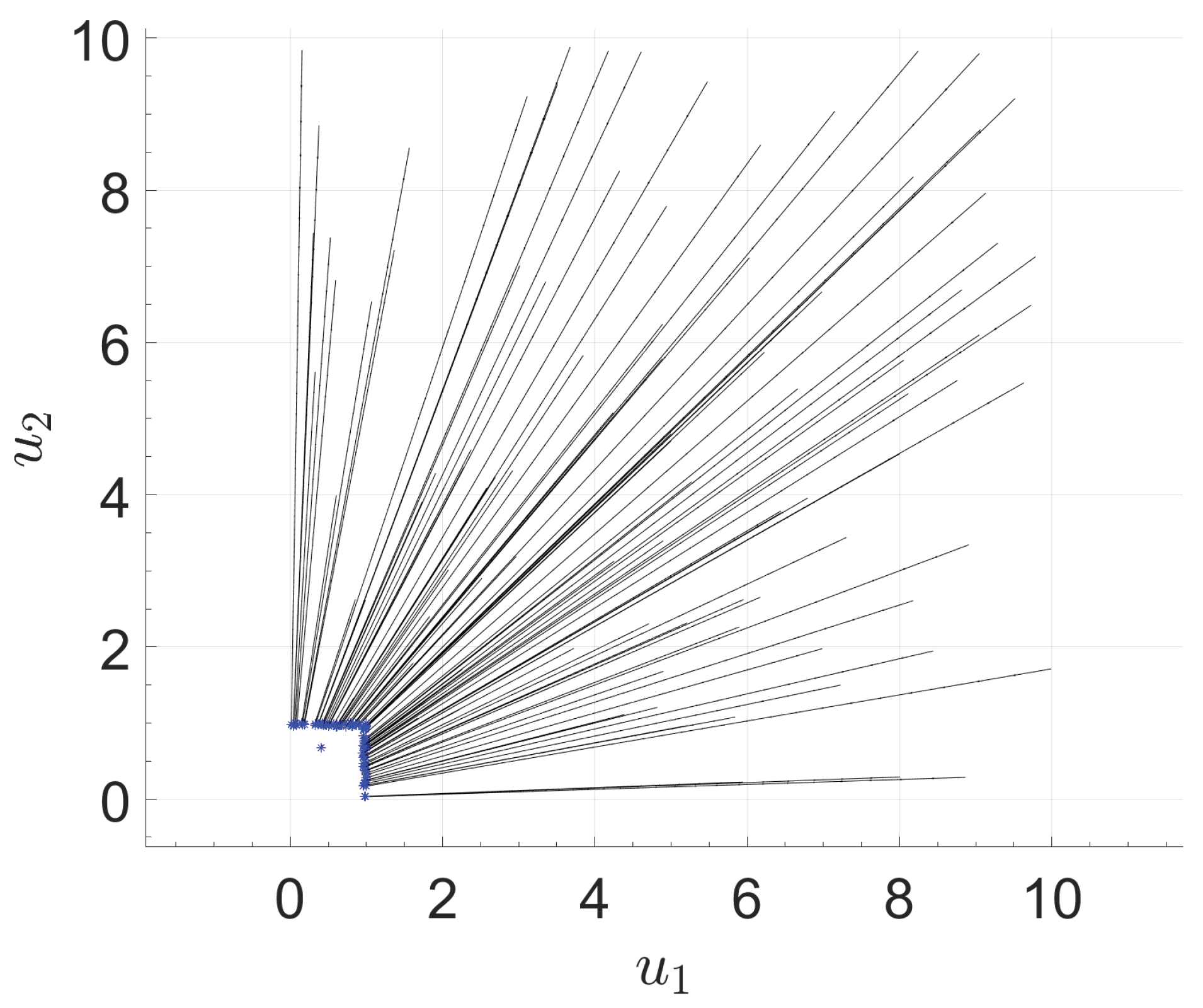

Table 1.
Sequence generated by Algorithm 1 for the problem (P1).
| 0 | 970 | |||
| 1 | ||||
| 2 | ||||
| 3 | ||||
| 4 | ||||
| 5 | ||||
| 6 | ||||
| 7 | ||||
| 8 | ||||
| 9 | 0 |
Table 2.
Sequence generated by Algorithm 1 for the problem (P2).
| 0 | 292 | |||
| 1 | ||||
| 2 | ||||
| 3 | 0 |
Table 3.
Sequence generated by Algorithm 1 for the problem (P3).
| 0 | 1 | |||
| 1 | ||||
| 2 | ||||
| 3 | ||||
| 4 | ||||
| 5 | ||||
| 6 | ||||
| 7 | ||||
| 8 | 1 | |||
| 9 | 1 | |||
| 10 | 1 | |||
| 11 | 1 | |||
| 12 | 1 | |||
| 13 | 1 | |||
| 14 | 1 | |||
| 15 | 1 | |||
| 16 | 1 | |||
| 17 | 1 |
Table 4.
The numerical results of Algorithm 1 for the problem (P4).
| Number of iterations | Computation times (in seconds) | |
|---|---|---|
| 100 | 4498 | |
| 120 | 4336 | |
| 140 | 4641 | |
| 160 | 4895 | |
| 180 | 4880 | |
| 200 | 4619 | |
| 220 | 4886 | |
| 240 | 4686 | |
| 260 | 4707 | |
| 280 | 5000 | |
| 300 | 5000 |
Disclaimer/Publisher’s Note: The statements, opinions and data contained in all publications are solely those of the individual author(s) and contributor(s) and not of MDPI and/or the editor(s). MDPI and/or the editor(s) disclaim responsibility for any injury to people or property resulting from any ideas, methods, instructions or products referred to in the content. |
© 2025 by the authors. Licensee MDPI, Basel, Switzerland. This article is an open access article distributed under the terms and conditions of the Creative Commons Attribution (CC BY) license (http://creativecommons.org/licenses/by/4.0/).
Copyright: This open access article is published under a Creative Commons CC BY 4.0 license, which permit the free download, distribution, and reuse, provided that the author and preprint are cited in any reuse.


