1. Introduction to DiD
With a DiD analysis we try to estimate whether a response variable (i.e. a variable exposed to a treatment) will achieve a mean value that, computed for the set of all treated units (treated group), is statistically different than the mean value computed for the set of some comparable untreated units (untreated or control group), once any factors affecting the link between the treatment and the effect (confounders) are ruled out. Therefore, the DiD analysis aims at “discovering” if a time contingent causal-effect relationship (post hoc, ergo propter hoc) between the response variable and the treatment is statistically consistent with the data. Examples of changes in response variables analysed with DiD after a treatment are numerous and encompass various research fields. They may be the human mortality rate, the unemployment, the quantity of corn harvested, to mention a few. The treatment or causal factor may include the use of a new pharmaceutical drug, the implementation of new training program for unemployed workers, the application of a new agricultural technique, etc. Other known examples of a response variable are SAT (Site Acceptance Test) scores of equipment under quality check, the level of pollution in a county before and after the adoption of environmental measures, or the tree cover density in a region subjected to reforestation. Thanks to its flexibility, DiD has been widely used in economics, public policy, health research, management and numerous other fields.
To purse the above causal analysis, DiD relies on a combination of before-after and treated-untreated group comparisons, but it is worth emphasising from the very beginning that the variable corresponding to the treatment must be expressed as a dichotomous variable (Zero vs One; Yes vs No) and not as a continuous variable. As it will be clarified later, treatment variables will play a role similar to the role played by dummy variables in traditional regression analysis. Not surprisingly, the term “treatment dummy” is frequently used in DiD studies or in studies that are structured as DiD models. The term dummy for example appears already in Ashenfelter & Card (1985) in their study of the effect of some training program in the USA where the longitudinal structure of earnings of trainees and comparisons group are used to estimate the effectiveness of the program for participants. In their study of the relationship between casual factor and response variable, Card & Krueger (1994) provide another early clear illustration of how the treatment is included in the analysis. They investigated whether an increase of minimum wage by New Jersey in 1992 from $4.25 to $5.05 (treatment) resulted in a statistically significant change in employment level amongst fast food restaurant workers in New Jersey (treated units) from that in neighbouring Pennsylvania, which did not change its minimum wage (untreated units). The treatment was not the amount of the wage increase (a possible continuous variable) but the “mere” asymmetric implementation (say, Yes in New Jersey and No in Pennsylvania) of the policy measure.
In general, the DiD analysis aims at estimating the mean difference between actual and potential realizations (the unobserved realizations of the response in the absence of the treatment) of a response variable in treated units after the occurrence of an asymmetric exogenous event (the treatment administered to treated units only) and uses instrumentally the actual response realizations recorded in untreated units. Yet, this modification of mean differences generally occurs over time, and the passage of time represents a complicating challenge in a DiD study. Whatever the response variable we study, the passage of time may affect in a potentially significant way the actual realization of the response as the data generation process proceeds through a possibly long-time span and encompasses several pre-treatment and post-treatment periods. Hence, the specific effect attributable to the passage of time (and the numerous factors potentially concealed in the passage of time) on the mean value of the response variable in both the control group and the treatment group must be properly considered. In other words, the researcher must determine if it was the treatment itself the cause of any change in the mean value of the response variable within the treatment group over and above what was caused by the pure passage of time or by time-conditioned factors. In summary, the main ingredients of the DiD approach to the estimation of the causal-effect relationship are the existence of a treatment administered to treated units only, the behaviour of the treated and untreated response variables before and after the moment the treatment was implemented, and an appropriate consideration for the passage of time.
In this Review we will present the DiD estimation approach to the causal-effect relationship. We will try to highlight how with the DiD method the effect of the treatment can be estimated separately from the effect of the passage of time. To do so we will first present the simplest DiD framework in which the treatment status of each unit can vary over time according to the following dynamics: an initial time period (e.g. months, years) in which there is no treatment is followed by a time period with treatment administered to some units only. The moment in which the treatment is introduced represents the temporal turning point of the entire period under examination. The units under investigation can in turn be assigned to two groups: those classified as never treated (the control group) because they are never subjected to the treatment during the entire sample period and those units that are treated in the post-intervention period only (the treated group). We will assume (section 1.1) that the latter are uninterruptedly treated from the introduction of the treatment until the end of the observed periods. In the initial simplest DiD framework we will assume that the treatment is the only relevant independent variable affecting the outcome of the response dependent variable. Then, we will discuss the OLS way to estimate the effect of the treatment (section 2) as well as the identification problems related to the estimation process (section 1.4). We will call this initial framework Homogeneous case without cofactors. Homogeneity means that all the treated units will start to receive the treatment in the same moment. The presence of cofactors will be discussed later when the Homogeneous case with cofactors will be analysed in section 6. Analogously, the model structure in which treatments are administered in different periods to different treated units and never administered to some other units will be considered later in section 7 and it will be termed Heterogeneous Case (with or without cofactors). DiD techniques to be used under more complicated data structure (e.g. data generating clustering phenomenon or spatial-temporal relations) will be analysed in sections 8, 8.1, 8.2, and 8.3 at the end of the Review before the concluding section 9 which also contains important warnings and caveats. A final set of sections (section 10 and followings) surveys some applications taken from the literature and discusses methods and results.
A particular aspect of DiD on which we decided to focus is the exogeneity character of the treatment and the so-called parallel trend assumption (section 1.2). They represent fundamental elements of the method. As some of the papers discussed at the end of the Review will show clearly, in many cases DiD represents the statistical approach need to overcome the simultaneity and endogeneity difficulties inherent in many circumstances in more traditional OLS estimation techniques. Yet, this advantage of DiD over alternative techniques requires that some crucial assumptions about the data generation process are satisfied.
This Review will also review other aspects of the DiD methods that, in our opinion, are not sufficiently considered by DiD literature. In particular, in section 1.3 we discuss the Stable Unit Treatment Value Assumption (SUTVA) and show why DiD identification process requires that the treatment applied to one (or more) unit should not affect the outcome for other units. In other words, we discuss why the potential outcome of a generic unit in the analysed sample should not depend on the treatment status of some other units in the same sample or on the mechanism by which units are assigned to the control or treatment groups. We also pay special attention to the role that confounding factors have in DiD (section 5) and in sections 7, 7.1, 7.2, and 7.3 we analyse the most widespread methods proposed to estimate DiD when the sample period encompasses more than two periods and there is treatment heterogeneity. As anticipated above, complex data structure, such as data clustering and spatial-temporal dependence, that can affect the DiD estimation strategy, are discussed in sections 8, 8.1, 8.2, and 8.3.
Although this simple Review is conceived for applied economists, readers should keep in mind that DiD most attractive features are its (relative) simplicity and wide applicability. After all, to carry out a basic DiD study, we just require observations from a treated group and an untreated (comparison) group both before and after the intervention is enacted. Accordingly, in the last sections we discuss some papers that have applied DiD techniques in various research areas relevant in a public economics or public policy perspective. We stress that health care is not an area covered by this review because readers can access many several DiD studies that have been used to evaluate new policies and health programs. For example, in the USA dozens of studies have estimated the effects of expanded Medicaid eligibility through the Affordable Care Act (ACA). Following the Supreme Court ruling on the ACA, each State in the US choses whether to expand its threshold for Medicaid eligibility. This possibility created groups of treated states and comparison (untreated) States and enabled the application of DiD. These studies have informed ongoing policy debates in the US about the future of the ACA and the reader is referred to that literature (see Zeldow and Hatfield, 2021 for an introduction).
Finally, we stress that this Review covers the basic (almost intuitive) DiD techniques. There are other more advanced reviews (Callaway, 2021; Roth et. al., 2023, just to mention two papers) as well as chapter 5 of Angrist and Pischke (2009) and chapter 21 of Wooldridge (2010) that should be consulted by more advanced users.
We lastly stress that SW packages useful to implement basic and more advanced DiD methods can be found in the following websites (alphabetic order):
In the Appendix to the Review will include a few homemade ad hoc data sets to be used as examples of the DiD estimation techniques analysed in the Review and to conduct exercises.
1.1. A 2 × 2 (Two Groups and Two Periods) Homogenous DiD with No Cofactors
This Review presents a review of basic methods and recent developments introduced in the DiD literature in the last 30 years. Clearly, the fundamental notions of DiD could be assumed to be almost common knowledge and in theory they should not require a new basic review to be added to the many that already exists. Yet, since we want to offer a (may be incomplete, but) self-contained treatment of the subject we start with the basic framework need to identify a DiD model.
Assume that we have randomly drawn from an infinite population two samples of individuals (with or without the same numerousness of units), respectively denoted as G1 and G2. We call i an individual belonging to G1 and j an individual belonging to G2. Assume that the two periods under study are two years, each divided for expositional convenience in 12 months. We observe in each month of the first of the two years under study the realization of a random variable y representing the relevant variable under our investigation (income, unemployment, indebtedness, hours of work, rate of financial criminality, level of fever, etc.). For reasons that will become clear very shortly we call y the response variable. If is the realization of y for an individual i in G1 recorded during each month t = (1, …, 24), then is month t mean value of y generated by data of individuals belonging to G1 with N representing the total number of individuals in G1. Correspondingly, is month t mean value for group G2, generated by all j individuals of that group formed by M individuals. As a result, for each year we record 12 mean monthly values for each group. Altogether, we have 48 mean observations in the 2-groups × 2-years dataset.
We assume that the monthly evolution of
and
during the first 12 months is
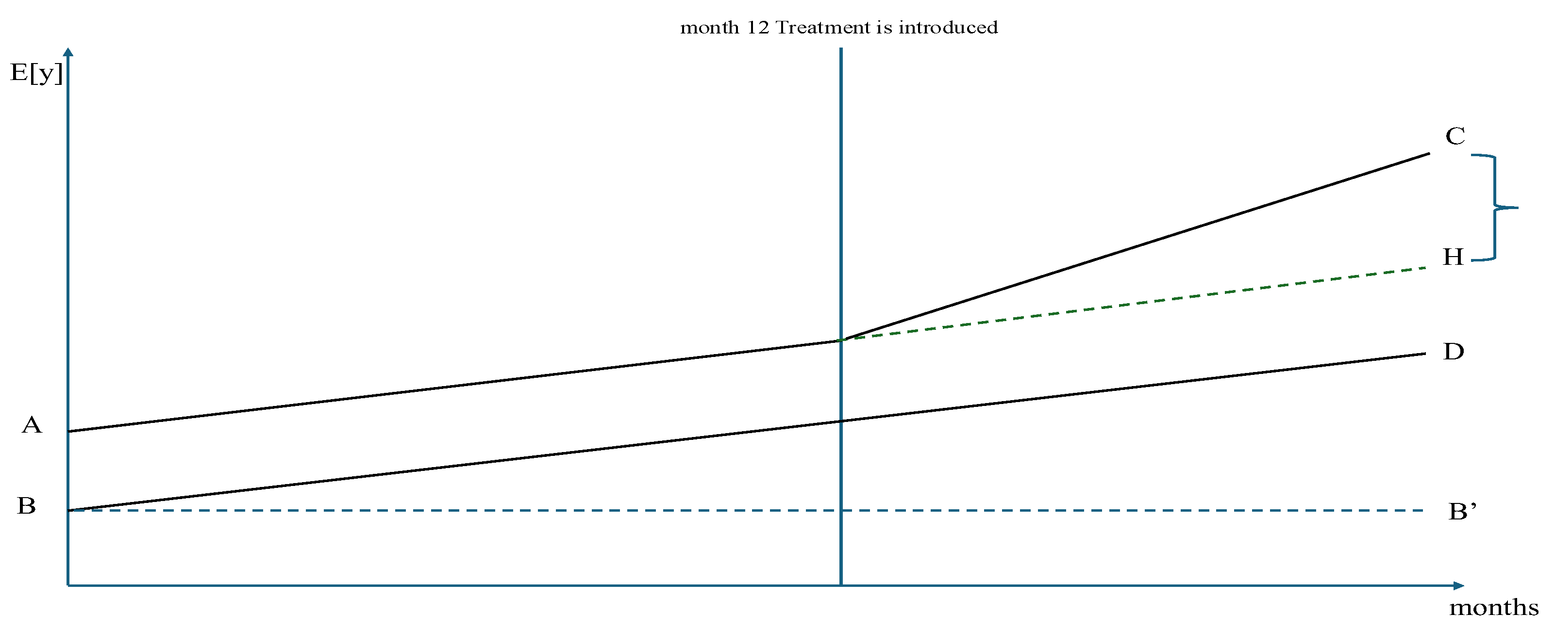
linearly parallel. In other words, we assume that the time evolution of the two series of mean values follows a parallel path having the same time slope so that the two paths are separated only by a group-specific constant (a sort of individual fixed effect used in the fixed effects least squares with dummy variables panel data analysis). Then, the plot of the time behaviour of the 24 mean values during the first year (first 12 months) corresponds to the left portion of
Figure 1 reproduced below (the first 12 months to the left of the vertical line).
Assume now that at the end of the first year (i.e. in correspondence to the vertical line in
Figure 1) “something” affecting
only G2 happened, ceteris paribus. That
something is generally assumed to correspond to an
exogenous event and it is called
Treatment (e.g. a new regulation, a more or less exogenous change of tax rates implemented in G2, some new subsidies paid to firms of that group, higher interest rates, a natural event, a new pharmaceutical therapy, etc.). This way of introducing Treatments should make clear that the word
“period” used in this DiD review is not synonymous of calendar unit of time but of “temporal phase”. In the 2 × 2 case we have two periods/phases: the first one (lasting 12 months) with no event and the second (lasting 12 months) with an event affecting the units of a group (G2 in our example) right from the
arrival of the event and continuously
until the end of our sample time.
We assume that individuals in G2
cannot anticipate the introduction of the treatment (and therefore cannot react in advance to its occurrence). Now it becomes relevant the right part of
Figure 1 (the part to the right of the vertical line). Inspection shows that the time path of the expected values of
y for the treated group G2 which, after the treatment, can be specified as:
(where Treatment = 1 means when the treatment is operative).
The G2 path has been twisted upward about the point in the plot corresponding to the last month of the first year (i.e. the last pre-treatment or pre-event month) while the time path of G1 proceeds according to the previous linear trend and is:
(where Treatment = 0 means when the treatment is not operative).
Hence, we assume that E[y] in G1 is unaffected by the treatment that is implemented with respect to G2 units only, and additionally that the treatment affecting G2 has no spillover effects on G1. Then, the dashed line represents the possible realizations of the expected values of the mean values of y for G2 in the absence of treatment but under the linear parallel trend hypothesis discussed above. In other words, the dashed line indicates what the path of the expected realizations of y in G2 would had been expected were the “perturbing” event (the treatment) absent, as if the Galilean inertia principle for uniform linear motion of corps was at work (no intervening external forces). Clearly, these realizations are not observed: actually, they do not exist. For that reason, we name them “potential realizations” as if they were the effect resulting from the application of a “vis inertiae, or force of inactivity” to use the terms employed by Newton in his Philosophiae Naturalis Principia Mathematica of 1687) because their force depends only upon their position (potential energy).
We now have all the ingredients useful to measure the
average effect that the treatment had on G2 (the treated group). The mean effect of the treatment is the difference between the value assumed by the mean
y in G2 after the treatment (solid line) and the value that it would had potentially assumed by pure
vis inertiae in the absence of the treatment (dashed line). That effect corresponds to the segment
CH in
Figure 1 whose length is the difference between the abscissa of point
C and the abscissa of point
H.
The measure of the length of the segment
CH =
C – H can be recovered as follows:
By manipulating the last equation, we express
CH as a
difference between two differences:
In the latter version, the measure of the treatment effect corresponds to the difference between two terms. The first term (included in the first parenthesis) measures
the difference in the realizations of the expected value of y for both groups (treated and untreated) in the post-treatment period, i.e. when
Treatment = 1 in the above expected values formulas. The second term (included in the second parenthesis) measures
the difference between the initial intercepts for the two groups i.e. when
Treatment = 0. The latter corresponds to the constant vertical distance of the two lines in the pre-treatment period and (under the hypothesis that the time trends are initially parallel and would had remained parallel in the absence of treatment). In other words, it is assumed that the constant initial difference (segment
AB) is constant during the entire period 1 because it depends only upon the above mentioned idiosyncratic constant elements and then, because of the Galilean inertia principle, it is bound to remain constant in the absence of treatment (the only new intervening force), even in period 2. This motivates the plot dashed line in period 2 in
Figure 1 and the previous description of those (unobserved) values as “potential”.
Therefore, the Average Effect of the Treatment upon Treated (ATET from now on) is obtained by differencing the mean response for the treatment and control units over time to eliminate time-invariant unobserved characteristics and also differencing the mean response of the groups (treated and untreated) to eliminate time-varying unobserved effects common to both groups. In other words, the DiD technique eliminates the influx of time-varying factors (confounders) by comparing the treatment group with a control group that is subjected to the same time-varying factors (confounders) as the treatment-receiving group.
As an example, we may think that y is the employment rate, and that the treatment is a subsidy paid only to firms in G2 (e.g. a particular area of the country) for every new employee. If expected unemployment in G1 and G2 follows a parallel trend in period 1 (when no subsidy was paid to firms), expected unemployment in G2 should stick to the linear trend of period 1 and remain parallel to that of G1. The dashed line would represent the potential expected value of unemployment in G2 in case of no subsidy granted to firms of G2 in period 2.
Figure 1 shows that the untreated group G1 has a role of paramount importance in the measurement procedure depicted above. G1 (untreated) acts as a
control group and supplies (loosely speaking) the substitutes for the unobservable (because they are never realised)
counterfactual observations of G2 to be used when studying the effect of the treatment. To be specific, the hypothesis is that in the absence of treatment reality would have evolved in G2 as described by the
E[
y] recorded in G1 with the obvious consequence that the right curly bracket in
Figure 1 would not exists because C → H. In other words, it would be
.
We can now proceed to estimate the effect of the event using all the expected values as follows.
C is the expected value of y for the treated group conditional upon the application of the treatment on that group
D is the expected value of y for the untreated group conditional upon the absence of the treatment for that group
A is the expected value of y for the treated group conditional upon the absence of the treatment
B is the expected value of y for the untreated group conditional upon the absence of the treatment
Therefore, calling
h = (
i, j) a generic individual in the
population (either treated or untreated, i.e. G1 + G2) we may write a linear regression model as follows
where:
yht is the value of the response variable for a unit in the population under study. Its value is measured in each group and each t, i.e. before and after the introduction of the treatment. It will correspond either to the i-th or to j-th observation at time t depending on the group (treated or untreated) of the unit.
β0 is the intercept of the regression model, common to treated and untreated units.
D1 is the Time Period Dummy which is a dummy variable that takes the value 0 or 1 depending on whether the h.th observation of the response variable refers to the pre (D1 = 0) or post treatment period (D1 = 1) independently on the group (treated or control) the observation belongs to. It simply indicates if that t is a period in which the treatment existed or not.
D2 is the Treatment Indicator Dummy which is a dummy variable that takes the value 0 or 1 depending on whether the h.th measurement refers to an individual in the control group (untreated) or in the treatment group respectively, independently on the time period. Therefore, D2 = 0 when the observation belongs to an untreated unit and D2 = 1 when the observation belongs to a treated unit (independently upon when the treatment was introduced). Clearly, in the simplified example of this section with only two periods, D2 = 0 means that the unit is never treated. Other settings are discussed in other sections.
D1× D2 is the interaction term between the time dummy and the treatment dummy. It s the most important coefficient to estimate. It measures the average effect of the treatment on treated units the estimated average differential impact of the treatment.
As it will be commented below, the above equation (1) represents the basic but elegant form of a DiD analysis for the homogenous case with no cofactors. In
Table 1 we analytically discuss the relevance of each coefficient. Here we stress that the
elegance of DiD (Goodman-Bacon, 2021 p. 254) makes it clear which comparisons generate the estimates, what leads to bias, and how to test the design. The expression in terms of sample means connects the regression to potential outcomes and shows that, under common trends assumption, a two-group/two-period (2×2) DiD identifies the average treatment effect on the treated.
The estimated coefficients of equation (1) have definite relations with the critical points of
Figure 1. These relations are illustrated in the following 2 × 2
Table 1 which gives a more explicit description of how the states of the word (time and treatment) can combine and how they affect the realization of
y in the above equation (1).
In what follows, the estimated coefficients obtained from an OLS regression of the model correspond to the expected values presented above. For the fitted model, the corresponding expectations are as follows. The caps (^) above the coefficients indicate that they are the estimated (fitted) values of the corresponding coefficients. Replacing
yht with the expected value of
yht also allows us to drop the error term
since by hypotheses in a well-behaved OLS regression model, the expected value of the error term is a zero mean and constant variance term. Hence, we can rewrite the content of each cell of the 2 × 2 matrix of
Table 1 as follows.
In terms of the hypothetical data set generating
Figure 1,
corresponds to point
B and must be interpreted as the average baseline common to the two groups (constant).
In terms of the hypothetical data generating
Figure 1,
still corresponds to point
B and, as above, and must be interpreted as the model baseline average (constant).
, which corresponds to slope of segment
DB, and is the time trend in control group in treatment.
In terms of the hypothetical data generating
Figure 1, we have that
- (i)
corresponds to point B, as above, and must be interpreted as the model baseline average (constant) and
- (ii)
, which corresponds to segment AB, is the constant difference between the two groups before the treatment.
In terms of the hypothetical data generating
Figure 1, the sum
corresponds to point
C.
We now proceed to calculate the difference in the expected value of y between the before (pre-) and after (post-) treatment phases of the study.
For the treatment group, the difference in expectations works out as follows:
which is the difference in estimated response between the after-treatment and before-treatment phases of the study recorded within the treatment group.
Similarly, for the control group we have:
The above is the difference in estimated response within the control group between the after-treatment and before-treatment phases of the study.
The
difference between the two differences measures the average net effect of the treatment on the treated group, that is,
The estimated coefficient is what we have called ATET (Average Treatment Effect upon Treated) and it has been obtained from the estimates of a linear model in which there a no cofactors (other independent variables affecting y). Its difference with respect to the similar measure of the treatment called ATE is discussed later.
For a more analytically grounded derivation of one may consult Angrist and Pischke (2009, p. 229) who discuss the expected DiD effect and then show the OLS regression that may be used for its estimation. Following the opposite route, Wooldridge (2010, p. 148) first starts from an OLS regression equation augmented with Treatment Dummies and then expresses and interprets the estimated relevant dummy as an estimate of the expected DiD treatment effect.
The following Remarks summarises the OLS use for a DiD strategy.
Remark n.1: the basic ingredients
We start with a set of i.i.d. individuals
i = 1, …,
n and a tuple
where
is the response variable,
is a cofactor vector (it may not be present) and
is the treatment assignment. We assume that the
potential outcome (realization of the response variable) depends on treatment and can be
We define the causal effect of the treatment as , the difference in potential outcomes of individual i, so that on average (population) we have that the Average Treatment Effect upon Treated (ATET) is . Clearly, each realization of the response can be observed in just one state of the word, i.e. conditional on either or , not both. Under the assumption that the treatment assignment is random (there is no systematic association between the potential outcome of an individual and the treatment), OLS methods can help us to overcome this missing data problem.
Remark n.2: ATET and OLS estimator
The OLS method of estimation of equation (1) correctly identifies the ATET in a DiD regression under parallel trend and no anticipation effects for it allows us to define the estimand which involves unobservable counterfactuals in a form (equation 1) that depends only on observed outcomes. This process is called “identification” (see below for more discussion).
Then, ATET is the expected value of the DiD effect between the treatment and control group (i.e.
CH in
Figure 1). After the DiD model is estimated, the estimated coefficient of the interaction term (
D1 ×
D2), i.e.
, will give us the estimated difference-in-differences effect of the treatment that we are seeking. The coefficient’s
t-score and corresponding
p-value will tell us whether the effect is statistically significant and if so, we can construct the 95% or 99% confidence intervals around the estimated coefficient using the coefficient’s standard error reported by the model output.
Finally, recall that we have randomly selected the participants (treated) and the non-participants (untreated). Therefore, at this stage we do not pose ourselves the question: why didn’t the non-participants participate? As we shall see, this question is outside the realm of DiD analysis. The general DiD assumption is that there is a sort of powerful external force determining in a random way the correct random sampling.
1.2. Violations of the Parallel Trend Assumption
Remark n.1 and
Figure 1 clearly indicate that the parallel trend assumption is one fundamental ingredient of DiD. Yet, the presence of parallel trends should not be ascertained from simple optical observation of plots like
Figure 1. There may be cases in which the pre-treatment trends of the treatment and control groups may appear different and the power to detect violations of parallel trends hypothesis is low. Or it may be the case that the pre-treatment trends were the same, but we have a reason to think that some other shock in the economy different than the treatment may cause the post-treatment trends to differ. Then, the question is: can we still use DiD when we are unsure about the validity of the parallel trends assumption? Rambachan and Roth (2023) note that one may assume that the pre-existing difference in trends persists from pre to post treatment periods and simply extrapolate this out. For example, we might assume that a difference in trends of 1% per month in the employment rate data set in treated and untreated areas would continue to hold after the treatment (say a policy wage intervention). Then, if the control group (no intervention) has employment grow at 3% per month after the intervention is passed, we would assume the treated group employment would have grown at 4% per month and compare the actual employment rate to this theoretical counterfactual. However, assuming the pre-treatment difference in trends carries out exactly in the post-treatment period is a very strong assumption, particularly if we did not have many pre-treatment periods over which to observe it. Rambachan and Roth (2023) suggest that researchers may instead want to consider robustness to some degree of deviation from the pre-existing trend, so that linear extrapolation need only be “approximately” correct, instead of exactly correct. This difference is realized by allowing the trend to deviate non-linearly from the pre-existing path by an amount, call it M –the bigger that amount, the more deviation from pre-existing trend is allowed. Once one abstains from imposing that the parallel trends assumption holds exactly, the (pseudo)parallel trend is tested by testing the restrictions on the possible post-treatment differences in trends (the above M) given the point identified pre-trends estimate. Such restrictions formalize the intuition motivating pre-trends tests, namely that pre-trends are informative about counterfactual post-treatment differences in trends. Then their paper shows that given M, we can identify a confidence set for the treatment parameter of interest. In doing so we clearly violate the “pure” parallel trend assumption needed to identify the DiD parameters and instead resort to a sort of partial identification approach. Researchers can then also find and report the breakdown point – how much of a deviation from the pre-existing difference in trends is needed before we can no longer reject the null. As an example, Rambachan and Roth (2023) consider the impact of a teacher collective bargaining reform on employment, in which parallel trends seem to hold for males, but in which there is a pre-existing negative trend for females. They show the DiD estimate for males at M=0 (linear extrapolation of the pre-existing trend), and then CI which get wider as they allow more and more of a deviation in trends (increasing M > 0). In contrast, for females, the DiD estimator is of opposite sign to what would be obtained when we extrapolate the pre-existing trend at M = 0, and then one sees how these results change as more deviations from these existing trends are allowed for.
Rambachan and Roth (2023) provide inference procedures that are uniformly valid so long as the difference in trends satisfies a variety of restrictions on the class of possible differences in trends and derive novel results on the power of these procedures. They recommend that applied researchers report robust confidence sets under economically motivated restrictions on parallel trends and conduct formal sensitivity analyses, in which they report confidence sets for the causal effect of interest under a variety of possible restrictions on the underlying trends. Such sensitivity analyses make transparent what assumptions are needed in order to draw particular conclusions.
A second approach is provided by Bilinski and Hatfield (2020). They recommend a move away from relying on traditional parallel trend pre-tests because of problems can emerge in both directions. Sometimes we may fail to reject parallel trends because the test power is low or, on the contrary, because the power is high. Yet, when we reject parallel trends, this doesn’t tell us much about the magnitude of the violation and whether it matters much for the results – with big enough samples, trivial differences in pre-trends will lead to rejection of parallel trends. Bilinski and Hatfield (2020) argue that the most popular approach to testing parallel trend is incorrect and frequently misleading and present test reformulations in a non-inferiority framework that rule out violations of model assumptions that exceed a threshold. We then focus on the parallel trends assumption, for which we propose a "one step up" method: 1) reporting treatment effect estimates from a model with a more complex trend difference than is believed to be the case and 2) testing that that the estimated treatment effect falls within a specified distance of the treatment effect from the simpler model. This reduces bias while also considering power, controlling mean-squared error. Our base model also aligns power to detect a treatment effect with power to rule out violations of parallel trends.
A third approach is proposed by Freyaldenhoven, Hansen and Shapiro (2019). Their idea is a solution similar to instrumental variables to net out the violation of parallel trends. For example, suppose that one wants to look at the impact of a minimum wage change on youth employment. The concern is that states may increase minimum wages during good times, so that labour demand will cause the trajectory of youth employment to differ between treated and control areas, even without the effect of minimum wages. Their solution is to find a covariate (e.g. adult employment) which is also affected by the confounder (labour demand), but which is not affected by the policy (i.e. if you believe minimum wages do not affect adult employment). Then this covariate can be used to reveal the dynamics of the confounding variable and adjust for it, giving the impact of the policy change. Importantly, this does NOT mean simply controlling for this covariate (which only works if the covariate is a very close proxy for the confounder of concern), but rather using it in a 2SLS or GMM estimator. Another example concerns the impact of SNAP program participation on household spending, where the main dataset has SNAP participation and the outcomes, and the concern is that income trends may determine both program participation and spending. Using a second dataset that has SNAP participation and income, they can instrument participation with leads of income, which requires assuming that households do not reduce labour supply in anticipation of getting the program.
1.3. The Stable Unit Treatment Value Assumption (SUTVA) (Rubin, 1978, I980, 1990)
DiD identification require that the treatment applied to one (or more) unit does not affect the outcome for other units. Following the definition of Angrist et al. (1996), Rubin (1980, 1990), Wooldridge (2010, 905) by Stable Unit Treatment Value Assumption (SUTVA) in causal studies we mean that the potential outcome for a generic unit does not depend on the treatment status of the other units or on the mechanism by which units are assigned to the control and treatment groups. In other words, treated and untreated units are expected not to mutually interfere and do not influence their outcomes (Cox, 1958). The authors themselves point out that the assumption is critical and does not always match with real situations. For instance, let us consider a generic market in which operators mutually know and interact, thus influencing the reactions to exogeneous or external events, or policies in which “spillover effects” among neighbours can affect the choices of people involved in the experiment (Sobel, 2006). Similarly, one could consider panel data settings in which units interact across temporal (e.g., anticipation effects), cross-sectional (Xu, 2024), and spatial dimensions (Wang, 2021; Wang et al., 2020; Xu, 2024). Imbens and Rubin (2015, pp. 10) use the example of the fertilizer applied to one plot that affected the yields in contiguous untreated plots. Another example might be that of students assigned to attend a tutoring program to improve their grades (treated units) who might interact with other students in their school who were not assigned to the tutoring program (untreated control units) and influence the grades of the latter. Treated students might affect “informally” the performance of the control students since their interaction can generate spillover effects of the treatment in favour of untreated students. Under these circumstances, to enable causal inference, the analysis might be completed at the school level rather than the individual level. SUTVA would then require no interference across schools, a more plausible assumption than no interference across students.
Hence, SUTVA demands that the potential outcomes for some untreated unit do not vary with the treatments assigned to some other treated units. In other words, a subject’s potential outcome is not affected by other subjects’ exposure to the treatment. The SUTVA implies that each individual has one and only one potential outcome under each exposure condition, that is with and without treatment (Schwartz et al., 2012), thus making the causal effect “stable”. On the contrary, when the SUTVA is not fulfilled, there could exist multiple potential outcomes for each individual under each exposure condition (i.e., the causal effect is not unique), potentially leading to lead to misleading inferences. In non-economic frameworks, researchers often add a second aspect of stability in causal studies and closely related to the original SUTVA, that is, the so called “consistency assumption” (Cole and Frangakis, 2009; VanderWeele, 2009) or “no-multiple-versions-of-treatment assumption”, which states that potential outcomes of individuals exposed to the treatment coincide with their observed outcomes. In other words, there are no hidden forms of treatment leading to different potential outcomes (Cerqua et al., 2022; 2023).
Laffers and Mellace (2020) introduced a third source of violation of the SUTVA, that is, the presence of measurement errors in either the observed outcome or the treatment indicator. While this new perspective extends the definition of the SUTVA, the authors also propose a way to relax the assumption by means of a sensitivity study. Specifically, they suggest computing the maximum share of units for which SUTVA can be violated without changing the conclusion about the sign of the treatment effect. According to the specificities of the empirical setting of interest, several other attempts to extend and to relax the SUTVA can be found in the recent literature (see, for instance, the paper by Qiu and Tong, 2021; VanderWeele et al., 2015 for a recent review on causal inference in the presence of interference). For instance, considering the case when all units are affected by the treatment, Cerqua et al. (2022) make use of a machine learning counterfactual framework in which the no-interference part of the SUTVA is substituted by a milder definition only requiring that the potential outcomes for treated units are not affected by the individual characteristics of the other treated units. Indeed, in Cerqua et al. (2023), the authors remove entirely the no-interference assumption and rely solely on the no-multiple-versions-of-treatment assumption, as they are aware that in many socio-economic applications agents are sensibly affected by interference across both space and time. Other strategies attempt to relax the assumption by using clustered or hierarchical data structures (for instance, individuals living restricted areas such as neighbourhoods) with potential spatial spillovers. VanderWeele (2010), for instance, introduced the definition of individual-and-neighbourhood-level SUTVA and neighbourhood-level SUTVA to deal with empirical setting in which cluster-level interventions are considered. Among others, Huber and Steinmayr (2021) allow for the interaction between individuals and higher-level structures (e.g., regions) and suggest a non-parametric modelling to separate individual-level treatment effects from spillover effects. However, while the SUTVA may be violated on the individual level, it must hold at the aggregate level. The latter can be referred to the regional SUTVA, which admits spillover effects between individuals within regions, but rules out spillovers across regions. Under this new setting, the total treatment effect may be split up into an individual effect and a within-region spillover effect driven by the treatment of other individuals in the region. Eventually, Ogburn et al. (2020) and Ogburn et al. (2024) considered the potential spillover effect produced by a network in which individuals mutually interact and treated individuals may spread the treatment to their social contacts.
In the rest of the Review, we will adopt the definition of SUTVA provided in Remark n.2, that is,
Remark n.3: the SUTVA assumption
The potential outcomes for any unit do not vary with the treatments assigned to other units, and, for each unit, there are no different forms or versions of each treatment level, which lead to different potential outcomes.
Essentially, Remark 3 states that an individual’s potential outcome under a given treatment depends neither on the treatment received by other individuals nor on different versions of the treatment itself. In other words, each individual has only one potential outcome for each level of treatment, and this outcome is independent of the treatment received by others. Specifically, we must make sure (i) that an individual’s outcome is not influenced by the treatment received by other individuals. For example, if we are evaluating the effect of a drug, SUTVA implies that whether a patient takes the drug does not affect the outcome of another patient who might not take it and (ii) that for each level of treatment, there is a unique version of the treatment that leads to a given potential outcome. This means that there are no different versions of the treatment that could lead to different outcomes for the same individual.
We may conclude that SUTVA is crucial for the correct interpretation of causal effects because, if violated, it can lead to biased estimates of treatment effects. For example, if interference is present (a student treated with a new textbook shares the improvements of her/his knowledge with an untreated fellow student), we may not be able to distinguish the effect of the treatment from the effect of the interactions between treated and untreated individuals.
1.4. Exogeneity and Identification. DiD and Traditional Econometrics
In OLS regression analysis we are interested in assessing the effect of a (usually) continuous variable
x on a dependent
Y under the hypothesis of exogeneity. The “true” causal effect of
x on
Y can be identified as long as independent changes of
x only produce a direct effect on
Y, by ruling out any potential indirect effect of
x on
Y occurring via the relation of
x with unobservable factors. Without this exogeneity condition, OLS produced biased estimated parameters. Using Cerulli’s (2015) example, we assume that the regression model is
where
β represents the causal effect of
x on
Y and
u is a non-observable factor. By differentiation we have
The model is identified as long as . If the autonomous changes in x are not exogenously determined, as x has also an indirect effect on Y through its effect on u and since u is not observed we cannot separate the direct effect (β) and the indirect effect ( and the model is no longer identified.
The counterfactual approach of the DiD to causality can be reformulated in terms of OLS model with the x assuming a binary form (say x0 for the treated and x1 for the untreated) instead of a continuous x. If we can observe two responses (Y0 state: treatment and Y1 state: no treatment) we write
Subtracting the second equation from the first we have
If a bias similar to the previous one is generated even when we use binary form data typically associated with treatment events and counterfactuals. Exogeneity of treatment is a necessary condition.
In DiD analysis we may go a little further and portrait the identification problem using the assumptions made above in section 1.1. We can re-write the target estimand of section 1.1 (which involved unobserved counterfactuals) in a form that depends only on observed outcomes. In DiD we call this process “identification”. To do so we assume that
the change in response from pre- to post-intervention in the control group is a good proxy for the counterfactual change in untreated potential outcomes in the treated group. When in a 2 periods framework we observe the treated and control units only once before treatment (
t = 1) and once after treatment (
t = 2), we write this as:
Notice that it involves unobserved counterfactual outcomes, namely
(the potential realization of y in case of no treatment; recall from
Figure 1 that these data no not exist). This is other way to state the parallel trend assumption or the
counterfactual assumption.
We also need to make more explicit another assumption of section 1.1. For DiD the treatment status of a unit can vary over time. However, we only permit two treatment histories: never treated (the control group) and treated in the post-intervention period only (the treated group). Thus, we will use D = 0 and D = 1 to represent the control and treated groups, with the understanding that the treated group only receives treatment whenever
T > T
0. Every unit has two potential outcomes, but we only observe one — the one corresponding to their actual treatment status.
The consistency assumption links the potential outcomes
at time
t with treatment d with treatment
d ∈ D = (0,1) to the observed outcomes
:
Finally, we add the assumption that future treatment does not affect past outcomes. Thus, in the pre-intervention period, the potential outcome with (future) treatment and the potential outcome with no (future) treatment are the same (no anticipation effects).
Using the assumptions made above, we can re-write the target estimand (which involved unobserved counterfactuals) in a form that depends only on observed outcomes. In DiD this process is specifically called “identification” and should not be confused with the specification problems typical of traditional OLS single equation regressions or with the so called over or under identification problems emerging from multi equations OLS systems. DiD identification relies on the Counterfactual Assumption and the Consistency Assumption discussed above, and ends with the familiar DiD estimator where for reducing notation we use
D instead of
D2 of equation (1) and indicate periods as numbers between parenthesis (see Callaway, 2022, 8):
You may compare the above ATET with the result obtained in section 1.1. To simplify reading and comparison we summarise the meaning of the above terms as follows:
is the post-intervention average response of the treated group
is the pre-intervention average response of the treated group
is the post-intervention average response of the control group
is the pre-intervention average response of the control group
In summary, DiD identification begins with the ATET, applies the Counterfactual Assumption and the Consistency Assumption, and ends with the familiar DiD estimator.
In section 3 we present a worked example in which the above expected values are computed and used to calculate the ATET coefficient as a difference among differences.
When we observe the treated and control units multiple times before and after treatment, we must adapt the target estimand and identifying assumptions accordingly. Identification problems with multi period DiD is discussed later.
Appendix A provides an example with an easy visualization of the data set
2. The OLS Version of the Two-Way Fixed Effects Regression (TWFE)
TWFE is the most common way to implement a DiD identification strategy under the assumption of treatment homogeneity. In this section we present what Roth, Sant’Anna, Bilinski, and Poe (2023, p. 2224) call a “static” TWFE which regresses the outcome variable on individual and period fixed effects and an indicator for whether the unit
h is treated in period
t. Recall that in section 1.2 we have defined
Then, the estimated ATET can be written by
replacing population means by their sample analogues (indicated by upper bars) to obtain
The above expression is algebraically equivalent to either of the following OLS regression system
where in the system
i indicates treated units,
j indicates untreated units, and
t is time, and
h in equation (2) below can be either
i or
j. The interpretation of the quantities involved in (2) is the following:
is the response variable
is a time effect
is a unit (not group) fixed effect
is the dummy (indicator) for whether or not unit h is affected by the treatment in period
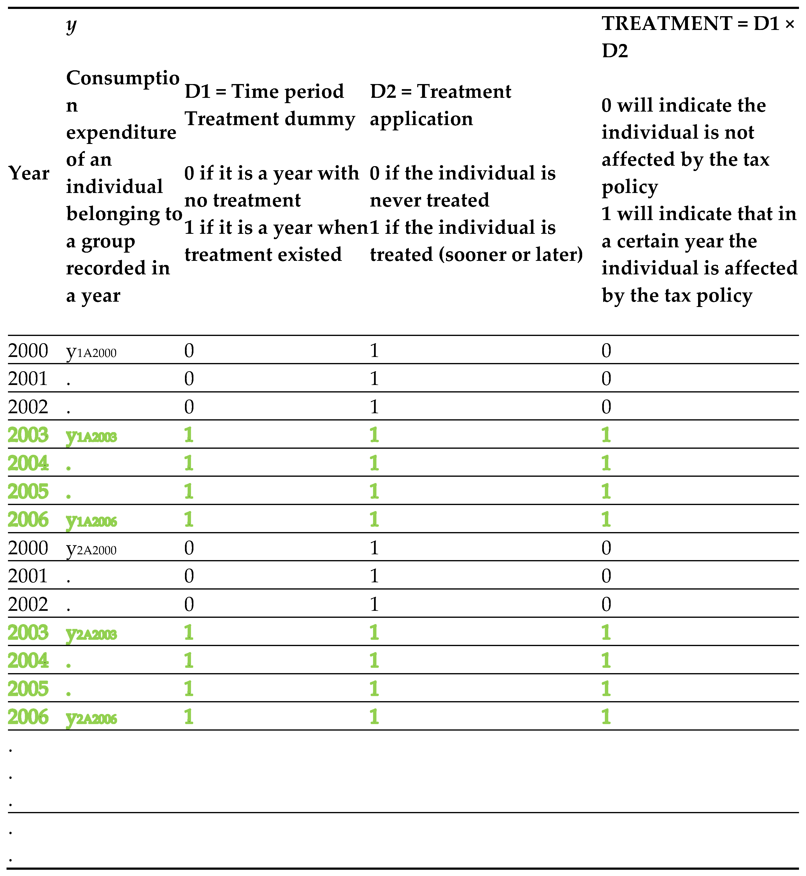
t (the term D1 × D2 of the last column of
Table 2)
are idiosyncratic, time-varying unobservable factors.
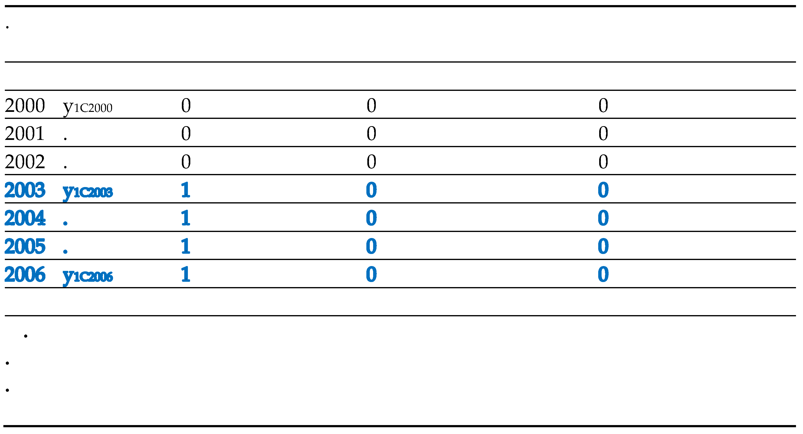
Table 2.
Example of data set for DiD with more than two years.
Table 2.
Example of data set for DiD with more than two years.
Table 2a.
Example of a DiD data set.
Table 2a.
Example of a DiD data set.
| 1 |
1 |
0 |
.5 |
| 1 |
2 |
0 |
.5 |
| 1 |
3 |
0 |
.5 |
| 1 |
4 |
0 |
.5 |
| 1 |
5 |
0 |
.5 |
| 1 |
6 |
0 |
.5 |
| 1 |
7 |
0 |
.5 |
| 1 |
8 |
0 |
.5 |
| 1 |
9 |
0 |
.5 |
| 1 |
10 |
0 |
.5 |
| 2 |
1 |
0 |
1 |
| 2 |
2 |
0 |
1 |
| 2 |
3 |
0 |
1 |
| 2 |
4 |
0 |
1 |
| 2 |
5 |
1 |
2 |
| 2 |
6 |
1 |
2 |
| 2 |
7 |
1 |
2 |
| 2 |
8 |
1 |
2 |
| 2 |
9 |
1 |
2 |
| 2 |
10 |
1 |
2 |
| 3 |
1 |
0 |
2 |
| 3 |
2 |
0 |
2 |
| 3 |
3 |
0 |
2 |
| 3 |
4 |
0 |
2 |
| 3 |
5 |
1 |
4 |
| 3 |
6 |
1 |
4 |
| 3 |
7 |
1 |
4 |
| 3 |
8 |
1 |
4 |
| 3 |
9 |
1 |
4 |
| 3 |
10 |
1 |
4 |
Table 2b.
Data set of a worked example.
Table 2b.
Data set of a worked example.
| Consumers’ Id |
Time |
Consumption € |
D1 |
D2 |
| 1 |
2010 |
12 |
0 |
1 |
| 2 |
2010 |
9 |
0 |
1 |
| 3 |
2010 |
13 |
0 |
1 |
| 4 |
2010 |
14 |
0 |
1 |
| 5 |
2010 |
15 |
0 |
1 |
| 6 |
2010 |
13 |
0 |
0 |
| 7 |
2010 |
14 |
0 |
0 |
| 8 |
2010 |
13 |
0 |
0 |
| 9 |
2010 |
16 |
0 |
0 |
| 10 |
2010 |
15 |
0 |
0 |
| 1 |
2011 |
15 |
1 |
1 |
| 2 |
2011 |
17 |
1 |
1 |
| 3 |
2011 |
19 |
1 |
1 |
| 4 |
2011 |
18 |
1 |
1 |
| 5 |
2011 |
22 |
1 |
1 |
| 6 |
2011 |
13.5 |
1 |
0 |
| 7 |
2011 |
14 |
1 |
0 |
| 8 |
2011 |
15 |
1 |
0 |
| 9 |
2011 |
15.5 |
1 |
0 |
| 10 |
2011 |
14.4 |
1 |
0 |
Equivalently, the previous system can be written in a single equation (panel data) version as follows:
where
is the individuals fixed effect,
is the time fixed effect, and
is the treatment dummy interaction. We can estimate equation (2) and interpret the estimated coefficients according to the result reported in Remark n.4 below, that is,
Remark n.4: causal interpretation of the TWFE estimator
Under parallel trend, treatment homogeneity and no spill-over, is the TWFE estimation of the causal effect of receiving the treatment.
As the very name suggests TWFE is the case where there are exactly two time periods, where no units is treated in the first time period, and where some units become treated in the second time period while other units remain untreated in the second time period. Notice that when we say periods we do not necessarily refer to units of time (years, months etc.) but to “time intervals”: the first (possibly composed by several years, several months, etc.) in which there is no treatment for nobody and the second (possibly composed by several years, several months, etc.) in which some units are treated (uniformly).
To illustrate formally TWFE we need some notation. Let us define the following quantities:
Then for
define
yht(1) to be unit i’s potential treated response in period
t and correspondingly
yht(0) to be unit i’s potential untreated response in period
t. Impose that
for all units. This is the no anticipation condition of section 1. It states that the treatment should not affect the response variable in periods before the treatment takes place. The result from the above assumption and conditions is that
In the first time period we observe untreated potential outcomes for the response variable for all units and in the second period we observe treated potential outcomes of the response variable for treated units and untreated potential outcomes of the response variable for untreated units.
Using the above definitions, we may define the ATET resulting from the DiD identification of the treatment effect as follows
which is equivalent to the one given in the previous section.
Using Callaway’s (2022, p. 6) definition, the ATET is the mean difference between treated and untreated potential outcomes among the treated group. Perhaps a main reason that the DID literature most often considers identifying the ATET rather than, say, the average effect of treatment is that, for the treated group, the researcher observes untreated potential outcomes (in pre-treatment time periods) and treated potential outcomes (in post-treatment time periods). The DID identification strategies exploit the above framework. As a result, it is natural to identify causal effect parameters that are local to the treated group.
Clearly, the model presented in equation (2) is the static specification of the TWFE, which yields a sensible estimand when there is no heterogeneity in treatment effects across either time or units. Following Roth, Sant’Anna, Bilinski, and Poe (2023, p. 2224) we can stress the relevance of these hypotheses more formally.
Define a period (e.g. year) g > t and let τh,t (g) = Yh,t(g) – Yh,t(∞). Suppose that for all units h, τh,t(g) = τ whenever t ≥ g. This implies that (a) all units have the same treatment effect, and (b) the treatment has the same effect regardless of how long it has been since treatment started. Then, under a suitable generalization of the parallel trends assumption and no anticipation assumption, the population regression coefficient α in equation (2) is equal to τ.
Yet, issues arise, however, when there is heterogeneity of treatment effects over time, as shown in Borusyak and Jaravel (2018), de Chaisemartin and D’Haultfoeuille (2020), and Goodman-Bacon (2021), among others. More generally, if treatment effects vary across both time and units, then τh,t(g) may get negative weight in the TWFE estimand for some combinations of t and g.
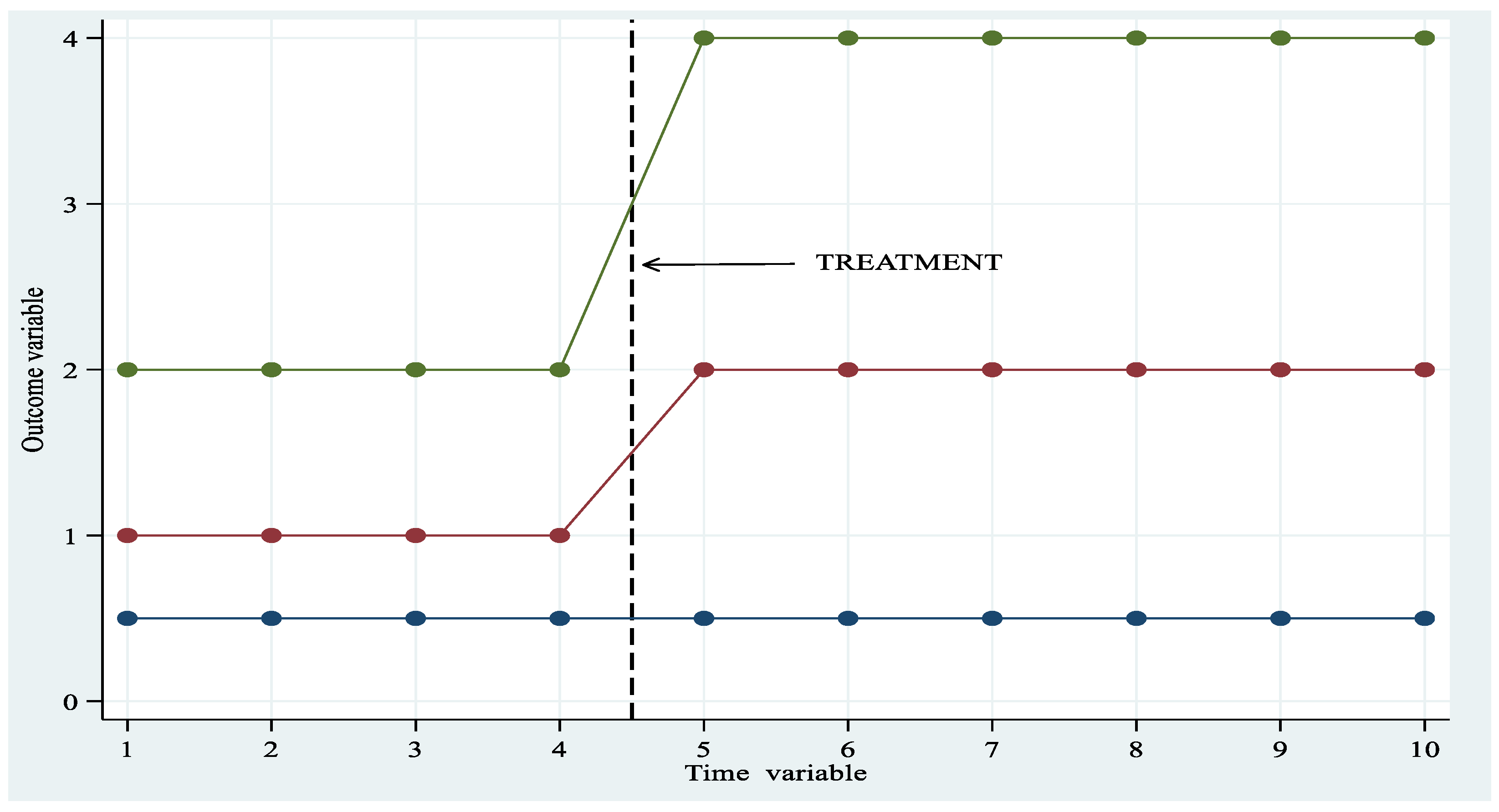
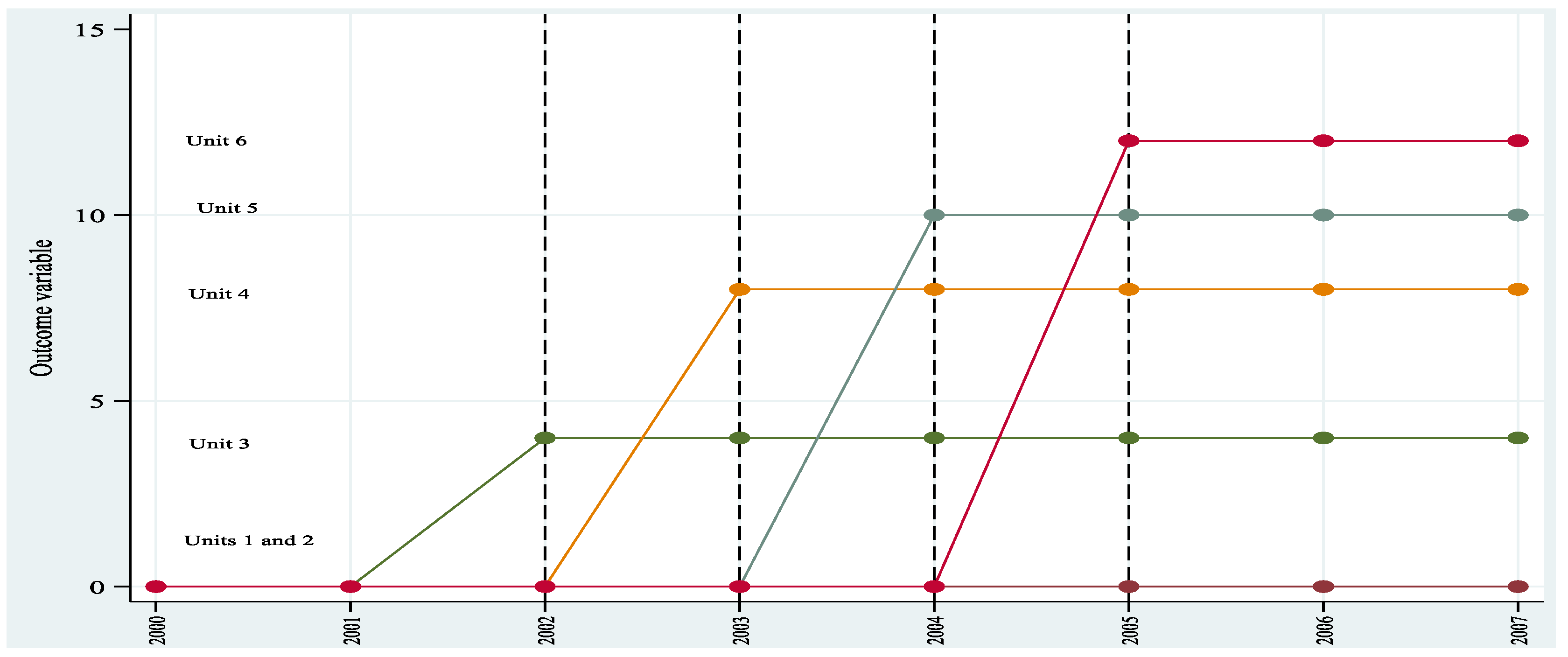
Figure 2 gives the idea of parallel trend with 3 units (unit 1 blue colour is untreated) and 10 periods. The plot has been generated using the data of
Table 2a reported in the Appendix. The following plot illustrates the time paths of the response variable. Notice that Unit 1 is never treated; Units 2 and Unit 3 start treatment at time 5 and are always treated from t = 5 to t =10.
2.1. Testing for the Parallel Trends and Anticipation Effects Assumptions in the TWFE Model
Given the fundamental importance of the parallel trend assumption, a natural question is: how to test for parallel trends in a panel data TWFE? In order to find answers, we start from the above model written as
where
is the indicator function, the treatment is indexed by
Dh, whit
Dh = 1 indicating that observation
h is part of the treated groups/units and
Dh = 0 indicates that it is part of the comparison/control group. Let
t index time from {1, ..., T} and suppose that an intervention begins at time
T0 for the treated units (same treatment periods for all treated units: the so-called homogenous case. See below). All other symbols have their usual meaning. The treatment effects of interest are
βk, representing differential post-period changes in the treated group relative to comparison at each time point. The average of these coefficients, that is,
is the average ATET.
We may exploit the above definition of the coefficients to derive some tests of the DiD identification hypothesis.
Parallel trends test: the slope test. In a parallel trends test for DiD identification, we may try and estimate whether there is a difference in slope between treatment and comparison groups prior to the intervention. Call
θ the different coefficient. Then, rewrite the above equation in a form that incorporates the pre-treatment coefficient
θ:
We can now test whether the (pre-treatment) differential slope θ = 0. If the null hypothesis for this test is non rejected (i.e., pv > 0.05), researchers may conclude that trends are parallel.
Anticipation effects: Researchers may instead examine the validity of the identification of the parameter by DiD by testing whether there is a significant “treatment” effect prior to the intervention, that is. an effect starting at T* < T
0. In this context, they might use the modified original panel model:
and estimate it by omitting data from after T
0. If the test statistic
is significant, this again suggests a violation of parallel trends. (Alternatively, a joint F-test can be used to test whether placebo effects at all possible
T* <
T0 were insignificant.)
2.2. More on the Parallel Trend Assumption
We have already stressed that DiD does not identify the treatment effect if treatment and control groups were on different trajectories prior to the treatment (common trend or parallel trend assumption).
With respect to equation (1) as the OLS equation of our DiD model we recall that
These assumptions guarantee that the common trends assumption is satisfied but they cannot be tested directly. This is quite disappointing because it leaves the tests for parallel trend the optical ability to visual checking on trends reported in plots.
In
Figure 1, we illustrated the case of an obvious pre-treatment parallel trend. In other cases, the assumption may be easily violated. Therefore, the question is: what has to be done? For those who think that hypothesis testing is in the realm of
optics and not
in the realm of mathematical statistics, a way to proceed is to inspect
visually the plot of the treated and untreated data.
Figure 1 is clearly a case of non-optically distorted test of parallel trend. The alternative presentation could be the make the G2 line start from A (eliminate the difference AB, which is the idiosyncratic constant element) and observe whether or not G1 and G2 lines overlap before the introduction of the treatment and diverge in period 2. More in general, optics cannot be a good substitute for mathematical statistics.
We may go back to initial 2 × 2 case and present a discussion of the parallel trend relevance. We had 2 groups, one treated and one untreated, and we indicate them as follows
where 0 is untreated (control) and 1 is treated. We also had 2 years and then we write
where 0 is the before treatment period and 1 is the treatment period. The guarantee a consistent estimate of the ATET we need to make the following parallel trend assumption
If the treated units had not received the treatment, the groups defined by
and
should have response variable showing the same paths as in
Figure 1 and
Figure 2. The group effects must be time invariant, and the time effect must be group invariant.
Within a 2-period framework, the possible “test” of this assumption is only graphical but for more than 2 periods same testing procedure based on Wald test are available. Many sw offer such statistical tests. We will present them alongside applications at the end of the Review.
In the linear case, Wooldridge (2021) has shown that tests of the Parallel Trend assumption are easily carried out in the context of pooled OLS estimation. In other words, in linear DiD models within a staggered treatment framework, the parallel trends assumption can be tested using pooled OLS estimation. This approach leverages the inclusion of cohort and time period dummies, along with cohort-by-time treatment indicators, in a linear regression model. The key idea is that under the parallel trends assumption, the coefficients on these interaction terms, when estimated via pooled OLS, are consistent for the estimation of ATET. Moreover, the tests are the same whether based only on the observations (imputation regression) or on pooled OLS using all observations— provided full flexibility is allowed in the treatment indicators. In other words, tests obtained pooling over the entire sample are equivalent to the commonly used ‘pre-trend’ tests (i.e. common tests used to examine the parallel trends assumption) that use only the untreated observations. As discussed by Wooldridge (2021), this means the tests using post-treatment data are not ‘contaminated’ by using treated observations—if the treatment effects are allowed to be flexible.
The algebraic equivalence of the pooled tests and pre-trends tests carries over to the nonlinear case provided the canonical link function is used in the Linear Exponential Function (LEF). In a DiD analysis with panel data, when using a linear exponential family (LEF) with the canonical link function, the pooled tests (using all data) and pre-trends tests (using only untreated observations) are algebraically equivalent. This means that the same underlying statistical properties and results can be obtained regardless of whether you pool all the data or focus only on the pre-treatment observations to check for parallel trends. Technically, if one uses a different mean function or different objective function, the test should be carried out using only the Dit = 0 observations (although it seems unlikely the difference would be important in practice). Wooldridge (2023) recently discusses the non-linear case.
In general, one should consider that the implications for applied work revolve around the (often-implausible) parallel trend assumption needed for the identification (using non-treated post treatment observations as counterfactuals) of a DiD model. Yet rather than just asserting that parallel trends hold, or abandoning projects where a pre-test rejects parallel trends (not to speak of the so-called optical test based the trend plots!), new approaches focus on thinking carefully about what sort of violations of parallel trends are plausible and examining robustness to these. Importantly, these methods should be used when there is reason to be sceptical of parallel trends ex ante, regardless of the outcome of a test of whether parallel trends hold pre-intervention. This type of sensitivity analysis will allow one to get bounds on likely treatment effects. For instance, a recent application comes from Manski and Pepper (2018), who look at how right-to-carry laws affect crime rates, obtaining bounds on the treatment effect under different assumptions about how much the change in crime rates in Virginia would have differed from those in Maryland in the absence of this policy change in Virginia.
In summary, the default DiD estimation equation should allow for a linear trend difference. This is a key recommendation of Bilinski and Hatfield (2020).
Which approach to use to examine robustness will depend on how many pre-periods you have: with only a small number of pre-intervention periods, the Rambachan and Roth approach of bounding seems most applicable for sensitivity analysis; when you have more periods you can consider fitting different pre-trends as in Bilinski and Hatfield (2020). Some issues are discussed in sections below.
3. Simple Worked Examples
We offer two simple numerical examples of ATET estimation with OLS and of the interpretation of the estimated coefficients. The second example relates to the interpretation of the response variable paths (before and after the treatment) as a tool for the evaluation of the presence of parallel trends.
3.1. Example n.1
Assume we have a total of 10 Consumers in 2 equal-sized groups (a group of 5 treated consumers and a group of 5 untreated consumers); 2 periods corresponding to two years, namely 2010 and 2011; a Treatment occurring at the end of 2010 (consumption tax reduction for the control group only). We name treated consumers Mrs. 1- 5; and untreated consumers: Mrs. 6 -10. Data and dummies are presented in
Table 2b in the Appendix.
Using the above dataset, we show by direct calculation of mean values how to recover the ATET induced by the treatment. We need the following quantities:
Estimated results can be synthesized in the following 2x2 matrix
| |
Control |
Treated |
| Pre-Treatment |
14.2 |
12.6 |
| Post-Treatment |
14.48 |
18.2 |
Therefore, we obtain the ATET as the difference of the two differences:
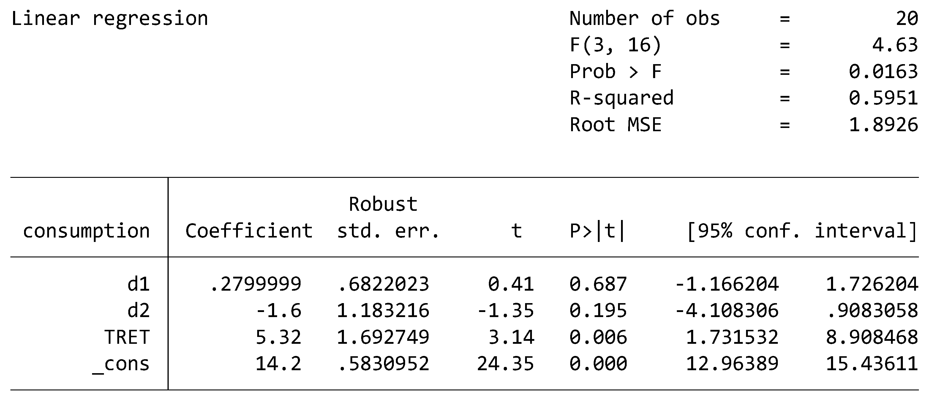
Clearly, the above calculation does not tell us how “good” the computed ATET is from an inferential point of view. In other words, 5.32 has no CI around it or P-values. That’s why we must re-obtain the result following a route that allows to introduce inferential elements. Now we estimate ATET with the OLS after the creation using the above defined D1, D2 and TRET = D1× D2. (reported in small letters in the Table below). We run the OLS (with the option of robust SE) regression of equation (1) and obtain the results reported below.
Then, the estimated ATET is 5.32, which, according to the t-test reported in the table, is statistically significant at any level. Recall that TRET is the D1×D2 dummy variable.
We can interpret the above estimated coefficients as it follows:
The estimated Constant = 14.2 (with a p-value smaller than 0.05) is the mean value of the Consumption in the control group in 2010 (i.e. before the treatment). We can compare it with the result obtained from the numerical calculation reported above. The two figures coincide.
If we sum the coefficient Constant and the d2 coefficient, i.e. if we calculate 14.2 + (– 1.6), we obtain 12.6. This is the expected Consumption of the control group in 2011, i.e. during the year of treatment.
If we sum the coefficient Constant and the d1 coefficient, i.e. if we calculate 14.2 + 0.28 = 14.48, we obtain the mean value of the Consumption in the treatment group in 2010, i.e. before the treatment.
The estimated TRET = 5.32 is the (statistically significant) treatment effect. Treated units increase their average consumption by 5.32 euros with respect to untreated individuals.
In formula, we may write, after indicating differences with the symbol Δ, the calculation of ATET as
As it was stressed above, equation (1) is estimated with OLS under the robust SE option, which allows adjusting the model-based standard errors using the empirical variability of the model residuals which are the difference between observed outcome and the outcome predicted by the statistical model. The motivation of this choice is that as shown by Bertrand, Duflo, and Mullainathan (2004) the standard errors for DiD estimates are inconsistent if they do not account for the serial correlation of the outcome of interest. For a more complete discussion, see Cameron and Miller (2015) and MacKinnon (2019) and the references therein.
Generalising our discussion beyond the 2-group example studied above, we may stress that the response variables under investigation usually vary at the group and time levels, and so it makes sense to correct for serial correlation. Bertrand, Duflo, and Mullainathan (2004) show that using cluster–robust standard errors at the group level where treatment occurs provides correct coverage in the presence of serial correlation when the number of groups is not too small. Bester, Conley, and Hansen (2011) further show that using cluster–robust standard errors and using critical values of a t distribution with G − 1 degrees of freedom, where G is the number of groups, is asymptotically valid for a fixed number of groups and a growing sample size. In other words, consistency does not require the number of groups to be arbitrarily large, that is, to grow asymptotically. Cluster–robust standard errors with G−1 degrees of freedom are the default standard errors in many sw performing DiD analysis.
Hence, we could still obtain reliable standard errors even when the number of groups is not large. But what about data with a very small number of groups? Cluster–robust standard errors may still have poor coverage when the number of groups is very small or when the number of treated groups is small relative to the number of control groups. For cases where the number of groups is small,
Stata sw provides three alternatives. In what follows I reproduce the description of the alternatives provided by Stata to deal with the issue (
https://www.stata.com/manuals/tedidintro.pdf.). The first alternative is to use the wild
cluster bootstrap that imposes the null hypothesis that the ATET is 0. Cameron, Gelbach, and Miller (2008) and MacKinnon and Webb (2018) show that the wild cluster bootstrap provides better inference than using cluster–robust standard errors with t(G − 1) critical values. The second alternative comes from Imbens and Kolesar´ (2016), who show that with a small number of groups, you may use
bias-corrected standard errors with the degrees of freedom adjustment proposed by Bell and McCaffrey (2002). For the third alternative, one may use
aggregation type methods like those proposed by Donald and Lang (2007); they show that their method works well when the number of groups is small but the number of individuals in each group is large.
When the disparity between treatment and control groups is large, for example, because there is only one treated group or because the group sizes vary greatly, cluster–robust standard errors and the other methods mentioned above underperform. Yet the bias-corrected and cluster–bootstrap methods provide an improvement over the cluster–robust standard errors.
3.2. Example n.2
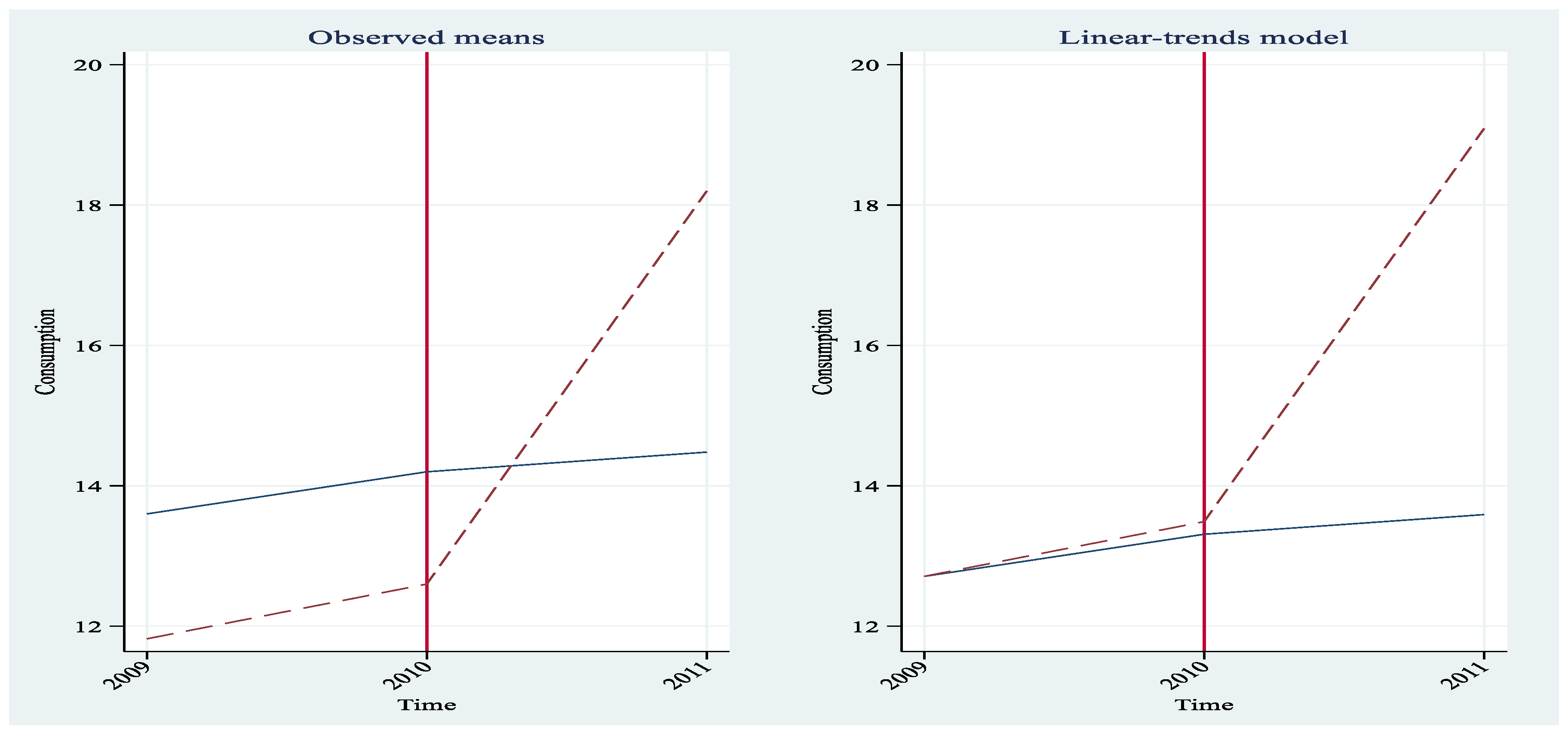
Use the data of
Table 3 in the Appendix (stuck in panel data form, i.e. in the version that is always recommended is defined by individual identity and time indicator) to generate a working data set for the future application of DiD. Answer the following “trivial” questions. How many units belong to the panel? By looking at D2, say how many units are treated Are the latter treated in the same years? What does D1 indicate? How is the dummy whose estimated coefficient corresponds to ATET obtained?
Assume the treatment is introduced at the end of year 2010 (look at the dummies). Write the FE panel data version of equation (1) with time and individual effects and estimate both ATET and the Time Effect. Using any graph routine that you may know, show that the parallel trend exists (graphically).
Figure 3 below shows the requested plots.
If you cannot produce the above plots using your SW, try to interpret those provided above. Yet, never forget that statistical inference is not a variant of “observing panoramic views” however elaborated they might be presented. In any future analysis that you will perform, please recall that the presence of parallel trends cannot be diminished and debased to a mere matter of good optical observation, however sophisticated the plots can be.
As one can see for both groups, there was an increase in the mean of the outcome response variable after 2010. Therefore, the increase in the treatment group cannot be attributable entirely to the tax treatment (see section 1). Yet, the deviation from a common trend was more sizable from the treatment group and the difference may indicate the effect of the treatment. The example shows how the DiD strategy relies on two differences. The first is a difference across time periods. Separately for the treatment group and the control group, we compute the difference of the outcome mean before and after the treatment. This across-time difference eliminates time-invariant unobserved group characteristics that confound the effect of the treatment on the treated group. But eliminating group-invariant unobserved characteristics is not enough to identify an effect. There may be time-varying unobserved confounders with an effect on the outcome mean, even after we control for time-invariant unobserved group characteristics. Therefore, we incorporate a second difference—a difference between the treatment group and the control group. DID eliminates time-varying confounders by comparing the treatment group with a control group that is subject to the same time-varying confounders as the treatment group. The reader can evaluate the above statements by reproducing with the data used in this estimation the differences calculated in section 3.
The ATET is then consistently estimated as a one parameter in a liner OLS equation by differencing the mean outcome for the treatment and control groups over time to eliminate time-invariant unobserved characteristics and also differencing the mean outcome of these groups to eliminate time-varying unobserved effects common to both groups.
4. ATET vs ATE
In the previous sections, we have used the acronyms ATET to indicate the estimation of the average causal effect on treated units when our data set includes both pre-treatment and post-treatment observations. It should not be confused with the Average Treatment Effect (ATE) which measures the effect of a treatment on a group of units estimated when we have observations recorded only for the after-treatment period (we do not have pre-treatment observations). Yet, we would like to know if the treatment has an effect on the response variable y of the treated vs untreated units. In an ideal world, we would observe y when a subject is treated (which we denote in what follows as y1), and we would observe y when the same subject is not treated (which we denote as y0). If the only difference in the data generation process of treated and untreated responses is the presence or absence of the treatment, we could average the difference between y1 and y0 across all the subjects in our dataset to obtain a measure of the average impact of the treatment. However, this ideal experiment setting is almost never available because we cannot observe a specific subject having received the treatment and having not received the treatment. When for instance the response is the level of consumption, and the treatment is the presence or the absence of a consumption tax for a specific group of consumers it is impossible to observe the consumers’ expenditure under both treatment (the presence of the tax) and absence of the treatment (no taxes). As a result, we cannot estimate individual-level treatment effects because of a missing-data problem. Econometricians have developed potential-outcome models to overcome this problem. Potential-outcome models bypass this missing-data problem and allow us to estimate the distribution of individual-level treatment effects. A potential-outcome model specifies the potential outcomes that each individual would obtain under each treatment level, the treatment assignment process, and the dependence of the potential outcomes on the treatment assignment process. These models are beyond the purpose of this DiD Review.
To illustrate the difference between ATE and ATET estimates, we follow Cameron and Trivedi (2005, p. 866). Define
the above difference between the response variable in the treated and untreated states. Back to
Figure 1 one immediately realises that Δ cannot be observed (Group 2 after the treatment). Then we define
whereas
With the sample analogues (using the hypothesis of section 1):
The version may be useful when the treatment has “universal applicability” (Cameron and Trivedi, 2005, p. 866) and we may consider the effect of the treatment for a randomly selected member of the population.
On the contrary, the
version is the measure of the average effect on treated units. It may be useful when the treatment has a universal applicability, and one wants to estimate its effect on a randomly selected subset of the population. Yet the estimation of the ATE is not straightforward, because as it was mentioned above, we cannot simultaneously observe average outcomes of participants who are at the same time not participants and a control group does not exist. An indication on how to specify treated and “untreated” observation to estimate the ATE is in Cameron and Trivedi (2005, p. 867). Techniques are available to estimate various versions of
. Wooldridge (2010, Ch. 21) discusses the assumptions and identification of ATE and presents the results (p. 929) of different estimation approaches. The reader can also check the content of the repository material contained in the links reported at the end of
Section 1.
5. The Confounding Factors
At the beginning of section 1 we wrote that confounding factors should be controlled for in DiD analysis. A confounder in DiD is a variable with a time-varying effect on the response outcome or a time-varying difference between groups. For example, if we run a DiD study on hearth disease and therapy effects, we know that some coffee drinkers are smokers whilst some others are not. So smoking is a confounding variable in the study of the association between coffee drinking and heart disease. The increase in heart disease may be due to the smoking and not the coffee and can interact with the treatment administered to some units of patients. Hence, in DiD we may adopt as a starting concept the colloquial definition of a confounder in cross-sectional settings: a variable associated with both treatment and outcome. As in the example of coffee drinkers, we may then think that the confounding elements in a DiD analysis arise because some covariates evolve over time differently in the treated and control groups or because the effects of covariates on outcomes vary over time. Then, confounders that vary over time and/or have time-varying effects on the outcome can cause violations of the parallel trends assumption. This concern has led scholars to develop methods to estimate the ATET coefficients under the assumption that parallel trends holds conditionally on covariates (see Roth et al. 2023 for a recent review). Methods that make a conditional parallel trends assumption prevailingly assume that control for pre-treatment covariates suffices. Researchers are often explicitly cautioned against controlling for post-treatment variables to avoid potential “post-treatment bias” (Rosenbaum 1984; Myint, 2023).
To see why confounding factors can affect adversely our DiD estimations we should recall that in DiD our target estimand is the average effect of treatment on the treated (ATET):
for some time
t* ≥ To where
To is the time the intervention is introduced to the treatment group. Yet, in most settings, a confounder is a factor associated with both treatment D and response y. This is why randomized trials are not subject to bias through confounders — no factor is associated with the randomly assigned treatment. In other words, the potential outcomes and treatment are independent. Otherwise, we must make the following orthogonality assumptions:
Assumption of unconditional Independence between Response and Treatment:
or
Assumption of conditional (on covariate X) Independence between Response and Treatment: In both of these versions, the treatment D is independent of the potential outcomes yd, either unconditionally or conditional on X.
As for practical applications, notice that these relations are only satisfied in randomized trials; otherwise, there is no guarantee that X is sufficient to make D and yd conditionally independent. Even if we continue collecting covariates, it is likely that some unmeasured new covariates are still a common cause of D and yd. Paradoxically, the less covariates we have the smaller the probability of running into confounding factors trouble.
In summary, in DiD studies the presence of confounding factors violates the counterfactual assumption when
- (1)
the covariate is associated with treatment
- (2)
there is a time-varying relationship between the covariate and outcomes
- (3)
there is differential time evolution in covariate distributions between the treatment and control populations (the covariate must have an effect on the outcome).
As a conclusion we may state that confounders are covariates that change differently over time in the treated and comparison group or have a time varying effect on the outcome. When the confounder is appropriately included in a DiD regression model, unbiased estimates of ATET can be obtained with optimal SE. However, when a time-varying confounder is affected by the treatment, DiD may not be generate unbiased estimates of the causal effect. For more in-depth discussions of confounding for DiD, we recommend Wing, Simon, and Bello-Gomez (2018) and Zeldow and Hatfield (2021).
6. More Than Two Periods with Homogeneity
Assume we have some groups of units and that time units (years) > 2. After some year a treatment is introduced and imposed to only a randomly selected subset of groups. If the treatment is administered to that subset of groups at the same moment and is maintained till the end of the time period and the rest of groups is never affected, we have a case of panel data homogenous DiD. This is the case of no differential treatment time. The opposite case is given by the administration of the same treatment in different moments to different groups (group 1 receives the same treatment at g > t0 > initial year, some other group at g+1, some other at g+2) where t0 is the year of the first administration of the treatment to some group. This s the heterogeneous case, also called staggered case. Clearly, once the treatment is administered (to any group) it is maintained till the end of the data set.
The data reported in
Table 2 were tailored to illustrate numerically the homogeneous case and to show the values of d1 and d2 in different years. The example presented in
Figure 4 below gives a sort of graphical representation of the homogenous case (two groups/units are never treated; 4 groups/unites are continually treated from 2003 until 2007). Recall that we define treatment homogeneity as the condition corresponding to a different starting moment in which units are treated in the sample period under study. Yet, in this Review, we always assume for both the homogenous and the heterogeneous case, that once the treatment is administered it stays in operation until the end of the sample period under study. Callaway (2022, p. 10) calls this Staggered Treatment Assumption. We indicate this assumption as a Remark n.5:
Remark n.5: Staggered Treatment Assumption (Callaway, 2022, 10)
For any unit and all t = (1, …, T) we assume that D2it-1 = 1 → D2it = 1. In other words, we assume that the treatment, once introduced, is kept active for all treated units until the end of the sample period. The treatment is irreversible.
The following
Table 4 shows the distribution of the treatment across units and time that defines homogeneity.
The TWFE can be employed to estimate a
DiD model when data are generated according to the above framework. As a result, one may calculate the
ATET at any
t >
T0 of the post treatment period starting in
T0 as.
or the average ATET as
Notice that, with panel TWFE model we increase the statistical power of DiD (under parallel average outcomes in pre-to post intervention periods) but the possible presence of serial correlation in treatment and outcome variables may be a problem (see Section 9.2).
7. More Than Two Periods with Heterogeneity
Assume we have some groups of units and that time indicator > 2 and that the treatment is administered to a subset of groups in different moments during the sample period. If the treatment once introduced
is maintained until the end of the period, we have a case of panel data DiD with
staggered treatment (se Remark 5 above). We will always refer to Remark 5 as a case of “treatment irreversibility”. The following
Table 5 provides an illustration of the staggered treatment design for the case of 6 units and 8 time periods with 2 never treated units, and 4 units that started to be treated in different moments .
When the treatment is introduced in different periods of time its impact changes (within treated units) over time, and we face a situation when average treatment effects vary over time and over cohort (i.e. each group of units whose treatment started in the same moment and lasted for the same time). Note that in
Table 5 each unit from 3 to 6 is a specific cohort. In general, a cohort can be formed by a plurality of groups/units. If we had an extra unit (say, number 7) with a treatment starting in 2005 (beginning) and ending in 2007 (end), that unit would form a cohort with unit 6. The plot of possible time paths before and after treatments is illustrated in the following
Figure 4.
With heterogeneity of treatment, ATET cannot be estimated by mere application of the TWFE method since the DiD estimate of the treatment effect depend on the choice of the evaluation window. In other words, when groups are treated at different points in time, the assumption about a constant ATET may be violated because the standard DiD estimator estimates an ATET that is common to all groups across time. When groups are treated at different points in time, the assumption about a constant ATET may be violated. Callaway (2022, p.3) discusses this issue and what are the possible effects of the “bad comparisons” resulting from using for comparison groups that were treated in previous periods.
Different estimators can be employed to overcome the above difficulties. We concentrate of 4 estimators (Callaway and Sant’Anna, 2021, Wooldridge, 2021): extended two-way fixed effects (TWFE), regression adjustment (RA), inverse-probability weighting (IPW), and augmented inverse-probability weighting (AIPW). However, some general assumptions are necessary.
To estimate the staggered DiD we need the following identification assumptions that ensure the validity of staggered DiD estimation.
Irreversibility of the treatment or Staggered treatment (This assumption posits that once units receive treatment, they remain treated throughout the observation period.
-
Parallel Trends Assumption with respect to Never-Treated Units: When we examine groups and periods where treatment isn’t applied (C=1), we assume the average potential outcomes for the group initially treated at time g. The group that never received treatment would have followed similar trends in all post-treatment periods t ≥ g. Then, if we have T = (1, …, S) and g = (2, …, S) with t ≥ g. However, this assumption relies on two important conditions:
There must be a sufficiently large group of units that have never received treatment in our data.
These never-treated units must be similar enough to the units that eventually receive treatment so that we can validly compare their outcomes.
In situations where these conditions are not met, we can use an alternative parallel trends assumption that involves the not-yet treated units as valid comparison groups.
- 3.
Parallel Trends Assumption with respect to Not-Yet Treated Units: When we’re studying groups treated first at time g, we assume that we can use the units that are not-yet treated by time s (where s ≥ t) as valid comparison groups for the group initially treated at time g.
Different estimation strategies have been proposed to estimate the ATET coefficient in the above cases. Surveys and discussion are, among others, in Callaway (2022), Callaway and Sant’Anna, (2021), de Chaisemartin and D’haultfœuille (2023) and in Roth, Sant’Anna, Bilinski, and Poe (2023).
A problem common to any estimation strategy is the choice of the control units. When there is heterogeneity the control group can be defined in either way: a) one can use the units that are never treated; b) one can use the units not in cohort g and not yet treated by time t, where g is the year of the beginning of the treatment of the cohort. In the worked example of section 7.5, g can be 2011, 2012, 2013 for the three cohorts. In this section we will consider a panel of G groups observed at T periods, respectively indexed by the d by the placeholders g and t, which can refer to any group or time period. T placeholders g and t, which can refer to any group or time period.
In what follows we present four popular methods
1 able to deal with the above issue, namely the extended TWFE method, the Regression Adjustment (RA) method, the Iterative Probability Weighting (IPW) method, and the Augmented Iterative Probability Weighting (AIPW) method. Some of them fit a model for the response/outcome variable of interest; others fit a model for the treatment or bot response and treatment. Also,
Table 6 reported in the Appendix provides an example with data of 13 consumers/units/ID and 6 years. Treatment is staggered and irreversible until 2014. Data must be interpreted according to the summary provided in the Appendix. The Appendix contains the estimated results obtained by employing the above mentions techniques.
Additional information for using data of
Table 6 to estimate alternative versions of the staggered DiD models are provided below.
Description of the variables of
Table 6.
- ▪
DEPENDENT VARIABLE: CONSUMPTION
- ▪
COACTOR: INCOME
- ▪
HETEROGENOUS TREATMENT: A Consumption Credit (for instance a policy measure that supports consumption (for instance a consumption local credit card with public warrant.
| DiD DUMMIES |
D1 = 0 if the consumer was never treated
D1 = 1 if the consumer was treated, sooner or later
D2 = 0 if the treatment did not exist in that year for that consumer
D2 = 1 if the treatment exists in that year for that consumer
|
ID CONSUMERS
1 to 5 are Treated from 2011
6 to 10 are Never Treated
11 to 12 are Treated from 2012
13 is Treated from 2013 to 2014
|
TREATMENT TIMING
|
From 2009 to 2010 No Treatment existed
From 2011 to 2012 there was a treatment on individuals 1, 2, 3, 4, and 5
In 2012 a Treatment was extended to individuals 11 and 12
In 2013 a Treatment further extended to individuals of unit 13
|
UNITS AND COHORTS
|
| Cohorts |
Units and Observations |
| |
Never Treated Units |
5 units |
30 Observations |
| First Cohort |
Units Treated from 2011 |
5 units |
30 Observations |
| Second Cohort |
Units Treated from 2012 |
2 units |
12 Observations |
| Third Cohort |
Units Treated from 2013 |
1 unit |
6 Observations |
The units treated since 2011 form the first cohort, and so on. Once the treatment is introduced, each unit in the treated cohort remains treated until the end of the sample period. TWFE, RA and IPW estimations of ATET can be obtained by applying the methods presented in the text (section 7 and following).
Table 7.
DiD Estimates using the staggered heterogeneous data reported in
Table 6 (No Cofactors).
Table 7.
DiD Estimates using the staggered heterogeneous data reported in
Table 6 (No Cofactors).
| |
|
|
ATET(SE in parenthesis)
|
| Cohorts |
YEARS |
|
TWFE |
RA |
IPW |
AIPW |
| |
|
|
|
|
|
|
| |
2010 |
|
// |
.18 (.20) |
.18 (.20) |
.18 (.2) |
| |
2011 |
|
5,20*** (.99) |
5.32*** (.93) |
5.32*** (.93) |
5.32*** (.93) |
| 2011 |
2012 |
|
5.22*** (1.1) |
5.26*** (1.01) |
5.26 *** (1.01) |
5.26*** (1.01) |
| |
2013 |
|
6.0*** (1.06) |
6*** (.97) |
6*** (.97) |
6*** (.97) |
| |
2014 |
|
5.92*** (1.03) |
5.92*** (.96) |
5.92*** (.96) |
5.92*** (.96) |
| |
|
|
|
|
|
|
| |
2010 |
|
// |
.05 (.24) |
.05 (.24) |
.05 (.24) |
| |
2011 |
|
// |
,82 (.47) |
.82 (.47) |
.82 (.47) |
| 2012 |
2012 |
|
1.23** (.31) |
.72*** (.10) |
.72*** (.10) |
.72 *** (.10) |
| |
2013 |
|
1.17** (.44) |
.62* (.23) |
.62* (.23) |
.62* (.23) |
| |
2014 |
|
.97 (1.27) |
.42 (.94) |
.42 (.94) |
.42 (.94) |
| |
|
|
|
|
|
|
| |
2010 |
|
// |
.2 (.16) |
.2 (.16) |
.2 (.16) |
| |
2011 |
|
// |
-0.08 |
-0.08 (.42) |
-0.08 (.42) |
| 2013 |
2012 |
|
// |
.32*** (.07) |
.32** (.08) |
.32** (.08) |
| |
2013 |
|
1.5*** (.22) |
1*** (.09) |
1*** (.09) |
1*** (.09) |
| |
2014 |
|
1.35** (.43) |
1.1 ** (.24) |
1.1 ( (.25) |
1.1 ( (.25) |
| |
|
|
|
|
|
|
| Overall ATET |
|
|
4.32** (1.11) |
4.22*** (1.003) |
4.22*** (1.00) |
4.22*** (1.00) |
| |
|
|
|
|
|
|
| Average ATET by years |
|
|
|
|
|
|
| |
|
|
|
|
|
|
| 2011 |
|
|
5.2*** (.99) |
5.32*** (.93) |
5.32*** (.93) |
5.32*** (.93) |
| 2012 |
|
|
4.08** (1.16) |
3.96 ** (1.05) |
3.96 ** (1.05) |
3.96 ** (1.05) |
| 2013 |
|
|
4.2** (1.21) |
4.03** (1.08) |
4.03** (1.08) |
4.03** (1.08) |
| 2014 |
|
|
4.11** (1.28) |
3.94** (1.13) |
3.94** (1.13) |
3.94** (1.13) |
7.1. The Extended TWFE Method (Wooldridge, 2021)
According to Wooldridge (2021) "there is nothing inherently wrong with using TWFE in situations such as staggered interventions". He proposed an extended TWFE estimator in DiD research design to account for block and staggered treatments based on his finding that the traditional TWFE estimator and a two-way Mundlak (TWM) estimator are equivalent. To show the equivalence, Wooldridge (2021) defines the two-way Mundlak regression as a regression of
Yit on a constant term,
Xit (independent variable of interest),
(the unit-specific average over time), and
(the cross-sectional average). By Frisch-Waugh-Lovell theorem and some algebraic calculations, we can see the coefficient of
Xit is the same as the one in the traditional TWFE regression discussed for the homogenous case in
Section 2. Moreover, adding time-invariant variables (
Zit) and unit-invariant variables (
Mt) does not change the coefficient of
Xit.
Based on the findings above, Wooldridge (2021) finds that an unbiased, consistent, and asymptotic efficient estimator for heterogeneous ATETs in DiD can be obtained by running a TWFE regression with an inclusion of interactions between treatment-time cohorts and time or, equivalently, by running a pooled OLS regression with an inclusion of panel-level averages of covariates. This estimator allows for heterogenous effects over time, over covariates, or over both.
As an illustration we rewrite the traditional TWFE DiD regression of
Section 2
in the extended Wooldridge (2021)’s proposed model:
where
q denotes the first period the treatment occurs,
Ghg is a group dummy, and
Fs is a dummy indicating post-treatment period (F
s = 1 if t = s, where s ∈ [q, T]).
In the post-estimation results obtained with Extended TEFE, only the ATT estimates (for each cohort) at the treatment time and for the periods thereafter are shown; this is because Wooldridge (2021) proves that including time dummies and their related interactions for periods prior to the earliest treatment period doesn’t affect the coefficient estimates of interest.
The extended TWFE estimator uses as control group the never treated group and has a big advantage: it can be obtained from a very basic regression (pooled OLS) so that most researchers can understand it easily. However, it also has a computational disadvantage (there are many interactions and therefor the computation of a great number of coefficient estimates is necessary).
7.2. The Regression Adjusted Method (Callaway and Sant’Anna, 2021)
To estimate the ATET for each cohort at each time, the RA, IPW, and AIPW estimators transform the estimation into a classical two groups and two periods difference-in-differences setup. Thus, these techniques restrict the data to an estimation sample with only two groups and only two periods based on the values of g and t. As for the two groups, one group includes all observations in cohort g; the other group includes untreated observations not in cohort g, (control group). For the two periods, one period is the data in time t; the other period is a period when cohort g is not treated (base-line time).
The estimation procedures differ in the way control groups are identified. A possibility is to use the units that are never treated as the control group. An alternative is to use as the control group the units not in cohort g and not yet treated at time t.
RA uses the data of the never treated control group to estimate the information about the effect of the treatment on the outcome/response variable of the treated groups. Therefore, we have as many benchmark (pre-treatment) years (i.e. g–1 periods) as there are years with a new treatment and as many benchmark/control groups as there are never treated groups. Ra computes ATET for each cohort and time starting from each t before the treatment (g–1) of each treated cohort. For implementation of Callaway and Sant’Anna (2021) models see the links reported at the end of section 1.
7.3. The Inverse Probability Weighting Method, IPW, (Callaway and Sant’Anna, 2021) and the Augmented IPW (Callaway and Sant’Anna, 2021)
The IPW estimates the probability that the observation in the benchmark group belongs to the treated group to estimate the untreated differences. IPW computes ATET for each cohort and time starting from each t before the treatment (g–1) of each treated cohort. Yet, IPW first builds a logistic regression model to estimate the probability of the exposure observed to the treatment for a particular unit/group and uses the predicted probability as a weight in the subsequent analyses. An extended discussion of the Inverse Probability Method is beyond the scope of this Review. For an introduction, the reader is referred to Chesnaye, Stel, Tripepi, Dekker, Fu, Zoccali, and Jager, 2022). For implementation of Callaway and Sant’Anna (2021) models see the links reported at the end of section 1.
The
AIPW estimator combines the RA and IPW estimators. For implementation of Callaway and Sant’Anna (2021) models see the links reported at the end of
Section 1.
Estimates obtained using the above methods and the the data set of
Table 6 of the Appendix are reported in the same Appendix with a more detailed description of the generation process.
8. DiD with Complex Data Structure: Clustering and Spatial-Temporal Dependence
Inference and estimation are closely linked. Once we estimate the causal estimand, we want to know how uncertain our estimate is and test hypotheses about it. In this section, we highlight some common challenges and proposed solutions for inference in Did.
Whether the data arise from repeated measures or from repeated cross-sections, data used in diff-in-diff studies are usually not independently and identically distributed (iid). For example, we often have hierarchical data, in which individual observations are nested within larger units (e.g., individuals in a US state) or longitudinal data, in which repeated measures are obtained for units. In both of these cases, assuming iid data will result in standard errors that are too small. Also, as previously discussed in Section 1.1.1, when the assumption of reciprocal independence among the individuals under study is violated, the SUTVA assumption is dramatically violated as well, leading to identifiability issues with the actual treatment effect (Sun and Delgado, 2024).
Recall that in equation (1) there were no co-factors and assume now that we have two subperiods (pre and post treatment). Since treatment is homogeneous (there is no staggered treatment), we may think that we face the panel data version of the 2 × 2 TWFE model analysed in section 3. However, things may not be so, and two new issues may emerge, that is,
8.1. Clustering
When data have a
group structure, data are unlikely to be independent across observations. For example, if our data are the individual test scores of students belonging to different classes of different schools, students’ tests of pupils belonging to the same class tend to be correlated across each other simply because students are exposed to the same factors: same teachers, same textbooks, same school equipment, etc.). Likewise, individual consumption or work data within a regional zone in a country can be correlated because the consumers/workers in each zone share the same cultural tradition and work/consumption habits. If we call
g the group (cluster) of the observations and assume that the treatment is administered to some groups in the homogenous form (see
Section 6), the above equation rewrites
where
h is the individual observation,
g is the group (cluster) to which the observation belongs, an
t is the time indicator. As one can see in the above equation, we have maintained the common intercept. To emphasis the presence of group correlation, the equation ca be rewritten in terms of random effect model as follows
where
yhgt is the
h-th observation in the
g-th group,
is an unobserved overall mean (common intercept). The term
is a random effect term given by the sum of an unobserved random effect shared by all individuals in group
g but varying across groups
and an unobserved and unstructured noise term uncorrelated in time and across both groups and individuals (
εhgt). For the model to be identified, the
αg, and
εh,g,t are assumed to have expected value zero and to be uncorrelated among themselves and over time.
If we postulate that the above-mentioned
group correlation across individual data exists, the covariance of the error term of two observations drawn from observation in the same group (cluster) in each
t is nor zero. Following Angrist et al (2009, p. 309) we may write with respect to the original model that the covariance is
where
ρe is the intraclass correlation coefficient of the original error term (ICC).
Then the question is how to define ICC. In the light of the random effect version of equation (1) the ICC writes
This ICC is always non-negative, allowing it to be interpreted as the
proportion of total variance that exists "between groups." This ICC can be generalized to allow for covariate effects, in which case the ICC is interpreted as capturing the within-class similarity of the covariate-adjusted data values. Recall, that this expression can never be negative (unlike Fisher’s original formula) and therefore, in samples from a population which has an ICC of 0, the ICCs in the samples will be higher than the ICC of the population.
2
8.2. Serial Correlation
In the 2-year framework of DiD typical of the 2 × 2 model of section 1.2, serial correlation (i.e. the tendency of a variable and a lagged version of itself, for instance a variable at times t and at t – 1, to be correlated with one another over periods of time) is not a real problem. Yet DiD analysis if often performed using data which have a time dimension greater than two. Although the sample can still be divided into two “treatment periods” (D = 0 and D = 1) each period can be composed by more time observations (annual, quarterly, etc.) of the response variable and cofactors, if present. Therefore, the serial correlation problem cannot be ignored. Moreover, if we have panel a data structure, we also have individual effects to consider alongside time effects.
Rewrite the above basic OLS equation in panel data form and use
h for individuals,
g for groups and
t for time (say year). Recalling that the treatment is imposed at the group level we have (with no cofactors):
where:
yhgt is the status of the response variable of individual h in group g in time t;
βg is the time invariant group effect;
λt is the group invariant time effect;
is the interaction dummy representing the treatment state in post-treatment period;
εhgt reflects the idiosyncratic variation of the response variable across individuals, groups and time.
If we assume that some of the components of
εhgt are common to individuals in the same group and time (a tax imposed in some regions for some years; a regional business cycle prevailing in some areas; a pandemia affecting only some specific regional areas and lasting for some years; etc.), we may think of
εhgt as the sum of two components. One is a group-year shock,
νgt, and the other is an idiosyncratic individual component,
ɳhgt such that the above estimand rewrites as
Following Angrist and Pischke (2009, p. 317) we assume that
Group and time specific random effects generate a clustering problem that affects statistical inference. In a 2 ×2 framework (two years and two groups) “we have no way to distinguish the difference-in-differences generated by a policy change from the difference-in-differences due to the fact that” the response variable in a group (the treated) is merely subject to some cyclical path when the other (control) is not. The common pre-treatment parallel trend assumption may fail.
The solution suggested by Angrist and Pischke (2009, p. 317) is to increase the time and group dimension of the sample (more years and more groups). Actually, increasing the time dimension of the sample is a solution only if we are prepared to assume that
νgt is not plagued by serial correlation, which is hard to maintain particularly with economic data: unemployment in one region (group) is most likely related with previous unemployment in that region (group). A suggested correction can be the clustering of standard errors by groups only, and not by groups and time (passing the clustering buck one level higher)
3. Whether or not this solves the problem is still controversial because clustered standard errors are not robust to any sort of heteroskedasticity or serial correlation (personal view).
Yet the great advantage of having many time periods (say, many years) is that the presence (and the order) of serial correlation for the response variable can be tested by employing a test for serial correlation with panel data. Indeed, the independent variable of interest in DiD estimation (e.g., the passage of a law in the very well-known Bertrand, Duflo and Mullainathan 2004 example) may itself be very serially correlated, which will exacerbate the bias in standard errors. I consider advisable to run various tests for serial correlation in fixed-effects panel data regression models particularly when there is a small number of time periods relative to groups/clusters.
8.3. Spatial Dependence
When the data are georeferenced (i.e., each individual is uniquely identified by a pair of coordinates) or are organized according to a geographical/spatial/lattice/areal structure (e.g., individuals belonging to administrative regions),
the independence assumption may be violated due to the potential spill-over (or contagion) effect given by the spatial proximity (Elhorst, 2010). Spatial econometric models can easily deal with spatial interactions and spillover effects among units by extending the classical regression models to include spatial lagged terms. Spatial lags can be determined either by the neighbourhood or by the physical distance and can be applied to either the dependent variable, covariates or random effects. Under this spatial econometric setting, Qiu and Tong (2021) combines difference-in-difference estimator and spatial regression models into a two-periods spatial DiD hedonic framework. The causal regression model is then specified as follows:
Where
is a row-standardized
spatial weighting matrix containing information on the spatial relationship between observations,
and
are the spatial parameters which measure the strength of the spatial dependence in the dependent variable and error term, respectively.
,
and
are the usual regression terms previously introduced.
While the interpretation of the marginal effects for continuous variable is the same as in the classical cross-sectional DiD model, the interpretation of marginal effects for treatment effects including the spillover treatment effects are different (see Section 2.3 of Qiu and Tong, 2021 for an analytical discussion on the new interpretations of the causal effects). In fact, individuals in the control group can also be affected by the treatment through treated units houses due to spatial and/or social interactions. Alternative specifications of the above spatial regression model can be found in Delgado and Florax (2015) and Sun and Delgado (2024). In particular, in the former the authors consider a local spatial DID model able to explicitly capture the effect on an individual that comes from the treatment of his/her neighbours; while in the latter, the authors expand the dynamic treatment DID estimator by Callaway and Sant’Anna (2021) to a spatial setting with spillovers among units.
9. The Most Relevant Issues Discussed in This Review
DiD is at the core of a recent revolution in empirical economics because it aims at “discovering” if a time contingent causal-effect relationship (post hoc, ergo propter hoc relationship) between a response variable and a treatment/event is statistically consistent with the data. Angrist and Pischke (2010) convincingly describe DiD as “probably the most widely applicable design-based estimator.” In this Review we have presented DiD as an appropriate method to estimate causal-effect relationship under some assumptions about the data generation process. However, DiD’s efficiency rests on a broad set of assumptions about the data generation process and its underling statistical properties and practitioners should ponder that in many practical economic applications DiD might not represent a design-based credible estimation method given the likely lack of a truly randomized experimental design characterising many cases of actual DiD applications. Moreover, most of the problematic issues we discuss when we analyse DiD methods and applications in this Review are not DiD specific and for that reason they may even escape the attention of scholars. Generally, they are inherited from standard regression analysis, particularly when the data set take the form of a panel data structure with more than 2 periods (one pre-treatment time and one post treatment time) and 2 units (one treated and one untreated unit). Moreover, since DiD has a regression representation, in many cases it cannot inherently provide more compelling evidence of a causal effect than regression analysis itself does (Kahn-Lang and Lang, 2020, p. 613). This means that one must always consider that the same regression issues of more traditional regression analysis can remerge in DiD applied studies. Among these issues, we have emphasised in the present Review those related to whether the model is properly specified and whether, conditional on the controls, the response variable of interest is orthogonal to the error term. In addition, we have stressed in various sections that specific problems characterise the application of numerous variants of DiD.
Nonetheless, DiD can certainly contribute to overcome some identification difficulties of more traditional OLS-based methods (the exogeneity issue, for example) and this gain represents one of the strong advantages of DiD over other procedures.
In what follows, as a way of informal warning we single out some of the specific problems that might affect applied DiD studies.
As in many causal inference procedures, DiD relies on strong assumptions that are difficult to test. The key assumption (parallel trends) is that the outcomes of the treated and comparison groups would have evolved similarly in the absence of treatment (the vis inertiae appearing in the title). Yet, even in simple 2 units and 3 periods case the optical (graphical) observation of similar trends in both groups prior to intervention is generally insufficient to establish the existence of post-treatment parallel trends. The issue become more complicated in the multi-unit and multi-period cases and makes it questionable the use of untreated observations as the appropriate counterfactuals for the (non-existing) untreated observations of treated units in the treatment periods. The search for the existence of parallel trends might became a search for the Arabian Phoenix since it requires elaborated statistical tests. The simple graphical appearance of a commune time path of mean realizations in the pre-treatment period might be a misleading suggestion of the perpetuation of a similar potential parallel trend path in the post treatment periods (when counterfactuals cannot be observed).
Therefore, without a true randomized experiment, tools like DiD do not broaden the range of “natural experiments” we can use to identify causal effects.
Even in the case of true randomization, SUTVA problems (so called spill-over effects across treated and untreated unites) might plague estimations and make it difficult to identify a DiD model that consistently estimate ATET (which requires unique potential outcome for each individual under each exposure condition).
Often the interpretation of the role of covariates in DiD estimates is difficult and, sometimes, even what a covariate is might be controversial. In fact, DiD does not require the treated and comparison groups to be balanced on covariates, unlike in cross-sectional OLS studies. Thus, a covariate that differs by treatment group and is associated with the outcome is not necessarily a confounder in DiD. Only covariates that differ by treatment group and are associated with outcome trends are confounders in DiD as these can be the ones that violate the identification assumptions.
Importantly, it can matter whether we believe the “correct” model is a linear probability model, probit or logit, since they assume different counterfactuals. Determining that two groups would have experienced parallel trends requires, first of all, a justification of the chosen functional forms for the adopted model.
Finally, a possibly pleonastic comment might be the following: DiD does not help researchers to investigate why the original (pre-treatment period) levels of the response in treated and control groups differed (why was the unemployment rate in region A higher than in region B, before and independently upon the treatment?) or why the experimental design failed (no statistically significant differences in post treatment periods among treated and untreated units). DiD, as any other empirical techniques, should always be seen as an instrument ancillary to a sound and reasonable theoretical analysis of economic “reality”.
10. Some Examples of DiD Applications
We present a selection of DiD applications in which the authors study the behavioural responses of various outcome variables to events such as new taxation, energy prices, regulation reforms as the latter are introduced in various markets/sectors. The selection does not simply reflect the preferences of the authors of the present Review. It is also motivated by the methodological content of the quoted papers, particularly when the authors of the papers employ some variants of the basic DiD techniques reviewed in the Review. Therefore, the reading of the original papers is strongly recommended because it represent a necessary integration of the material present in this Review. Therefore, the readers should bear in mind that the following sections do not substitute a sound studying and understanding of the original papers (Dixit et salvavi animam meam).
10.1. The Elasticity of Taxable Income (Feldstein, 1995)
A long-standing problem of applied public economics/finance is: How do we estimate the total welfare loss associated with taxes, in particular with income taxes? Modern literature on taxes and labour supply discusses two main alternatives:
- 4.
The structural approach (closer to the “old” theoretical analysis of labour responses to income taxation) which separately account for each of the potential responses to taxation (intensive and extensive) and then aggregate.
- 5.
The DiD approach first proposed by Feldstein (1995) which aims at estimating the elasticity of taxable income with respect to the net-of-tax rate and claims that this elasticity is a sufficient statistic for calculating the possible deadweight loss of income taxation.
Feldstein’s 1995 paper is the starting point of a whole new literature
4. He argued in favour of the idea that focusing on labour supply misses margins at which individuals might also respond to taxation. The latter may be a) the intensity of work (effort), training, occupation and career choices; b) the form and timing of compensation; c) tax avoidance and tax evasion. Then, Feldstein diverted the research’s attention from pure labour supply response to income taxation to the analysis of the effects of income taxation on the entire level of income as a tax base (the taxable income). Moreover, he argued that the elasticity of taxable income is a sufficient statistic for the empirical study of the effects of income taxes.
To correctly identify the above elasticity, he employs a DiD method and used a Treasury Department panel of more than 4,000 taxpayers to estimate the sensitivity of taxable income to changes in tax rates on the basis of a comparison of the tax returns of the same individual taxpayers before and after the Reagan’s 1986 tax reform. Therefore, in Feldstein’s paper one will find neither the equivalent of equation (1) of section 1.1 nor the test statistics recommended for parallel trend, anticipation effects, etc.
To describe the results of the paper we follow Feldstein and define
Then, TI depends on tax rate
τ and the Net of Tax Income NTI is
When the tax rate changes the taxable income may change as a result of some behavioural reaction of the taxpayer. A measure of the reaction is the elasticity of the taxable income. We can calculate the elasticity of taxable income with respect to the net-of-tax rate (1−
τ) by differentiating totally TI
Then, the problem is how to identify the elasticity of Taxable Income since (the conventional view apparently is) that the tax rate is endogenous to choice of income (reverse causality) whereas for empirical purposes we need exogenous variation in tax rates to identify the elasticity. This is where DiD somehow enters the analysis.
Feldstein goal was to estimate causal effect of (net-of-tax rate on taxable income. To identify the elasticity of taxable income he used the variation in marginal tax rates (MTRs) through generated in the USA by the TRA1986 reform of President Reagan. Then, since change in MTRs differs between taxpayers according to tax brackets (see the plot below taken from Feldstein 1995’s quoted paper),
to account for initial differences in taxable income he compares the change in taxable income in one income group (say A) to the change in taxable income in another income group (say B). using the DiD approach to estimate the ATET generated by the tax reform
where Post is the dummy variable for the reform period (1 if after-reform and 0 pre-reform), Treatment is the dummy identifying the treated income group (Treatment = 1) and the untreated group (Treatment = 0), Post ×Treatment is the DiD variable given by the interaction between the above two,
δ is the coefficient of interest which measures ATET, and ε is the classical error term.
Yet, y is not a measure of labour supply but a percentage change of the tax return i.e. the Adjusted Gross Income (AGI) before and after the reform for various subsets of taxpayers. According to Feldstein (1995, p. 555):
The use of tax return data rather than of a household survey permits analysing the response of taxable income as a whole and not just of labour force participation and working hours. A panel, in which each individual is observed both before and after the change in tax rates, permits a "differences-in-differences" form of estimator that identifies the tax effect in a way that is not available with a single year’s cross section.
In the above equation the first difference controls for time invariant differences in the earnings potential of high-income and low-income groups, assumed to be A and B. Second difference controls for time effects that affect the two groups identically. The difference with respect to DiD of section 1 is that
there is no untreated control group in the model, but treatment and control groups differ in the
intensity of treatment (poor taxpayers are a control for rich taxpayers, and vice versa)
5.
To satisfy the DiD identifying assumptions discussed in section 1, Feldstein had to assume that
The income growth rate is the same for all income earners (medium, high and highest tax brackets) absent the treatment (“parallel trend assumption”).
The taxpayers cannot adjust their income in 1985 (last year before reform) as to “choose” their change in tax rate through TRA1986 (“no selection into treatment” and no anticipation effect).
The comparison of taxpayers that vary in the intensity of treatment (instead of comparing taxed to untaxed taxpayers) is legitimate. Implicitly, he needs to assume that the elasticity of taxable income is constant in income, i.e., the same across all income groups. This last assumption will reappear in other papers.
The main target of Feldstein’ paper was not the pure estimation of the ATET of the model but the use of the estimated coefficient to estimate the causal effect of (net-of) tax rate on taxable income. His general result is that the larger the increase in the net-of-tax rate (i.e., the decrease in marginal tax rate), the larger the increase in income declared for tax purposes. He reported the following elasticities (Feldstein, 1995 p. 565):
Results show that:
Estimates of the elasticities are estimates high, ranging from 1 to 3.
The so-called Laffer rate i.e. the rate that maximises the tax revenue, changes with the elasticity and corresponds to 1/(1+ϵ)
The USA are on the wrong side of the Laffer curve (excessive levels of income tax rates)?
We now consider how he employed DiD to compute the above elasticities. The difference in adjusted taxable income (ATI in column 2) is divided by the difference in net of tax rate (13.04) = 1.10. So on and so forth. However, more recent estimates at the layers state that these estimates are way too high.
Feldstein’s analysis raises some questions.
No proper untreated control group is present in the study. Treatment and control groups differ in the intensity of treatment.
An equal elasticity of taxable income across the income distribution is assumed. Elasticity of taxable income is likely higher for high-income taxpayers (with more adjustment opportunities).
Small and unstratified sample: very few high-income taxpayers are included.
The presence of increasing earnings inequality in the US determined by for non-tax reasons should be considered.
Results may be affected by a regression-to-the-mean bias due to classification of treatment groups by pre-treatment income: Rich people in year t may tend to revert to the mean in year t+1.
Panel analysis introduces a downward bias in the estimated elasticity if marginal tax rate for rich people decreases.
It is unclear whether the common trend assumption really holds. Not even the simplest tests are conducted (parallel trends, anticipation effects, etc.).
Estimated elasticity overestimates welfare loss if behavioural response involves transfers between individuals.
The study really provides some shaky indication about the effects of changes of MTR on the aggregate income tax yield, but it is silent about taxpayers behavioural reactions to income taxation in spite of the claim that “The Tax Reform Act of 1986 is a particularly useful natural experiment for studying the responsiveness of taxpayers to changes in marginal tax rates” (Feldstein, 1995 p. 552). The potential role that confounders (likely affected by the treatment) may play in this estimation is completely ignored.
10.2. Top Income Taxation and the Migration Decisions of Rich Taxpayers (Kleven, Landais, and Saez, 2013)
The paper reviewed in this section uses DiD to analyse possible income tax-induced migration across countries and tries to estimate the causal relationship between tax rates and migration. It uses a combination of graphical evidence and systematic multinominal regression (DiD with cofactors) and employs synthetic control
6.
Specifically, Kleven, Landais, and Saez (2013) analyse the effects of top tax rates on international migration of football players in 14 European countries since 1985. They also conduct country case studies and multinomial regressions and find evidence of strong mobility responses to tax rates, with an elasticity of the number of foreign (domestic) players to the net-of-tax rate around one (around 0.15). The paper shows evidence of sorting effects (low taxes attract high- ability players who displace low-ability players) and displacement effects (low taxes on foreigners displace domestic players).
Then, the research question is: How do tax rates impact “labour” mobility of professional football players in Europe once the 3-players limitations was abolished by the Bosman Ruling of 1995?
Kleven, Landais, Saez (2013) claim that to conduct their study the average tax rate (ATR) is appropriate tax rate for location decision and that taxpayer considers overall tax burden of location decision (an extensive margi
7.
The paper aims at estimating 2 key elasticities:
where
The two elasticities represent of the percentage variation of the number of foreign (domestic) players in country n with respect to the variation of the net-of-tax rate on foreign (domestic) players in country n.
The following Figure (Kleven, Landais, Saez, 2013, p. 1904) provides cross-country evidence on the relationship between the top earnings tax rate and in-migration of foreign players (panel A), out-migration of domes- tic players (panel B), and club performance (panel C). Each panel consists of two graphs, with the pre-Bosman era (1985-1995) on the left and the post-Bosman era (1996-2008) on the right. In each panel, authors depict the best linear fit using a univariate regression (with no country weights). They estimate corresponding elasticities by regressing the log y-axis outcome on the log of the net-of-tax rate (again with no country weights). of those weights. For country specific tax reform case study, Kleven, Landais, and Saez (2013, 1907) present elasticity estimates a DiD comparison of the treatment country and the synthetic control country before and after the reform.
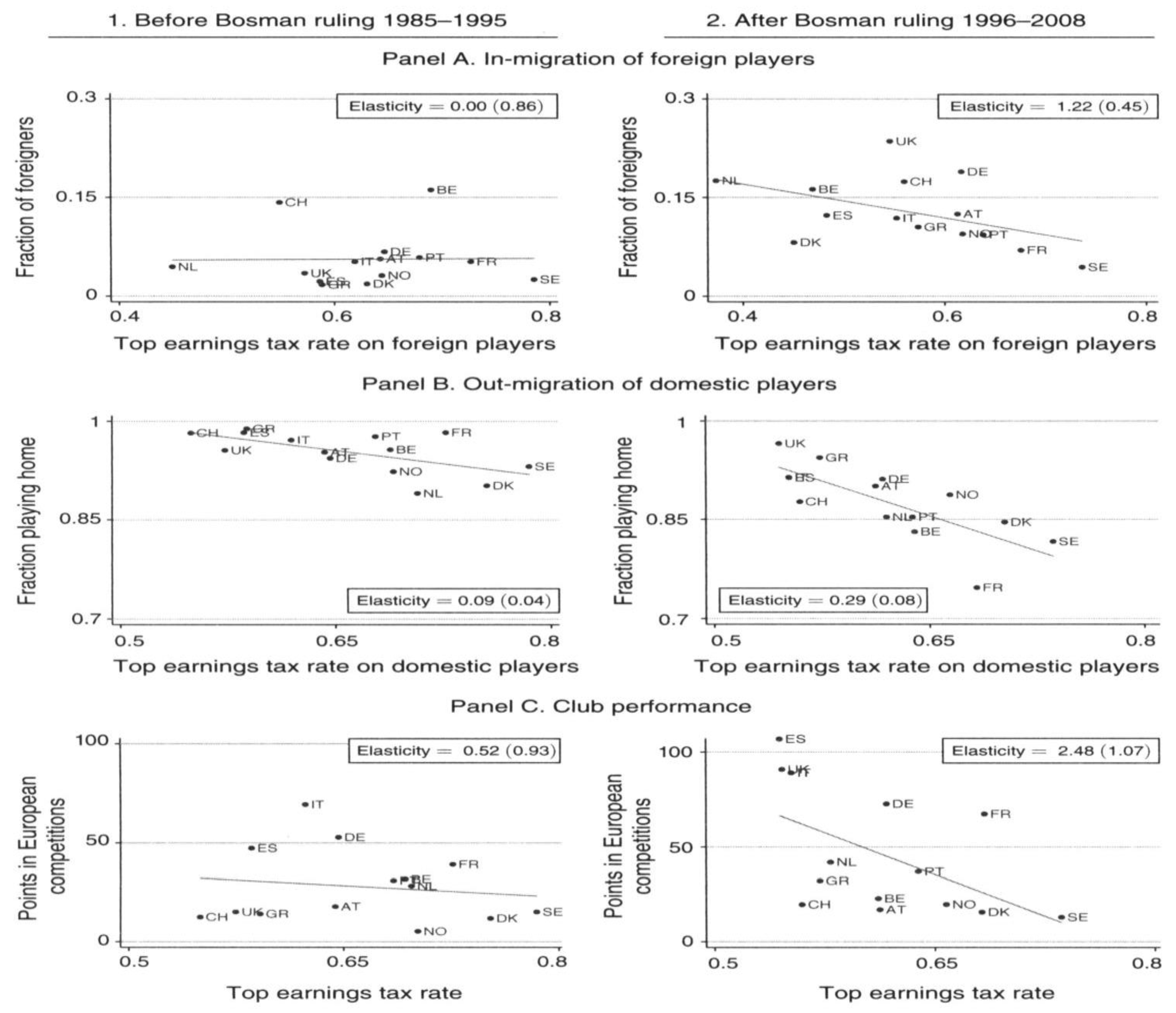
In the pre-Bosman period, the fraction of foreigners is generally very low and there is no correlation between the fraction of foreigners and tax rates. After the Bosman ruling, the fraction of foreigners is much higher in every country (between 5 percent and 25 percent), and there is a significant negative correlation with top earnings tax rate. The implied elasticity of the fraction of foreigners with respect to the net-of-tax rate is zero pre-Bosman era, but very large at 1 .22 (0.45) in the post-Bosman era. Panel B of
Figure 1 plots the average fraction of players of a given nationality playing in their home league against the average top earnings tax rate on domestic residents. In the pre-Bosman era, the fraction of players playing at home is very in all countries (between 90 percent and 100 percent across the entire sample). After the Bosman ruling, the fraction playing at home drops in almost all countries, and negative correlation with tax rates becomes much stronger. The implied elasticity of the fraction playing at home respect to the net-of-tax rate was modest pre-Bosman at 0.09 (0.04) and much post-Bosman at 0.29.
The elasticities are always for foreign players and are obtained from a 2SLS regression of (see Notes to
Table 1 at page 1906 of the original paper)
instrumented with
I(c = T) × I(t > t
0), where
c is country (the treatment country is T i.e.
a synthetic control) and
P is the number of foreign players,
τ is the Top Marginal Tax Rate,
t is the year, and
t0 is the year of the reform.
Possible limitations are the following
In the graphical analysis, the elasticities of the Average Tax Rate are not presented for the pre-Bosman period and the Danish case studies because of lack of individual earnings data before 1996. Similarly, the average tax rate elasticity for Spain is based on the 1996-2003 versus 2004-2008 comparison. It is therefore difficult to conduct a complete comparison study (not even graphical).
The sample used is limited to a very special category of privileged migrants (the well-paid football players whose behaviour is affected by several treatment-related confounding factors). Out of sample projections seems problematic.
Bosman ruling could have had differential impacts on low-tax and high-tax countries for nontax reasons. Tax rates may correlate with country size and thus league quality. Better leagues may have benefited more from Bosman ruling.
Football players contracts are generally signed in advance with respect of the year of the actual transfer and then anticipation effects of the Borman ruling might be present.
Other factors could have changed from the pre-Bosman to the post-Bosman era that impacted low-tax and high-tax countries differentially.
10.3. Toxic Emission and the Environment (Zhou, Zhang, Song, and Wang, 2019; Dong, Li, Qin, Zhang, Chen, Zhao, and Wang, 2022)
Emission trading (buying and selling permissions to pollute the environment by releasing CO2 particles…) is supposed to be a market-driven mechanism able to reduce carbon intensity production processes. It has been widely used in western countries, and it has produced debatable results in terms of reduction of TONs of carbon emissions and emission price determination. In 2013 the Chinese government established pilot carbon emission trading programs in seven provinces. The papers discussed in this section conduct an empirical analysis, using a decomposition and DiD approach of the effects of the 2013 environmental policy. The main conclusions are as follows: (1) Overall, China’s emission trading pilots have driven a significant decline in the carbon intensity, resulting in an average annual decline of approximately 0.026 tons/10,000 yuan in the pilot provinces. (2) In the sample period, emission trading pilots had a sustained and stable effect on carbon intensity with no time lag. (3) Emission trading pilots reduce the carbon intensity by adjusting the industrial structure. In contrast, energy structure and energy intensity channels have not yet been realized.
Zhou, Zhang, Song, and Wang, (2019, 516) use a Propensity Score Matching (PSM) approach before the implementation of DiD to enhance the selection of the appropriate control group from the untreated provinces. According to the authors, this helped solve possible endogenous problems and ensure that the DiD estimation results were unbiased.
After establishing the control group, the DiD approach was used by Zhou, Zhang, Song, and Wang, (2019, 517) to evaluate the overall effect of emission trading pilots on carbon intensity:
Where i denotes provinces and t denotes years.
Dif_CI denotes first-order differences in the carbon intensity (dependent variable); α is the coefficient of the independent variable with α
3 corresponding to the ATET; γ
i and γ
t represent province-fixed and time-fixed effects, respectively; and
e is the random error.
Y correspond to years with the new regulation and
R the regulated (pilot) provinces/units.
In the following table (
Table 3 in the original paper), column (1) reports the results of the fixed effect estimation based on matched data. The coefficient of the variable Y×R was significantly negative. This indicates that implementing the emission trading pilots resulted in an average annual decrease in the carbon intensity of 0.026 tons/10,000 yuan. In addition, column (2) reports the results based on panel data; the results are consistent with column (1), indicating robust estimation results. Columns (3) and (4) show the DID estimation results using non-matched data. The pilots have no significant effect on the downward trend in carbon intensity. This may be because the control group, before matching, included provinces in the western regions. The western regions have experienced a rapid drop in carbon intensity, weakening the significance of pilot effects on reducing carbon intensity. Using the PSM approach to remove the unsuitable provinces from the control group can ensure the DID approach generates unbiased estimation results. They are reported below.
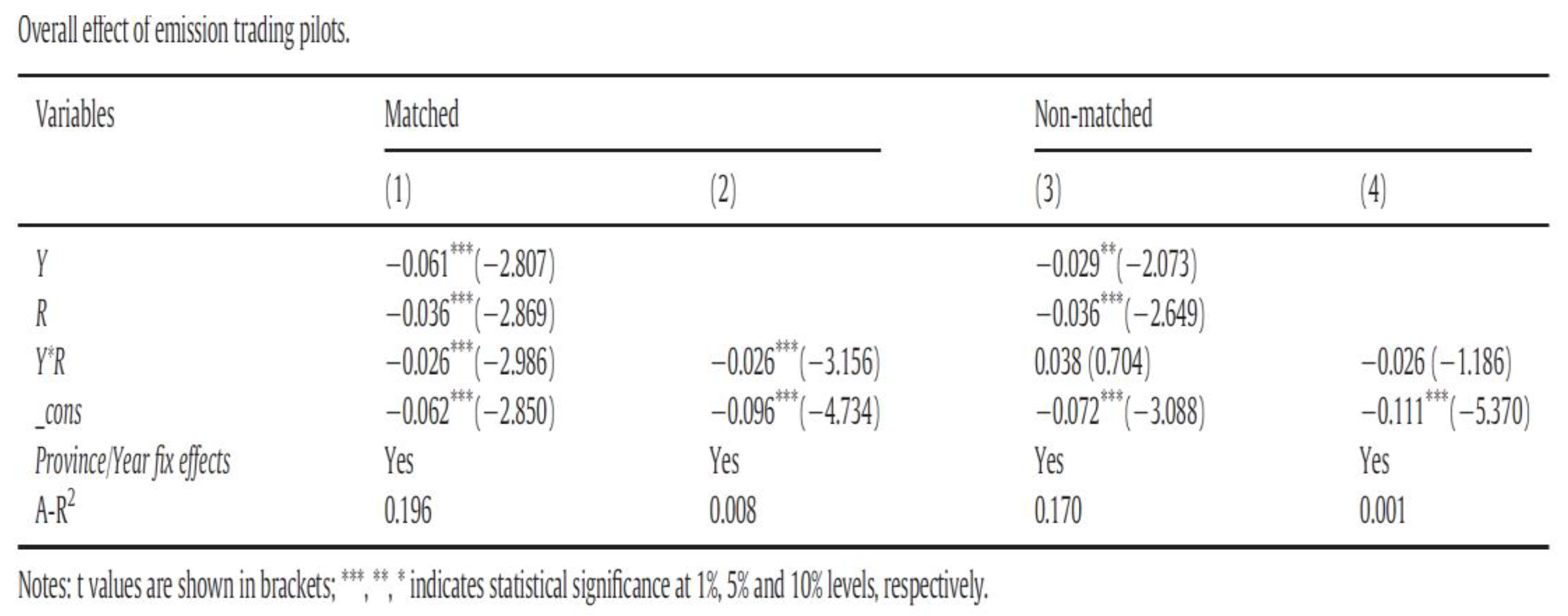
Authors interpret their DiD results as an indication that the adoption of the emission trading reform has effectively reduces China’s carbon intensity.
Similar results are provided by Dong, Li, Qin, Zhang, Chen, Zhao, and Wang (2022, 12) who also estimate the effects of the infrastructure transformation and Greenhouse gas emission performance improvement. Their DiD results show that information infrastructure exerts significant emission reduction compression in cities with large size, advanced digital economy, and leading economic status, while its impact on Greenhouse gas emission performance drops in other cities.
10.4. Regulation, Privatization, Management (Galiani, Gertler, and Schargrodsky, 2005; Gertler et al. 2016)
Galiani, Gertler, and Schargrodsky (2005) and Gertler et al. (2016) study the impact of privatizing water services on child mortality in Argentina. Using a decade of mortality data and comparing areas with privatized (treatment) and non-privatized water companies (control), they observe similar pre-reform (pre-1995) trends that support the parallel trends assumption of their DiD work (plot a of the figure reproduced below).
The authors go on to find a statistically significant reduction in child mortality in areas with privatized water services.
Panel (b) of the figure provides another example, with data on a health variable before (and after) the 2006 Massachusetts reform, as illustrated by Courtemanche and Zapata (2014). A more formal approach to provide support for the parallel trends assumption was followed by conducting a placebo regression, which apply the DiD method to the pre-reform data itself. There should then be no significant “treatment effect”. When running such placebo regressions, one option is to exclude all post-treatment observations and analyse the pre-reform periods only (if there is enough data available).
A line of investigation similar to the one quoted above is provided by Schnabl (2012). He studies the effects of the 1998 Russian financial crisis on bank lending, uses two years of pre-crisis data for a placebo test whereas an alternative is to use all data and add to the regression specification interaction terms between each pre-treatment period and the treatment group indicator(s). The latter method is used by Courtemanche and Zapata (2014), studying the above Massachusetts health reform. A further robustness test of the DiD method is to add specific time trend-terms for the treatment and control groups, respectively, in equations like our equation (1) of section 1.1, and then check that the difference in trends is not significant (see, Wing et al., 2018, p. 459). A general review of the above papers is Fredriksson and Magalhães de Oliveira (2019).
Author Contributions
Conceptualization, B. B. and P.M.; methodology, B. B. and P. M.; software, P.M.; investigation, B.B.; resources, B.B. and P.M.; writing—original draft preparation, B.B. and P.M.; writing—review and editing, B.B.; supervision, P.M. Both authors have read and agreed to the published version of the manuscript.
Funding
This research work was partially funded by the University of Milan-Bicocca (FAR research funds).
Data Availability Statement
All the data used in the examples are included in the Appendix of the paper.
Acknowledgments
This research work was partially supported by the University of Milan-Bicocca.
Conflicts of Interest
The authors declare that there are no conflicts of interest regarding the publication of this paper. The research was conducted independently, and no financial, personal, or professional relationships could be construed as influencing the findings or interpretations presented in this study. Additionally, there are no competing interests related to the funding, data collection, or analysis that could affect the integrity of the research.
Appendix A. An Example with an Easy Visualization of the Data Set
Assume there are 3 randomly selected groups of consumers A, B, and C whose consumption is recorded from 2000 until 2006. For simplicity, each group is composed by 5 people. At the beginning of 2003 a treatment (a commodity tax reduction) is introduced by the local governments where A and B live, and it is maintained till 2006 included. Therefore, we are dealing with 2 period model: the first period/phase (3 years) without any treatment and the second period/phase (4 years) with the treatment affecting some unites. There are barriers that do not permit consumers C to move to locality with lower taxes.
To conduct a simple DiD study, data should be arranged as shown in
Table 2 reproduced in the Appendix. The first column shows Years; the second shows the response variable (the first pedis refers to the individual; the second to her/his group; the third to the year); the rest of the columns show the two dummies and their product.
Table 2 is a basic example of data stuck in panel data form. Groups A and B received the treatment (tax reduction) all in the same year and group C was never treated. The other assumption implicit in
Table 1 is that, once introduced, the treatment was permanent. Hence, in the example we have purposely avoided the complication represented by the differential treatment timing, where different units or groups affected by the treatment start or end their treatment at different times. A special case is when the treatment groups remain permanently affected by treatments that start in different periods. The case is called staggered treatment (different time of a permanent treatment introduction for different groups/units) and will be discussed later in section 7. The case of
Table 2 (same treatment periods for each treated units) is called treatment effect homogeneity.
References
- Angrist J. D. and J.-S. Pischke (2009), Mostly Harmless Econometrics: An Empiricist’s Companion. Princeton University Press.
- Angrist J. D. and J.-S. Pischke (2010), The Credibility Revolution in Empirical Economics: How Better Research Design is Taking the Con out of Econometrics. Journal of Economic Perspectives, 24, 2, p. 3–30.
- Angrist, J. D., G. W. Imbens, & D. B Rubin, (1996). Identification of Causal Effects Using Instrumental Variables. Journal of the American Statistical Association, 91(434), 444-455. [CrossRef]
- Ashenfelter O. & D. Card (1985) Using the Longitudinal Structure of Earnings to Estimate the Effect of Training Programs The Review of Economics and Statistics, 67, 4, pp. 648-660.
- Bertrand, M., E. Duflo, & S. Mullainathan (2004), How much should we trust difference-in-differences estimates? Quarterly Journal of Economics 119: 249–275. [CrossRef]
- Bester, C. A., T. G. Conley, and C. B. Hansen (2011), Inference with dependent data using cluster covariance estimators. Journal of Econometrics 165: 137–151. [CrossRef]
- Bilinski A. and L. Hatfield (2020), Nothing to See Here? Non-Inferiority Approaches to Parallel Trends and Other Model Assumptions, JSM 2020 Virtual Conference, august, https://ww2.amstat.org/meetings/jsm/2020/onlineprogram/AbstractDetails.cfm?abstractid=312323.
- Borusyak, Kirill, Jaravel, Xavier, 2018. Revisiting Event Study Designs. SSRN Scholarly Paper ID 2826228, Social Science Research Network, Rochester, NY.
- Callaway B. (2022), Difference-in-Differences for Policy Evaluation, in K. F. Zimmermann (ed.), Handbook of Labor, Human Resources and Population, pp. 1–61 . [CrossRef]
- Callaway B. and P. Sant’Anna (2021), Difference-in-differences with multiple time periods. Journal of Econometrics 225, pp. 200–230. [CrossRef]
- Cameron A. C. and P. K. Trivedi (2005) Microeconometrics: Methods and Applications, Cambridge University Press.
- Card D. and A. Krueger (1994), Minimum Wages and Employment: A Case Study of the Fast-Food Industry in New Jersey and Pennsylvania, American Economic Review, 84, issue 4, p. 772–93.
- Cerqua, A., Letta, M., and Menchetti, F. (2022). Losing control (group)? The Machine Learning Control Method for counterfactual forecasting.
- Cerqua, A., Letta, M., and Menchetti, F. (2023). The Machine Learning Control Method for Counterfactual Forecasting.
- Cerulli G. (2015), Econometric evaluation of socio-economic programs. Theory and applications. Springer-Verlag GmbH.
- Chesnaye N., Stel S., Tripepi G., Dekker F. W., Fu E. L., Zoccali G., and Jager K. J. (2022), An introduction to inverse probability of treatment weighting in observational research, Clinical Kidney Journal, 15, 1, pp. 14–20 doi: 10.1093/ckj/sfab158.
- Cole, S. R., and Frangakis, C. E. (2009). The Consistency Statement in Causal Inference: A Definition or an Assumption? Epidemiology, 20(1), 3-5. [CrossRef]
- Cox, D. R. (1958). Planning of experiments, Wiley Series in Probability and Statistics - Applied Probability and Statistics Section.
- de Chaisemartin C. and X. D’Haultfoeuille (2020), Two-Way Fixed Effects Estimators with Heterogeneous Treatment Effects, American Economic Review vol. 110, 9, pp. 2964–96.
- de Chaisemartin C. and X. D’Haultfoeuille (2023), Two-way fixed effects estimators with heterogeneous treatment effects: a survey, Econometrics Journal, 26, pp. C1–C30 . [CrossRef]
- Delgado, M. S., and Florax, R. J. G. M. (2015). Difference-in-differences techniques for spatial data: Local autocorrelation and spatial interaction. Economics Letters, 137, 123-126. [CrossRef]
- Elhorst, J. P. (2010). Applied Spatial Econometrics: Raising the Bar. Spatial Economic Analysis, 5(1), 9-28. [CrossRef]
- Fisher, R. A. (1935), Design of Experiments, Oliver and Boyd.
- Freyaldenhoven, S., C. Hansen, and Shapiro, J. (2019), Pre-event Trends in the Panel Event-study Design”, American Economic Review, 109, pp. 3307–3338.
- Goodman-Bacon A. (2021), Difference-in-differences with variation in treatment timing, Journal of Econometrics, 225, 2, pp. 254-277.
- Huber, M., and Steinmayr, A. (2021). A Framework for Separating Individual-Level Treatment Effects From Spillover Effects. Journal of Business and Economic Statistics, 39(2), 422-436. [CrossRef]
- Imbens G. W. and D. B. Rubin (2015), Causal Inference for Statistics, Social, and Biomedical Sciences: An Introduction, Cambridge University Press.
- Kahn-Lang, A. and Lang, K. (2020), The Promise and Pitfalls of Differences-in-Differences: Reflections on 16 and Pregnant and Other Applications, Journal of Business and Economic Statistics, 38, pp. 613–620.
- Laffers, L., and Mellace, G. (2020). Identification of the average treatment effect when SUTVA is violated. Discussion Papers on Business and Economics, University of Southern Denmark, 3.
- Myint L. (2024), Controlling time-varying confounding in difference-in-differences studies using the time-varying treatments framework. Health Services and Outcomes Research Methodology, 24, pp.95–111 . [CrossRef]
- Ogburn, E. L., Shpitser, I., and Lee, Y. (2020). Causal Inference, Social Networks and Chain Graphs. Journal of the Royal Statistical Society Series A: Statistics in Society, 183(4), 1659-1676. [CrossRef]
- Ogburn, E. L., Sofrygin, O., Díaz, I., and van der Laan, M. J. (2024). Causal Inference for Social Network Data. Journal of the American Statistical Association, 119(545), 597-611. [CrossRef]
- Qiu, F., and Tong, Q. (2021). A spatial difference-in-differences approach to evaluate the impact of light rail transit on property values. Economic Modelling, 99, 105496. [CrossRef]
- Rambachan A. and J. Roth (2023), A More Credible Approach to Parallel Trends, Review of Economic Studies 90, pp. 2555–2591.
- Rosenbaum P. R. (1984), The Consequences of Adjustment for a Concomitant Variable That Has Been Affected by the Treatment. Journal of the Royal Statistical Society. Series A (General), 147, 5, pp. 656-666.
- Roth J. (2022), Pretest with Caution: Event-Study Estimates after Testing for Parallel Trends, American Economic Review: Insights, 4, 3, pp. 305–22.
- Roth J., P. Sant’Anna, A. Bilinski, and J. Poe (2023), What’s trending in difference-in-differences? A synthesis of the recent econometrics literature, Journal of Econometrics 235, pp. 2218–2244.
- Rubin, D. B. (1978), Bayesian Inference for Causal Effects: The Role of Randomization, Annals of Statistics, Vol. 6: pp. 34–58.
- Rubin, D. B. (1980), Randomization Analysis of Experimental Data: The Fisher Randomization Test Comment, Journal of the American Statistical Association, Vol. 75, pp. 591-593. Rubin, D. B. (1990), Formal Modes of Statistical Inference for Causal Effects, Journal of Statistical Planning and Inference, Vol. 25: pp. 279–292.
- Rubin, D. B. (1980). Randomization Analysis of Experimental Data: The Fisher Randomization Test Comment. Journal of the American Statistical Association, 75(371), 591-593. [CrossRef]
- Rubin, D. B. (1990). [On the Application of Probability Theory to Agricultural Experiments. Essay on Principles. Section 9.] Comment: Neyman (1923) and Causal Inference in Experiments and observational Studies. Statistical Science, 5(4), 472-480, 479. [CrossRef]
- Schwartz, S., Gatto, N. M., and Campbell, U. B. (2012). Extending the sufficient component cause model to describe the Stable Unit Treatment Value Assumption (SUTVA). Epidemiologic Perspectives and Innovations, 9(1), 3. [CrossRef]
- Sobel, M. E. (2006). What Do Randomized Studies of Housing Mobility Demonstrate? Journal of the American Statistical Association, 101(476), 1398-1407. [CrossRef]
- Sun, S., and Delgado, M. S. (2024). Local spatial difference-in-differences models: treatment correlations, response interactions, and expanded local models. Empirical Economics. [CrossRef]
- VanderWeele, T. J. (2009). Concerning the Consistency Assumption in Causal Inference. Epidemiology, 20(6), 880-883. [CrossRef]
- VanderWeele, T. J. (2010). Direct and Indirect Effects for Neighborhood-Based Clustered and Longitudinal Data. Sociological Methods and Research, 38(4), 515-544. [CrossRef]
- VanderWeele, T. J., Tchetgen, E. J. T., and Halloran, M. E. (2015). Interference and sensitivity analysis. Statistical science: a review journal of the Institute of Mathematical Statistics, 29(4), 687.
- Wang, Y. (2021). Causal Inference with Panel Data under Temporal and Spatial Interference. arXiv preprint arXiv:2106.15074.
- Wang, Y., Samii, C., Chang, H., and Aronow, P. (2020). Design-based inference for spatial experiments under unknown interference. arXiv preprint arXiv:2010.13599.
- Wooldridge J. M. (2010), Econometric Analysis of Cross Section and Panel Data, Second Edition, The MIT Press.
- Wooldridge, J. M. (2021), Two-Way Fixed Effects, the Two-Way Mundlak Regression, and Difference-in-Differences Estimators, Available at SSRN: https://ssrn.com/abstract=3906345. [CrossRef]
- Wooldridge, J. M. (2023), Simple approaches to nonlinear difference-in-differences with panel data. Econometrics Journal, 26, pp. C31–C66 . [CrossRef]
- Xu, Y. (2024). Causal Inference with Time-Series Cross-Sectional Data: A Reflection. In J. M. Box-Steffensmeier, D. P. Christenson, and V. Sinclair-Chapman (Eds.), Oxford Handbook of Engaged Methodological Pluralism in Political Science (pp. 0). Oxford University Press. [CrossRef]
- Zeldow B. and L.A. Hatfield (2021), Confounding and regression adjustment in difference-in-differences studies, Health Services Research 56, pp. 932–941 . [CrossRef]
References for Section 10 (Applications) and Further Readings
Abadie A., A. Diamond, A., & J. Hainmueller (2015). Comparative Politics and the Synthetic Control Method. American Journal of Political Science. 59 (2): pp. 495–510
https://doi.org/10.1111/ajps.12116
Bosco B.P., C.F. Bosco, & P. Maranzano (2025). Labour responsiveness to income tax changes: empirical evidence from a DID analysis of an income tax treatment in Italy. Empirical Economics
https://doi.org/10.1007/s00181-025-02748-7
Courtemanche, C. J., and D. Zapata (2014). Does universal coverage improve health? The Massachusetts experience. Journal of Policy Analysis and Management, 33, pp. 36–69.
Dong F., Y. Li, C. Qin, X. Zhang, Y. Chen, X. Zhao, and C. Wang (2022), Information infrastructure and greenhouse gas emission performance in urban China: A difference-in-differences analysis, Journal of Environmental Management 316, 115252
https://doi.org/10.1016/j.jenvman.2022.115252
Feldstein M. (1995), The Effect of Marginal Tax Rates on Taxable Income: A Panel Study of the 1986 Tax Reform Act, Journal of Political Economy, 103, pp. 551–572.
Feldstein M. (1999), Tax Avoidance And The Deadweight Loss Of The Income Tax, The Review of Economics and Statistics, 81(4): pp. 674-680
Fredriksson A., and G. Magalhães de Oliveira (2019), Impact evaluation using Difference-in-Differences, RAUSP Management Journal, 54, 4, pp. 519-532
Galiani, Gertler, and Schargrodsky (2005), Water for life: The impact of the privatization of water services on child mortality. Journal of Political Economy, 113, pp. 83–120.
Gertler, P. J., Martinez, S., Premand, P., Rawlings, L. B., and Vermeersch, C. M. (2016). Impact evaluation in practice, Washington, DC: The World Bank.
Goolsbee A. (2000), What Happens When You Tax the Rich? Evidence from Executive Compensation, Journal of Political Economy, 108, pp. 352–378.
Jakobsen K., K. Jakobsen, H. Kleven, and G. Zucman (2020), Wealth Taxation and Wealth Accumulation: Theory and Evidence from Denmark, The Quarterly Journal of Economics, 135(1), pp. 329–388.
Johannesen N. and G. Zucman (2014), The End of Bank Secrecy? An Evaluation of the G20 Tax Haven Crackdown, American Economic Journal: Economic Policy, 6(1), pp. 65–91.
Kleven H., J. M. Knudsen, C. Kreiner, S. Pedersen, and E. Saez (2011), Unwilling or Unable to Cheat? Evidence from a Tax Audit Experiment in Denmark, Econometrica, 79(3), pp. 651–692.
Kleven k. J., C. Landais, E. Saez (2013), Taxation and International Migration of Superstars: Evidence from the European Football Market, American Economic Review, 103(5), pp. 1892–1924.
Moretti E. and D. J. Wilson (2017), The Effect of State Taxes on the Geographical Location of Top Earners: Evidence from Star Scientists, American Economic Review 107, 7, pp. 1858-1903
Naritomi J. (2019), Consumers as Tax Auditors, American Economic Review, 109(9), pp. 3031–3072.
Schnabl, P. (2012). The international transmission of bank liquidity shocks: Evidence from an emerging market. The Journal of Finance, 67, pp. 897–932
Tørsløv T., L. Wierand, and G. Zucman (2023), Externalities in International Tax Enforcement, American Economic Journal: Economic Policy, vol. 15, 2, pp. 497–525.
Zhou B., C. Zhang, H. Song, and Q. Wang (2019), How does emission trading reduce China’s carbon intensity? An exploration using a decomposition and difference-indifferences approach, Science of the Total Environment 676, pp. 514–523.
https://doi.org/10.1016/j.scitotenv.2019.04.303
| 1 |
Callaway (2022) discusses an ampler set of estimation strategies. According to Callaway (2022, 4) all of them explicitly make, in a first step, the same good comparisons that show up in the TWFE regression (i.e., the comparisons that use units that become treated relative to units that are not-yet-treated) while explicitly avoiding the “bad comparisons” that show up in the TWFE regression (i.e., the comparisons that use already-treated units as the comparison group). Then, in a second step, they combine these underlying treatment effect parameters into target parameters of interest such as an overall average treatment effect on the treated. See Section Alternative Approaches in Callaway (2022, 20). |
| 2 |
A number of different ICC statistics have been proposed, not all of which estimate the same population parameter. There has been considerable debate about which ICC statistics are appropriate for a given use, since they may produce markedly different results for the same data |
| 3 |
A list of bias correction procedures is provided by Angrist and Pischke (2009, p. 320-2). |
| 4 |
In a later paper (Feldstein, 1999) he also argues that traditional analyses of the income tax greatly underestimate deadweight losses by ignoring its effect on forms of compensation and patterns of consumption. He calculated the full deadweight loss using the compensated elasticity of taxable income to changes in tax rates because leisure, excludable income, and deductible consumption are assumed (by Feldstein) to be a Hicksian composite good. According to his estimations a deadweight loss of as much as 30% of revenue or more than ten times Harberger’s classic 1964 estimate. The relative deadweight loss caused by increasing existing tax rates is substantially greater and, according to Feldstein’s results, may exceed $2 per $1 of revenue. Some enormous measure, one should say! |
| 5 |
The treatment incorporated in the Feldstein’s analysis was the 1986 US tax reform that lowered marginal tax rates, and simultaneously broadened tax bases. The two elements were designed to net out. Approximately no revenue and distributional effects absent behavioural responses means that approximately there are no income effects. Important as the aim is to estimate the compensated elasticity of taxable income. |
| 6 |
This Review does not discuss synthetic controls. One should see Abadie et al (2015). A synthetic control can be constructed as a weighted average of several units combined to recreate the trajectory that the response variable of a treated unit would have followed in the absence of the treatment. |
| 7 |
This is in contrast with the view that the appropriate tax rate for decisions on the intensive margin is the marginal tax rate (MTR = tax rate on the last euro earned). In the paper ATR is not exact but approximated (for a subsample of football players). Since these taxpayers earn very high salaries, authors approximate the ATR by the top marginal tax rate (MTR). An alternative, and possible more reliable procedure is followed by Moretti and Wilson (2017). By focusing on the locational outcomes of star scientists, defined as scientists with patent counts in the top 5 percent of the distribution, their paper quantifies how sensitive is migration by these stars to changes in personal and business tax differentials across states in the USA. The study uncovers large, stable, and precisely estimated effects of personal and corporate taxes on star scientists’ migration patterns. The long-run elasticity of mobility relative to taxes is 1.8 for personal income taxes, 1.9 for state corporate income tax, and -1.7 for the investment tax credit. |
|
Disclaimer/Publisher’s Note: The statements, opinions and data contained in all publications are solely those of the individual author(s) and contributor(s) and not of MDPI and/or the editor(s). MDPI and/or the editor(s) disclaim responsibility for any injury to people or property resulting from any ideas, methods, instructions or products referred to in the content. |
© 2025 by the authors. Licensee MDPI, Basel, Switzerland. This article is an open access article distributed under the terms and conditions of the Creative Commons Attribution (CC BY) license (http://creativecommons.org/licenses/by/4.0/).