Submitted:
12 August 2025
Posted:
15 August 2025
You are already at the latest version
Abstract
Since Roth’s work on the generalized Sylvester equation AX −YB = C (GSE) in 1952, related research has consistently attracted significant attention. Building on this, this review systematically summarizes relevant research on GSE from five perspectives: research methods, constrained solutions, various generalizations, iterative algorithms, and applications. Furthermore, we provide comments on current research, put forward several intriguing questions, and offer prospects for future research trends. We hope this work can fill the gap in the review literature on GSE and offer some inspiration for subsequent studies in the field.
Keywords:
generalized sylvester equation
; moore-penrose inverse
; matrix decompositions
; semi-tensor product
; constrained solutions
; operator equations
; tensor equations
; polynomial matrix equations
; iterative algorithms
; hand-eye calibration
; encryption and decryption schemes
1. Introduction
This review commences with the famous Sylvester equation
with unknown X, named after the British mathematician James Joseph Sylvester (1814–1897) [251]. For a detailed discussion of this equation, refer to the review article [14] by Rajendra Bhatia, a Fellow of the Indian National Science Academy. The core of our review revolves around the generalized Sylvester equation (abbreviated as GSE):
with unknown X and Y.
In 1952, Roth established the necessary and sufficient conditions for the solvability of GSE over a field by means of block matrix equivalence. Since then, a large number of papers on GSE have been published in rapid succession. The solvability conditions and explicit expressions of the general solution for GSE have been investigated from diverse perspectives: linear transformations, generalized inverses, matrix decompositions, real (complex) representations, determinant representations, and semi-tensor products, etc. Extensive studies have been conducted on various constrained solutions (e.g., ★-congruent, symmetric, self-adjoint, positive (semi)definite, per(skew)symmetric, bi(skew)symmetric, Re-(non)negative definite, Re-(non)positive definite, -Hermitian, -skew-Hermitian, -Hermitian, and equality-constrained solutions) of GSE, as well as its various best approximate solutions when the solvability conditions are not satisfied. Furthermore, the generalizations of GSE in different algebraic structures (e.g., unit regular rings, principal ideal domains, division rings, module-finite rings, commutative rings, Artinian rings, noncommutative rings, dual numbers, dual quaternions), operator equations, tensor equations, polynomial matrix equations, Sylvester-polynomial-conjugate matrix equations, and formal aspects have also shown remarkable vitality. Iterative algorithms for solving various solutions to GSE and its extended forms have also attracted considerable attention, with continuous updates and optimizations. Finally, the relevant results of GSE have demonstrated extraordinary significance in both theoretical applications (e.g., solvability of matrix equations, dual number matrix factorizations, and microlocal triangularization of pseudo-differential systems) and practical applications (e.g., hand-eye calibration problems, and encryption and decryption of color images).
Qing-Wen Wang, the first author of this paper, has been engaged in researching and teaching on the theory of matrix equations since the early 1990s, and has published over 100 related articles. Numerous scholars both domestically and internationally have suggested that we systematically present the theory of solving linear matrix equations. To date, our team has published three review articles, focusing respectively on solving the equations [284], and [278], as well as and [279].
As mentioned earlier, in the development history of research on GSE, its conclusions are interrelated, mutually inspiring, mutually promotive, and progressively advanced, forming a complex, intertwined, and extensive network. By reviewing numerous literature, analyzing and comparing, summarizing, questioning, and prospecting, we strive to identify the commonalities, main threads, and approaches in these studies, aiming to provide insights and inspiration for subsequent research on GSE. Thus, this work is of significant value. In this paper, we intend to focus on GSE as the core theme, and unfold its solution methods, solution categories, generalizations, iterative algorithms, as well as theoretical and practical applications in a step-by-step manner, so as to provide a comprehensive overview.
The remainder of this paper consists of 8 sections. Section 2 presents some necessary notations and notes. In Section 3, we introduce Roth’s work on GSE published in [228], which serves as the starting point for this paper. In Section 4, we summarize seven methods for studying GSE, demonstrating diverse perspectives and research schemes. Various solutions to GSE are discussed in detail in Section 5. We devote Section 6 to introducing the generalizations of GSE in certain algebraic aspects. In Section 7, we enumerate several classic iterative algorithms for solving various solutions to GSE and its generalized forms. The theoretical and practical applications of GSE are presented in Section 8. Conclusions are stated in Section 9.
2. Preliminary
This section recalls some notations and definitions used throughout the paper. Additionally, other necessary terminology for subsequent (sub)sections will be introduced within each. A few symbols, due to their bulk, will be referenced via specific indices in original sources, rather than being reproduced. This not only does not hinder readers’ understanding but also makes the paper more concise and readable.
Let be a ring; let be the polynomial ring over with the variable ; let be the set of all matrices over ; let be the set of all polynomial matrices over with the variable . Specially, . Let be the degree of ; let be the rank of ; let be the transpose of . The symbol denotes the determinant of for a field . The component-wise representation of can be denoted in the following three forms:
The Kronecker product of and is defined by
The matrices and are equivalent if there exist two nonsingular matrices and such that . Moreover, and are equivalent if there exist two invertible polynomial matrices and such that .
For a subspace , let be the orthogonal projector onto ; and let and be the orthogonal complement and dimension of , respectively. In addition, denote for . For two vector spaces V and W over a field F, let be a linear transformation from V to W; then and represent the kernel space and the image of , respectively.
Let , , , and be the sets of all positive integers, natural numbers, real numbers, and complex numbers, respectively. The symbol stands for the sign of , and ∅ represents the empty set. Let the set of all (real) quaternions be
which is a four-dimensional noncommutative division algebra over [227]. Let the conjugate of a quaternion be
Let . The conjugate of A is , and the conjugate transpose of A is . Let
where . If () for , then A is called -Hermitian (-anti-Hermitian) [127]. An -anti-Hermitian matrix is also called an -skew-Hermitian matrix. Moreover, and for .
Denote
where is the Moore-Penrose inverse [215] of a matrix A. The symbols , , , and denote the inverse, rank, range, and null space of a matrix A, respectively. In addition, , , and are the conjugate, conjugate transpose, and Frobenius norm of , respectively. Let I and 0 be the identity matrix and the null matrix, respectively, with appropriate orders. Specifically, denotes the identity matrix. For a symmetric matrix , and denote the positive definite matrix and the positive semidefinite matrix, respectively. In addition, denote if for matrices A and B. The matrix
denotes a new matrix formed by arranging matrix blocks (with the same number of rows) column-wise. The symbol denotes a (block) diagonal matrix with diagonal entries .
For a ring and , a is regular (or inner-invertible) if there exists such that ; a is -invertible (or reflexive) if there exists such that and . The characteristic of a field is denoted as .
An equation or a system of equations is said to be solvable (consistent) if it has at least one solution. The symbols “⇒" and “⇔" denote “imply" and “if and only if", respectively.
At the end of this section, we present three specific notes regarding this review.
- (1)
- Though some research does not focus directly on GSE itself, its traces are easily detectable. Thus, we regard such content as an integral part of GSE-related research.
- (2)
- We selected core literature relevant to this review. Results closely related to the theme are rigorously presented as theorems, while less relevant conclusions are briefly summarized narratively. Furthermore, the proofs of these theorems are omitted here.
- (3)
- The remarks in this paper include comments and suggestions on relevant results, encompassing both previous researchers’ views and our reflections, questions, and prospects.
3. Roth’s Equivalence Theorem
First, we specifically present the paper’s core equation:
where , , and are given over a ring .
Let be a field. In 1952, Roth [228] first studied the necessary and sufficient conditions for the solvability to the polynomial matrix form of Eq. (1), i.e.,
where , by using the normal form of polynomial matrices.
Roth [228], Theorem 1 has stated that Theorem 1 still valid for rectangular polynomial matrices of appropriate orders. Thus, the following theorem can be derived immediately.
Theorem 2.
[228], Theorem 1 Let , , and . Then,
if and only if
We call this theorem Roth’s equivalence theorem (abbreviated as RET).
4. Different Methods on GSE
Roth [228] considered Eq. (1) based on the canonical forms of the polynomial matrices. Subsequently, many scholars have provided different proofs of RET from various perspectives. These proofs demonstrate the effectiveness and uniqueness of different mathematical methods in considering Eq. (1). In addition, these methods have also had a profound impact on the subsequent study of different Sylvester-type equations. This is precisely one of the enchantment of mathematics: reaching the same endpoint through different paths, or even completely unrelated ones. Furthermore, mathematicians ceaselessly pursue groundbreaking innovations and perpetually strive to discover the most elegant path.
Remark 2.
4.1. Method by Linear Transformations and Subspace Dimensions
Let be a field. Flanders and Wimmer [80] proved RET for and by means of linear transformations and subspace dimension arguments. This method is more fundamental and elementary than Roth’s method.
Proof of RET. [80]
- Step 1:
-
Define byThen, the condition (4) yields
- Step 2:
-
LetThen,LetFor , defineThen So, .
- Step 3:
- Since with , there also exists such in . Therefore, , i.e., (3) holds. □
Remark 3.
- (1)
- In [80], Flanders and Wimmer mentioned that by making small modifications to the above proof, one can similarly obtain the proof of RET under the condition of rectangular matrices A, B, and C.
- (2)
4.2. Method by Generalized Inverses
Let be a field. In 1955, Penrose [215] concisely defined the Moore-Penrose inverse of any rectangular matrix through four matrix equations.
Definition 1.
Since then, the theory of generalized inverses has flourished (see [9,40,223,265]), and it has been widely used to study the solvability conditions of linear equations and represent the explicit expressions of their general solutions when solvable. Penrose’s study on the matrix equation [215] is the most renowned.
In 1979, Baksalary and Kala [6] naturally utilized inner inverses to establish solvability conditions and representations of the general solution for Eq. (1).
Theorem 3.
in which case,
where W and Z are arbitrary matrices with appropriate orders.
Remark 4.
In views of RET and Theorem 3, Baksalary and Kala [6], Remark 2 noted that
They also pointed out that this result can be directly derived by using [197], Fomula (8.7) in a particular case, i.e.,
Remark 5.
Under the hypotheses of Theorem 3, it is easy to obtain that
Remark 6.
It is easy to show that the solvability of Eq. (1) is equivalent to the existence of X and Y such that
In terms of a geometrical method, Olshevsky gave a cyclic argument over as follows:
(see [209], Proof of Theorem 1.2).
Let . Meyer [201] revealed an interesting result, that is, the solvability of Eq. (1) is equivalent to the existence of the upper block inner inverse of a certain block matrix.
Theorem 4.
[201], Theorems 1 and 2 The block triangular complex matrix
has an upper block triangular inner inverse if and only if
in which case,
is an inner inverse of T for any and .
4.3. Method by Singular Value Decompositions
Let . The singular value decomposition (abbreviated as SVD) [89], as an important tool for the study of matrix theory, also plays a significant role in the research on solutions of matrix equations. Chu [34] utilized the SVD to study the solvability conditions and the representation of the general solution of Eq. (5).
In fact, let the SVDs of A and B given in Eq. (5) be
where , , , and are orthogonal matrices with appropriate orders,
with (), and with (). Then,
where , , and . Partitioning the above equation analogously to the partitioning of and , we obtain
Based on the above discussion, the following theorem can be obtained.
Theorem 5.
Remark 7.
Interestingly, Chu in [34], Theorem 1 utilized the generalized singular value decomposition (abbreviated as GSVD) [212] to study the extended form of Eq. (5) over , i.e.,
where , and C are given real matrices with appropriate orders. Eleven years later, Xu et al. [323] once again discussed the solvability conditions, the general solution, and least-squares solutions of Eq. (12) over by using the canonical correlation decomposition (abbreviated as CCD) introduced in [90].
Remark 8.
Inspired by solving Eq. (5) via SVD, one can utilize equivalent normal forms of A and B to study Eq. (5) over a field, along with an approach similar to Theorem 5. In fact, we only need to regard orthogonal matrices , , , and in (9) as invertible matrices, the transpose and as the inverse and , and and as identity matrices of appropriate orders.
It can be found that using the equivalent normal form of matrices to solve matrix equations is also a very convenient method. This viewpoint has been confirmed multiple times in the subsequent research. Wang et al. used the elementary row and column transformations of matrices to give the equivalent normal form of a matrix triplet
with the same row number over an arbitrary division ring (see [273], Theorem 2.1). Similarly, the equivalent normal form of another matrix triplet
with the same column number can also be obtained (see [273], Theorem 2.2). The two equivalent normal forms are applied to solve the matrix equation
where X, Y, and Z are unknown (see [273], Theorem 3.2).
Interestingly, He et al. utilized [273], Theorem 2.1 to propose a simultaneous decomposition of seven matrices over (see [125], Theorem 2.3), i.e.,
and discussed Eq. (13) once again by this decomposition (see [125], Theorem 3.1). Compared with the method in [273], which directly applies the equivalent normal forms of two matrix triplets to matrix G, the simultaneous decomposition is more concise. In addition, Ref. [114] once again brilliantly demonstrates the important role of simultaneous decomposition in solving matrix equations.
4.4. Method by Simultaneous Decompositions
Let be a field. Remark 8 notes using equivalent canonical forms of the matrices A and B to solve Eq. (1). Can we find an equivalent canonical form that is simultaneously related to the matrix triplet
so as to discuss Eq. (1) more simply? Gustafson [97] gave a positive answer to this problem.
Theorem 6.
[97] Let A, B, and C be given in Eq. (1). Then there exist invertible matrices T, U, V, and W of appropriate orders such that
where
Remark 9.
Theorem 7.
where the and are arbitrary matrices with appropriate orders.
Remark 10.
The quiver theory introduced by Gabriel [84] is an important tool in the representation theory of algebras. Gustafson [97] gave a novel interpretation of the existence of the simultaneous decomposition of (14) from the perspective of the quiver theory. Finally, he gave a necessary and sufficient condition for Eq. (1) to have a solution by using the corresponding representation of arrows (see [97], Section 10). Noted that Refs. [59,115] also make use of the graph theory to discuss linear matrix equations.
Remark 11.
Wang et al. in [276], Theorem 2.1 continued with the idea of simultaneous decomposition and decomposed the following matrices over a division ring :
where A, B, and C are of the same row number, and A and D are of the same column number. So, Theorem 6 is a corollary of [276], Theorem 2.1 (see [276], Corollary 2.2). Also, it should be noted that [273], Theorem 2.1 is indeed a special case of [276], Theorem 2.1 (see [276], Corollary 2.3). In addition, Wang et al. applied the simultaneous decomposition of (17) to solving two types of systems of matrix equations. Interestingly, He et al. [116] further refined the simultaneous decomposition presented by [276].
He et al. [126] further considered the simultaneous decompositions of two more general forms over :
4.5. Method by Real (Complex) Representations
It is well known that a associative algebra with finite dimensions over a field is isomorphic to a subalgebra of the algebra , where n is the dimension of over (see [81]). We now consider the case of complex numbers, i.e., .
Let , where , and is the imaginary unit such that . Define a map
We call a real representation of the complex matrix A[191]. Then, one can check that is an isomorphism of the real algebra onto the real subalgebra
Then,
On the other hand, suppose that a real matrix pair
is a solution pair of the following equation
Then, and are also a solution pair of Eq. (18), where
Based on the above analysis, the problem of a complex matrix equation is transformed into a problem of a real matrix equation by using the real representation of complex matrices. Based on this consideration, Liu [191] proposed the following theorem for solving Eq. (5) over .
Theorem 8.
[191], Lemma 1.3 Let
is consistent over , in which case,
where , and are the general solution of Eq. (19). Furthermore, the explicit forms of X and Y given in (20) are
where ,
and are arbitrary matrices over with appropriate orders.
Remark 12.
Liu [191] further used Theorem 8 to discuss the maximal and minimal ranks of Eq. (5)’s solutions, as seen in SubSection 5.6 of this paper.
Remark 13.
We know that the quaternion algebra (or the quaternion division ring) cannot be a field because it does not satisfy the commutative law. However, when studying matrix equations over , it is widely applied that the method of converting the quaternion matrix equations to the real (or complex) matrix equations by using the real (or complex) representation of quaternions [227]. For example, [337] and [333] studied the special least-squares solutions of a class of quaternion matrix equations by using the real representation and the complex representation of quaternions, respectively. Moreover, the real (or complex) representation of some other quaternions mentioned in Remark 43 have been explored in [190,226,264,332].
On the other hand, because real (or complex) representations have the drawback of a significant increase in computational load, Wei et al. [292] introduced real structure-preserving methods over for LU decomposition, QR decomposition, and SVD, thereby solving quaternion linear systems.
4.6. Method by Determinantal Representations
As is well known, Cramer’s rule for the linear equation for unknown vector x is an effective means of expressing its unique solution. In addition, it can be found in SubSection 4.2 that the theory of generalized inverses is closely related to the study of Eq. (1). Naturally, we can consider whether Cramer’s rule for the solutions of Eq. (1) can be obtained through determinant representations of generalized inverses.
Generalized inverses (especially the MP inverse) over fields (particularly the complex field) have been thoroughly discussed and applied to characterize various solutions of matrix equations (see [9,249,265]). Notably, Kyrchei [169] presented the determinantal representations of the MP inverse and the Drazin inverse [62] from the new perspective of limit representations of generalized inverses in 2008.
When we consider the determinantal representations of generalized inverses in the quaternion algebra, it relies on the theory of determinants of quaternion matrices. However, due to the noncommutativity of quaternions, the determinants of quaternion matrices become much more complicated (see [4,37]). It was not until several decades later, after Kyrchei [168,171] introduced the theory of column-row determinants over , that this problem was effectively solved.
Definition 2
(Column-row determinants over ). [168], Definitions 2.4 and 2.5 Let , and let be the symmetric group on .
- (1)
-
For , the i-th row determinant of A is defined bywhere , and for and .
- (2)
-
For , the j-th column determinant of A is defined bywhere and for and .
Remark 14.
Kyrchei in [168], Theorem 3.1 showed that if is Hermitian, i.e., , then
Thus, [168], Remark 3.1 defines the determinant of a Hermitian matrix A by
We now introduce some necessary notations. Let . Then, , , , and denote the left row space, the right column space, the left null space, and the right null space of A, respectively. Let
where . By , we denote the submatrix of A whose rows are indexed by and whose columns are indexed by . If A is Hermitian, then is the corresponding principal minor of A. For , let
And, for and , let
We denote the j-th column of A by and its i-th row by . And, is the matrix that is obtained from A by replacing its j-th column by the column vector , and is the matrix obtained from A by replacing its i-th row by the row vector . Symbols and denoted the j-th column and the i-th row of , respectively.
Kyrchei [173] obtained the Cramer’s rules for some left, right and two-sided quaternion matrix equations by the theory of the column-row determinants over . Song et al. [246] then utilized results in [173] to further study the Cramer’s rule for the quaternion matrix equation:
where , , , , and are given.
Theorem 9.
Let , L, , and N be of full column rank matrices over such that
Then, the general solution of Eq. (21) is
where
with and are the i-th row and j-th column of
respectively, and and are the i-th column and j-th row of
respectively, for , , , and , where
for arbitrary , , Z, and H with appropriate orders.
Remark 15.
When E and F in Eq. (21) are identity matrices, by Theorem 9 we immediately derived the Cramer’s rule to the matrix equation over :
Note that Theorem 9 uses the auxiliary matrices, i.e., K, L, M, and N, to derive the determinant representation of the general solution of Eq. (22). However, these auxiliary matrices are not always easy to obtain in practical applications. Then, can we obtain the Cramer’s rule for Eq. (22) only through its given coefficient matrices?
In order to answer the above problem, let’s first take a look at another work of Kyrchei [170]. Based on the column-row determinant theory and the limit representation of the MP inverse, he gave the determinant representation of the MP inverse over in [170]. This research has greatly promoted the study of the Cramer’s rules to the various solutions of matrix equations over (see [164,165,166,172,243,244,245]). Denote
Theorem 10.
[170], Theorem 5 Let and . Then,
where and .
A result similar to Theorem 3 was given by Kyrchei in [165].
Theorem 11.
[165], Lemma 5.1 The following are equivalent:
- (1)
- Eq. (22) is solvable;
- (2)
- ;
- (3)
- ;
in which case,
where U, V, and W are arbitrary matrices of appropriate orders over .
It is easy to see that
are the partial solution pair of Eq. (22) by taking U, V, and W as zero matrices in (23). Then, by applying Theorem 10 to (24), Kyrchei [165] presented a new Cramer’s rule for the partial solution of Eq. (22), which only makes use of the coefficient matrices, i.e., A, B, and C.
Theorem 12.
where is the j-th columns of , and
where and are the g-th rows of and , respectively.
Remark 16.
Note that although Kyrchei [165] gave the determinant representation of the particular solution of Eq. (22), the problem proposed in Remark 15 is not solved completely. That is to say, the Cramer’s rule for representing the general solution of Eq. (22) only using the coefficient matrices remains an unsolved problem.
Interestingly, Song [247] considered the determinant representation for the general solution of Eq. (22) with the restricted conditions, i.e.,
where , , , and . Let () denote the right (left) -orthogonal projector onto a right (left) -vector subspace ( ) along .
Theorem 13.
and be such that
- (1)
-
The restricted Eq. (25) is solvable if and only ifin which case,whereand , , , , , and are arbitrary matrices over with appropriate dimensions.
- (2)
-
Let , and be full column rank matrices such thatDenote and . If Eq. (25) is solvable, thenwith is the j-th column ofand is the i-th row ofwhere , , , , and and are arbitrary matrices over with appropriate orders.
4.7. Method by Semi-Tensor Prodcuts
To effectively handle multidimensional arrays and nonlinear problems, Chinese mathematician Daizhan Cheng [30] pioneered a new matrix product in 2001: the semi-tensor product (abbreviated as STP). It exactly coincides with traditional matrix products when the two factor matrices meet the dimension requirements. Due to the excellent properties of STP [26], namely:
- (1)
- It is applied to any two matrices;
- (2)
- It has certain commutative properties;
- (3)
- It inherits all properties of the conventional matrix product;
- (4)
- It enables easy expression of multilinear functions (mappings);
STP has been effectively applied to: Boolean (control) networks, logical dynamic systems, systems biology, graph theory, formation control, finite automata and symbolic dynamics, circuit design and failure detection, coding and cryptography, fuzzy control, engineering, game theory, and so on (see [25,26,27,31,32] and references therein).
Definition 3.
[30] Let be a ring, , and . The left STP of A and B is defined as
where is the least common multiple of n and p.
Remark 17.
Similarly, Cheng [25] defined the right SPT of A and B, i.e.,
However, its mathematical properties are not as good as those of the left STP in certain aspects, accounting for most studies’ focus on the left STP. Therefore, the STP referred to in this paper specifically denotes the left STP.
Remark 18.
As a generalization of the traditional matrix product, and given its extensive application significance, the study of matrix equations under STP has emerged as an inevitable and pivotal research direction. In 2016, Yao et al. [331] were the first to conduct research on the classical complex matrix equation under STP:
where X is unknown. Subsequently, building on the research framework of [331], investigations into diverse matrix equations under STP have flourished (see [137,144,180,266,268,271]).
Regrettably, no studies directly addressing Eq. (5) under STP have been published to date. However, when the dimension of Y is constrained to equal that of , the exploration of Sylvester-transpose matrix equation [137]
with unknown X may provide valuable guidance for this problem.
Since 2020, Liaocheng University’s team led by Professors Ying Li and Jianli Zhao has utilized STP to propose several novel matrix representations, including complex, quaternion, and octonion matrices. These representations have also been applied to solving corresponding matrix equations, and have yielded effective numerical experimental results.
Ding et al. [55] first proposed the real vector representation for quaternion matrices, whose properties were characterized by STP, as follows:
Definition 4.
[55], Definitions 3.1-3.3 Let . Denote
Let and . Denote
For , the real column stacking form and the real row stacking form of A are defined as
where and are the j-th column and i-th row of A, respectively.
Using the real vector representation for quaternion matrices, Ding et al. [55] further discussed the special least-squares solutions of quaternion matrix equation
where , , , , and . Denote
and
where
Theorem 14.
where
and has the same structure as G given in Remark 19 but differs in orders.
- (1)
- Then, Eq. (26) is consistent if and only if
- (2)
-
LetThen,
- (3)
-
If satisfiesthen
Remark 20.
Remark 21.
In the same period, Ding et al. [57] and Wang et al. [263] also developed the real vector representation of quaternion matrices and applied this method to address problems in quaternion matrix equations. Inspired by this idea, Liu et al. [189] proposed the left and right real element representations of octonion matrices to solve the classical octonion matrix equation
where X is unknown. Recently, Chen and Song [23] used the real vector representation of quaternion matrices to study the least-squares lower (upper) triangular Toeplitz solutions and (anti)centrosymmetric solutions of quaternion matrix equations.
Remark 22.
It is known that real representations of quaternion matrices are not unique. For instance, Liu et al. [188] defined three real representations of quaternion matrices. Interestingly, Fan et al. first [70,71] proposed the -representation for quaternion matrices by STP to systematically study the real representations of quaternion matrices. Moreover, -representation serves as an effective tool in solving quaternion matrix equations. Meanwhile, Zhang et al. [339] also defined the -representation for commutative quaternion matrices and applied it to solving the corresponding matrix equations.
Following this idea, Fan et al. [72] established the -representation of quaternion matrices, which generalizes the complex representation of quaternion matrices. This new representation is also applied to study η-Hermitian solutions of the quaternion matrix equation
with unknown X. Similarly, Xi et al. [316] defined the -representation of reduced biquaternion matrices to investigate mixed solutions of the reduced biquaternion matrix equation
Contemporaneously with [70,71], Fan et al. [73] also derived the minimal norm least-squares (anti)-Hermitian solution of the quaternion matrix equation directly by the vectorization properties of STP (i.e., [73], Theorems 2.9 and 2.10) and the complex representation of quaternion matrix. Recently, Liu et al. [192] directly use the vectorization properties of STP to investigate (skew) bisymmetric solutions of the generalized Lyapunov quaternion matrix equation.
We contend that the four aforementioned STP-based methods—specifically, -representation, -representation, -representation, and vectorization properties of STP—provide distinct perspectives for the investigation of Eq. (1).
5. Constrained Solutions of GSE
When GSE fails to satisfy solvability conditions, find its least-squares solution under a certain matrix norm; since such solutions are always non-unique, further seeking for the minimum-norm least-squares solution (also known as the best approximate solution) is a common research approach. Furthermore, in practical applications, specific constraints are often imposed on the solutions of GSE (e.g., symmetric solutions, Re-(non)positive definite solutions, equality-constrained solutions). Thus, this section focuses on various solutions to GSE.
5.1. Chebyshev Solutions and -Solutions
Let . Ziętak studied the Chebyshev solutions [344] and the -solutions [345] of Eq. (5) by using the Chebyshev norm and the -norm of a matrix, respectively.
Definition 5.
Let and . The Chebyshev norm of A, denoted by , is defined as
where is the absolute value of for and . And, the -norm of A, denoted by , is defined as
Theorem 15.
[344], Theorem 2.2 Let and . Suppose that (4) is not satisfied. Then the matrices and are a Chebyshev solution pair of Eq. (5), i.e.,
if and only if there exists such that , ,
where
and is an appropriate subset of .
Remark 23.
Moreover, Ziętak formulated the equivalent conditions for the Chebyshev solution of Eq. (5) by [344], Theorem 3.3 and [344], Theorem 4.1 under the assumption:
and another assumption:
respectively.
Theorem 16.
if and only if
where
for and .
Additional characterizations of the -solutions of Eq. (5) are presented by Ziętak in [345], Theorems
2.2 and 2.3.
Remark 24.
Since
for arbitrary W and Z, neither the Chebyshev solution nor the -solution of Eq. (5) is unique.
Remark 25.
Note that in [323], Theorem 2.1, Xu et al. gave the explicit expression of the -solutions of Eq. (12). Moreover, in [184], Theorems 4.2 and 4.3, Liao et al. also consider the best approximate solution of (12) to a given matrix pair by using GSVD and CCD. Therefore, when both E and F are identity matrices, we can immediately obtain decomposed expressions of -solutions and the best approximate solution of Eq. (5).
5.2. ★-Congruent Solutions
We now discuss Eq. (5) under the constraint condition , i.e.,
where denotes either or . We call X satisfying Eq. (30) a ★-congruent solution of Eq. (5).
Wimmer is the first to study the necessary and sufficient conditions for the solvability of Eq. (30) under over (see [299], Theorem 2). After that, De Terán and Dopico [46] generalize the Wimmer’s work to a field with , in which case, denotes the transpose of X, except in the particular case , where it may be either the transpose or the conjugate transpose of X. Moreover, we call and are ★-congruent if there exists a nonsingular matrix such that .
Theorem 17.
are ★-congruent.
Remark 26.
Additionally, in [17], Lemma 5.10, Byers and Kressner established the equivalent conditions for the existence of a unique solution to Eq. (30) only when . Kressner et al. generalized this result in [161] to include the case where . In [41], Cvetković-Ilić investigated Eq. (30) for the bounded linear operators under certain conditions, in which case denotes the adjoint operator of X.
5.3. (Minimum-norm least-squares) symmetric solutions
Let , , , and for Eq. (5), i.e.,
Chang and Wang [20] studied the symmetric, minimum-2-norm symmetric, least-squares symmetric, and minimum-2-norm least-squares symmetric solutions of Eq. (31) by SVD over . Let be the set of all real symmetric matrices, and let
denote the Hadamard product of and .
Theorem 18.
[20], Theorem 2.1 Let the SVD of A be
where , , and
are real orthogonal with
Denote
Define
where
for .
- (1)
-
LetThen if and only ifin which case,
- (2)
-
If satisfiesthen is unique and
- (3)
-
LetThen,
- (4)
-
If satisfiesthen is unique and
5.4. Self-Adjoint and Positive (Semi)Definite Solutions
In this subsection, we consider Eq. (1) with , and , i.e.,
which is required in optimal control theory [138].
Jameson et al. [139] explored the symmetric, positive semidefinite, and positive definite real solutions of Eq. (32) over . Subsequently, Dobovišek [60] further studied the self-adjoint, positive semidefinite, positive definite, minimal, and extreme solutions of Eq. (32) over .
Definition 6.
[60] If the nonnegative matrix is such that is a solution pair of Eq. (32), and (or ) for all other solution pairs of Eq. (32) with the same X, then is called a minimal (or maximal) solution of Eq. (32). The minimal and maximal solutions of Eq. (32) are collectively referred to as the extreme solutions of Eq. (32).
Theorem 19.
[60] Let A be of full column rank, ,
- (1)
- (2)
- (3)
- (4)
- (5)
- (6)
- (7)
Remark 27.
[60], Theorems 6,7,8,9,10 also present the expressions of self-adjoint, positive semidefinite, positive definite solutions when the solvability conditions are met. Additionally, Dobovišek discussed these solutions for (see [60], Theorems 13,14,15,16,17) and for matrices A and B without full rank (see [60], Theorems
18,19,20).
5.5. Per(Skew)Symmetric and Bi(Skew)Symmetric Solutions
It is well known that (skew)selfconjugate, per(skew)symmetric, and centro(skew)symmetric matrices be applied to information theory, linear system theory, and numerical analysis theory (see [3,18,225,291]). Let be a finite dimensional central algebra with an involution and (see [63]). Wang et al. in [287] and [288] gave necessary and sufficient conditions for the existence of per(skew)symmetric solutions and bi(skew)symmetric solutions to Eq. (1) over , respectively.
Definition 7.
For , let
Then, A is called to be (skew)selfconjugate if , per(skew)symmetric if , and centro(skew)symmetric if . If A is both (skew)selfconjugate and per(skew)symmetric, then A is called to be bi(skew)symmetric. Moreover, a solution pair of Eq. (1) is called to be per(skew)symmetric (or bi(skew)symmetric) if both X and Y are per(skew)symmetric (or bi(skew)symmetric).
Theorem 20.
[287], Corollary 2.3 Let .
- (1)
- (2)
- (3)
- (4)
Theorem 21.
[288] Let .
- (1)
- (2)
- (3)
- (4)
5.6. Maximal and minimal ranks of the general solution
Let , and let a solution pair of Eq. (5) be
where and . Liu [191] determined the maximal and minimal ranks for X, Y, , , , and .
Theorem 22.
- (1)
- Then,
- (2)
-
LetThen,
- (3)
-
LetThen,
5.7. Re-(non)negative and Re-(non)positive definite solutions
Let . For a Hermitian matrix , , , and represent the numbers of the positive, negative, and zero eigenvalues of A, respectively. In [280], Corollary 5.7, Wang and He established the maximal and minimal values of
for a solution pair of the complex matrix equation
where , , , , and are given. This result directly yields the equivalent conditions for Re-positive definite, Re-negative definite, Re-nonnegative definite, and Re-nonpositive definite solutions to Eq. (45).
Definition 8.
[280] Let and . The A is called to be Re-positive definite if , Re-nonnegative definite if , Re-negative definite if , and Re-nonpositive definite if .
Theorem 23.
Then:
- (1)
- X is Re-positive definite if and only if
- (2)
- X is Re-negative definite if and only if
- (3)
- X is Re-nonnegative definite if and only if
- (4)
- X is Re-nonpositive definite if and only if
- (5)
- Y is Re-positive definite if and only if
- (6)
- Y is Re-negative definite if and only if
- (7)
- Y is Re-nonnegative definite if and only if
- (8)
- Y is Re-nonpositive definite if and only if
Remark 29.
When both B and C in Theorem 23 are taken as identity matrices with and , we can immediately obtain the equivalent conditions for the existence of Re-positive definite, Re-negative definite, Re-nonnegative definite, and Re-nonpositive definite solutions of Eq. (5).
5.8. -Hermitian and -skew-Hermitian solutions
Let . The -Hermitian matrices have been employed in statistical multichannel processing and widely linear modelling (see [255,256]). Yuan and Wang [335] considered the least-squares -Hermitian solution with the least norm to the quaternion matrix equation
with unknown X. After that, He and Wang [118] investigated the -Hermitian solutions of the matrix equation
where A, B, and C given quaternion matrices with appropriate orders. Moreover, a solution pair of Eq. (46) is called to be -Hermitian (-skew-Hermitian) if both X and Y are -Hermitian (-skew-Hermitian).
Theorem 24.
[118], Corollaries 3.5 and 4.3 Let A, B, and C be given over such that . Set
Then, the following are equivalent:
- (1)
- Eq. (46) has an η-Hermitian solution pair ;
- (2)
- and ;
- (3)
- and .
In this case,
where , U, V, and are arbitrary quaternion matrices with appropriate sizes, and
Remark 30.
Inspired by Theorem 24, we now consider the η-Hermitian solutinos of Eq. (5) over , namely, finding X and Y over such that
where A, B, and C are given over . By means of
it is easy to check that the following are equivalent:
- (1)
- The statement (47) holds.
- (2)
- There exist the matrices and over such that
- (3)
- There exist the matrices and over such that
Therefore, solving the η-Hermitian solutinos of Eq. (5) reduces to solving an equation of the form
which has been solved by Baksalary and Kala [7]. By the same method, we have:
- (1)
-
There exists a matrix pair such thatif and only if there exist the matrices , , and such that
- (2)
-
There exists a matrix pair such thatif and only if there exist the matrices , , and such that
Kyrchei [167] further discussed the -skew-Hermitian solutions of Eq. (46) under using a method similar to Theorem 24.
Theorem 25.
[167, Corollary 4.4] Under the hypotheses of Theorem 24, the following are equivalent:
- (1)
- Eq. (46) has an η-skew-Hermitian solution pair ;
- (2)
- and ;
- (3)
- and ;
in which case, the η-skew-Hermitian solutions of Eq. (46) are
where , U, V, and are arbitrary over with appropriate sizes.
Remark 31.
Using a method similar to that in Remark 30, one can also consider the η-skew-Hermitian solutions of Eq. (5) over , i.e., finding X and Y such that
5.9. -Hermitian solutions
Let . Rodman [227] introduced the quaternion matrix over , a generation of and , and defined the -Hermitian quaternion matrix as follows:
Definition 9.
[227] Let be a map.
- (1)
-
We call ϕ an anti-endomorphism if for any , ϕ satisfiesAn anti-endomorphism ϕ is called an involution if is the identity map.
- (2)
-
Let ϕ be a nonzero involution. Then ϕ can be represented as a matrix in with respect to the basis , i.e.,where either (in which case ϕ is called a standard involution), or is an orthogonal symmetric matrix with the eigenvalues (in which case ϕ is called a nonstandard involution).
- (3)
-
Let ϕ be a nonstandard involution and . DefineIf with , then A is called a ϕ-Hermitian matrix.
He et al. [122] considered the -Hermitian solution of the following system
where , , and are given matrices over with appropriate orders.
Theorem 26.
[122], Theorem 4.5 Let
Then the following are equivalent:
- (1)
- The system (50) has a solution such that .
- (2)
- The following rank equalities hold:
- (3)
- The following equations hold:
In this case,
where are given in [122], Fomulars (4.24)–(4.39).
Remark 33.
- (1)
-
When , Theorem 26 yields the result forwhich can be regarded as Eq. (1) under the constrain that X is ϕ-Hermitian, i.e.,
- (2)
-
Note that ϕ-Hermitian matrices are a generalization of Hermitian matrices. In [119], Theorems 5.1, 5.2, He and Wang have investigated the following problem over :which is clearly similar to the problem (52).
- (3)
- By the same method as in Remark 30, we can also discuss the following problem:
5.10. Equality-constrained solutions
Let . Wang et al. [270] considered the solvability conditions and the general solution for Eq. (5) over under the following equality constraints:
where , , , , , , , , , and are given.
Theorem 27.
[270], Theorem 3.2 Let , , , , , , , , , , , A, B, and C be given matrices over with appropriate sizes. Set
Then the following are equivalent:
- (1)
- (2)
- The following rank equations hold:
- (3)
- The the following equations hold:
In this case,
where are arbitrary matrices over with appropriate orders.
Remark 34.
Inspired by Theorem 27, using the Kronecker product and the vectorization operation, Wang et al. [282] investigated the the minimum-norm least-squares solution for the quaternion tensor system under the Einstein product:
where and are unknown tensors and the others are given tensors over . Thus, the minimum-norm least-squares solution of the tensor equation (54) is directly given in [282], Corollary 3.4, which is also expounded in SubSection 6.5.
6. Various Generalizations of GSE
This section shows the generalizations of GSE to diverse domains such as various rings, dual numbers, dual quaternions, linear operators, tensors, and matrix polynomials, as well as its more general forms. This embodies another enchantment of mathematics: constantly exploring more general problems to ultimately reveal the most essential conclusions.
6.1. Generalizing RET Over Different Rings
RET given in Section 3 characterizes the equivalent condition for the solvability of GSE over a field. This subsection mainly generalizes RET over the following algebraic structures: unit regular rings, principal ideal rings, commutative rings, division rings, Artinian rings, etc. To simplify expressions, we first introduce Guralnick’s definition in [93].
Definition 10.
6.1.1. Generalizing RET over unit regular rings
A ring is called to be unit regular if for any , there exists a unit such that
Hartwig [110] generalized RET to a unit regular ring, also extending Theorems 3 and 4.
Theorem 28.
[110] Let be a unit regular ring, and
Then, the following statements are equivalent:
- (1)
- M has an inner inverse with the form of ;
- (2)
- has a solution pair ;
- (3)
- for all and ;
- (4)
- , where and ;
- (5)
- , where are invertible;
- (6)
- for all and ;
- (7)
- is a reflexive inverse of M.
If is a skewfield (or a commutative ring without zero divisors) and , then items (28)–(28) are also equivalent to
- (5a)
- ;
- (5b)
- .
Remark 35.
In the conclusions of [110], Hartwig mentioned that RET also holds for matrices over Euclidean domains and unit regular rings. These rings are finite and elementary divisor rings satisfying the cancellation law. However, whether these properties are sufficient to ensure the validity of RET remains an open problem. In [93], Guralnick considered parts of this problem.
6.1.2. Generalizing RET over Principal Ideal Domains
Building on [207], Theorem 2, Feinberg [76] considered RET over principal ideal domains and further extended it to a more general form.
Theorem 29.
[76], Theorems 1 and 2 Let be a principal ideal domain.
- (1)
-
Let , , and . Then, the matrix equationis consistent if and only ifare equivalent.
- (2)
-
Let for . Then,are equivalent if and only if there exist such thatfor .
Remark 36.
Let . In view of Remark 6, we can see that (4) implies that there exist the equivalence matrices to be of the upper block triangular, i.e.,
Olshevsky [209] generalized the above conclusion by showing that if any block upper triangular matrix is equivalent to its block diagonal part, then the equivalent matrices can also be chosen in the form of a block upper triangular matrix.
Theorem 30.
[209], Theorem 3.2 Let for . If
are equivalent, then there exist () such that
Remark 37.
Theorem 30 can also be derived from Theorem 29(29).
6.1.3. Generalizing RET over Division and Module-Finite Rings
Let be a ring with identity. For and , let
Define a map
Gustafson et al. [98] gave a general characterization of the solvability of Eq. (1) over based on the map , which is essentially similar to the method used by Hartwig in [110].
Theorem 31.
Using Theorem 31, Gustafson et al. [98] further proved that RET also holds for a division ring and for a ring which is finitely generated as modules over its center.
Theorem 32.
[98] A division ring (or a ring that is module-finite over its center) has the equivalence property.
6.1.4. Generalizing RET over Commutative Rings
Let be a commutative ring with identity. Gustafson [96] showed that RET remain valid over the commutative ring . By reducing this problem to Artinian rings, Gustafson employed a simple argument with the composition length. This approach parallels that of Flanders and Wimmer [80], who used linear transformations and subspace dimensions to discuss RET over fields.
Theorem 33.
[96], Theorem 1 A commutative ring with identity has the equivalence property.
Guralnick [95] further generalized Theorem 33 to finite sets of matrices over the commutative ring . Let be the polynomial ring over , where is commute with each other and any element in . For
we call that and are simultaneously equivalent if there exist invertible matrices and such that for any (see [95,177]).
Theorem 34.
[95], Theorem B(i) For , , and , let
where . Suppose that the polynomial ring has the equivalence property. Then, the system of matrix equations
has a common solution pari and if and only if
are simultaneously equivalent.
Remark 38.
Dmytryshyn and his collaborators [58,59] have done significant contributions on the further generalizations of the system (56). Moreover, Dmytryshyn was awarded the SIAM Student Paper Prize 2015 for his work [59].
Let be a field with . We stipulate that in the following systems from [58,59], except for the unknown matrices, the remaining matrices are given with appropriate orders over . In [59], Theorem 4.1, Dmytryshyn et al. first study the system
where and are unknown. Their method for solving the system (57) extends that used in [80]. Based on the system (57), they then considered the main research subject of [59], i.e.,
where
- (i)
- , , and are unknown;
- (ii)
- for , the symbol denotes the matrix transpose and, for the complex number field, also the matrix conjugate transpose ,
(see [59], Theorem 1.1). In [59], Theorem 6.1, they further generalized the system (58) to the following form:
where , , and are unknown.
Let be a skew field of that is finite dimensional over its center. Interestingly, two years later, Dmytryshyn et al. [58] generalized the system (59) over including the complex conjugation of unknown matrices, i.e.,
- (i)
- of complex matrix equations, in which and is the complex conjugate of X,
- (ii)
- of quaternion matrix equations, in which and is the quaternion conjugate transpose of X,
6.1.5. Generalizing RET over Artinian and Noncommutative Rings
Let N be a subgroup of a finitely generated abelian group M. If M and are isomorphic, then is N a direct summand of M? This problem is raised by H. Matsumura, and it is subsequently answered affirmatively by H. Toda. Miyata [202] showed that this result can also be generalized to the more general case of module, i.e., if is a commutative Noetherian ring and M is a finitely presented -module with a submodule N, then
We call that has the extension property if (60) holds.
Guralnick [93] proved the equivalence between the equivalence property and the extension property for an Artinian ring .
Theorem 35.
[93], Corollary 2.7 Let be a right Artinian ring. Then, has the extension property if and only if has the equivalence property.
Remark 39.
In the proof of [93], Theorem 3.4, Guralnick proposed a new perspective to prove Theorem 33. Moreover, Guralnick in [93], Theorem 3.5 showed that a commutative ring has the extension property. Differing from Miyata [202] and Gustafson [96], this proof avoids the completion of a local Noetherian ring.
Guralnick [93] found that two special classes of Artinian rings (i.e., semisimple Artinian rings and Artinian principal ideal rings) possess the equivalence property.
Theorem 36.
[93], Theorem 2.4 and Corolary 4.6
- (1)
- A semisimple Artinian ring has the equivalence property.
- (2)
- An Artinian principal ideal ring has the equivalence property.
Guralnick [93] finally discussed the more general case where is a regular ring, which generalizes Theorem 36 as well as the items (28) and (28) in Theorem 28.
Theorem 37.
[93], Theorem 4.3 Let be a regular ring. Then, has the equivalence property if and only if is directly finite for all n.
Interestingly, Guralnick [94] gave a generalized definition of the equivalence property, i.e., the generalized equivalence property.
Definition 11.
[94] Let be a ring with identity. For (), denote
We define that has the generalized equivalence property if and that are equivalent imply that there exist and such that
Guralnick [94] then proved that not only semisimple Artinian rings and Artinian principal ideal rings but also module finite R-algebras for a commutative ring R possess the generalized equivalence property. This generalizes Theorem 36 evidently.
Theorem 38.
[94], Theorems 3.3, 3.6 and 3.7 A semisimple Artinian ring, an Artinian principal ideal ring, or a module finite R-algebra for a commutative ring R has the generalized equivalence property.
6.2. Generalizing RET to a rank minimization problem
In a brief three-page article [186], Lin and Wimmer revealed that RET is essentially a special case of a rank minimization problem over a field . Let be the set of all invertible matrices of order k.
Theorem 39.
[186], Theorem 2 Let be a field, and let , , and . Then,
Subsequently, Ito and Wimmer [136] generalized Theorem 39 to Bezout domains under the condition that A and B are regular. An integral domain with identity is called a Bezout domain if it satisfies that all finitely generated ideals are principal.
Theorem 40.
[136], Theorem 3.1 Let be a Bezout domain, and let , , and . If A and B are regular over , then
6.3. GSE over Dual Numbers and Dual Quaternions
In 1843, the Irish mathematician William Rowan Hamilton [109] invented quaternions (also called Hamilton quaternions or real quaternions). The set is a noncommutative associative division algebra, and it also generalizes the real field and the complex field . The quaternion algebra has been effectively applied to mechanics, optics, color image processing, signal processing, computer graphics, flight mechanics, quantum physics, and so on (see [1,85,163,183,227,262,292]).
On the other hand, the British mathematician William Kingdon Clifford [35] invented dual numbers and dual quaternions in 1873. Up to now, dual numbers have been widely used in fields such as kinematics, statics, dynamics, robotics, and brain dynamics (see [38,79,92,258,259,293]).
Definition 12.
[35] A dual number is define as
where , and ε is the dual unit such that
In this case, is called primal/real/standard part of , and is called dual/infinitesimal part of . The set of all dual numbers is denoted by , which is a commutative ring.
Fan et al. [69] established solvability conditions and expressions of the general solution to Eq. (5) over by using the MP inverse and SVD.
Theorem 41.
[69], Theorem 3 Let
where , , and . The SVDs of and are given by
where , , , , and , , , and are orthogonal. Let
where , , , and . Denote
Then, Eq. (5) has a solution pair and if and only if
in which case,
with
where , , , , , , and are arbitrary matrices over with appropriate sizes.
At the same time, due to the excellent property that dual number matrices can represent both rotation and translation, the theory of dual quaternions is not only one of the most powerful tools for handling rigid-body motion but also finds applications in computer graphics, medical procedures, neural networks, proximity operations in spacecraft, modern robotics, and so on (see [75,155,206]).
Definition 13.
[35] A dual quaternion is define as
where . The set of all dual quaternions is denoted by , which a noncommutative ring with zero divisors.
Recently, Xie et al. [317], inspired by the hand-eye calibration problem in robotics research, studied Eq. (1) over .
Theorem 42.
[317], Theorem 3.1 Let
where , , and (). Set
Then the following are equivalent:
- (1)
- Eq. (1) has a solution pair and ;
- (2)
- and ;
- (3)
- The following rank equations hold:
in which case,
with
where are arbitrary matrices over with appropriate sizes.
Remark 42.
Remark 43.
After the Hamilton quaternions, different concepts of quaternions were proposed, greatly enriching the quaternion theory, such as biquaternion (also called complexified quaternions), split quaternions, commutative quaternions (also called Segre biquaternions or reduced biquaternions), generalized commutative quaternions, degenerate quaternions, degenerate pseudo-quaternions, doubly degenerate quaternions, and quaternion algebras over a field (see [36,108,175,190,230,254,326]).
Interestingly, in [216], Remark 8.2.7, Pottmann and Wallner introduced the concept of the generalized quaternions, which, in specific cases, coincide with Hamilton quaternions, split quaternions, degenerate quaternions, pseudo-degenerate quaternions, and doubly degenerate quaternions.
The theory of dual numbers has also developed rapidly, giving rise to three-dimensional dual numbers (also known as hyper-dual numbers), n-dimensional dual numbers (also known as higher dimensional dual numbers), interval dual numbers, fuzzy dual numbers, neutrosophic dual numbers, and finite complex modulo integer neutrosophic dual numbers (see [152] and references therein).
One can see that dual quaternions are essentially a combination of dual numbers and quaternions. It is then natural to ask: given such a rich variety of quaternions and dual numbers, what sparks will fly when they interact, and what applications will emerge?
6.4. Linear Operator Equations on Hilbert spaces
Generalizing matrix equations to operator equations on Hilbert spaces or Hilbert -modules has been a mainstream research direction. For a -algebra , a Hilbert -module [74,176] is a right -module equipped with an -valued inner product
such that its induced norm is complete.
The theory of generalized inverses also serves as an effective tool for studying operator equations. Notably, most research requires the condition that the ranges of related operators are closed to ensure the existence of their MP inverses (see [43,324]). Interestingly, Douglas [61] pioneered an alternative approach in Hilbert spaces without the strong condition of closed ranges, which is known as the Douglas theorem. This work has provided valuable inspiration for subsequent research on operator equations on Hilbert -modules (see [74,205]).
Let be a -algebra, and let and be Hilbert -modules. The set of all bounded -linear maps
is denoted by . Particularly, . The adjoint of is a map such that
The range and the null space of an operator A are denoted by and , respectively. A closed submodule of is called to be orthogonally complemented [176] if
where . And, is the closure of . Let be the projection of onto . And, , where I is the identity operator on .
Let be such that A and B are adjointable. Mousavi et al. [205] investigated Eq. (5) in Hilbert -modules , where only the range closures of adjointable operators need to be orthogonally complemented.
Theorem 43.
[205], Theorem 3.3 Let , , , and are orthogonally complemented. If
then Eq. (5) is consistent, in which case,
where and satisfying and ,
where are arbitrary satisfying
Remark 44.
In [205], Example 2.1, Mousavi et al. gave the example to show that, in a Hilbert -module, an operator’s range closure being orthogonally complemented is weaker than its range being closed.
Let satisfy that is closed. In view of the orthogonal decompositions of closed submodules, i.e.,
Karizaki et al. in [153], Corollary 1.2 showed that the operator A can be decomposed into the following matrix form
where is invertible, and thus the MP inverse of A is
Interestingly, four years after [205], Moghani et al. [203] supplemented the conclusions on solving the operator Eq. (5) on Hilbert -modules using the matrix forms of adjointable operators and generalized inverses.
Theorem 44.
[203], Theorem 3.2 Let , , and be such that and are closed, , and . Then, the operator Eq. (5) has a solution pair and if and only if
in which case,
where and are arbitrary, and satisfies
Remark 45.
In [203], Section 4, Moghani et al. further studied the following operator equation
where X and Y are unknown operators between Hilbert -modules.
Let be an infinite dimensional separable Hilbert space. Recently, An et al. [2] revisited the operator Eq. (1) in . For , a -inverse of A is an operator in satisfying and .
An et al. then presented an interesting connection between the generalized orthogonality and the solvability of the operator Eq. (1) in .
Theorem 46.
[2], Theorem 2.9 Let A, B, and .
Example 1.
Note that Olshevsky in [209], Section 2 designed an example to show that RET does not hold in infinite dimensional spaces. Indeed, let be an infinite dimensional separable Hilbert space with the orthonormal basis . Define the operators as
Put . Let
Then, one can observe that the operator E has the only the eigenvalue . Corresponding to this eigenvalue, there are a countable number of Jordan chains of lengths 1 and 2. Additionally, the vectors of these chains form the orthonormal basis of . So, F has the same properties. Thus, E and F are equivalent. On the other hand, the operator Eq. (1) is not solvable. In fact, assume X and Y satisfy Eq. (1). Then, , which is a contradiction with .
Inspired by Bhatia’s characterizations of the unique solution of Sylvester equation, i.e., [13], Theorem VII.2.3, An et al. further proposed an integral expression for the solution of the operator Eq. (1) under the specific conditions. For , denotes the spectrum of A.
Theorem 47.
[2], Theorem 2.17 Let A, B, and .
- (1)
- If the spectra of A and B are contained in the open right half-plane and the open left half-plane, respectively, then the operator Eq. (1) has the solution pair
- (2)
-
Suppose that A and B are Hermitian operators such thatwhere α and β are eigenvalues of A and B, respectively. Assume that for an absolutely integrable function f defined on , its Fourier transform satisfieswhere . Then, the operator Eq. (1) has the solution pair
6.5. Tensor Equations
From the end of the 19th century to the present, the understanding of tensors in multilinear algebra and physics has essentially gone through three ways: as multi-indexed objects satisfying certain transformation rules, as multilinear maps, and as elements in the tensor product of vector spaces (see [185] and references therein). On the other hand, the direct interpretation of “tensors" as multidimensional arrays (or hypermatrices) has also been widely accepted by many scholars (see [21,56,217] and references therein). Following this habit, the tensors in this paper are referred to as multidimensional arrays.
Definition 14.
Let be a ring. An N-order -dimension tensor over is defined as a multidimensional array with entries, i.e.,
where for and . Moreover, denote
The set of all N-order -dimensional tensors over is denoted by .
Tensor theory has been effectively applied in diverse fields: image processing [313], handwritten digit classification [229], hypergraphs [217], extreme learning machines [134], signal processing and machine learning [237], quantum physics and mechanics [219], etc. In addition, the review article [160] by Kolda and Bader introduced the theory of tensor decomposition and its applications in psychometrics, chemometrics, numerical linear algebra, computer vision, numerical analysis, neuroscience, and so on.
In the 2017 preprint [120], He et al. first discussed SVD and the MP inverse of quaternion tensors under the Einstein product, establishing a fundamental framework for solving quaternion tensor equations under the Einstein product.
The conjugate transpose of is
The MP inverse [250] of is satisfying
Moreover, let the unit (or identity) tensor be
where all diagonal entries are 1 and all off-diagonal entries are 0. Definite
where denotes the unit tensor with appropriate dimensions.
Theorem 48.
[120], Corollary 5.3 Let
Then, Eq. (5) over quaternion tensors under the Einstein product, i.e.,
has a solution pair
if and only if
in which case,
where , , and are arbitrary tensors over with appropriate dimensions.
Remark 46.
- (1)
-
Theorem 48 is a direct corollary of [120], Theorem 5.1, which establishes the solvability conditions and the general solution for the following quaternion tensor equation:where and are unknown and other tensors are given over .
- (2)
-
Inspired by the transformation between tensors and matrices over (see [16], Definition 2.8), He et al. [117,120] defined an analogous transformation over , i.e., the transformation f is a map defined aswhere the components of A are given by[120], Lemma 2.2 shows that the transformation f is a bijection satisfyingfor and . The transformation f ingeniously bridges quaternion tensors under the Einstein product and quaternion matrices under the ordinary product. By virtue of its isomorphism property, f serves as a powerful tool for studying problems related to quaternion tensors under the Einstein product.
- (2)
Subsequently, Wang et al. [282] discussed the minimum-norm least-squares solution of the quaternion tensor equation of the form (65), i.e.,
with the unknown and . We now introduce some notations.
Let . The transpose of is
where , and the conjugate of is
The symbol
stands for a subblock of , and is a new tensor obtained by lining up all subtensor in a column, where the t-th subblock of is for
Since for , the complex representation tensor of is defined as
Let , ,
where is imaginary unit such that .
Let . The Frobenius norm of is
For , define
where ⊗ denotes the Kronecker product of two tensors. The the inverse of is the tensor satisfying
Theorem 49.
[282], Corollary 3.4 Let , and let
be the set of all such that
Denote . Put
- (1)
-
Then,where is arbitrary with appropriate dimensions.
- (2)
-
If satisfiesthen is unique and
Remark 47.
Recently, some scholars have extended quaternion tensor equations under the Einstein product to different categories. For instance, Jia and Wang [140] investigated split quaternion tensor equations, while Yang et al. [329] explored dual split quaternion tensor equations. On the other hand, tensor theory encompasses a variety of product operations, including the Einstein product [65], k-mode Product [217], contracted product [5], T-product [158], Qt-product [221], general product [233], cosine transform product (c-product)[156], and M-product [145,157]. Combined with Remark 43, the investigation of tensor equations over diverse quaternion algebras under various tensor products reveals significant untapped research potential.
6.6. Polynomial matrix equations
As described in Section 3, Roth was the first to study the solvability conditions of polynomial matrix Eq. (2) via the equivalence of two block polynomial matrices. Since then, the theoretical research and practical applications regarding this polynomial matrix equation have gradually become more extensive and enriched. For instance, it is successfully applied to multivariable linear discrete systems in stochastic control [162], the algebraic regulator problem [10], etc. Next, we mainly discuss different approaches to studying this polynomial matrix.
6.6.1. By the divisibility of polynomials
Let F be a field. Cheng and Pearson [33], in their research on the regulator problem with internal stability, provided an equivalent characterization of the solvability of the polynomial matrix equation
with given polynomial matrix , , and , by the divisibility of a series of polynomials. Assume that and . Using [33] (i.e., Smith normal form theorem for polynomial matrices), there exist unimodular matrices , and such that
where , , and . Left-multiplying (66) by and right-multiplying (66) by yield that
where , , and . For , denotes a divides b.
6.6.2. By skew-prime polynomial matrices
Let F be a field. In 1978, Wolovich [301] proposed a new approach to studying the polynomial matrix equation
with given , , and , based on skew-prime polynomial matrices.
Definition 16.
Then and are called externally skew prime (or and are called internally skew prime). Moreover, and are called relatively left prime while and are called relatively right prime.
Suppose that is nonsingular with . Then can be factored in dual prime form:
where and are relatively right prime.
Theorem 51.
Remark 49.
Note that Wolovich proved the sufficiency of the item (51) in Theorem 51 via a constructive method, implying a new procedure to find a solution pair of Eq. (69). Moreover, when , all solutions of Eq. (69) are characterized in [301], Section 5, and this characterization is further used to obtain the unique solution of Eq. (69).
6.6.3. By the realization of matrix fraction descriptions
Let be a field. For given , , and , consider the polynomial matrix equation
where and are unknown. According to the realization of matrix fraction descriptions presented in [82], Emre and Silverman [66] transformed Eq. (71) into a set of linear matrix equations when Q is nonsingular.
Let and be the sets of all q-tuples of polynomials in with coefficients in and all q-tuples of rational functions in over , respectively. Assume that Q is nonsingular with . Let
For satisfying that is strictly proper, define the following -linear maps:
where is the coefficient of in the formal power series of in . For , we call the Q-realization of Z [82].
Let be such that its columns are a basis of . Let be the Q-realization of . Let , , and denote the matrix representations of F, , and H, respectively, with respect to the canonical bases of and , and the columns of S serving as a basis of . Put
where . Define uniquely by , and for the unique polynomial matrix , express as
Moreover, let the linear equations be as follows:
where are unknown.
Theorem 52.
The following are equivalent:
Remark 50.
- (1)
-
Under the hypotheses of Theorem 52, letIn terms of [66], Lemma 2.2, Emre and Silverman have shown thatwhere . This implies that to characterize , it is sufficient to characterize .
- (2)
-
In [66], Section 3, Eq. (71) is further generalized to the case where Q is a general polynomial matrix. In fact, for , there exist unimodular polynomial matrices and such thatwhere is the nonsingular polynomial matrix. LetThen,
6.6.4. By the Unilateral Polynomial Matrix Equation
Let be a field. For given , consider the following polynomial matrix equation (also called the bilateral polynomial matrix equation):
where are unknown. Żak [336] proposed an algorithm for finding the unique solution pair of Eq. (75). In fact, let
For , denote
Using the Kronecker product, Eq. (75) can be transformed to the following unilateral polynomial matrix equation:
where , , ,
Let
Let’s assume without loss of generality that is nonsingular, which implies that is also nonsingular. As shown by Feinstein and Bar-Ness in [78], performing a series of elementary row operations on Eq. (77) yields the following form:
Therefore, a necessary and sufficient condition for the solvability of Eq. (75) is
in which case, we can obtain x by solving , and then compute y recursively. Furthermore, the upper bound on the degree of in (76) are also given as follows:
Theorem 53.
- (1)
- and are relatively left prime;
- (2)
- is nonsingular and satisfies that is strictly proper;
- (3)
- is the right coprime factorization of , where is row reduced.
If Eq. (76) is consistent, then it has a solution pair such that
where denotes the degree of the i-th row.
Remark 51.
6.6.5. By the equivalence of block polynomial matrices
Let be a field. Building upon Theorem 1, Wimmer [296] investigated the constant solutions of the following polynomial matrix equation:
where , , and are given.
Theorem 54.
if and only if there exist two nonsingular constant matrices
such that
Remark 52.
Theorem 54 also appeared as a lemma in the earlier article [295], Lemma 3, though no complete proof was provided.
Remark 53.
Let , , and for . Using Theorem 54, Wimmer [296], Theorem 1.1 showed that the system of matrix equations
has a solution pair and if and only if there exist two nonsingular matrices and such that
Obviously, this result is also a generalization of RET. A similar research idea is also introduced in SubSection 8.1.
6.6.6. By Jordan Systems of Polynomial Matrices
Let , , and be such that and . According to Jordan systems of polynomial matrices, Wimmer [297] discussed the solvability conditions for the polynomial matrix equations
where are unknown. Let
and let the elementary divisors corresponding to be
where and satisfying
For , denote
Let the Jordan matrix of B associated to be
Then, there exist and such that
where the columns of are -linearly independent (see [294]). Thus, H is called a right Jordan system of B corresponding to . Then, G is called a left Jordan system of A corresponding to if is a right Jordan system of .
For , let G and H are left and right Jordan systems of A and B corresponding to , respectively. Then, is called a pair of Jordan systems of corresponding to . According to (81), partition
with for . Similarly, assume that the elementary divisors belonging to are
where . Partition
The k-th derivative of is denoted by . We call that has the property if
where , and .
Theorem 55.
- (1)
- Eq. (80) is consistent;
- (2)
- There exists a pair of Jordan systems of with property for each ;
- (3)
- All pairs of Jordan systems of have property for each .
Remark 54.
Wimmer [297] pointed out that Theorem 55 can also be extended to matrices over the ring of complex holomorphic functions in a domain .
6.6.7. By linear matrix equations
Let be a field. Assume that
where satisfying , , and . Consider the polynomial matrix equation:
where are unknown.
For with , we say that is regular if .
Theorem 56.
Remark 55.
Note that the condition in Theorem 56, i.e., and are relatively prime, implies that and are nonsingular (see [77]).
Subsequently, Feinstein and Bar-Ness [77] conducted further research on the solutions to Eq. (83) with (84); such special solutions are also called the minimal solutions.
Theorem 57.
Remark 56.
Motivated by Theorem 56, Chen and Tian [22] proved that Eq. (82) can be reduced to a linear matrix equation. For and given in (82), let
Theorem 58.
[22], Lemma 3.1 and Theorems 1.1 and 1.3 Let , , and given in (82) be such that , and let be the set of all solutions of Eq. (83) with (84).
- (1)
- Let . If Eq. (83) is solvable, then .
- (2)
-
Let . There exists satisfying if and only ifwhere
- (3)
-
Let . There exists satisfying if and only ifwhere , , and .
Remark 57.
- (1)
-
For , letand . Then,
- (2)
- The explicit solutions to Eqs. (85) and (86) have been studied in [131,298], which also serve as a starting point of SubSection 6.7 in this paper.
- (3)
- Moreover, Sheng and Tian [22] mentioned that Theorem 58 still holds when the field is extended to a commutative ring with identity.
6.6.8. By Root Functions of Polynomial Matrices
Let denote the space of matrix-valued functions that are Lebesgue integrable over the interval . Let
where , , and . Consider the following linear entire matrix function equation
where X and Y are unknown matrix functions
with and . Gohberg [86] proposed necessary and sufficient conditions for the solvability of Eq. (87) using root functions of the coefficients.
Definition 17.
Theorem 59.
Let be an analytic matrix function, and let be a point in the domain of analyticity of . If , then is called an eigenvalue of . Let a -vector valued function be analytic in a neighborhood of an eigenvalue of . If and , then is called a right root function of at . The order (at least) k of the right root function at is the order (at least) k of as a zero of the analytic function . Similarly, left root functions can be defined (see [149]).
Utilizing right and left root functions of polynomial matrices, Kaashoek and Lerer [149] then presented a discrete version of Theorem 59. Let
where with and . Consider the following polynomial matrix equation:
where and are unknown. Define
Theorem 60.
[149], Theorem 1.1 For and given in (88), assume that both and do not vanish identically. Then, Eq. (89) has a solution pair such that
if and only if both of the following two conditions hold:
- (1)
- For each satisfying , if is a right root function of at of order s and is a left root function of at of order t, then has a zero at of order at least ;
- (2)
- If is a right root function of at zero of order and is a left root function of at zero of order , then has a zero of order at least .
Remark 58.
Kaashoek and Lerer proved Theorem 60 by means of [149], Theorem 1.2, which is a direct corollary of [88], Theorems 3.2 and 4.1. Although this proof strategy can be regarded as a discrete version of the proof of Theorem 59, in the discrete case the common spectrum at infinity plays a crucial role, whereas in [86] there are no common root functions at infinity.
6.7. Sylvester-Polynomial-Conjugate Matrix Equations
For given matrices A, , and C, the matrix equation
has been thoroughly investigated for its important role in control theory (see [129,130,131,133,298]). Based on results in [131], Wu et al. [302] defined Sylvester sums and Kronecker maps, and used them to discuss the following matrix equation over :
where X is unknown and other matrices are given over . Building on the work in [302], Wu et al. [309,310,312] established the framework of conjugate products and Sylvester-conjugate sums over . Specifically, for and , define
For and , define
where is the floor function (downward rounding). For , , and
we define the Sylvester-conjugate sum [310] of and Z with respect to F by
Remark 59.
[310], Lemma 7 reveals an intriguing relationship between the conjugate product and the Sylvester-conjugate sum. Specifically, if , , , and , then
On this basis, Wu et al. [310] investigated the following Sylvester-polynomial-conjugate matrix equation:
where , , , , and are given, and and are unknown. Denote
where , , and are given in (91). Thus, by conjugate products and Sylvester-conjugate sums, Eq. (91) can be direactly rewritten as
Additionally, we say that and are left coprime [312] if all their greatest common left divisors are unimodular, which is also equivalent to the existence of and such that
Theorem 61.
[310], Theorem 2 Assume that and given in (92) are left coprime. Suppose that the unimodular polynomial matrix satisfies
where is arbitrary. Furthermore, if partition
with and , then (94) can be rewritten as
for arbitrary .
Remark 60.
- (1)
- [312], Theorem 9 guarantees the existence of the polynomial matrix in Theorem 61.
- (2)
-
TakingEq. (91) over reduces towhere , , and . Clearly, Theorem 61 is also a generalization of RET over .
- (3)
-
In [310], Theorem 1, Wu et al. characterized the homogeneous case of Eq. (91) more specifically via a pair of right coprime polynomial matrices. Moreover, in [310], Remark 4, they utilized the same method to discuss a more general form of Eq. (91), i.e.,where are unknown and others are given.
- (4)
- It can be observed that [310], Lemmas 11 and 12 are crucial for proving Theorem 61 and [312], Theorem 1. Meanwhile, it should be noted that [310], Lemmas 11 and 12 provide only necessary conditions for left and right coprimeness, respectively. Thus, we contend that exploring the converse problems of these two lemmas is interesting.
- (5)
Inspired by [310], Mazurek [198] recently generalized Theorem 61 based on groupoids and vector spaces.
Theorem 62.
[198], Theorem 2 Let and be groupoids with binary operations commonly denoted by ⊕, and let and be finite-dimensional vector spaces over a field . Assume that for any , two operations
are given such that
- (i)
- for , , and ;
- (ii)
- for , , , and ;
- (iiii)
- for , , , and .
Suppose that for and , there exist , , , and such that
- (vi)
- for any ,
- (v)
- for any ,
- (iv)
- for any .
Then, for , the all solutions of the equation
are
where is arbitrary.
For a ring with unity and a ring endomorphism of , the skew polynomial ring is the set of polynomials over in the indeterminate with the usual addition and multiplication subject to for any (see [174]). Specifically, the multiplication in is given by
for . The set of matrices over the skew polynomial ring is denoted by . Assume that is also a finite-dimensional vector space over a field , and put
with the usual addition (denoted by ⊕) and the skew multiplication (95) (denoted by ⊙) of polynomial matrices. Then, applying Theorem 62, Mazurek obtained the relevant result (i.e., [198], Theorem 3) for the equation
where , , and are given, and and are unknown.
Remark 61.
Moreover, analogous to the conjugate product of complex matrices, Wu et al. [303] further defined the -conjugate product of quaternion matrices. The -conjugate of is
We say that and be ⊛-left coprime [198] if there exists a unimodular polynomial matrix such that
Let the map be with for . Then, is an automorphism on . So, the -conjugate product is the product of matrices over . Similar to (90), Mazurek [198] defined the Sylvester--conjugate sum over ,
for , , and . Applying [198], Theorem 3 to matrices over yields the following result immediately.
Theorem 63.
[198], Theorem 4 Let and be ⊛-left coprime. Then, there exist
such that
Moreover, given and , the general solution of the matrix equation
is
where is arbitrary.
6.8. Generalized forms of GSE
In SubSection 4.3, we can see that the SVD plays an important role in solving Eq. (1). Then, will the development of the SVD promote research on a more general form of Eq. (1)? The work in [45,113,114] shows that it is affirmative.
De Moor and Zha [45] established GSVD of a finite number of matrices over .
Theorem 64
Then, there exist unitary matrices and , and nonsingular matrices such that
where (or ) for (i.e., both choices are always possible),
() with and ,
with , and are diagonal with positive diagonal elements.
It is easy to see that there exists an elementary column transformation that turns given in (96) into the matrix consisting of only zero and identity matrix blocks. So, under the hypotheses of Theorem 64, there exist nonsingular matrices , , and such that
In this case, , and only have zero and identity blocks.
Following the idea analogous to that in (97), He [113], Lemma 2.1 considered the pure product singular value decomposition (PSVD) for four quaternion matrices, i.e.,
where , , , and . Using the PSVD, He further investigated the system of generalized Sylvester matrix equations over :
where are unknown (see [113], Theorems 4.1 and 4.2).
Inspired by He’s work aforementioned, since the GSVD of an arbitrary number k of matrices has been established, can we then consider a system of k generalized Sylvester equations? That is to say, consider
where , and are unknown.
To answer this question, let’s first take a look at the work of He et al. in [114]. In terms of Theorem 64, He et al. in [114], Theorem 2.2 gave the simultaneous decomposition of fifteen matrices over , i.e.,
where are given matrices over with appropriate orders. By this simultaneous decomposition of fifteen matrices, they further studied the following system of complex matrix equations:
where are unknown (see [114], Theorems 3.1 and 3.6). Interestingly, they also demonstrated the simultaneous decomposition of matrices by the same means, i.e.,
where , and are given matrices over with appropriate orders (see [114], Theorem 4.1). Next, it is natural to consider the system
where are unknown. Obviously, Problem (98) is a special case of the system (99). However, only one conjecture on the solvability conditions of the system (99) was presented, i.e., [114], Conjecture 4.2.
Subsequently, in 2017, He published the preprint [121] providing a complete proof of this conjecture. It was not officially published in Linear and Multilinear Algebra until 2024 (see [115], Corollary 4.4). This led to Problem (98) being completely solved. Moreover, in [115], Theorem 2.1, He et al. further investigated
where are unknown.
It is worth noting that after [121], Wang and Xie published the preprint [285] to further extend the research on the system (99) over , that is, to consider the system over :
where , and , and unknown. In addition, the main system studied in [322] is actually a special case of (101) with .
Up to this point, we can observe that the systems (100) and (101) encompass most of the current formal generalizations of Eq. (1) without considering differences in number sets, such as [119,123,124,200,224,272,281,283].
Remark 63.
However, there are currently no published studies on the more generalized system as follows:
where , , , and are given, and and are unknown. So, this is also an interesting problem.
Remark 64.
Through the continuous research on the generalizations of Eq. (1), it can be found that the GSVD gradually becomes ineffective, while the tool of generalized inverse has always been an effective method. However, we also find that the generalized inverse theory has little success in studying the systems of equations that simultaneously couple multiple () unknown matrices.
For instance, for the given matrices A, B, and C, the system
is consistent if and only if the Sylvester equation
is consistent. At present, there are almost no articles that directly represent the general solution of the Sylvester equation using only the generalized inverses of the coefficient matrices.
But, we can intuitively observe that using the GSVD (or the simultaneous equivalence canonical forms of A and B) to discuss the Sylvester equation is a feasible option.
It is noted that Liu put forward an open problem in [191], that is, to study the equivalent conditions for the solvability of the system of matrix equations over :
7. Iterative Algorithms
Analytical solutions of GSE over various algebras have been introduced in Section 5 and Section 6. However, in practical applications, challenges such as high computational complexity, stability, and robustness issues often arise. Therefore, investigating numerical solutions to GSE is imperative. In this section, we primarily present the relevant results on the numerical solutions of GSE through a concise enumeration. Several iterative algorithms directly addressing GSE are presented first.
- (1)
- In 1984, Ziętak [345], Section 3 proposed an algorithm to compute the -solutions of Eq. (5) over using [345], Theorem 2.3. In the same period, analogous to Algorithm R[343] for a nonlinear matrix equation, Ziętak [344] devised Algorithm T. Using this algorithm, [344], Theorems 5.2 and 5.3 yield a Chebyshev solution of Eq. (5) under the conditions (29) and (28), respectively.
- (2)
- (3)
- (4)
In Section 6, we observe that GSE has numerous generalizations. Consequently, the iterative algorithms for these generalized forms specialize to the corresponding results of GSE as special cases. Thus, a few key algorithms for these generalizations are enumerated as follows:
- (I)
- (II)
-
The condition number is an important topic in numerical analysis, characterizing the worst-case sensitivity of problems to input data perturbations. A large condition number indicates an ill-posed problem. Consider the following matrix equation:where X and Y are unknown.
- (i)
- (ii)
- (iii)
- In 2013, Diao et al. [52] developed the small sample statistical condition estimation algorithm to evaluate the normwise, mixed, and componentwise condition numbers of Eq. (108) over . In [52], they also investigated the effective condition number for Eq. (108) and derived sharp perturbation bounds using this condition number.
- (III)
- 1.
- In 2010, Dehghan and Hajarian [49] presented an iterative algorithm for solving the generalized bisymmetric solutions of the generalized coupled Sylvester matrix equation over :where X and Y are unknown generalized bisymmetric matrices.
- (IV)
- (V)
- In 2018, inspired by [128,338], Lv and Ma [194], Section 3 proposed a parametric iterative algorithm for Eq. (108) over . Moreover, in [194], Section 4, they developed an accelerated iterative algorithm based on this parametric approach. Note that Ref. [338] is a monograph on iterative algorithms for constrained solutions of matrix equations.
- (VI)
- Interestingly, in 2024, Ma et al. [195] proposed a Newton-type splitting iterative method for the coupled Sylvester-like absolute value equation :where X and Y are unknown. Here, means that each component of a matrix A is absolute-valued.
- (VII)
In the final part of this section, we further enumerate some iterative algorithms for solving the generalizations of GSE, which involve an arbitrary number of unknown (or coefficient) matrices.
- (A)
-
In 2005–2006, using the hierarchical identification principle, Ding and Chen [53,54] presented a large family of iterative methods for the more general form of Eq. (5) over , i.e.,where are unknown. These iterative methods subsume the well-known Jacobi and Gauss-Seidel iterations. Subsequent scholars have conducted more extensive research on numerical algorithms for Eq. (110).
- (a)
- (b)
- (c)
- (d)
- (e)
- In 2017, based on the Hestenes-Stiefel version of the biconjugate residual (BCR) algorithm, Hajarian [105] solved the generalized Sylvester matrix equationover with the generalized reflexive solutions . In 2018, Lv and Ma [193] introduced another Hestenes-Stiefel version of BCR method for computing the centrosymmetric or anti-centrosymmetric solutions of Eq. (110) over .
- (f)
- In 2018, inspired by [208], Sheng [234] proposed a relaxed gradient based iterative (RGI) algorithm to solve Eq. (108), and further generalized this algorithm to Eq. (110). Moreover, Numerical examples in [234] demonstrate that the RGI algorithm outperforms the iterative algorithm in [54] in terms of speed, elapsed time, and iterative steps.
- (h)
-
In 2018, Hajarian [106] extended the Lanczos version of BCR algorithm .to find the symmetric solutions of the matrix equation over :
- (B)
- In 2009, from an optimization perspective, Zhou et al. [340] developed a novel iterative method for solving Eq. (110) over and its more general form, i.e.,with unknown , which contains iterative methods in [53,54] as special cases. In 2015, by extending the generalized product biconjugate gradient algorithms, Hajarian gave [102] four effective matrix algorithms for the coupled matrix equation over :where are unknown.
- (C)
- In 2011, Wu et al. [311] constructed an iterative algorithm to solve the coupled Sylvester-conjugate matrix equation over :where are unknown. In 2021, inspired by [311], Yan and Ma [328] proposed an iterative algorithm for the generalized Hamiltonian solutions of the generalized coupled Sylvester-conjugate matrix equations over :where , and and () are unknown generalized Hamiltonian matrices.
- (D)
- In 2015, inspired by [19,147], Hajarian [101] obtained an iterative method for the coupled Sylvester-transpose matrix equations over :with unknown X and Y, by developing the biconjugate A-orthogonal residual and the conjugate A-orthogonal residual squared methods. Based on this developed method, Hajarian [101] also considered the coupled periodic Sylvester matrix equations over :where and are unknown periodic matrices with a period.
- (E)
-
Discrete-time periodic matrix equations are an important tool for analyzing and designing periodic systems [15]. More related studies are as follows:
- (a)
- In 2017, Hajarian [104] introduced a generalized conjugate direction method for solving the general coupled Sylvester discrete-time periodic matrix equations over :where and are unknown periodic matrices with a period.
- (b)
- In 2022, Ma and Yan [196] proposed a modified conjugate gradient algorithm for solving the general discrete-time periodic Sylvester matrix equations over :where and are unknown periodic matrices of period T.
- (F)
- Interestingly, in 2014, Dehghani-Madiseh and Dehghan [51] presented the generalized interval Gauss-Seidel iteration method for the outer estimation of AE-solution set of the interval generalized Sylvester matrix equation over :where () and () are unknown interval matrices.
- (H)
- In 2018, Hajarian [107] established the biconjugate residual algorithm for solving the matrix equation over :where X and Y are the unknown generalized reflexive and anti-reflexive matrices, respectively.
- (I)
Remark 66.
We believe that the iterative algorithms for numerical solutions of GSE and its generalizations summarized in this section can also provide certain inspiration and guidance for the study of numerical solutions to other linear equations.
8. Applications to GSE
In this section, we mainly introduce several applications of GSE in both theoretical and practical problems. It is also worth noting that the generalizations of GSE find applications in pole and eigenstructure assignment [261], scalar functional observer design [257], robots and acoustic source localization [146], pseudo-differential system [159], control theory [304], parametric control [91], model reference tracking control [248], etc.
8.1. Theoretical Applications
8.1.1. Solvability of Matrix Equations
In 1988, Wimmer [295] utilized the solvability condition of the polynomial matrix form of Eq. (1) (i.e., Theorem 54) to give a necessary and sufficient condition for the consistency of the matrix equation over a field :
where , , and .
Theorem 66.
Remark 67.
The core of the proof of Theorem 66 is that
Furthermore, using a special polynomial matrix form of Eq. (5), Huang and Liu [133] considered the solvability condition for the matrix equation
with unknown X over a ring with identity.
Theorem 67.
[133], Theorems 1 and 2 Let be a ring with identity, and let , , and . Denote
8.1.2. UTV Decomposition of Dual Matrices
In 2024, Xu et al. [325] presented the UTV decomposition of dual complex matrices based on the solvability conditions and general solution representations of Eq. (1) over (i.e., Theorem 3).
For , represents a dual complex number, where is the dual unit given in (61). The set of all dual complex numbers is denoted by . For , A has unitary columns if and , where is the conjugate transpose of A. For , A is unitary if ; A is diagonal if both and are diagonal; and A is nonsingular if for some .
We say that has the UTV decomposition [325] if
where has unitary columns, is triangular and nonsingular, and has a unitary standard part .
Theorem 68.
[325], Theorem 3.1 Let . Assume that the UTV decomposition of is given by
where both and have unitary columns, and is triangular and nonsingular. Then, the UTV decomposition of A exists if and only if
in which case,
where is arbitrary skew-Hermitian matrix.
Remark 69.
[325], Proof of Theorem 3.1 shows that the pivotal step in proving Theorem 68 is that A has the UTV decomposition if and only if the matrix equation
is consistent for unknown and .
8.1.3. Microlocal Triangularization of Pseudo-Differential Systems
In 2013, using the solvability of Eq. (1) over , Kiran [159] constructed a recursive scheme to factorize a pseudo-differential system into lower and upper triangular systems (LU factorization) independent of lower order terms.
Let be the set of all pseudo-differential systems of order 0 defined on an open subset of . In addition, the notation and terminology in this subsection follow that in [222,253].
Definition 18.
[159], Definition 2.2 A matrix valued operator admits factorization if
where is an elliptic lower triangular matrix whose principal symbol has the identity on the diagonal entries, and is an upper triangular matrix.
Theorem 69.
[159], Theorem 2.3 Let be N sections of eigenvalues of the principal symbol of , including multiplicities, in a conic neighborhood Γ of . If
then A is microlocally triangularizable in Γ independent of lower order terms. Moreover, the system admits factorization independent of lower order terms in Γ if and only if the principal symbol of A admits an factorization where the first eigenvalues of the upper triangular matrix do not vanish in Γ.
Remark 70.
- (1)
- In [159], Sections 3.3 and 3.4, Kiran showed that the triangularization scheme in Theorem 69 can also be applied to symbolic hierarchies.
- (2)
- [159], Lemma 2.5 shows that Eq. (1) over has a unique solution X if and only if A or B is nonsingular. However, there is a simple counterexample to its sufficiency. Indeed, if both A and B are identity matrices (and thus nonsingular), the solution X of Eq. (1) is obviously not unique for a given C. For instance, take and , or and . This minor error, however, does not affect the existence of solutions to Eq. (1).
8.2. Practical Applications
8.2.1. Calibration Problems
The late 1970s to early 1980s witnessed a surge of interest in deploying robotic manipulators for automated manufacturing. However, integrating robots as core components in flexible manufacturing systems remained challenging across many industrial applications, prompting extensive research into the manipulator calibration [204].
Inspired by [236,341], Zhuang et al. [342] first solved a specialized form of Eq. (1) to address a robot calibration problem: the calibration of the robot/world (i.e., the BASE transformation) and tool/flange (i.e., the TOOL transformation). As a matter of fact, robot manipulator calibration refers to the procedure of enhancing a robot manipulator’s accuracy by adjusting its control software.
Figure 1 provides a schematic illustration of the geometry of a robotic cell. The world coordinate frame serves as an external reference frame. The base coordinate frame is defined within the robot structure. The flange coordinate frame is defined on the mounting surface of the robot end effector. The tool frame is positioned at a point inside the end effector.
Then, the robot kinematic model can be transformed into the following form:
where
- (i)
- is the known homogeneous transformation from end effector pose measurements,
- (ii)
- is derived from the calibrated manipulator internal-link forward kinematics,
- (iii)
- is the unknown transformation from the tool frame to the flange frame,
- (iv)
- is the unknown transformation from the world frame to the base frame.
Assume that there are n pose measurements for . Thus, the calibration problem is reduced to solving the system of equations
Subsequently, Zhuang et al. elaborated on the solution of Eq. (116) using the rotational properties of quaternions in [342], Section 3.
Subsequently, the robot manipulator calibration problem is further optimized by considering Eq. (116) through different approaches: dual quaternion method [24,44,178,218,289], new hybrid calibration method [269], least-squares approach [68], Kronecker product method [232], 3D position measurements [315], nonlinear optimization and evolutionary computation [252], 2D positional features [231], dual Lie algebra [39], symbolic method [314], linear matrix inequality and semi-definite programming optimization [213], probabilistic framework [99], transference principle [290], etc.
8.2.2. Encryption and Decryption Schemes for Color Images
The RGB (Red, Green, Blue) color channels can be directly mapped to the imaginary parts (, , ) of a pure imaginary quaternion matrix. Naturally, a dual quaternion matrix can represent two color images since both its standard and infinitesimal parts are quaternion matrices. By solving Eq. (1) over , Xie et al. [317] proposed the encryption and decryption schemes for color images, as shown in Figure 2.
The specific encryption and decryption processes for color images are presented in the following two algorithms. To ensure the uniqueness of the decrypted color images output by Algorithmic 2, the encryption dual quaternion matrices A and B must be restricted to satisfy Condition P, i.e., both the standard parts and the infinitesimal parts of A and B are of either full row rank or full column rank.
| Algorithm 1 Color image encryption scheme |
|
| Algorithm 2 Color image decryption scheme |
|
9. Conclusions
Research on GSE and its generalizations has long been a vibrant field, boasting both profound theoretical value and extensive practical application prospects. This comprehensive review encompasses 88 theorems, 71 remarks, and 345 references spanning from 1952 to 2025, covering pure mathematics (linear algebra, abstract algebra, operators, tensors, semi-tensor products, polynomial matrices, etc.), computational mathematics (iterative algorithms, condition numbers, etc.), and applied mathematics (robotics, image processing, encryption/decryption schemes, etc.). Centered on solving GSE, this paper elaborates on five dimensions–methods, constraints, generalizations, algorithms, and applications–distilling the field’s essence through point-by-point analysis and synthesis. A network diagram (i.e., Figure 3) intuitively illustrates the GSE research’s core framework.
Numerous researchers worldwide have made significant contributions to GSE-related studies. Owing to the authors’ limitations, we have not been able to cover all GSE research findings, and there may inevitably be inadequacies. We offer our apologies here. Moreover, as GSE research advances rapidly with continuous innovations, this paper’s framework and content will grow increasingly rich and substantial as developments unfold. Finally, we kindly request experts and readers to offer their valuable insights, assisting us in further refining the summarization work in this field.
Author Contributions
Conceptualization, Qing-Wen Wang and Jiale Gao; Methodology, Qing-Wen Wang and Jiale Gao; Investigation, Qing-Wen Wang and Jiale Gao; Writing-Original Draft Preparation, Qing-Wen Wang and Jiale Gao; Writing-Review and Editing, Qing-Wen Wang and Jiale Gao; Supervision, Qing-Wen Wang; Funding Acquisition, Qing-Wen Wang.
Funding
This research was funded by the National Natural Science Foundation of China grant number [12371023].
Conflicts of Interest
The authors declare no conflict of interest.
References
- S.L. Adler. Quaternionic quantum mechanics and quantum fields, Oxford University Press, New York. 1995.
- I. J. An, E. Ko, and J.E. Lee. On the generalized Sylvester operator equation AX-YB=C. Linear Multilinear Algebra 2022, 72, 585–596. [Google Scholar]
- A. L. Andrew. Centrosymmetric matrices. SIAM Rev. 1998, 40, 697–698. [Google Scholar] [CrossRef]
- H. Aslaksen. Quaternionic determinants. Math. Intell. 1996, 18, 57–65. [Google Scholar] [CrossRef]
- B. W. Bader and T.G. Kolda. Algorithm 862: Matlab tensor classes for fast algorithm prototyping. ACM Trans. Math. Softw. 2006, 32, 635–653. [Google Scholar] [CrossRef]
- J. K. Baksalary and R. Kala. The matrix equation AX-YB=C. Linear Algebra Appl. 1979, 25, 41–43. [Google Scholar] [CrossRef]
- J. K. Baksalary and R. Kala. The matrix equation AXB+CYD=E. Linear Algebra Appl. 1980, 30, 141–147. [Google Scholar] [CrossRef]
- S. Barnett. Regular polynomial matrices having relatively prime determinants. Proc. Camb. Philos. Soc. 1969, 65, 585–590. [Google Scholar] [CrossRef]
- A. Ben-Israel and T.N.E Greville. Generalized Inverses: Theory and Applications, Springer, New York, 2nd edition. 2003.
- G. Bengtsson. Output regulation and internal models–a frequency domain approach. Automatica 1977, 13, 333–345. [Google Scholar] [CrossRef]
- J.H. Bevis, F.J. Hall, and R.E. Hartwig. Consimilarity and the matrix equation AX-XB=C. In F. Uhlig and R. Grone, editors, Current Trends in Matrix Theory, pages 51–64. North-Holland, New York, 1987.
- J. H. Bevis, F.J. Hall, and R.E. Hartwig. The matrix equation AX¯-XB=C and its special cases. SIAM J. Matrix Anal. Appl. 1988, 9, 348–359. [Google Scholar]
- R. Bhatia. Matrix Analysis, Springer, New York. 1997.
- R. Bhatia and P. Rosenthal. How and why to solve the operator equation AX-XB=Y. Bull. Lond. Math. Soc. 1997, 29, 1–21. [Google Scholar] [CrossRef]
- S. Bittanti and P. Colaneri. Periodic Systems: Filtering and Control, Springer, London. 2009.
- M. Brazell, N. Li, C. Navasca, and C. Tamon. Solving multilinear systems via tensor inversion. SIAM J. Matrix Anal. Appl. 2013, 34, 542–570. [Google Scholar] [CrossRef]
- R. Byers and D. Kressner. Structured condition numbers for invariant subspaces. SIAM J. Matrix Anal. Appl. 2006, 28, 326–347. [Google Scholar] [CrossRef]
- A. Cantoni and P. Butler. Eigenvalues and eigenvectors of symmetric centrosymmetric matrices. Linear Algebra Appl. 1976, 13, 275–288. [Google Scholar] [CrossRef]
- B. Carpentieri, Y.F. Jing, and T.Z. Huang. The BiCOR and CORS iterative algorithms for solving nonsymmetric linear systems. SIAM J. Sci. Comput. 2011, 33, 3020–3036. [Google Scholar] [CrossRef]
- X. W. Chang and J.S. Wang. The symmetric solution of the matrix equations AX+YA=C, AXAT+BYBT=C, and (ATXA,BTXB)=(C,D). Linear Algebra Appl. 1993, 179, 171–189. [Google Scholar] [CrossRef]
- M. Che and Y. Wei. Theory and Computation of Complex Tensors and its Applications, Springer, Singapore. 2020.
- S. Chen and Y. Tian. On solutions of generalized Sylvester equation in polynomial matrices. J. Frankl. Inst. 2014, 351, 5376–5385. [Google Scholar] [CrossRef]
- W. Chen and C. Song. STP method for solving the least squares special solutions of quaternion matrix equations. Adv. Appl. Clifford Algebr. 2025, 35, 6. [Google Scholar] [CrossRef]
- Z. Chen, C. Ling, L. Qi, and H. Yan. A regularization-patching dual quaternion optimization method for solving the hand-eye calibration problem. J. Optim. Theory Appl. 2024, 200, 1193–1215. [Google Scholar] [CrossRef]
- D. Cheng. Matrix and Polynomial Approach to Dynamic Control Systems, Science Press, Beijing. 2002.
- D. Cheng. From Dimension-Free Matrix Theory to Cross-Dimensional Dynamic Systems, Elsevier, London. 2019.
- D. Cheng and H. Qi. Semi-tensor Product of Matrices–Theory and Applications, Science Press, Beijing, 2nd 62 edition, 2011. In Chinese.
- D. Cheng, Z. Xu, and T. Shen. Equivalence-based model of dimension-varying linear systems. IEEE Trans. Autom. Control 2020, 65, 5444–5449. [Google Scholar] [CrossRef]
- D. Cheng and Z. Liu. A new semi-tensor product of matrices. Control Theory Technol. 2019, 17, 4–12. [Google Scholar] [CrossRef]
- D. Cheng. Semi-tensor product of matrices and its application to Morgan’s problem. Sci. China (Ser. F) 2001, 44, 195–212. [Google Scholar]
- D. Cheng, H. Qi, and Z. Li. Analysis and Control of Boolean Networks: A Semi-tensor Product Approach, 2011.
- D. Cheng, H. Qi, and A. Xue. A survey on semi-tensor product of matrices. J. Syst. Sci. Complex. 2007, 20, 304–322. [Google Scholar] [CrossRef]
- L. Cheng and J. Pearson. Frequency domain synthesis of multivariable linear regulators. IEEE Trans. Autom. Control 1978, 23, 3–15. [Google Scholar] [CrossRef]
- K. E. Chu. Singular value and generalized singular value decompositions and the solution of linear matrix equations. Linear Algebra Appl. 1987, 88–89, 83–98. [Google Scholar]
- M. A. Clifford. Preliminary sketch of biquaternions. Proc. Lond. Math. Soc. 1873, 4, 381–395. [Google Scholar]
- J. Cockle. On systems of algebra involving more than one imaginary and on equations of the fifth degree. London, Edinburgh, Dublin Philos. Mag. J. Sci. 1849, 35, 434–437. [Google Scholar] [CrossRef]
- N. Cohen and S.D. Leo. The quaternionic determinant. Electron. J. Linear Algebra 2000, 7, 100–111. [Google Scholar]
- D. Condurache and A. Burlacu. Dual tensors based solutions for rigid body motion parameterization. Mech. Mach. Theory 2014, 74, 390–412. [Google Scholar] [CrossRef]
- D. Condurache and I.A. Ciureanu. A novel solution for AX=YB sensor calibration problem using dual Lie algebra. In 2019 6th International Conference on Control, Decision and Information Technologies (CoDIT’19), pages 302–307, Paris, France, 2019.
- D.S. Cvetković-Ilić and Y. Wei. Algebraic Properties of Generalized Inverses, Springer, Singapore. 2017.
- D. S. Cvetković-Ilić. The solutions of some operator equations. J. Korean Math. Soc. 2008, 45, 1417–1425. [Google Scholar] [CrossRef]
- A. Dajić. Common solutions of linear equations in a ring, with applications. Electron. J. Linear Algebra 2015, 30, 66–79. [Google Scholar]
- A. Dajić and J. J. Koliha. Positive solutions to the equations AX=C and XB=D for Hilbert space operators. J. Math. Anal. Appl. 2007, 333, 567–576. [Google Scholar] [CrossRef]
- K. Daniilidis. Hand-eye calibration using dual quaternions. Int. J. Robot. Res. 1999, 18, 286–298. [Google Scholar] [CrossRef]
- B. De Moor and H. Zha. A tree of generalization of the ordinary singular value decomposition. Linear Algebra Appl. 1991, 147, 469–500. [Google Scholar] [CrossRef]
- F. De Terán and F. M. Dopico. Consistency and efficient solution of the Sylvester equation for ★-congruence. Electron. J. Linear Algebra 2011, 22, 849–863. [Google Scholar]
- M. Dehghan and M. Hajarian. An iterative algorithm for the reflexive solutions of the generalized coupled Sylvester matrix equations and its optimal approximation. Appl. Math. Comput. 2008, 202, 571–588. [Google Scholar]
- M. Dehghan and M. Hajarian. The general coupled matrix equations over generalized bisymmetric matrices. Linear Algebra Appl. 2010, 432, 1531–1552. [Google Scholar] [CrossRef]
- M. Dehghan and M. Hajarian. An iterative method for solving the generalized coupled Sylvester matrix equations over generalized bisymmetric matrices. Appl. Math. Modell. 2010, 34, 639–654. [Google Scholar] [CrossRef]
- M. Dehghan and M. Hajarian. Iterative algorithms for the generalized centro-symmetric and central anti-symmetric solutions of general coupled matrix equations. Eng. Comput. 2012, 29, 528–560. [Google Scholar] [CrossRef]
- M. Dehghani-Madiseh and M. Dehghan. Generalized solution sets of the interval generalized Sylvester matrix equation ∑i=1pAiXi+∑j=1qYjBj=C and some approaches for inner and outer estimations. Comput. Math. Appl. 2014, 68, 1758–1774. [Google Scholar] [CrossRef]
- H. Diao, X. Shi, and Y. Wei. Effective condition numbers and small sample statistical condition estimation for the generalized Sylvester equation. Sci. China-Math. 2013, 56, 967–982. [Google Scholar] [CrossRef]
- F. Ding and T. Chen. Iterative least-squares solutions of coupled Sylvester matrix equations. Syst. Control Lett. 2005, 54, 95–107. [Google Scholar] [CrossRef]
- F. Ding and T. Chen. On iterative solutions of general coupled matrix equations. SIAM J. Control Optim. 2006, 44, 2269–2284. [Google Scholar] [CrossRef]
- W. Ding, Y. Li, D. Wang, and A. Wei. Constrained least squares solution of Sylvester equation. Math. Model. Control 2021, 1, 112–120. [Google Scholar] [CrossRef]
- W. Ding and Y. Wei. Theory and Computation of Tensors: Multi-dimensional Arrays, Elsevier/Academic Press, London,. 2016.
- W. Ding, Y. Li, and D. Wang. A real method for solving quaternion matrix equation X-AX^B=C based on semi-tensor product of matrices. Adv. Appl. Clifford Algebr. 2021, 31, 78. [Google Scholar] [CrossRef]
- A. Dmytryshyn, V. Futorny, T. Klymchuk, and V.V. Sergeichuk. Generalization of Roth’s solvability criteria to systems of matrix equations. Linear Algebra Appl. 2017, 527, 294–302. [Google Scholar] [CrossRef]
- A. Dmytryshyn and B. Kågström. Coupled Sylvester-type matrix equations and block diagonalization. SIAM J. Matrix Anal. Appl. 2015, 36, 580–593. [Google Scholar] [CrossRef]
- M. Dobovišek. On minimal solutions of the matrix equation AX-YB=0. Linear Algebra Appl. 2001, 325, 81–99. [Google Scholar] [CrossRef]
- R. G. Douglas. On majorization, factorization and range inclusion of operators on Hilbert space. Proc. Amer. Math. Soc. 1966, 17, 413–416. [Google Scholar] [CrossRef]
- M. P. Drazin. Pseudo-inverses in associative rings and semigroups. Am. Math. Mon. 1958, 65, 506–514. [Google Scholar] [CrossRef]
- P.K. Draxl. Skew Field. Cambridge University Press, London, 1983.
- G.R. Duan. Generalized Sylvester Equations: Unified Parametric Solutions, Taylor and Francis Group/CRC Press, Boca Raton. 2015.
- A. Einstein. The foundation of the general theory of relativity. In A.J. Kox, M.J. Klein, and R. Schulmann, editors, The Collected Papers of Albert Einstein (Vol. 6), pages 146–200. Princeton University Press, Princeton, 1997.
- E. Emre and L.M. Silverman. The equation XR+QY=Φ: A characterization of solutions. SIAM J. Control Optim. 1981, 19, 33–38. [Google Scholar]
- E. Emre. The polynomial equation QQc+RPc=Φ with application to dynamic feedback. SIAM J. Control Optim. 1980, 18, 611–620. [Google Scholar] [CrossRef]
- F. Ernst, L. Richter, L. Matthäus, V. Martens, et al. Non-orthogonal tool/flange and robot/world calibration. Int. J. Med Robot. Comput. Assist. Surg. 2012, 8, 407–420. [Google Scholar] [CrossRef] [PubMed]
- R. Fan, M. Zeng, and Y. Yuan. The solutions to some dual matrix equations. Miskolc Math. Notes 2024, 25, 679–691. [Google Scholar] [CrossRef]
- X. Fan, Y. Li, Z. Liu, and J. Zhao. Solving quaternion linear system based on semi-tensor product of quaternion matrices. Symmetry 2022, 14, 1359. [Google Scholar] [CrossRef]
- X. Fan, Y. Li, Z. Liu, and J. Zhao. The (anti)-η-Hermitian solution of quaternion linear system. Filomat 2024, 38, 4679–4695. [Google Scholar] [CrossRef]
- X. Fan, Y. Li, J. Sun, and J. Zhao. Solving quaternion linear system AXB=E based on semi-tensor product of quaternion matrices. Banach J. Math. Anal. 2023, 17, 25. [Google Scholar] [CrossRef]
- X. Fan, Y. Li, M. Zhang, and J. Zhao. Solving the least squares (anti)-Hermitian solution for quaternion linear systems. Comput. Appl. Math. 2022, 41, 371. [Google Scholar] [CrossRef]
- X. Fang, J. Yu, and H. Yao. Solutions to operator equations on Hilbert C*-modules. Linear Algebra Appl. 2009, 431, 2142–2153. [Google Scholar] [CrossRef]
- J. G. Farias, E.D. Pieri, and D. Martins. A review on the applications of dual quaternions. Machines 2024, 12, 402. [Google Scholar] [CrossRef]
- R.B. Feinberg. Equivalence of partitioned matrices. J. Res. Nat. Bur. Stand.–B. Math. Sci. 1976; 97.
- J. Feinstein and Y. Bar-Ness. On the uniqueness minimal solution of the matrix polynomial equation A(λ)X(λ)+Y(λ)B(λ)=C(λ). J. Frankl. Inst. 1980, 310, 131–134. [Google Scholar] [CrossRef]
- J. Feinstein and Y. Bar-Ness. The solution of the matrix polynomial A(s)X(s)+B(s)Y(s)=C(s). IEEE Trans. Autom. Control.
- I. Fischer. Dual-Number Methods in Kinematics, Statics and Dynamics, CRC Press, Boca Raton. 1999.
- H. Flanders and H.K. Wimmer. On the matrix equations AX-XB=C and AX-YB=C. SIAM J. Appl. Math. 1977, 32, 707–710. [Google Scholar]
- C. Flaut and V. Shpakivskyi. Real matrix representations for the complex quaternions. Adv. Appl. Clifford Algebr. 2013, 23, 657–671. [Google Scholar] [CrossRef]
- P. A. Fuhrmann. Algebraic system theory: An analyst’s point of view. J. Frankl. Inst. 1976, 301, 521–540. [Google Scholar] [CrossRef]
- V. Futorny, T. Klymchuk, and V.V. Sergeichuk. Roth’s solvability criteria for the matrix equations AX-X^B=C and X-AX^B=C over the skew field of quaternions with an involutive automorphism q↦q^. Linear Algebra Appl. 2016, 510, 246–258. [Google Scholar] [CrossRef]
- P. Gabriel. Unzerlegbare Darstellungen I. Manuscripta Math. 1972, 6, 71–103. [Google Scholar] [CrossRef]
- P.R. Girard. Quaternions, Clifford Algebras and Relativistic Physics, Birkhäuser, Basel, Switzerland. 2007.
- I. Gohberg, M.A. Kaashoek, and L. Lerer. On a class of entire matrix function equations. Linear Algebra Appl. 2007, 425, 434–442. [Google Scholar] [CrossRef]
- I. Gohberg, M.A. I. Gohberg, M.A. Kaashoek, and F. Schagen. Partially Specified Matrices and Operators: Classification, Completion, Applications, Birkhäuser Verlag, Basel. 1995. [Google Scholar]
- I. Gohberg, M.A. Kaashoek, and L. Lerer. The resultant for regular matrix polynomials and quasi commutativity. Indiana Univ. Math. J. 2008, 57, 2793–2813. [Google Scholar] [CrossRef]
- G.H. Golub and C.F.V. Loan. Matrix Computations. The Johns Hopkins University Press, Baltimore, 1983.
- G. H. Golub and H. Zha. Perturbation analysis of the canonical correlations of matrix pairs. Linear Algebra Appl. 1994, 210, 3–28. [Google Scholar] [CrossRef]
- D. Gu, D. Zhang, and Q. Liu. Parametric control to permanent magnet synchronous motor via proportional plus integral feedback. Trans. Inst. Meas. Control 2021, 43, 925–932. [Google Scholar] [CrossRef]
- Y.L. Gu and J.Y.S. Luh. Dual-number transformations and its applications to robotics. IEEE Journal of Robotics and Automation, -3.
- R. M. Guralnick. Roth’s theorems and decomposition of modules. Linear Algebra Appl. 1980, 39, 155–165. [Google Scholar]
- R. M. Guralnick. Matrix equivalence and isomorphism of modules. Linear Algebra Appl. 1982, 43, 125–136. [Google Scholar] [CrossRef]
- R. M. Guralnick. Roth’s theorems for sets of matrices. Linear Algebra Appl. 1985, 71, 113–117. [Google Scholar] [CrossRef]
- W. H. Gustafson. Roth’s theorems over commutative rings. Linear Algebra Appl. 1979, 23, 245–251. [Google Scholar] [CrossRef]
- W. H. Gustafson. Quivers and matrix equations. Linear Algebra Appl. 1995, 231, 159–174. [Google Scholar] [CrossRef]
- W. H. Gustafson. and J.M. Zelmanowitz. On matrix equivalence and matrix equations. Linear Algebra Appl. 1979, 27, 219–224. [Google Scholar] [CrossRef]
- J. Ha. Probabilistic framework for hand-eye and robot-world calibration AX=YB. IEEE Trans. Robot. 2023, 39, 1196–1211. [Google Scholar] [CrossRef]
- M. Hajarian. Matrix form of the CGS method for solving general coupled matrix equations. Appl. Math. Lett. 2014, 34, 37–42. [Google Scholar] [CrossRef]
- M. Hajarian. Developing BiCOR and CORS methods for coupled Sylvester-transpose and periodic Sylvester matrix equations. Appl. Math. Modell. 2015, 39, 6073–6084. [Google Scholar] [CrossRef]
- M. Hajarian. Matrix GPBiCG algorithms for solving the general coupled matrix equations. IET Control Theory Appl. 2015, 9, 74–81. [Google Scholar] [CrossRef]
- M. Hajarian. Generalized conjugate direction algorithm for solving the general coupled matrix equations over symmetric matrices. Numer. Algor. 2016, 73, 591–609. [Google Scholar] [CrossRef]
- M. Hajarian. Convergence analysis of generalized conjugate direction method to solve general coupled Sylvester discrete-time periodic matrix equations. Int. J. Adapt. Control Signal Process. 2017, 31, 985–1002. [Google Scholar] [CrossRef]
- M. Hajarian. Convergence of HS version of BCR algorithm to solve the generalized Sylvester matrix equation over generalized reflexive matrices. J. Frankl. Inst. 2017, 354, 2340–2357. [Google Scholar] [CrossRef]
- M. Hajarian. Computing symmetric solutions of general Sylvester matrix equations via Lanczos version of biconjugate residual algorithm. Comput. Math. Appl. 2018, 76, 686–700. [Google Scholar] [CrossRef]
- M. Hajarian. Convergence properties of BCR method for generalized Sylvester matrix equation over generalized reflexive and anti-reflexive matrices. Linear Multilinear Algebra 2018, 66, 1975–1990. [Google Scholar] [CrossRef]
- W. R. Hamilton. II. On quaternions; or on a new system of imaginaries in algebra. London, Edinburgh, Dublin Philos. Mag. J. Sci. 1844, 25, 10–13. [Google Scholar] [CrossRef]
- W.R. Hamilton. Lectures on Quaternions, Hodges and Smith, Dublin. 1853.
- R. E. Hartwig. Roth’s equivalence problem in unit regular rings. Proc. Amer. Math. Soc. 1976, 59, 39–44. [Google Scholar]
- R. E. Hartwig. A note on light matrices. Linear Algebra Appl. 1987, 97, 153–169. [Google Scholar] [CrossRef]
- Z. H. He. The general solution to a system of coupled Sylvester-type quaternion tensor equations involving η-Hermicity. Bull. Iran. Math. Soc. 2019, 45, 1407–1430. [Google Scholar] [CrossRef]
- Z. H. He. Pure PSVD approach to Sylvester-type quaternion matrix equations. Electron. J. Linear Algebra 2019, 35, 266–284. [Google Scholar] [CrossRef]
- Z. H. He, O.M. Agudelo, Q.W. Wang, and B. De Moor. Two-sided coupled generalized Sylvester matrix equations solving using a simultaneous decomposition for fifteen matrices. Linear Algebra Appl. 2016, 496, 549–593. [Google Scholar] [CrossRef]
- Z. H. He, A. Dmytryshyn, and Q.W. Wang. A new system of sylvester-like matrix equations with arbitrary number of equations and unknowns over the quaternion algebra. Linear Multilinear Algebra 2024, 73, 1269–1309. [Google Scholar]
- Z. H. He, Q.W. Wang, and Y. Zhang. The complete equivalence canonical form of four matrices over an arbitrary division ring. Linear Multilinear Algebra 2018, 66, 74–95. [Google Scholar] [CrossRef]
- Z. H. He, C. Navasca, and X.X. Wang. Decomposition for a quaternion tensor triplet with applications. Adv. Appl. Clifford Algebr. 2022, 32, 9. [Google Scholar] [CrossRef]
- Z. H. He and Q.W. Wang. A real quaternion matrix equation with applications. Linear Multilinear Algebra 2013, 61, 725–740. [Google Scholar] [CrossRef]
- Z. H. He and Q.W. Wang. A pair of mixed generalized Sylvester matrix equations. J. Shanghai Univ. (Natural Sci. 2014, 20, 138–156. [Google Scholar]
- Z.H. He, C. Z.H. He, C. Navasca, and Q.W. Wang. Tensor decompositions and tensor equations over quaternion algebra. arXiv, 1710. [Google Scholar]
- Z. H. He. Sylvester-type quaternion matrix equations with arbitrary equations and arbitrary unknowns. arXiv 2020, arXiv:2006.00189v1. [Google Scholar]
- Z. H. He, J. Liu, and T.Y. Tam. The general ϕ-Hermitian solution to mixed pairs of quaternion matrix Sylvester equations. Electron. J. Linear Algebra 2017, 32, 475–499. [Google Scholar] [CrossRef]
- Z. H. He and Q.W. Wang. A system of periodic discrete-time coupled Sylvester quaternion matrix equations. Algebra Colloq. 2017, 24, 169–180. [Google Scholar] [CrossRef]
- Z. H. He, Q.W. Wang, and Y. Zhang. A system of quaternary coupled Sylvester-type real quaternion matrix equations. Automatica 2018, 87, 25–31. [Google Scholar] [CrossRef]
- Z. H. He, Q.W. Wang, and Y. Zhang. A simultaneous decomposition for seven matrices with applications. J. Comput. Appl. Math. 2019, 349, 93–113. [Google Scholar] [CrossRef]
- Z. H. He, Y.Z. Xu, Q.W. Wang, and C.Q. Zhang. The equivalence canonical forms of two sets of five quaternion matrices with applications. Math. Meth. Appl. Sci. 2025, 48, 5483–5505. [Google Scholar] [CrossRef]
- R. A. Horn and F. Zhang. A generalization of the complex Autonne-Takagi factorization to quaternion matrices. Linear Multilinear Algebra 2012, 60, 1239–1244. [Google Scholar] [CrossRef]
- J. Huang. On parameter iteration method for solving the mixed-type Lyapunov matrix equation. Math. Numer. Sin. 2007, 29, 285–292. [Google Scholar]
- L. Huang. The solvability of linear matrix equation over a central simple algebra. Linear Multilinear Algebra 1996, 40, 353–363. [Google Scholar] [CrossRef]
- L. Huang. The quaternion matrix equation ∑AiXBi=E. Acta Math. Sin. New Ser. 1998, 14, 91–98. [Google Scholar] [CrossRef]
- L. Huang. The explicit solutions and solvability of linear matrix equations. Linear Algebra Appl. 2000, 311, 195–199. [Google Scholar] [CrossRef]
- L. Huang and Q. Zeng. The matrix equation AXB+CYD=E over a simple Artinian ring. Linear Multilinear Algebra 1995, 38, 225–232. [Google Scholar] [CrossRef]
- L. Huang and J. Liu. The extension of Roth’s theorem for matrix equations over a ring. Linear Algebra Appl. 1997, 259, 229–235. [Google Scholar] [CrossRef]
- S. Huang, G. Zhao, and M. Chen. Tensor extreme learning design via generalized Moore-Penrose inverse and triangular type-2 fuzzy sets. Neural Comput. Appl. 2019, 31, 5641–5651. [Google Scholar] [CrossRef]
- J. W. Huo, Y.Z. Xu, and Z.H. He. A simultaneous decomposition for a quaternion tensor quaternity with applications. Mathematics 2025, 13, 1679. [Google Scholar] [CrossRef]
- N. Ito and H.K. Wimmer. Rank minimization of generalized Sylvester equations over Bezout domains. Linear Algebra Appl. 2013, 439, 592–599. [Google Scholar] [CrossRef]
- J. Jaiprasert and P. Chansangiam. Solving the Sylvester-transpose matrix equation under the semi-tensor product. Symmetry 2022, 14, 1094. [Google Scholar] [CrossRef]
- A. Jameson and E. Kreindler. Inverse problem of linear optimal control. SIAM J. Control 1973, 11, 1–19. [Google Scholar] [CrossRef]
- A. Jameson, E. Kreindler, and P. Lancaster. Symmetric, positive semidefinite, and positive definite real solutions of AX=XAT and AX=YB. Linear Algebra Appl. 1992, 160, 189–215. [Google Scholar] [CrossRef]
- Z. R. Jia and Q.W. Wang. The general solution to a system of tensor equations over the split quaternion algebra with applications. Mathematics 2025, 13, 644. [Google Scholar] [CrossRef]
- T. Jiang and M. Wei. On solutions of the matrix equations X-AXB=C and X-AX¯B=C. Linear Algebra Appl. 2003, 367, 225–233. [Google Scholar]
- T. Jiang and S. Ling. On a solution of the quaternion matrix equation AX˜-XB=C and its applications. Adv. Appl. Clifford Algebr. 2013, 23, 689–699. [Google Scholar] [CrossRef]
- T. S. Jiang and M.S. Wei. On a solution of the quaternion matrix equation X-AX˜B=C and its application. Acta Math. Sin. Engl. Ser. 2005, 21, 483–490. [Google Scholar] [CrossRef]
- Z. Ji, J. Li, X. Zhou, F. Duan, and T. Li. On solutions of matrix equation AXB=C under semit-ensor product. Linear Multilinear Algebra 2021, 69, 1935–1963. [Google Scholar] [CrossRef]
- H. Jin, S. Xu, Y. Wang, and X. Liu. The Moore-Penrose inverse of tensors via the M-product. Comput. Appl. Math. 2023, 42, 294. [Google Scholar] [CrossRef]
- L. Jin, J. Yan, X. Du, X. Xiao, et al. RNN for solving time-variant generalized Sylvester equation with applications to robots and acoustic source localization. IEEE Trans. Ind. Inform. 2020, 16, 6359–6369. [Google Scholar] [CrossRef]
- Y. F. Jing, T.Z. Huang, Y. Zhang, L. Li, et al. Lanczos-type variants of the COCR method for complex nonsymmetric linear systems. J. Comput. Phys. 2009, 228, 6376–6394. [Google Scholar] [CrossRef]
- S. Jo, Y. Kim, and E. Ko. On Fuglede-Putnam properties. Positivity 2015, 19, 911–925. [Google Scholar] [CrossRef]
- M. A. Kaashoek and L. Lerer. On a class of matrix polynomial equations. Linear Algebra Appl. 2013, 439, 613–620. [Google Scholar] [CrossRef]
- B. Kågström. A perturbation analysis of the generalized Sylvester equation (AR-LB,DR-LE)=(C,F). SIAM J. Matrix Anal. Appl. 1994, 15, 1045–1060. [Google Scholar] [CrossRef]
- B. Kågström and P. Poromaa. Lapack-style algorithms and software for solving the generalized Sylvester equation and estimating the separation between regular matrix pairs. ACM Trans. Math. Softw. 1996, 22, 78–103. [Google Scholar] [CrossRef]
- W.B.V. Kandasamy and F. Smarandache. Zip Publishing, Ohio, USA. Dual Numbers, 2012.
- M. M. Karizaki, M. Hassani, M. Amyari, and M. Khosravi. Operator matrix of Moore-Penrose inverse operators on Hilbert C*-modules. Colloq. Math. 2015, 140, 171–182. [Google Scholar] [CrossRef]
- Y. Ke and C. Ma. An alternating direction method for nonnegative solutions of the matrix equation AX+YB=C. Comp. Appl. Math. 2017, 36, 359–365. [Google Scholar] [CrossRef]
- B. Kenwright. A beginner’s guide to dual-quaternions: What they are, how they work, and how to use them for 3D character hierarchies. In 20th International Conference in Central Europe on Computer Graphics, Visualization and Computer Vision, 2012.
- E. Kernfeld, M. Kilmer, and S. Aeron. Tensor-tensor products with invertible linear transforms. Linear Algebra Appl. 2015, 485, 545–570. [Google Scholar] [CrossRef]
- M. Kilmer, L. Horesh, H. Avron, and E. Newman. Tensor-tensor products for optimal representation and compression. 2019. arXiv:2001.00046v1.
- M. Kilmer and C.D. Martin. Factorization strategies for third-order tensors. Linear Algebra Appl. 2011, 435, 641–658. [Google Scholar] [CrossRef]
- N. U. Kiran. Simultaneous triangularization of pseudo-differential systems. J. Pseudo-Differ. Oper. Appl. 2013, 4, 45–61. [Google Scholar] [CrossRef]
- T. G. Kolda and B.W. Bader. Tensor decompositions and applications. SIAM Rev. 2009, 51, 455–500. [Google Scholar] [CrossRef]
- D. Kressner, C. Schröder, and D.S. Watkins. Implicit QR algorithms for palindromic and even eigenvalue problems. Numer. Algor. 2009, 51, 209–238. [Google Scholar] [CrossRef]
- V. Kučera. Algebraic approach to discrete stochastic control. Kybernetika 1975, 11, 114–147. [Google Scholar]
- J.B. Kuipers. Quaternions and Rotation Sequences: A Primer with Applications to Orbits, Aerospace and Virtual Reality, Princeton University Press, Princeton. 1999.
- I. Kyrchei. Explicit representation formulas for the minimum norm least squares solutions of some quaternion matrix equations. Linear Algebra Appl. 2013, 438, 136–152. [Google Scholar] [CrossRef]
- I. Kyrchei. Cramer’s rules for Sylvester quaternion matrix equation and its special cases. Adv. Appl. Clifford Algebr. 2018, 28, 90. [Google Scholar] [CrossRef]
- I. Kyrchei. Determinantal representations of solutions to systems of quaternion matrix equations. Adv. Appl. Clifford Algebr. 2018, 28, 23. [Google Scholar] [CrossRef]
- I. Kyrchei. Cramer’s rules of η-(skew-)Hermitian solutions to the quaternion Sylvester-type matrix equations. Adv. Appl. Clifford Algebr. 2019, 29, 56. [Google Scholar] [CrossRef]
- I. I. Kyrchei. Cramer’s rule for quaternionic systems of linear equations. J. Math. Sci. 2008, 155, 839–858. [Google Scholar] [CrossRef]
- I. I. Kyrchei. Analogs of the adjoint matrix for generalized inverses and corresponding Cramer rules. Linear Multilinear Algebra 2008, 56, 453–469. [Google Scholar] [CrossRef]
- I. I Kyrchei. Determinantal representations of the Moore-Penrose inverse matrix over the quaternion skew field. J. Math. Sci. 2012, 180, 23–33. [Google Scholar] [CrossRef]
- I.I. Kyrchei. The theory of the column and row determinants in a quaternion linear algebra. In A.R. Baswell, editor, Advances in Mathematics Research, volume 15, pages 301–358. Nova Science Publisher, New York, 2012.
- I. I. Kyrchei. Explicit determinantal representation formulas for the solution of the two-sided restricted quaternionic matrix equation. J. Appl. Math. Comput. 2018, 58, 335–365. [Google Scholar] [CrossRef]
- I. I. Kyrchei. Cramer’s rule for some quaternion matrix equations. Appl. Math. Comput. 2010, 217, 2024–2030. [Google Scholar]
- T.Y. Lam. A First Course in Noncommutative Rings, Springer, New York. 1991.
- T.Y. Lam. Introduction to Quadratic Forms over Fields, American Mathematical Society, Providence. 2005.
- E.C. Lance. C, Hilbert C*-Modules: a toolkit for operator algebraists. Cambridge University Press, Cambridge. 1995.
- S. G. Lee and Q.P. Vu. Simultaneous solutions of matrix equations and simultaneous equivalence of matrices. Linear Algebra Appl. 2012, 437, 2325–2339. [Google Scholar] [CrossRef]
- A. Li, L. Wang, and D. Wu. Simultaneous robot-world and hand-eye calibration using dual-quaternions and Kronecker product. Int. J. Phys. Sci. 2010, 5, 1530–1536. [Google Scholar]
- J. F. Li, X.Y. Hu, and X.F. Duan. A symmetric preserving iterative method for generalized Sylvester equation. Asian J. Control 2011, 13, 408–417. [Google Scholar] [CrossRef]
- J. Li, L. Tao, W. Li, Y. Chen, and R. Huang. Solvability of matrix equations AX=B,XC=D under semi-tensor product. Linear Multilinear Algebra 2017, 65, 1705–1733. [Google Scholar] [CrossRef]
- S. K. Li and T.Z. Huang. LSQR iterative method for generalized coupled Sylvester matrix equations. Appl. Math. Modell. 2012, 36, 3545–3554. [Google Scholar] [CrossRef]
- T. Li, Q.W. Wang, and X.F. Zhang. A modified conjugate residual method and nearest Kronecker product preconditioner for the generalized coupled Sylvester tensor equations. Mathematics 2022, 10, 1730. [Google Scholar] [CrossRef]
- W. Li. Quaternion Matrices. National University of Defense Technology Press, Changsha, China, 2002. In Chinese. 2002.
- A. P. Liao, Z.Z. Bai, and Y. Lei. Best approximate solution of matrix equation AXB+CYD=E. SIAM J. Matrix Anal. Appl. 2005, 27, 675–688. [Google Scholar] [CrossRef]
- L. H. Lim. Tensors in computations. Acta Numer. 2021, 30, 555–764. [Google Scholar] [CrossRef]
- M. Lin and H.K. Wimmer. The generalized Sylvester matrix equation, rank minimization and Roth’s equivalence theorem. Bull. Aust. Math. Soc. 2011, 84, 441–443. [Google Scholar] [CrossRef]
- Y. Lin and Y. Wei. Condition numbers of the generalized Sylvester equation. IEEE Trans. Autom. Control 2007, 52, 2380–2385. [Google Scholar] [CrossRef]
- X. Liu, Q.W. Wang, and Y. Zhang. Consistency of quaternion matrix equations AX★-XB=C and X-AX★B=C★. Electron. J. Linear Algebra 2019, 35, 394–407. [Google Scholar]
- X. Liu, Y. Li, W. Ding, and R. Tao. A real method for solving octonion matrix equation AXB=C based on semi-tensor product of matrices. Adv. Appl. Clifford Algebr. 2024, 34, 12. [Google Scholar] [CrossRef]
- X. Liu and Y. Zhang. Matrices over quaternion algebras. In M.S. Moslehian, editor, Matrix and Operator Equations and Applications, pages 139–183. Springer, Switzerland, 2023.
- Y. H. Liu. Ranks of solutions of the linear matrix equation AX+YB=C. Comput. Math. Appl. 2006, 52, 861–872. [Google Scholar] [CrossRef]
- Z. Liu, Y. Li, X. Fan, and W. Ding. A new method of solving special solutions of quaternion generalized Lyapunov matrix equation. Symmetry 2022, 14, 1120. [Google Scholar] [CrossRef]
- C. Q. Lv and C.F. Ma. BCR method for solving generalized coupled Sylvester equations over centrosymmetric or anti-centrosymmetric matrix. Comput. Math. Appl. 2018, 75, 70–88. [Google Scholar] [CrossRef]
- C. Lv and C. Ma. Two parameter iteration methods for coupled Sylvester matrix equations. East Asian J. Appl. Math. 2018, 8, 336–351. [Google Scholar] [CrossRef]
- C. Ma, Y. Wu, and Y. Xie. The Newton-type splitting iterative method for a class of coupled Sylvester-like absolute value equation. J. Appl. Anal. Comput. 2024, 14, 3306–3331. [Google Scholar]
- C. Ma and T. Yan. A finite iterative algorithm for the general discrete-time periodic Sylvester matrix equations. J. Frankl. Inst. 2022, 359, 4410–4432. [Google Scholar] [CrossRef]
- G. Marsaglia and G.P.H. Styan. Equalities and inequalities for ranks of matrices. Linear Multilinear Algebra 1974, 2, 269–292. [Google Scholar] [CrossRef]
- R. Mazurek. A general approach to Sylvester-polynomial-conjugate matrix equations. Symmetry 2024, 16, 246. [Google Scholar] [CrossRef]
- M. S. Mehany, Q. Wang, and L. Liu. A system of Sylvester-like quaternion tensor equations with an application. Front. Math. 2024, 19, 749–768. [Google Scholar] [CrossRef]
- M. S. Mehany and Q.W. Wang. Three symmetrical systems of coupled Sylvester-like quaternion matrix equations. Symmetry 2022, 14, 550. [Google Scholar] [CrossRef]
- C. D. Meyer, Jr. Generalized inverses of block triangular matrices. SIAM J. Appl. Math. 1970, 19, 741–750. [Google Scholar] [CrossRef]
- T. Miyata. Note on direct summands of modules. J. Math. Kyoto Univ. 1967, 7, 65–69. [Google Scholar]
- Z. N. Moghani, M.M. Karizaki, and M. Khanehgir. Solutions of the Sylvester equation in C*-Modular operators. Ukr. Math. J. 2021, 73, 354–369. [Google Scholar]
- B.W. Mooring, Z.S. Roth, and M.R. Driels. Fundamentals of Manipulator Calibration, Wiley, New York. 1991.
- Z. Mousavi, R. Eskandari, M.S. Moslehian, and F. Mirzapour. Operator equations AX+YB=C and AXA*+BYB*=C in Hilbert C*-modules. Linear Algebra Appl. 2017, 517, 85–98. [Google Scholar] [CrossRef]
- R. Mukundan. Quaternions: From classical mechanics to computer graphics, and beyond. In Proceedings of the 7th Asian Technology Conference in Mathematics, pages 97–106. 2002.
- M. Newman. The Smith normal form of a partitioned matrix. J. Res. Nat. Bur. Stand.–B. Math. Sci.
- Q. Niu, X. Wang, and L.Z. Lu. A relaxed gradient based algorithm for solving Sylvester equations. Asian J. Control 2011, 13, 461–464. [Google Scholar] [CrossRef]
- V. Olshevsky. Similarity of block diagonal and block triangular matrices. Integr. Equat. Oper. Th. 1992, 15, 853–863. [Google Scholar] [CrossRef]
- A. B. Özgüler. The matrix equation AXB+CYD=E over a principal ideal domain. SIAM J. Matrix Anal. Appl. 1991, 12, 581–591. [Google Scholar] [CrossRef]
- C. C. Paige and M.A. Saunders. LSQR: An algorithm for sparse linear equations and sparse least squares. ACM Trans. Math. Softw. 1982, 8, 43–71. [Google Scholar] [CrossRef]
- C. C. Paige and M.A. Saunders. Towards a generalized singular value decomposition. SIAM J. Numer. Anal. 1981, 18, 398–405. [Google Scholar] [CrossRef]
- J. Pan, Z. Fu, H. Yue, X. Lei, et al. Toward simultaneous coordinate calibrations of AX=YB problem by the LMI-SDP optimization. IEEE Trans. Autom. Sci. Eng. 2023, 20, 2445–2453. [Google Scholar] [CrossRef]
- Z. Peng and Y. Peng. An efficient iterative method for solving the matrix equation AXB+CYD=E. Numer. Linear Algebra Appl. 2006, 13, 473–485. [Google Scholar] [CrossRef]
- R. Penrose. A generalized inverse for matrices. Math. Proc. Camb. Philos. Soc. 1955, 51, 406–413. [Google Scholar] [CrossRef]
- H. Pottmann and J. Wallner. Computational Line Geometry, Springer, Berlin. 2001.
- L. Qi and Z. Luo. Tensor Analysis: Spectral theory and special tensors, SIAM, Philadelphia. 2017.
- L. Qi. Standard dual quaternion optimization and its applications in hand-eye calibration and SLAM. Commun. Appl. Math. Comput. 2023, 5, 1469–1483. [Google Scholar] [CrossRef]
- L. Qi, H. Chen, and Y. Chen. Tensor Eigenvalues and Their Applications, Springer, Singapore. 2018.
- J. Qin and Q.W. Wang. Solving a system of two-sided Sylvester-like quaternion tensor equations. Comput. Appl. Math. 2023, 42, 232. [Google Scholar] [CrossRef]
- Z. Qin, Z. Ming, and L. Zhang. Singular value decomposition of third order quaternion tensors. Appl. Math. Lett. 2022, 123, 107597. [Google Scholar] [CrossRef]
- H. Radjavi and P. Rosenthal. Simultaneous triangularization, Springer, New York. 2000.
- C.R. Rao and S.K. Mitra. Generalized Inverse of Matrices and its Applications, Wiley, New York. 1971.
- A. Rehman, Q.W. Wang, I. Ali, M. Akram, et al. A constraint system of generalized Sylvester quaternion matrix equations. Adv. Appl. Clifford Algebr. 2017, 27, 3183–3196. [Google Scholar] [CrossRef]
- R. M. Reid. Some eigenvalues properties of persymmetric matrices. SIAM Rev. 1997, 39, 313–316. [Google Scholar] [CrossRef]
- B. Y. Ren, Q.W. Wang, and X.Y. Chen. The η-anti-Hermitian solution to a constrained matrix equation over the generalized segre quaternion algebra. Symmetry 2023, 15, 592. [Google Scholar] [CrossRef]
- L. Rodman. Topics in Quaternion Linear Algebra, Princeton University Press, Princeton. 2014.
- W. E. Roth. The equations AX-YB=C and AX-XB=C in matrices. Proc. Amer. Math. Soc. 1952, 3, 392–396. [Google Scholar] [CrossRef]
- B. Savas and L. Eldén. Handwritten digit classification using higher order singular value decomposition. Pattern Recognit. 2007, 40, 993–1003. [Google Scholar] [CrossRef]
- C. Segre. The real representations of complex elements and extension to bicomplex systems. Math. Ann. 1892, 40, 413–467. [Google Scholar]
- M. Shah, R. Bostelman, S. Legowik, and T. Hong. Calibration of mobile manipulators using 2D positional features. Measurement 2018, 124, 322–328. [Google Scholar] [CrossRef] [PubMed]
- M. Shah. Solving the robot-world/hand-eye calibration problem using the Kronecker product. J. Mech. Robot. 2013, 5, 031007. [Google Scholar] [CrossRef]
- J. Y. Shao. A general product of tensors with applications. Linear Algebra Appl. 2013, 439, 2350–2366. [Google Scholar] [CrossRef]
- X. Sheng. A relaxed gradient based algorithm for solving generalized coupled Sylvester matrix equations. J. Frankl. Inst. 2018, 355, 4282–4297. [Google Scholar] [CrossRef]
- A. Shirilord and M. Dehghan. Gradient descent-based parameter-free methods for solving coupled matrix equations and studying an application in dynamical systems. Appl. Numer. Math. 2025, 212, 29–59. [Google Scholar] [CrossRef]
- Y. C. Shiu and S. Ahmad. Calibration of wrist-mounted robotic sensors by solving homogeneous transform equations of the form AX=XB. IEEE Trans. Robot. Automat. 1989, 5, 16–29. [Google Scholar] [CrossRef]
- N. D. Sidiropoulos, L.D. Lathauwer, X. Fu, K. Huang, et al. Tensor decomposition for signal processing and machine learning. IEEE Trans. Signal Process. 2017, 65, 3551–3582. [Google Scholar] [CrossRef]
- C. Song and G. Chen. On solutions of matrix equation XF-AX=C and XF-AX˜=C over quaternion field. J. Appl. Math. Comput. 2011, 37, 57–68. [Google Scholar] [CrossRef]
- C. Song and G. Chen. Solutions to matrix equations X-AXB=CY+R and X-AX^B=CY+R. J. Comput. Appl. Math. 2018, 343, 488–500. [Google Scholar] [CrossRef]
- C. Song and J. Feng. On solutions to the matrix equations XB-AX=CY and XB-AX^=CY. J. Frankl. Inst. 2016, 353, 1075–1088. [Google Scholar] [CrossRef]
- C. Song, J. Feng, X. Wang, and J. Zhao. A real representation method for solving Yakubovich-j-conjugate quaternion matrix equation. Abstr. Appl. Anal. 2014, 2014, 285086. [Google Scholar]
- C. Song, G. Chen, and Q. Liu. Explicit solutions to the quaternion matrix equations X-AXF=C and X-AX˜F=C. Int. J. Comput. Math. 2012, 89, 890–900. [Google Scholar] [CrossRef]
- G. J. Song and C.Z. Dong. New results on condensed Cramer’s rule for the general solution to some restricted quaternion matrix equations. J. Appl. Math. Comput. 2017, 53, 321–341. [Google Scholar] [CrossRef]
- G. J. Song and Q.W. Wang. Condensed Cramer rule for some restricted quaternion linear equations. Appl. Math. Comput. 2011, 218, 3110–3121. [Google Scholar]
- G. J. Song, Q.W. Wang, and H.X. Chang. Cramer rule for the unique solution of restricted matrix equations over the quaternion skew field. Comput. Math. Appl. 2011, 61, 1576–1589. [Google Scholar] [CrossRef]
- G. J. Song, Q.W. Wang, and S.W. Yu. Cramer’s rule for a system of quaternion matrix equations with applications. Appl. Math. Comput. 2018, 336, 490–499. [Google Scholar]
- G. J. Song. Determinantal expression of the general solution to a restricted system of quaternion matrix equations with applications. Bull. Korean Math. Soc. 2018, 55, 1285–1301. [Google Scholar]
- W. Song and A. Jin. Observer-based model reference tracking control of the Markov jump system with partly unknown transition rates. Appl. Sci. 2023, 13, 914. [Google Scholar] [CrossRef]
- P. S. Stanimirovic. General determinantal representation of pseudoinverses of matrices. Mat. Vesn. 1996, 48, 1–9. [Google Scholar]
- L. Sun, B. Zheng, C. Bu, and Y. Wei. Moore-Penrose inverse of tensors via Einstein product. Linear Multilinear Algebra 2016, 64, 686–698. [Google Scholar] [CrossRef]
- J.J. Sylvester. Sur l’équation en matrices px=xq. C. R. Acad. Sci. Paris.
- N. Tan, X. Gu, and H. Ren. Simultaneous robot-world, sensor-tip, and kinematics calibration of an underactuated robotic hand with soft fingers. IEEE Access 2018, 6, 22705–22715. [Google Scholar] [CrossRef]
- M. Taylor. Pseudo differential operators, Springer, Heidelberg. 1974.
- Y. Tian, X. Liu, and Y. Zhang. Least-squares solutions of the generalized reduced biquaternion matrix equations. Filomat 2023, 37, 863–870. [Google Scholar] [CrossRef]
- C. C. Took and D.P. Mandic. Augmented second-order statistics of quaternion random signals. Signal Process. 2011, 91, 214–224. [Google Scholar] [CrossRef]
- C. C. Took, D.P. Mandic, and F. Zhang. On the unitary diagonalisation of a special class of quaternion matrices. Appl. Math. Lett. 2011, 24, 1806–1809. [Google Scholar] [CrossRef]
- H. Trinh, T.D. Tran, and S. Nahavandi. Design of scalar functional observers of order less than (ν-1). Int. J. Control 2006, 79, 1654–1659. [Google Scholar] [CrossRef]
- F. E. Udwadia. Dual generalized inverses and their use in solving systems of linear dual equations. Mech. Mach. Theory 2021, 156, 104158. [Google Scholar] [CrossRef]
- F. E. Udwadia, E. Pennestri, and D. de Falco. Do all dual matrices have dual Moore-Penrose inverses? Mech. Mach. Theory 2020, 151, 103878. [Google Scholar] [CrossRef]
- J. W. van der Woude. Almost non-interacting control by measurement feedback. Syst. Control Lett. 1987, 9, 7–16. [Google Scholar] [CrossRef]
- A. Varga. A numerically reliable approach to robust pole assignment for descriptor systems. Futur. Gener. Comp. Syst. 2012, 19, 1221–1230. [Google Scholar]
- J. Voight. Quaternion Algebras, Springer, Switzerland. 2021.
- D. Wang, Y. Li, and W.X. Ding. Several kinds of special least squares solutions to quaternion matrix equation AXB=C. J. Appl. Math. Comput. 2022, 68, 1881–1899. [Google Scholar] [CrossRef]
- G. Wang, Z. Guo, D. Zhang, and T. Jiang. Algebraic techniques for least-squares problem over generalized quaternion algebras: A unified approach in quaternionic and split quaternionic theory. Math. Meth. Appl. Sci. 2020, 43, 1124–1137. [Google Scholar] [CrossRef]
- G. Wang, Y. Wei, and S. Qiao. Generalized Inverses: Theory and Computations, Springer, Singapore. 2018.
- J. Wang, J. Feng, and H. Huang. Solvability of the matrix equation AX2=B with semi-tensor product. Electron. Res. Arch. 2020, 29, 2249–2267. [Google Scholar]
- J. Wang. On solutions of the matrix equation A∘lX=B with respect to MM-2 semitensor product. J. Math. 2021, 2021, 6651434. [Google Scholar]
- J. Wang. Least squares solutions of matrix equation AXB=C under semi-tensor product. Electron. Res. Arch. 2024, 32, 2976–2993. [Google Scholar] [CrossRef]
- J. Wang, D. Qu, and F. Xu. A new hybrid calibration method for extrinsic camera parameters and hand-eye transformation. In IEEE International Conference on Mechatronics and Automation, volume 4, pages 1981–1985, Niagara Falls, ON, Canada, 2005.
- L. Wang, Q. Wang, and Z. He. The common solution of some matrix equations. Algebra Colloq. 2016, 23, 71–81. [Google Scholar] [CrossRef]
- N. Wang. Solvability of the Sylvester equation AX-XB=C under left semi-tensor product. Math. Model. Control 2022, 2, 81–89. [Google Scholar] [CrossRef]
- Q. W. Wang and Z.H. He. Systems of coupled generalized Sylvester matrix equations. Automatica 2014, 50, 2840–2844. [Google Scholar] [CrossRef]
- Q. W. Wang, J.W. van der Woude, and S.W. Yu. An equivalence canonical form of a matrix triplet over an arbitrary division ring with applications. Sci. China-Math. 2011, 54, 907–924. [Google Scholar] [CrossRef]
- Q. W. Wang and X. Wang. A system of coupled two-sided Sylvester-type tensor equations over the quaternion algebra. Taiwan. J. Math. 2020, 24, 1399–1416. [Google Scholar]
- Q. W. Wang, X. Wang, and Y. Zhang. A constraint system of coupled two-sided Sylvester-like quaternion tensor equations. Comput. Appl. Math. 2020, 39, 317. [Google Scholar] [CrossRef]
- Q. W. Wang, X. Zhang, and J.W. van der Woude. A new simultaneous decomposition of a matrix quaternity over an arbitrary division ring with applications. Commun. Algebra 2012, 40, 2309–2342. [Google Scholar] [CrossRef]
- Q. W. Wang. A system of matrix equations and a linear matrix equation over arbitrary regular rings with identity. Linear Algebra Appl. 2004, 384, 43–54. [Google Scholar] [CrossRef]
- Q. W. Wang, Z.H. Gao, and J. Gao. A comprehensive review on solving the system of equations AX=C and XB=D. Symmetry 2025, 17, 625. [Google Scholar] [CrossRef]
- Q.W. Wang, Z.H. Gao, and Y.F. Li. An overview of methods for solving the system of matrix equations A1XB1=C1 and A2XB2=C2. Preprints, 2025. C. [CrossRef]
- Q. W. Wang and Z.H. He. Some matrix equations with applications. Linear Multilinear Algebra 2012, 60, 1327–1353. [Google Scholar] [CrossRef]
- Q. W. Wang and Z.H. He. Solvability conditions and general solution for mixed Sylvester equations. Automatica 2013, 49, 2713–2719. [Google Scholar] [CrossRef]
- Q. W. Wang, R.Y. Lv, and Y. Zhang. The least-squares solution with the least norm to a system of tensor equations over the quaternion algebra. Linear Multilinear Algebra 2022, 70, 1942–1962. [Google Scholar] [CrossRef]
- Q. W. Wang, A. Rehman, Z.H. He, and Y. Zhang. Constraint generalized Sylvester matrix equations. Automatica 2016, 69, 60–64. [Google Scholar] [CrossRef]
- Q. W. Wang, L.M. Xie, and Z.H. Gao. A survey on solving the matrix equation AXB=C with applications. Mathematics 2025, 13, 450. [Google Scholar] [CrossRef]
- Q.W. Wang and M. Xie. A system of k Sylvester-type quaternion matrix equations with 3k+1 variables. arXiv, arXiv:2007.14536v2.
- Q. W. Wang, H.S. Zhang, and G.J. Song . A new solvable condition for a pair of generalized Sylvester equations. Electron. J. Linear Algebra 2009, 18, 289–301. [Google Scholar]
- Q. W. Wang and S.Z. Li. Persymmetric and perskewsymmetric solutions to sets of matrix equations over a finite central algebra. Acta Math. Sin. 2004, 47, 27–34. [Google Scholar]
- Q. W. Wang, J.H. Sun, and S.Z. Li. Consistency for bi(skew)symmetric solutions to systems of generalized Sylvester equations over a finite central algebra. Linear Algebra Appl. 2002, 353, 169–182. [Google Scholar] [CrossRef]
- X. Wang, J. Huang, and H. Song. Simultaneous robot-world and hand-eye calibration based on a pair of dual equations. Measurement 2021, 181, 109623. [Google Scholar] [CrossRef]
- X. Wang and H. Song. One-step solving the robot-world and hand-eye calibration based on the principle of transference. J. Mech. Robot. 2024, 17, 031014. [Google Scholar]
- J. R. Weaver. Centrosymmetric (cross-symmetric) matrices, their basic properties, eigenvalues, eigenvectors. Am. Math. Mon. 1985, 92, 711–717. [Google Scholar] [CrossRef]
- M.S. Wei, Y. Li, F. Zhang, and J. Zhao. Quaternion Matrix Computations, Nova Science Publishers, New York. 2018.
- T. Wei, W. Ding, and Y. Wei. Singular value decomposition of dual matrices and its application to traveling wave identification in the brain. SIAM J. Matrix Anal. Appl. 2024, 45, 634–660. [Google Scholar] [CrossRef]
- H. K. Wimmer. The structure of nonsingular polynomial matrices. Math. Syst. Theory 1981, 14, 367–379. [Google Scholar] [CrossRef]
- H. K. Wimmer. The matrix equation X-AXB=C and an analogue of Roth’s theorem. Linear Algebra Appl. 1988, 109, 145–147. [Google Scholar] [CrossRef]
- H. K. Wimmer. Consistency of a pair of generalized Sylvester equations. IEEE Trans. Autom. Control 1994, 39, 1014–1016. [Google Scholar] [CrossRef]
- H. K. Wimmer. The generalized Sylvester equation in polynomial matrices. IEEE Trans. Autom. Control 1996, 41, 1372–1376. [Google Scholar] [CrossRef]
- H. K. Wimmer. Explicit solutions of the matrix equation ∑AiXDi=C. SIAM J. Matrix Anal. Appl. 1992, 13, 1123–1130. [Google Scholar] [CrossRef]
- H. K. Wimmer. Roth’s theorems for matrix equations with symmetry constraints. Linear Algebra Appl. 1994, 199, 357–362. [Google Scholar] [CrossRef]
- W.A. Wolovich. Linear Multivariable Systems, Springer, New York. 1974.
- W.A. Wolovich. Skew prime polynomial matrices. IEEE Trans. Autom. Control, -23.
- A. G. Wu, G.R. Duan, and Y. Xue. Kronecker maps and Sylvester-polynomial matrix equations. IEEE Trans. Autom. Control 2007, 52, 905–910. [Google Scholar] [CrossRef]
- A. G. Wu, W. Liu, C. Li, and G.R. Duan. On j-conjugate product of quaternion polynomial matrices. Appl. Math. Comput. 2013, 219, 11223–11232. [Google Scholar]
- A.G. Wu and Y. Zhang. Complex Conjugate Matrix Equations for Systems and Control, Springer, Singapore. 2017.
- A. G. Wu, G.R. Duan, and H.H. Yu. On solutions of the matrix equations XF-AX=C and XF-AX¯=C. Appl. Math. Comput. 2006, 183, 932–941. [Google Scholar]
- A. G. Wu, G. Feng, J. Hu, and G.R. Duan. Closed-form solutions to the nonhomogeneous Yakubovich-conjugate matrix equation. Appl. Math. Comput. 2009, 214, 442–450. [Google Scholar]
- A. G. Wu, Y.M. Fu, and G.R. Duan. On solutions of matrix equations V-AVF=BW and V-AV¯F=BW. Math. Comput. Model. 2008, 47, 1181–1197. [Google Scholar]
- A. G. Wu, H.Q. Wang, and G.R. Duan. On matrix equations X-AXF=C and X-AX¯F=C. J. Comput. Appl. Math. 2009, 230, 690–698. [Google Scholar]
- A. G. Wu, G.R. Duan, G. Feng, and W. Liu. On conjugate product of complex polynomials. Appl. Math. Lett. 2011, 24, 735–741. [Google Scholar] [CrossRef]
- A. G. Wu, G. Feng, W. Liu, and G.R. Duan. The complete solution to the Sylvester-polynomial-conjugate matrix equations. Math. Comput. Model. 2011, 53, 2044–2056. [Google Scholar] [CrossRef]
- A. G. Wu, B. Li, Y. Zhang, and G.R. Duan. Finite iterative solutions to coupled Sylvester-conjugate matrix equations. Appl. Math. Modell. 2011, 35, 1065–1080. [Google Scholar] [CrossRef]
- A. G. Wu, W. Liu, and G.R. Duan. On the conjugate product of complex polynomial matrices. Math. Comput. Model. 2011, 53, 2031–2043. [Google Scholar] [CrossRef]
- F. Wu, C. Li, and Y. Li. Manifold regularization nonnegative triple decomposition of tensor sets for image compression and representation. J. Optim. Theory Appl. 2022, 192, 979–1000. [Google Scholar] [CrossRef]
- J. Wu, M. Liu, Y. Zhu, Z. Zou, et al. Globally optimal symbolic hand-eye calibration. IEEE-ASME Trans. Mechatron. 2021, 26, 1369–1379. [Google Scholar] [CrossRef]
- L. Wu and H. Ren. Finding the kinematic base frame of a robot by hand-eye calibration using 3D position data. IEEE Trans. Autom. Sci. Eng. 2017, 14, 314–324. [Google Scholar] [CrossRef]
- Y. Xi, Z. Liu, Y. Li, R. Tao, et al. On the mixed solution of reduced biquaternion matrix equation ∑i=1nAiXiBi=E with sub-matrix constraints and its application. AIMS Math. 2023, 8, 27901–27923. [Google Scholar] [CrossRef]
- L. M. Xie, Q.W. Wang, and Z.H. He. The generalized hand-eye calibration matrix equation AX-YB=C over dual quaternions. Comput. Appl. Math. 2025, 44, 137. [Google Scholar] [CrossRef]
- L.M. Xie and Q.W. Wang. A generalized Sylvester dual quaternion matrix equation with applications. Preprints, 2025. [CrossRef]
- L. M. Xie and Q.W. Wang. Some novel results on a classical system of matrix equations over the dual quaternion algebra. Filomat 2025, 39, 1477–1490. [Google Scholar] [CrossRef]
- M. Xie and Q.W. Wang. Reducible solution to a quaternion tensor equation. Front. Math. China 2020, 15, 1047–1070. [Google Scholar] [CrossRef]
- M. Xie, Q.W. Wang, and Y. Zhang. The minimum-norm least squares solutions to quaternion tensor systems. Symmetry 2022, 14, 1460. [Google Scholar] [CrossRef]
- M. Y. Xie, Q.W. Wang, Z.H. He, and M.M. Saad. A system of Sylvester-type quaternion matrix equations with ten variables. Acta. Math. Sin.-Engl. Ser. 2022, 38, 1399–1420. [Google Scholar] [CrossRef]
- G. Xu, M. Wei, and D. Zheng. On solutions of matrix equation AXB+CYD=F. Linear Algebra Appl. 1998, 279, 93–109. [Google Scholar]
- Q. Xu. Common Hermitian and positive solutions to the adjointable operator equations AX=C, XB=D. Linear Algebra Appl. 2008, 429, 1–11. [Google Scholar] [CrossRef]
- R. Xu, T. Wei, Y. Wei, and H. Yan. UTV decomposition of dual matrices and its applications. Comput. Appl. Math. 2024, 43, 41. [Google Scholar] [CrossRef]
- I.M. Yaglom. Complex Numbers in Geometry, Academic Press, New York. 1968.
- T. Yan and C. Ma. The BCR algorithms for solving the reflexive or anti-reflexive solutions of generalized coupled Sylvester matrix equations. J. Frankl. Inst. 2020, 357, 12787–12807. [Google Scholar] [CrossRef]
- T. Yan and C. Ma. An iterative algorithm for generalized Hamiltonian solution of a class of generalized coupled Sylvester-conjugate matrix equations. Appl. Math. Comput. 2021, 411, 126491. [Google Scholar]
- L. Yang, Q.W. Wang, and Z. Kou. A system of tensor equations over the dual split quaternion algebra with an application. Mathematics 2024, 12, 3571. [Google Scholar] [CrossRef]
- X. Yang and W. Huang. Backard error analysis of the matrix equations for Sylvester and Lyapunov. J. Sys. Sci. Math. Scis. 2008, 28, 524–534. [Google Scholar]
- J. Yao, J. Feng, and M. Meng. On solutions of the matrix equation AX=B with respect to semi-tensor product. J. Frankl. Inst. 2016, 353, 1109–1131. [Google Scholar] [CrossRef]
- C. Yu, X. Liu, and Y. Zhang. The generalized quaternion matrix equation AXB+CX★D=E. Math. Meth. Appl. Sci. 2020, 43, 8506–8517. [Google Scholar] [CrossRef]
- S. Yuan. Least squares pure imaginary solution and real solution of the quaternion matrix equation AXB+CXD=E with the least norm. J. Appl. Math. 2014, 2014, 857081. [Google Scholar]
- S. Yuan and A. Liao. Least squares solution of the quaternion matrix equation X-AX^B=C with the least norm. Linear Multilinear Algebra 2011, 59, 985–998. [Google Scholar] [CrossRef]
- S. F. Yuan and Q.W. Wang. Two special kinds of least squares solutions for the quaternion matrix equation AXB+CXD=E. Electron. J. Linear Algebra 2012, 23, 257–274. [Google Scholar]
- S.H. Żak. On the polynomial matrix equation AX+YB=C. IEEE Trans. Autom. Control.
- F. Zhang, W. Mu, Y. Li, and J. Zhao. Special least squares solutions of the quaternion matrix equation AXB+CXD=E. Comput. Math. Appl. 2016, 72, 1426–1435. [Google Scholar] [CrossRef]
- K. Zhang. Iterative Algorithms for Constrained Solutions of Matrix Equations, National Defense Industry Press, Beijing, 2015. In Chinese.
- M. Zhang, Y. Li, J. Sun, X. Fan, et al. A new method based on the semi-tensor product of matrices for solving communicative quaternion matrix equation ∑i=1kAiXBi=C and its application. Bull. Sci. Math. 2025, 199, 103576. [Google Scholar] [CrossRef]
- B. Zhou, G.R. Duan, and Z.Y. Li. Gradient based iterative algorithm for solving coupled matrix equations. Syst. Control Lett. 2009, 58, 327–333. [Google Scholar] [CrossRef]
- H. Zhuang and Z.S. Roth. Comments on “Calibration of wrist-mounted robotic sensors by solving homogeneous transformation equations of the form AX=XB". IEEE Trans. Robot. Autom. 1991, 7, 877–878. [Google Scholar] [CrossRef]
- H. Zhuang, Z.S. Roth, and R. Sudhakar. Simultaneous robot/world and tool/flange calibration by solving homogeneous transformation equations of the form AX=YB. IEEE Trans. Robot. Autom. 1994, 10, 549–554. [Google Scholar] [CrossRef]
- K. Ziętak. The properties of the minimax solution of a non-linear matrix equation XY=A. IMA J. Numer. Anal. 1983, 3, 229–244. [Google Scholar] [CrossRef]
- K. Ziętak. The Chebyshev solution of the linear matrix equation AX+YB=C. Numer. Math. 1985, 46, 455–478. [Google Scholar] [CrossRef]
- K. Ziętak. The lp-solution of the linear matrix equation AX+YB=C. Computing 1984, 32, 153–162. [Google Scholar] [CrossRef]
Figure 1.
Geometry of a robotic system
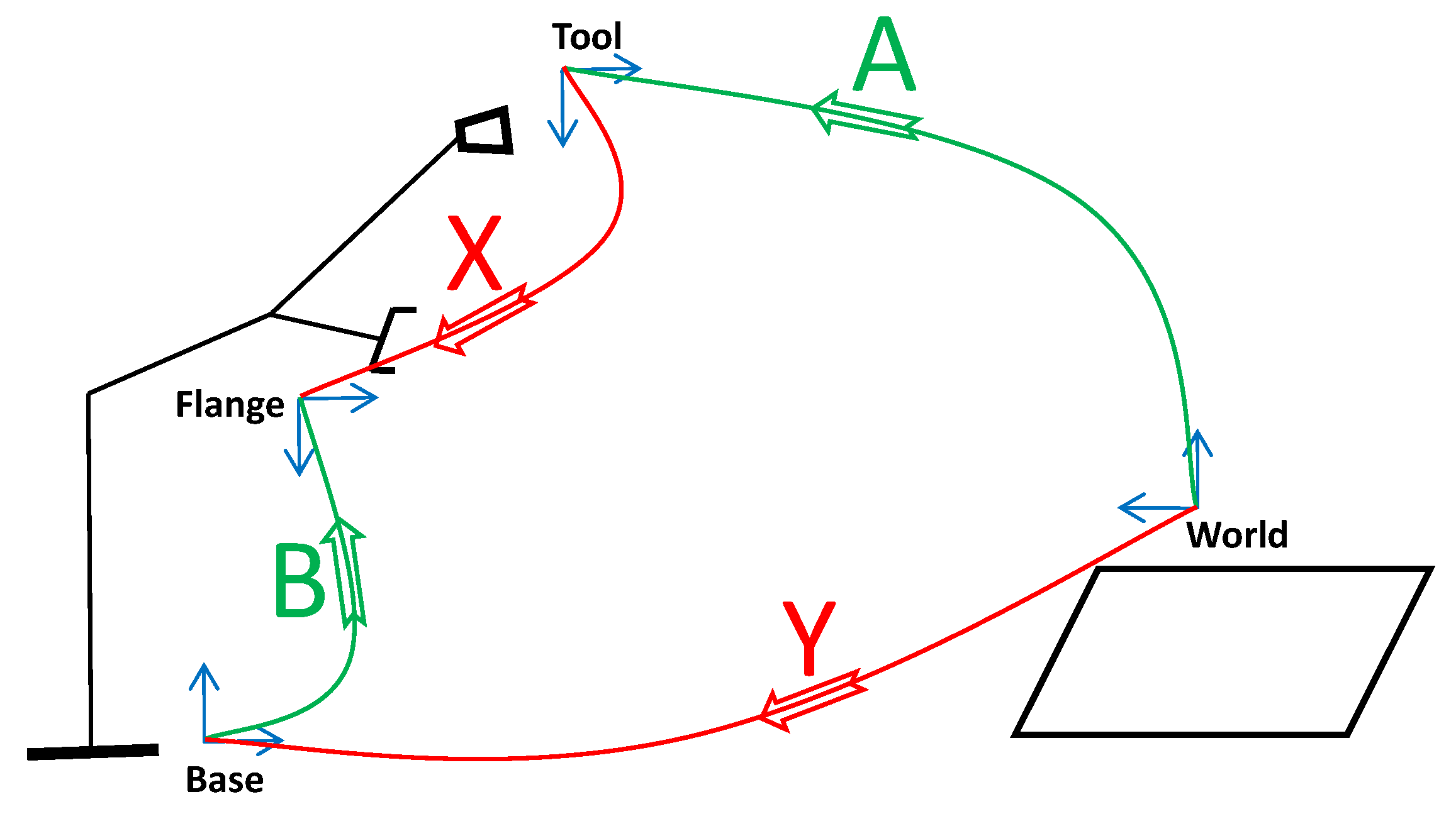
Figure 2.
Encrypting and decrypting color images
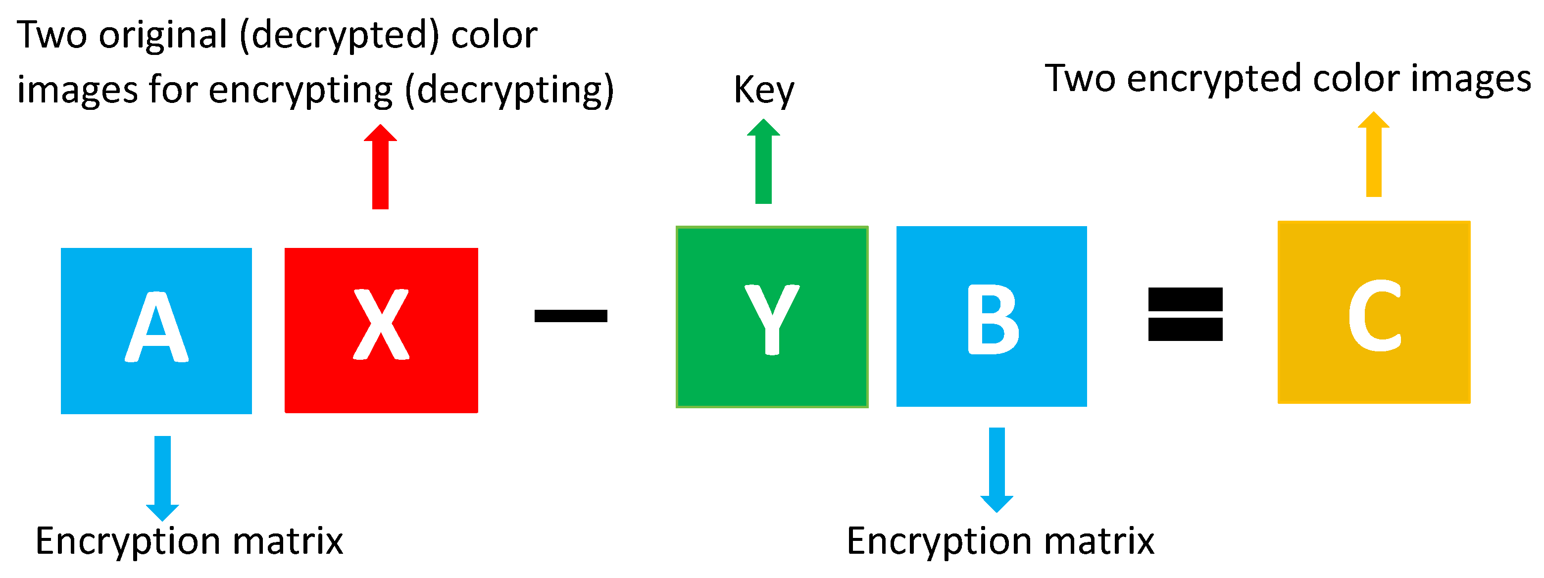
Figure 3.
Core framework of GSE research
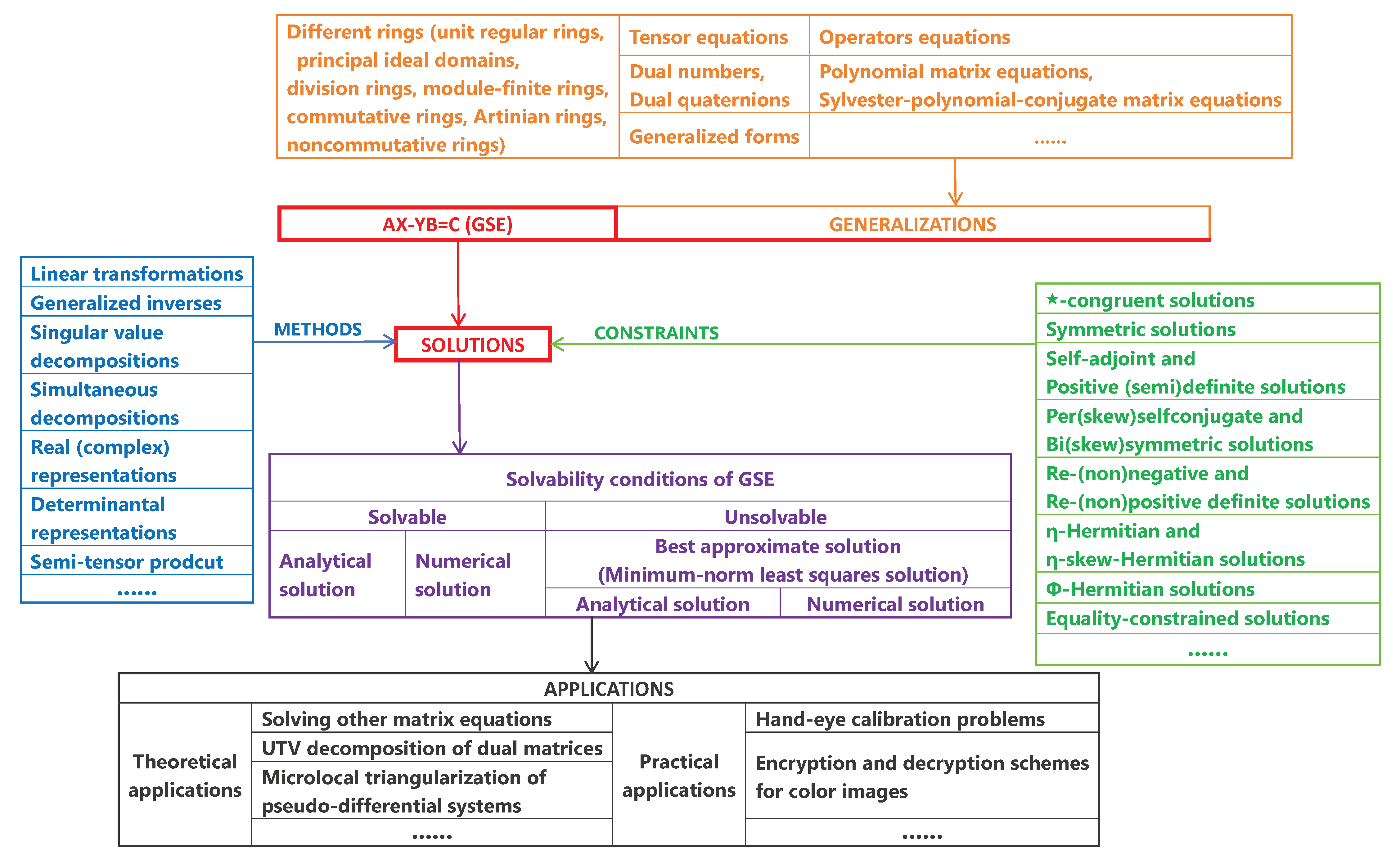
Disclaimer/Publisher’s Note: The statements, opinions and data contained in all publications are solely those of the individual author(s) and contributor(s) and not of MDPI and/or the editor(s). MDPI and/or the editor(s) disclaim responsibility for any injury to people or property resulting from any ideas, methods, instructions or products referred to in the content. |
© 2025 by the authors. Licensee MDPI, Basel, Switzerland. This article is an open access article distributed under the terms and conditions of the Creative Commons Attribution (CC BY) license (http://creativecommons.org/licenses/by/4.0/).
Copyright: This open access article is published under a Creative Commons CC BY 4.0 license, which permit the free download, distribution, and reuse, provided that the author and preprint are cited in any reuse.


