Submitted:
12 August 2025
Posted:
14 August 2025
You are already at the latest version
Abstract
In industrial equipment containing hydraulic lines for power transmission, the lines have boundary conditions defined by components such as pumps, valves, and actuators located at the ends of the lines. Sudden changes in any of the boundary conditions may result in significant pressure/flow dynamics (fluid transients) in the lines that may be detrimental or favorable to the performance of the equipment. Accurate models for line transients are defined by a set of simultaneous partial differential equations. In this paper, analytical solutions to the partial differential equations provide Laplace transform transfer functions applicable to any set of boundary conditions yet to be specified that satisfy the requirements of causality. Analytical solutions from previous publications are reviewed for cases of laminar and turbulent flow for Newtonian and a class of non-Newtonian fluids. When obtaining time domain simulations for specific boundary conditions, complexities associated with the inverse Laplace transform are avoided by using an inverse frequency algorithm. Examples with pumps, valves, and actuators demonstrate the process of coupling equations for components at the ends of a line to get total system transfer functions and then obtaining time domain solutions for outputs-of-interest associated with system inputs and load variations.
Keywords:
fluid transients in smooth circular tubes
; Newtonian fluid
; non-Newtonian fluid
; laminar flow
; turbulent flow
; actuators
; pumps
; valves
; boundary conditions
; water hammer
1. Introduction
Hydraulic power transmission lines are common in industrial equipment. Consider the schematic of a fluid line shown in Figure 1.
The boundary conditions for the line in Figure 1 are defined by the pressure variables and flow rate variables shown on the schematic. Analyses of the fluid transients in a line often focus on variables such as shear stress and pressure at different locations in the line. In this paper, however, the focus is on the effects of the fluid transients interacting with components such as pumps, valves, and actuators at the ends of the line. Such components define the boundary conditions at the ends of a line. By analytically solving the partial differential equations in terms of yet to be specified boundary conditions, it is possible to obtain transfer function equations applicable to any set of boundary conditions that meet the requirements of causality [1].
A survey paper [1] on modeling techniques for fluid transients in smooth circular lines (Figure 1) presents frequency domain analytical solutions for a variety of assumed complexities in the model for the line and fluid properties. Equation (1) is a matrix representation of the equations from this reference for the analytical solution of the ‘dissipative model’ which includes viscosity and heat transfer effects in the model for fluid transients in lines with Newtonian fluids.
In Eq. (1), ‘s’ is the Laplace transform variable, is the propagation operator, and Z(s) is the characteristic impedance. Equation (1) has been proven to be experimentally accurate for laminar mean flow conditions and “over a limited turbulent mean flow range”. The hyperbolic Bessel functions in Eq. (1) can be expressed in terms of infinite order product series for identifying dominant modes, resonant frequencies, and damping ratios [2].
Previous publications document reformulations of Eq. (1) for turbulent flow [3,4] and for a certain class of non-Newtonian fluids [5,6,7,8,9]. A review of the derivation of these reformulations is presented in Appendix A. In all cases, the reformulations fit the normalized small perturbation format shown in Eq. (2).
where
where is the fluid density, is the wave speed, is the internal line radius, and is the pre-transient absolute viscosity. The perturbation variables in Eq. (2) are associated with changes (transients) relative to pre-transient steady-flow conditions. In Eq. (2), the pressure perturbations have been normalized by dividing by the pre-transient steady-flow pressure differential between the ends of the line, . The flow rate perturbations have been normalized by dividing by the pre-transient steady-flow rate through the line, . The normalized Laplace variable, , in Eq. (10) indicates that time has been normalized; is the pre-transient kinematic viscosity.
In Eq. (2), for pre-transient steady-flow Reynolds numbers < 1187.6, the flow is assumed laminar and n=1 and For Reynolds numbers > 1187.6, the pre-transient flow is assumed turbulent; n is an integer between 1 and 10 (based on convergence at relatively high Reynolds numbers) and is based on an empirical friction factor formula for smooth pipe (see Appendix A), i.e.
It is important to note that the transition Reynolds number 1187.6 has been obtained by equating the laminar flow Darcy friction factor equation to the Blasius empirical formula for turbulent flow. Equation (8) is the Oldroyd-B shear stress transfer function for a class of non-Newtonian fluids. For , viscosity decreases (shear thinning) as transient frequencies increase. For , an increase in viscosity occurs as the frequency increases. For , the viscosity is constant corresponding to a Newtonian fluid.
Section 2 of this paper contains examples using Eq. (2) to obtain total system transfer function models when components such as pumps, valves, and actuators are attached to the ends of the line. Since Eq. (2) is applicable to laminar or turbulent pre-transient flows with Newtonian or a certain class of non-Newtonian fluids, it is convenient to reformulate and express Eq. (2) in an all-encompassing simplified format to use for each of the examples, i.e.
It is important to note that for values of n > 1, the terms in Eq. (10) are defined only after raising the matrix in Eq. (2) to the nth power. Obtaining transfer functions for a system with components such as pumps, valves, and actuators interconnected by fluid lines is the focus of Section 2.
Using these infinite order transfer functions in Eq. (10) to generate time domain simulations and important parameters such as resonant frequencies, time constants, and damping ratios is the focus of Section 3. Section 3 of the paper explains how to accurately convert total system transfer functions containing the terms in Eq. (10) to accurate linear finite order equivalent transfer functions containing the dominant modes and the correct DC gain. Having these equivalent transfer functions enables one to perform time domain simulations and analyses without having to decide which terms in infinite series formulations to include, without having to figure out how to revise the series to achieve the correct DC gain [2], without having to deal with the complexities of an inverse Laplace transform [10], and without having to redo each method-of-characteristics numerical solution for each change in boundary conditions [11] associated with components at the ends of the line. A MATLAB mfile is included in Appendix B for implementing the inverse frequency algorithm and generating time domain simulations used in examples in Section 2.
2. Application Examples
There are 4-variables in the 2-equations in Eq. (10): and . Thus, additional equations, considering the requirements of causality, associated with the boundary conditions must be specified to complete the analytical solution for a specified total system. The process of adding additional equations associated with the boundary conditions associated with component hardware is demonstrated in the examples that follow.
2.1. Water Hammer
This example is likely a case where the fluid transients have a detrimental effect on system components. Suppose the pressure at the left end of the line is constant, then . In this case, solving the two equations in Eq. (10) gives
The transfer function is the frequency domain infinite order analytical solution typically used to model the fluid transients (water hammer) due to sudden changes in the flow The transfer function in Eq. (11) can be used to generate a time domain solution for given the time history of . In water hammer studies, a typical assumption is that instantly decreases from the pre-transient flow rate to 0; that is, is a negative step function from 1 to 0 [11].
When working with an infinite order transfer function, it is convenient to first get a finite order approximation for the transfer function. This can be accomplished using product series for hyperbolic and Bessel functions [1,2]; this approach has been proven to be most difficult when it comes to satisfying the low frequency gain associated with steady-state conditions. A more simple and direct approach for getting finite order approximations is by approximating the frequency response of the transfer function over a specified frequency range using an inverse frequency algorithm [3]. A frequency response pertains to the output if the input to the transfer function is a sinewave. Assuming a sinusoidal input to a transfer function, the output will become a sinusoidal function with the same input frequency; however, the output amplitude will either be greater or smaller than the input amplitude depending on the magnitude (dynamic gain) of the transfer function at the input frequency. The frequency response of a transfer function consists of two plots: (1) The magnitude plot representing the dynamic gain as a function of the input frequency, and (2) The phase angle plot resenting the time shift between the input sinewave and the output sinewave as a function of the input frequency. Transfer function approximations must match both parts of the frequency response over a specified range of frequencies. As will be demonstrated, an inverse frequency algorithm achieves this goal.
To generate the water hammer time domain solution for , the recommended first step is to get a frequency response plot of . The second step will be to use an inverse frequency algorithm to get a finite order approximation for the frequency response over a specified range of frequencies (see Section 3). An example of the results using the inverse frequency algorithm is shown in Figure 2, Figure 3 and Figure 4 for a water line 37.23 m in length, with a 22.1 mm diameter, and with a pre-transient Reynolds number of 5600. These line dimensions and pre-transient flow conditions are associated with experimental data [12] used in the verification of the analytical solutions for turbulent flow [3]. The MATLAB mfile for generating Figure 2, Figure 3 and Figure 4, that is also applicable to other transfer functions, is listed in Appendix B.
Referring to the magnitude plots in Figure 2, it is of interest to note that the input specification to the inverse frequency algorithm was to get a match over the normalized frequency range from 10-11 to 8x10⁴; the minimum value 10-11 was chosen to get the DC gain near the correct value of -1 and the maximum value 8x10⁴ chosen to accurately include at least seven 2nd order dominant modes. For purposes of resolution, the minimum normalized frequency shown on the graph is 500 even though 10-11 was used in the algorithm. Also, note that the first three normalized resonant frequencies and peak values have been accurately identified with data tips. For example, at the normalized resonant frequency of 5689, the sinusoidal pressure amplitude amplification is The order of the transfer function approximation needed to be 19 to get a good fit over the specified frequency range. The mfile generates eigenvalues, damping ratios, and time constants.
An accurate match of the phase plots over the frequency range is confirmed in Figure 3.
As shown in detail in Appendix B, the normalized water hammer pressure time history shown in Figure 4 was obtained by assuming a nearly instant valve closure input to the transfer function approximation for 5 different values of ‘n’. A comparison of the plots reveals that n = 1 would be sufficient for this low level of turbulence. As shown in Figure 4, the water hammer initial pressure surge following valve closure peaks at about 150 = 4.155x10⁵ N/m2.
2.2. Pump and Valve on the Ends of the Line
Consider the schematic in Figure 5 of a line with a pump and a valve on the ends of the line. For this example, the passage area through the valve may be a function of time. For the pump, the output flow or pressure may be a function of time.
Assume the flow through the valve is defined by the orifice equation with variable area and coefficient The orifice equation that models forward or reverse flow is
Linearizing Eq. (13) about the pre-transient steady flow conditions gives
To maintain consistency with the line transfer function equations, the pressure and flow variables are normalized by the equation for pre-transient steady flow through the line, i.e.
The dimensionless parameter q represents the ratio of the pre-transient valve resistance to the line steady-flow resistance .
The two equations in Eq. (10) and Eq. (15) contain 6-normalized perturbation variables: , , , , and , i.e.
Thus, to complete the solution, one or more of the variables must be designated as input(s) and/or additional equations added. Consider the examples in the following section.
2.2.1. Constant Flow from Pump with Changing Valve Area
For example, suppose is designated to be an input, the pump has a fixed displacement with a constant output flow, and the value output pressure is constant, If the output of interest is , then Eq.’s (16-18) simplify to give the desired transfer function equation, i.e.
Time domain plots of for different valve area changes can be generated once the transfer function in Eq. (19) is approximated by a ratio of finite order rational polynomials.
2.2.2. Constant Valve Area with Changing Flow from a Variable Displacement Pump
In this example, fluid transients are desired and likely improve the performance of the system. Pumps are used to force fluids into downhole fissures in rock formations for oil and gas production. Pulsating flow rates from variable displacement pumps at resonant frequencies of the pressure transients in lines can enhance the performance of the system significantly. The transfer function for perturbations in the downhole flow rate can be obtained from Eq.’s (16-18). Assuming is specified to be an oscillating input and and , Eq.’s (16-18) simplify to
As with previous transfer functions derived in this section, the transfer function in Eq. (20) is infinite order. As shown in Figure 6, a frequency response of this transfer function with q = 10 reveals that the first mode resonant frequency occurs at a normalized frequency of 5689 with dynamic gain 21 dB. Thus, for a sinusoidal flow rate out of the pump at this resonant frequency superimposed on a mean flow, the amplitude of the sinusoidal output flow rate perturbations at the end of the line will be times larger than the input amplitude. The results and accuracy of the inverse frequency algorithm are also shown in Figure 6; having an approximation for the transfer function enables one to generate time domain plots of for any other pump output flow rate specifications such as pulses, etc. It is important to note that the same mfile was used to generate Figure 6; the only changes in the mfile are the equation for the transfer function and the label on the y-axis of the graph.
2.3. Rotary Actuator Controlled by a Variable Displacement Pump
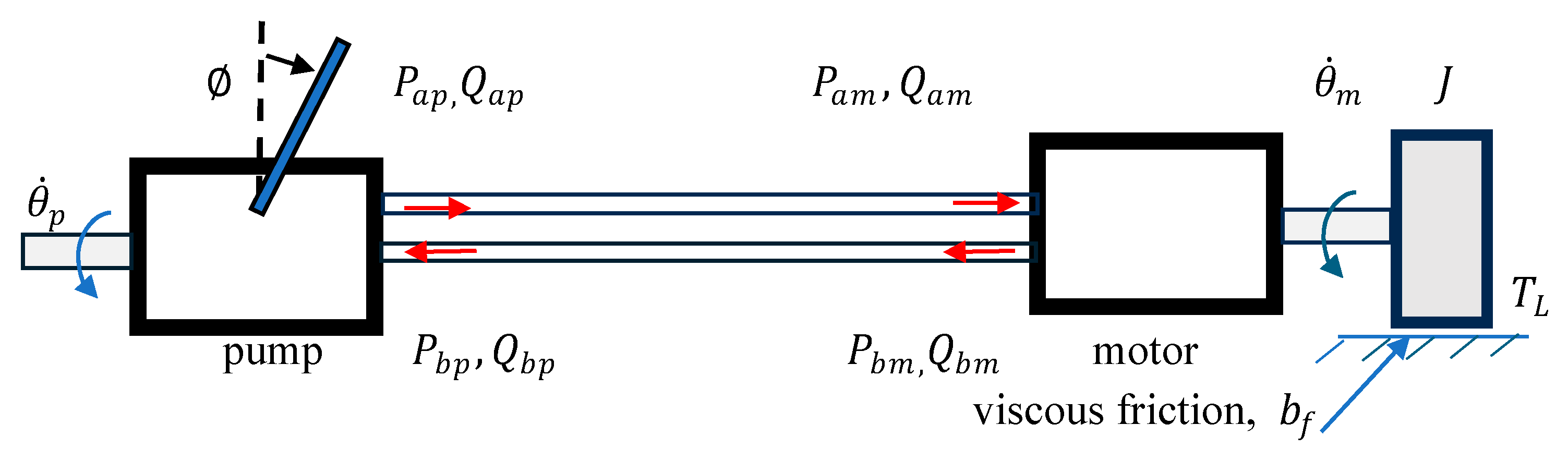
A variable displacement pump is used to power and control the speed of a hydraulic motor (rotary actuator) [13]. A schematic of the system is shown Figure 7.
The rotation speed, of the pump input shaft is assumed constant. The rotation direction and speed of the motor is determined by the direction and magnitude of the flow in the lines which is indirectly determined by the pump displacement control lever. The significance of the fluid dynamics and flow losses in the lines are functions of the length and diameter of the lines and the frequencies of the input and the load torque . The variables labeled on the schematic indicate the positive direction of the flows corresponding to counterclockwise rotation of the motor and clockwise torque representing the load on the motor shaft opposing the rotation of the motor. Most likely, it would be desirable for the input frequencies from the pump and/or load torque to be well below the resonant frequencies of the total system which are defined by the fluid transients coupled with the load dynamics. The following derivation formulates the transfer function for the total system which provides the eigenvalue frequencies that should be avoided.
The pump displacement is proportional to the swash plate angle ; thus, the flow from the pump in terms of the pump shaft angular velocity is
The flow through the motor is proportional to the motor displacement , i.e.
The torque equation on the motor shaft is
where is the rotational inertia of the load, is a viscous damping coefficient, and is the motor torque coefficient.
Laplace transforming Eq.’s (20-22) and then rewriting in small perturbation normalized format gives
Using Eq. (10) line ‘a’ and for line ‘b’ (see Figure 7), we get the normalized perturbation equations for the fluid transients in the lines, i.e.
Assuming no leakage, we can write
In Eq.’s (24-30 ), there are two input variables, and and there are nine unknowns: , ,, , , and . Thus, it is possible to solve for the transfer functions for any of the unknown variables. For example, suppose that the output-of-interest is the perturbation in the motor speed ; this variable can be rewritten in normalized Laplace format, i.e.
Eliminating all of the unknowns except from Eq.’s (24-30) gives
There are two transfer functions in Eq. (32) for the inputs and . Thus, the time history of the rotational speed of the motor, considering the fluid transients, can be obtained for any input specifications once the transfer functions have been approximated by ratios of finite order polynomials.
3. Suggestions for Approximating Infinite Order Transfer Functions Using an Inverse Frequency Algorithm
The MATLAB inverse frequency command is as follows:
[NumCoeffs,DenCoeffs]=invfreqs(FreqResp,Freq,NumOrder,DenOrder,Wt)
where ‘FreqResp’ are the complex frequency response values at the frequencies ‘Freq’, ‘NumOrder’ and ‘DenOrder’ are the desired orders of the polynomials in the transfer function approximation, and ‘Wt’ are optional weighting coefficients. A maximum frequency and a minimum frequency are used to generate the values ‘Freq’. I use 1000 points per decade and all weighting terms of one. Assigning values to the inputs in the ‘invfreqs’ function is a trial-and-error process. The following suggestions are recommended:
1. The first step is to estimate a minimum value and a maximum value that define a frequency range for a frequency response of the total system model such as in Eq.’s (11), (19), (20), and (32). Examination may reveal the presence of resonant frequencies and the low frequency requirements for an accurate DC gain. Change the minimum and maximum values until an acceptable frequency range is achieved. Consider the following statements used to generate the frequencies ‘Freq’ in your specified frequency range for the curve fit approximation.
wmin=.00001;wmax=120000; % Defines the frequency range for the curve fit
nd=ceil(log10(wmax)-log10(wmin)); %Determines the number of decades in the frequency range and rounds up to the next integer
w=logspace(log10(wmin),log10(wmax),1000*nd); %Generates at least 1000 points per decade to be used when getting the curve fit approximation
2. If resonant frequencies exist, then it is possible to estimate the order of the transfer function that will be required to accurately curve fit the response out to an upper frequency; at least 2 orders are required for each resonant peak and possibly additional orders for first order modes that are not apparent from examining the frequency response. To determine the number of dominant modes to include, keep increasing the order until there is little change in the eigenvalues and the time response.
dorder=23; % Desired order for the denominator of the transfer function
3. For a specific desired upper frequency, it is better to start with a lower order trial value and work up to a higher order with each trial to obtain an accurate fit out to that upper frequency
4. The order of the numerator should always be one less than the order of the denominator.
norder=dorder-1; % Desired order for the numerator of the transfer function
5. With each attempt, the DC gain of the transfer function should be checked. There will always be a trade off in accuracy at the lower and upper frequencies. The lower frequency should be decreased until the desired DC gain is achieved to the desired accuracy.
6. To generate time domain plots, it is important to note that the coefficients of the transfer function approximation are stored in memory. Simply create a transfer function with these coefficients and then use whatever linear simulation function is appropriate for a specific input function.
G=tf(NumCoeffs,DenCoeffs); % Creates the transfer function
Dcgain=dcgain(G) % Calculates the low frequency gain of the transfer function
step(G) % Generates a plot for a unit step input to the transfer function
The complete MATLAB mfile used to generate the approximation and time domain plots in Figure 2, Figure 3 and Figure 4 is listed in Appendix B.
4. Discussion
Accurate models for fluid transients in lines are defined by a set of simultaneous partial differential equations. As demonstrated in Appendix A, the analytical solution to these partial differential equations is obtained without having to specify specific details about components at the ends of the line. This is very desirable and provides significant versatilities to the analysis of the interaction of fluid transients with different end-of-line components. The analytical solution is applicable to either laminar or turbulent pre-transient flow for Newtonian [3] and a specific class of non-Newtonian fluids [9]. Compared to numerical solution approaches, such as the method-of-characteristics, the analytical solution to the partial differential equations does not have to be repeated with each end-of-the-line component design change and/or with each change in the external inputs.
Components at the ends of the line are typically modeled with ordinary differential equations and/or algebraic equations. These equations define the boundary conditions for a line which must satisfy causality requirements. Coupling the transfer functions for a line with equations for the components on the ends of the line to get a total system model, enables the generation of (1) time domain plots of system outputs-of-interest using linear or nonlinear simulation algorithms, (2) frequency response analyses, (3) computation of eigenvalue time constants, resonant frequencies, and damping ratios, and (4) models for controller designs for optimizing total system performance. Examples of coupling the analytical model for the line transients to equations for various fluid power components have been presented in Section 2. In some cases, the fluid transients are undesirable and should be avoided by operating the system at frequencies well below the system resonant frequencies. A waterhammer example was formulated and MATLAB code used to generate transfer function approximations and time domain simulations demonstrating the detrimental effects of fluid transients in lines. In a different example of a downhole fracking system, performance was enhanced by oscillating the flow rate input to the line at the first mode resonant frequency of the total system transfer function.
As demonstrated with the examples, once the boundary condition equations have been coupled with the Laplace transform solution to the fluid transient partial differential equations, a total system transfer function is achieved. These solutions have been derived using the Laplace transform which typically has not been a favorable approach due to the complexities of getting inverse Laplace transforms of infinite series formulations. In this paper, however, the complexities associated with the inverse Laplace transform are avoided by using an inverse frequency algorithm. Tips on using the inverse frequency algorithm are provided in Section 3; these tips are based on years of experience of trial-and-error selection of the frequency range and order of the polynomials in the transfer function approximation.
A MATLAB mfile is provided in Appendix B. The specific parameters and transfer function in the mfile pertain to the examples in Section 2.1 and Section 2.2.2. This mfile can be used with any transfer function formulated with the fluid transient equations and component equations with proper adjustment of the parameters as suggested in Section 3. Comment statements have been added to the MATLAB code to simplify the use of the mfile for other system transfer functions. The mfile contains many lines of code; however, it is important to note that the majority of the code pertains to the generation of output plots with appropriate labeling some of which may not be needed.
Funding
This research received no external funding.
Conflicts of Interest
The author declares no conflicts of interest.
Appendix A. Analytical Solution to the Partial Differential Equations Considering Potentially Non-Newtonian Turbulent Flow Conditions
Appendix A.1. Newtonian Fluids
The closed form Newtonian analytical model for laminar flow transient perturbations in circular lines has been documented, experimentally verified, and used successfully for more than 50 years [1]. The primary objective of this Appendix is to extend this model for transient perturbations in non-Newtonian fluids and then extend it further for turbulent flow. The partial differential equations for the momentum, continuity, energy, and state for the dissipative model for laminar flow in a horizontal smooth line are listed in Eq.’s (A1-A3) [1]. The simplified isothermal version of these equations for compressible liquids with only -direction axial flow are as follows
The axial velocity is a function of and ; is the pressure which is assumed to be uniform at any specific ; is the stress tensor as a function of and ; is the pre-transient fluid density, and is the equivalent bulk modulus of the fluid which is a function of the elasticity of the line walls and can be adapted to include the effects of entrained gas.
For Newtonian fluids and laminar flow, the well-known frequency domain solution to Eq.’s (A1-A3) in terms of the normalized Laplace variable is shown in Eq.’s (A4-A9) [1]. The details of this solution will be repeated in this appendix but with the addition of the non-Newtonian terms [4,5,6,7] and the impedance effects of turbulence [3]. This solution can be expressed in terms of normalized frequency using
where
Appendix A.2. Extension of the Newtonian Analytical Model to Non-Newtonian Fluids
The well-known and widely accepted derivation for the Newtonian analytical model in Eq. (A4) is repeated here but, as mentioned above, expanded to include the Oldroyd-B stress tensor model [5,6,7,8,9]. Combining Eq.’s (A2) and (A3) gives
Laplace transforming Eq.’s (A1) and (A10) assuming zero initial conditions and normalizing gives
Substituting Eq. (3) for the Oldroyd-B shear stress model into Eq. (A11) gives
Rearranging and collecting the terms in Eq. (A13) gives
or
where
Eq. (A15) is a Bessel equation with solution
where
The function is not a function of and will be defined by the boundary conditions at the ends of the line. Using Eq.’s (A16) and (A18), the solution for can be written, i.e.
Considering that there is no slip at , Eq. (A20) gives
Thus,
Substituting Eq. (A22) into Eq. (A20) gives an equation for the velocity as a function of , , and , i.e.
At this point in the derivation, the assumption will be made that the flow passage is a circular pipe with radius . Since the boundary conditions at the ends of the line will be in terms of the flow rates and pressures, it is convenient to compute the average velocity. Multiplying Eq. (A23) by and then integrating, and dividing by gives
where
Solving for in Eq. (A12) and then taking the derivative with respect to gives
Taking the 2nd derivative of Eq. (A25) with respect to gives
From Eq. (A22)
Substituting Eq. (A27) into Eq. (A29) gives
Substituting Eq. (A28) into Eq. (A30) gives
Rearranging Eq. (A31) gives the following equation
where
The solution to Eq. (A32) is
where and are determined by the boundary conditions at the ends of the line defined by the flow rates and pressures. Using Eq. (A25), we get
The equations for the pressures require the use of Eq. (A12) and the derivative of Eq. (A25), i.e.
Thus,
From Eq. (A36)
From Eq. (A40)
Thus, substituting Eq. (A42) and Eq. (A43) into Eq. (A37) and Eq. (A41) gives
or
where
Equation (A45) represents the non-Newtonian version of Eq. (A4). It is of interest to note that Eq. (A45) is identical to Eq. (A4) except for the inclusion of the Oldroyd-B shear stress terms in and in the parameter in Eq. (A48). Also, Eq.’s (A46) and (A47) are identical in form to Eq.’s (A7) and (A6), respectively. Setting makes ; so, Eq. (A45) for non-Newtonian becomes identical to Eq. (A4) for Newtonian.
Appendix A.3. Extension to Pre-Transient Turbulent Flow
For Newtonian fluid, Eq. (A4) was extended to a model for pre-transient turbulent flow [3]. Since Eq. (A45) is identical to Eq. (A4) except for the inclusion of the non-Newtonian shear stress parameters in the parameters and , the extension of Eq. (A4) to turbulent flow is applicable to the non-Newtonian model in Eq. (A45). The extension to pre-transient turbulent flow is summarized here in order to clarify the derivations of equations for pre-transient turbulent normalized shear stress and normalized velocity which are included in this Appendix.
The pre-transient turbulent flow model is based on using the analytical model in Eq. (A45) in series with a lumped resistance sized so that the resulting model for the line has the same steady flow resistance of a smooth line with pre-transient turbulent flow [3]. To potentially improve the accuracy of the model for relatively large Reynolds numbers, the resistance is distributed along the line by dividing the line into n-sections. The schematic for such a multi-sectioned model is shown in Figure A1 where are intermediate pressures and flows.
Figure A1.
Line of length L with a lumped resistance at the end of each segment of length L/n.
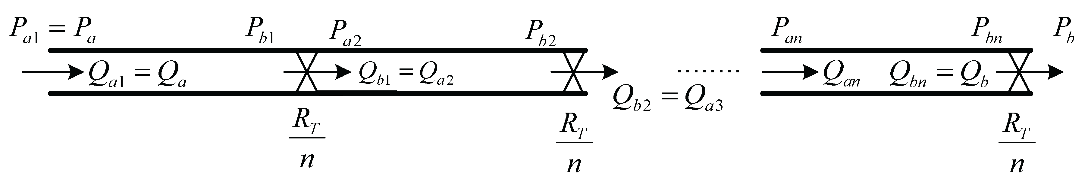
The Blasius empirical model for the Darcy friction factor for smooth lines is utilized to establish the turbulent flow resistance . For Reynolds numbers up to 200,000 [3,4] in smooth lines with steady flow , the corresponding pressure differential between the ends of a horizontal line is
where
Denoting the steady flow laminar resistance by , it can be shown that the additional resistance needed to match the total resistance for turbulent flow is given by
Using normalized perturbation variables representing pressure and flow changes from the pre-transient turbulent level, the resulting model for the transients in the line is [3].
where
and
It has been demonstrated that Eq. (A52) for Newtonian fluids gives good agreement with water hammer experimental data and MOC solutions with values of n from 1 to 10 and Reynolds numbers up to 15,800 [3]. It has been demonstrated for water hammer simulations, a value of 10 is sufficient for decay rate convergence for Reynolds numbers out to 200,000 [4].
Referring to Eq. (A52), it can be shown that if ; this is the transition Reynolds number for which the Blasius and laminar flow friction factors are identical. It is also important to note that for =1 and RT = 0, Eq. (A52) gives the solution for pre-transient laminar flow in a horizontal smooth line.
Appendix B. MATLAB Mfile
The following MATLAB mfile pertains to the waterhammer example in Section 2.1. The program will work for other transfer functions by changing the definition of ‘H’ in the internal function ‘TransferFunctionTF’ at the end of the code. Note, for other transfer functions, it may be necessary to make changes in lines 6-8 of the code.
function TransferFunctionApproximation
warning off
format shortg
% Required inputs; you will have to guess the order, wmax, and wmin at first until
% you see the frequency response and decipher the necessary frequency range
dorder=19;wmin=1e-11;wmax=80000;wminplot=500;wmaxplot=1.25*wmax;
den=999.11;a=1319;r=0.01105;L=37.23;kvis=1.1839e-6;
Rn=5600; % you can specify Rn and then solve for Qe
Qe=kvis*pi*r*Rn/2 % you can specify Qe and then solve for Rn
absvis=den*kvis;
Dn=kvis*L/(a*r^2)
if Rn>=1187.6
n=1; %Desired number of segments in turbulence model.
%May need to be increased for larger % values of Dn
Pe=0.2414*(den^0.75)*(absvis^0.25)*L*(Qe^1.75)/(2*r)^4.75
else
n=1;
Pe=8*absvis*L/(pi*r^4)
end
norder=dorder-1;
nd=ceil(log10(wmax)-log10(wmin)); %Determines the number of decades in the frequency
% range and rounds up to the next integer
w=logspace(log10(wmin),log10(wmax),1000*nd); %Generates at least 1000 points per decade
Lw=length(w);
for k=1:Lw
s(k)=w(k)*1i;
[H(k)]=TransferFunctionTF(s(k));
end
wt=ones(1,Lw); %weighting terms for curve fit
[numa,dena]=invfreqs(H,w,norder,dorder,wt,100); %curve fitting with 100 attempts if necessary
Gapprox=tf(numa,dena); %linear transfer function approximation from curve fitting frequency response
damp(Gapprox) %gives eigenvalues of the transfer function
% comparing the dcgain of the approximation and the original transfer functions
DCGain=dcgain(Gapprox)
% helps to determine if wmin was low enough
%
% Generate Freq. Resp. plots to determine the accuracy of curve fit.
if wminplot>=wmaxplot, error(‘wmin is too small; very low non-resonant peaks are messing up the calcultions. Increase wmin and try again.’),end;
ndp=ceil(log10(wmaxplot)-log10(wminplot)); %Determines the number of decades in the plotting
%frequency range and rounds up to the next integer
wp=logspace(log10(wminplot),log10(wmaxplot),500*ndp); %Generates at least 500 points per %decade for the plots
Lwp=length(wp);
Hc=freqs(numa,dena,wp); %generates frequency response of the computed transfer function
MHc=20*log10(abs(Hc)); %magnitudes of the frequency response in dB
AHc=angle(Hc)*180/pi; %angles of the frequency response in degrees
clear H s
% recompute the original function with same frequencies used for the transfer function approximation
for k=1:Lwp
s(k)=wp(k)*1i;
[H(k)]=TransferFunctionTF(s(k));
end
MH=20*log10(abs(H));
AH=angle(H)*180/pi;
figure(1)
semilogx(wp,AH,’k’,wp,AHc,’r:‘,’LineWidth’,2)
title(‘Phase Angle Comparison Plots. Rn=5600’)
xlabel(‘Normalized frequency \omega/\omega_v ‘)
ylabel(‘Phase Angle, degrees’)
legend(‘Original function’,’Approximation’,’Location’,’Best’)
grid on
grid minor
figure(2)
semilogx(wp,MH,’k’,wp,MHc,’r:‘,’LineWidth’,2)
xlabel(‘Normalized frequency \omega/\omega_v ‘)
ylabel(‘Normalized transfer function magnitude, ( \DeltaP_b/P_e)/ ( \DeltaQ_b/Q_e) dB’)
%ylabel(‘Normalized transfer function magnitude, ( \DeltaQ_b/Q_e)/ ( \DeltaQ_a/Q_e) dB’)
legend(‘Original function’,’Approximation’,’Location’,’Best’)
title(‘Magnitude Comparison Plots, Rn=5600’)
grid on
grid minor
Cv=1; % 0 < Cv < 1 with 1 corresponding to 100% valve closure
Vct=0.008; % closure time in seconds if 100% closure
VCt=Vct*Cv; % Valve partially close time in seconds
% the negative sign is associated with the valve closing which is a negative change in flow
[ynorm,tnorm]=step(-Cv*Gapprox,0.014);
% to shorten the normalized simulation time to FT use step(Gapprox,FT)
t=tnorm*r^2/kvis; % unnormalized time s
for nt=1:length(t) % generate shaped valve closing as a function of time in sec.
if t(nt)<=VCt
u(nt)=.5+0.5*cos(pi*(t(nt)/VCt-1));end
if t(nt)>VCt
u(nt)=1;end
end
u=Cv*u; % 0 < Cv <=1 for partial valve closing
Pnorm=lsim(Gapprox,-u,tnorm);
figure(3)
plot(tnorm*r^2/kvis,Pnorm,’r’,’LineWidth’,2) % plot using normalized pressure and un-normalized time
grid
xlabel(‘time, sec.’)
ylabel(‘Normalized Pressure at Valve, \DeltaPv/Pe’)
title(‘Rn=5,600, L=37.23 m, Dn=2.737e-4, Pe=2,770 N/m^2’)
hold
den=999.11;a=1319;r=0.01105;L=37.23;Vo=0.30;
%__________________________________________________________________________________
n=2;
norder=dorder-1;
nd=ceil(log10(wmax)-log10(wmin)); %Determines the number of decades in the frequency % range and rounds up to the next integer
w=logspace(log10(wmin),log10(wmax),1000*nd); %Generates at least 1000 points per decade
Lw=length(w);
for k=1:Lw
s(k)=w(k)*1i;
[H(k)]=TransferFunctionTF(s(k));
end
wt=ones(1,Lw); % weighting terms for curve fit
[numa,dena]=invfreqs(H,w,norder,dorder,wt,100); % curve fitting with 100 attempts if necessary
Gapprox=tf(numa,dena); % linear transfer function approximation from curve fitting the
% frequency response
damp(Gapprox) %gives eigenvalues of the transfer function
DCGain=dcgain(Gapprox) % comparing the dcgain of the approximation and the original %transfer functions
% helps to determine if wmin was low enough
Pnorm=lsim(Gapprox,-u,tnorm);
figure(3)
plot(tnorm*r^2/kvis,Pnorm,’k:‘,’LineWidth’,2) % plot using normalized pressure and
%un-normalized time
%__________________________________________________________________________________
n=3;
norder=dorder-1;
nd=ceil(log10(wmax)-log10(wmin)); %Determines the number of decades in the frequency %range and rounds up to the next integer
w=logspace(log10(wmin),log10(wmax),1000*nd); %Generates at least 1000 points per decade
Lw=length(w);
for k=1:Lw
s(k)=w(k)*1i;
[H(k)]=TransferFunctionTF(s(k));
end
wt=ones(1,Lw); %weighting terms for curve fit
[numa,dena]=invfreqs(H,w,norder,dorder,wt,100); %curve fitting with 100 attempts if necessary
Gapprox=tf(numa,dena); %linear transfer function approximation from curve fitting frequency %response
damp(Gapprox) %gives eigenvalues of the transfer function
DCGain=dcgain(Gapprox) % comparing the dcgain of the approximation and the original %transfer functions; helps to determine if wmin was low enough
Pnorm=lsim(Gapprox,-u,tnorm);
figure(3)
plot(tnorm*r^2/kvis,Pnorm,’r-.’,’LineWidth’,2) % plot using normalized pressure and
%un-normalized time
%__________________________________________________________________________________
n=4;
norder=dorder-1;
nd=ceil(log10(wmax)-log10(wmin)); %Determines the number of decades in the frequency %range and rounds up to the next integer
w=logspace(log10(wmin),log10(wmax),1000*nd); %Generates at least 1000 points per decade
Lw=length(w);
for k=1:Lw
s(k)=w(k)*1i;
[H(k)]=TransferFunctionTF(s(k));
end
wt=ones(1,Lw); %weighting terms for curve fit
[numa,dena]=invfreqs(H,w,norder,dorder,wt,100); %curve fitting with 100 attempts if necessary
Gapprox=tf(numa,dena); %linear transfer function approximation from curve fitting frequency %response
damp(Gapprox) %gives eigenvalues of the transfer function
DCGain=dcgain(Gapprox) % comparing the dcgain of the approximation and the original %transfer functions; helps to determine if wmin was low enough
ynorm=step(-Cv*Gapprox,tnorm); % to shorten the normalized simulation time to FT
% the negative sign is associated with the valve closing which is a negative change in flow
%step(Gapprox,FT)
Pnorm=lsim(Gapprox,-u,tnorm);
figure(3)
plot(tnorm*r^2/kvis,Pnorm,’k--‘,’LineWidth’,2) % plot using normalized pressure and
%un-normalized time
%__________________________________________________________________________________
n=5;
norder=dorder-1;
nd=ceil(log10(wmax)-log10(wmin)); %Determines the number of decades in the frequency %range and rounds up to the next integer
w=logspace(log10(wmin),log10(wmax),1000*nd); %Generates at least 1000 points per decade
Lw=length(w);
for k=1:Lw
s(k)=w(k)*1i;
[H(k)]=TransferFunctionTF(s(k));
end
wt=ones(1,Lw); %weighting terms for curve fit
[numa,dena]=invfreqs(H,w,norder,dorder,wt,100); %curve fitting with 100 attempts if necessary
Gapprox=tf(numa,dena); %linear transfer function approximation from curve fitting frequency %response
damp(Gapprox) %gives eigenvalues of the transfer function
DCGain=dcgain(Gapprox) % comparing the dcgain of the approximation and the original %transfer functions
% helps to determine if wmin was low enough
%
Pnorm=lsim(Gapprox,-u,tnorm);
figure(3)
plot(tnorm*r^2/kvis,Pnorm,’b’,’LineWidth’,2) % plot using normalized pressure and
%un-normalized time
legend(‘n = 1’,’n = 2’,’n = 3’,’n = 4’,’n = 5’)
hold off
Dn
Pe
function [H]=TransferFunctionTF( s ) % H is the transfer function to be approximated
B=2*besselj(1,j*sqrt(s))/(j*sqrt(s).*besselj(0,j*sqrt(s)));
sqr=sqrt(1-B);
RTOZ=0;g=Dn*s/sqr; %This is the case for laminar flow, Rn<1187.6
if Rn>=1187.6
RTOZ=Dn*sqr*(0.039544*Rn^0.75-8);
g=Dn*s/(n*sqr); % gamma
end
W(1,1)=cosh(g)+RTOZ*sinh(g)/n;
W(1,2)=-(sinh(g)+RTOZ*cosh(g)/n)/(8*Dn*sqr+RTOZ);
W(2,1)=-(8*Dn*sqr+RTOZ)*sinh(g);
W(2,2)=cosh(g);
X=W^n;
% X(i,j) corresponds to aij in the paper
H= X(1,2)/X(2,2); % waterhammer transfer function in Eq. (12)
% H=(X(1,2)*X(2,1)-X(1,1)*X(2,2))/(10*X(2,1)-X(1,1));%flow gain transfer function, Eq. (20)
end
end
References
- Goodson, R.E.; Leonard, R.G. A Survey of Modeling Techniques for Fluid Line Transients. ASME J. Basic Eng. 1971, 94, 474–482. [Google Scholar] [CrossRef]
- Healey, A.J.; Hullender, D.A. State Variable Representation of Modal Approximation For Fluid Transmission Line Models. Special publication of the ASME J. of Dynamic Systems, Measurement and Control, p 57-71, 1981.
- Hullender, D. Alternative Approach to Modeling Transients in Smooth Pipe with Low Turbulent Flow. ASME J. of Fluids Eng. 2016, 138, n12. [Google Scholar] [CrossRef]
- Hullender, D. Water Hammer Peak Pressures and Decay Rates of Transients in Smooth Lines with Turbulent Flow. ASME J Fluids Eng. 2018, 140, n6. [Google Scholar] [CrossRef]
- Bird, R.B.; Armstrong, R.C. and Hassager, O., Dynamics of Polymeric Liquids, 2nd ed., Vol. 1, Wiley, NY, Chapter 2, 1987.
- Oldroyd, J.G. Non-Newtonian effects in steady motion of some idealized elastic-viscous liquids. Proc. R. Soc. A 1958, 245, 278–297. [Google Scholar]
- Oldroyd, J.G. On the formulation of rheological equations of state. Proc. R. Soc. A 1950, 200, 523–541. [Google Scholar]
- McGinty, S.; McKee, S.; McDermott, R. Analytic Solutions of Newtonian and Non-Newtonian Pipe Flows Subject to a General Time-Dependent Pressure Gradient. J. Non-Newtonian Fluid Mech 2009, 162, 54–77. [Google Scholar] [CrossRef]
- Hullender, D. Analytical non-Newtonian Oldroyd-B transient model for pre-transient turbulent flow in smooth circular lines. ASME J. Fluids Eng. 2019, 141, n2. [Google Scholar] [CrossRef]
- Urbanowicz, K.; Bergant, A.; Grzejda, R.; Stosizk, M. About Inverse Laplace Transform of a Dynamic Viscosity Function. Materials 2022, 15, 4364. [Google Scholar] [CrossRef] [PubMed]
- Bergant, A.; Zlatko, R.; Urbanowicz, K. Analytical, Numerical 1D and 3D Water Hammer Investigations in a Simple Pipeline Apparatus, 2025, Stojniski vestnik J. Mechanical Engineering, v 71 n 5-6. [CrossRef]
- Bergant, A.; Simpson, A.R.; Vitkovsk, J. Developments in Unsteady Pipe Flow Friction Modelling. ASCE J. Hydraulic Res. 2001, 39, 249–257. [Google Scholar] [CrossRef]
- Blackburn, JF; Reethof, G; Shearer, JL, Fluid Power Control, 1960, The M.I.T. Press, Lib. of Congress Catalog No. 59-6759, p 499-508, Cambridge, Mass.
- Vıtkovsky, J.P.; Lee, P.J.; Zecchin, A.C.; Simpson, A.R.; Lambert, M.F. Head-and Flow-Based Formulations for Frequency Domain Analysis of Fluid Transients in Arbitrary Pipe Networks. ASCE J. Hydraul. Eng. 2011, 137, 556–568. [Google Scholar] [CrossRef]
Figure 1.
Schematic of a fluid transmission line with the input and output variables.

Figure 2.
Magnitude comparison of the frequency response of the inverse frequency linear transfer function approximation with the exact frequency response of the water hammer transfer function in Eq. (12) for turbulent flow conditions.
Figure 2.
Magnitude comparison of the frequency response of the inverse frequency linear transfer function approximation with the exact frequency response of the water hammer transfer function in Eq. (12) for turbulent flow conditions.
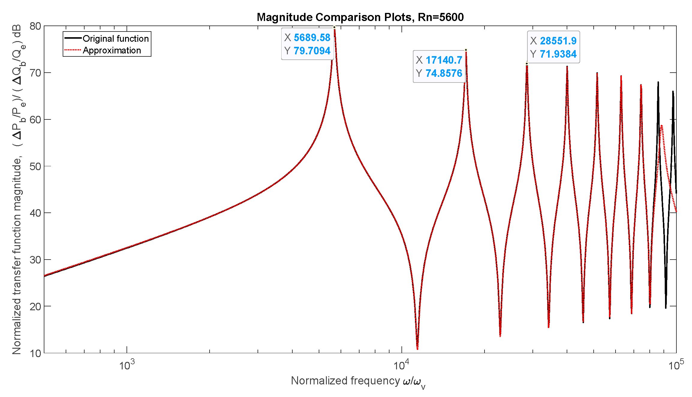
Figure 3.
Phase angle comparison of the inverse frequency response approximation with the exact frequency response of the water hammer transfer function in Eq. (12).
Figure 3.
Phase angle comparison of the inverse frequency response approximation with the exact frequency response of the water hammer transfer function in Eq. (12).
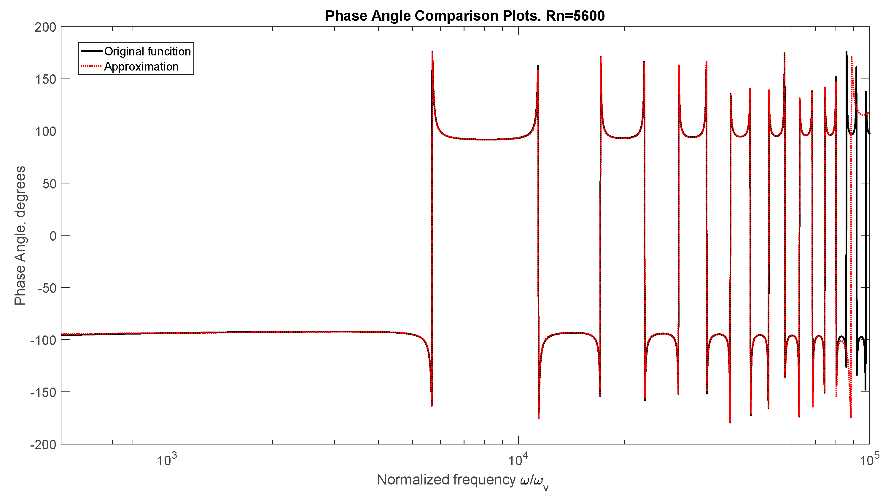
Figure 4.
Normalized pressure upstream of the value following valve closure demonstrating the pressure surge and wave frequency in the line and demonstrating the insensitivity to the number ‘n’ for this relatively low level of turbulence.
Figure 4.
Normalized pressure upstream of the value following valve closure demonstrating the pressure surge and wave frequency in the line and demonstrating the insensitivity to the number ‘n’ for this relatively low level of turbulence.
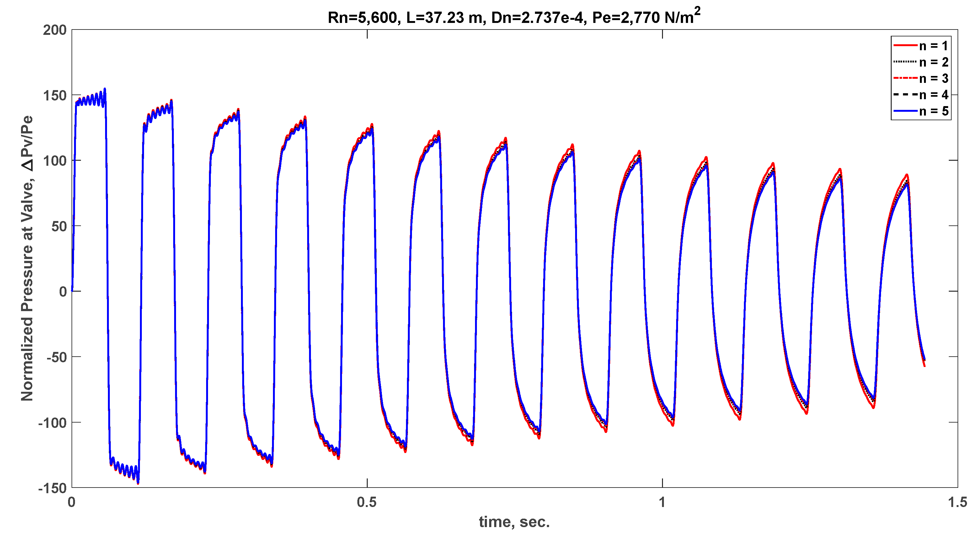
Figure 5.
Schematic of a line with a pump and valve.
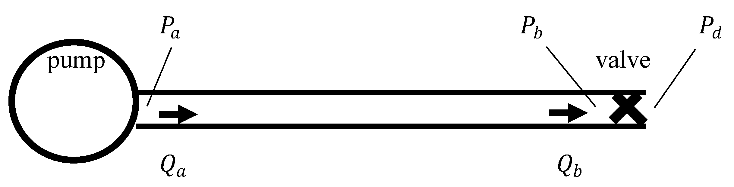
Figure 6.
Frequency response of the transfer function in Eq. (20) for q = 10.
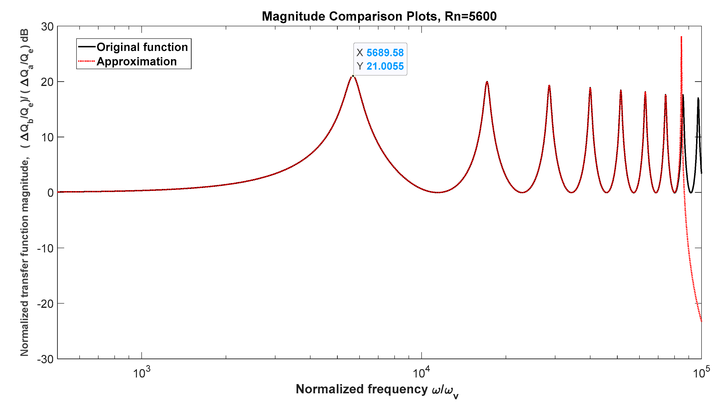
Figure 7.
Schematic of a rotary actuator speed control system.
Disclaimer/Publisher’s Note: The statements, opinions and data contained in all publications are solely those of the individual author(s) and contributor(s) and not of MDPI and/or the editor(s). MDPI and/or the editor(s) disclaim responsibility for any injury to people or property resulting from any ideas, methods, instructions or products referred to in the content. |
© 2025 by the author. Licensee MDPI, Basel, Switzerland. This article is an open access article distributed under the terms and conditions of the Creative Commons Attribution (CC BY) license (http://creativecommons.org/licenses/by/4.0/).
Copyright: This open access article is published under a Creative Commons CC BY 4.0 license, which permit the free download, distribution, and reuse, provided that the author and preprint are cited in any reuse.


