
Submitted:
26 August 2025
Posted:
27 August 2025
You are already at the latest version
Abstract
After heavy snowfall in the rural Uinta Basin, Utah, elevated surface ozone can occur when a persistent, reinforcing pool of cold air traps emissions from local oil and gas industry operations. Insolation permits photolysis and unhealthy buildup of surface ozone. Wintertime ozone is rare in the U.S. Intermountain West—more so a summertime issue in urban areas—and historically predicted poorly in numerical models. It follows a better understanding of prevailing snow patterns is important for constructing predictive models of ozone concentration. The Basin’s location leeward of the Wasatch Mountains provides conditions for a precipitation shadow, where rain or snow accumulation is suppressed by sinking air close to the lee. Mechanically, in westerly flow during winter, descending air parcels may accelerate, warm, and dry, hence clearing clouds that limit snowfall. Complicating spatial variations, wind-driven forcing may erode snow depth through drifting, melting, sublimation, etc. Sparse in situ observations and poor coverage of low-elevation radar tilts blocked by surrounding terrain compound the difficulty of snow-depth prediction, and due to tight connection with ozone formation, complicating prediction of snow sufficient to initiate the cold pool reinforcing feedback loop. Expectedly, ozone concentration observations track with snow coverage; more challenging was diagnosing a shadow effect and impact on ozone due to data sparsity and noise. The uncertainty but importance in linking snowfall variation to serious impacts of ozone levels on economy and public health motivates efforts to improve the region’s snow-depth measurements for purposes of nowcasting and machine-learning training.
Keywords:
ozone
; air quality
; mountain meteorology
; snow shadow
; precipitation shadow
1. Introduction
Episodes of elevated surface ozone concentrations may occur during winter in the Uinta Basin 1, eastern Utah, USA (Figure 1). These occur when snowfall persists under a temperature inversion for multiple days [1]; i.e., when cold air pools in the Basin, reversing the typical lapse of temperature with height. This inverted thermal setup traps volatile organics 2 and nitrogen oxides (NOx) emitted from nearby oil and gas industry [2,3]. Incoming solar radiation is sufficient to drive photolysis but too weak to melt snow sufficiently to counteract nocturnal katabatic winds that fill the Basin with cold, dense drainage flow from the surrounding high terrain [4]. High surface albedo maintains the feedback loop by reflecting insolation; critically, this actinic flux extends the path length for photolysis and increases ozone production, resulting in unhealthy air quality that can exceed national U.S. regulatory limits [5]. Despite the importance of snowfall to the Uinta Basin winter-ozone system—as seen in Figure 2 correlating local snow depth and ozone concentration—the influence of terrain on snowfall variation remains poorly understood in part due to difficulty in high-resolution modeling [6] or sparse data in rural areas. Understanding spatial variation in snow depth at the Basin floor is critical for creating improved prediction models or training statistical models [7,8].
Outside of wildfire-driven ozone episodes [9,10] and stratospheric intrusions [11], Uinta Basin ozone episodes are intermittent in their wintertime occurrence [7]. The phenomenon is rare, otherwise documented occasionally in, e.g., similar mountainous basins with oil and gas operations such as the Upper Green River Basin near Pinedale, Wyoming [12], and northern [13] and eastern China [14,15]. Ozone is more familiar as a summertime problem due to intense sunshine and more anthropogenic pollution sources in cities like Los Angeles [16], Beijing [17], Salt Lake City [18], etc. Elevated levels may also occur in rural areas with summertime oil and gas industrial emissions [19]. Health studies link elevated ozone levels with added respiratory stress, particularly for sensitive groups with conditions like asthma [20,21,22]. Regulatory responses in the USA are within purview of the Environmental Protection Agency (EPA) which set the National Ambient Air Quality Standards (NAAQS) threshold at 70 ppb for ozone. Predicting elevated levels of ozone is important for both public health and protecting the local economy from sanctions and economic ramifications. Multiple days of high ozone concentrations can trigger non-attainment designations and limits on industry operations. Hence, better understanding is in the interest of all stakeholders and the public [23], not only of scientific interest.
However, predicting air quality is a challenge in mountainous regions [24,25], in part due to complex interactions between atmospheric flow and orographic features [26][pp.327–334]. Subsequent mechanisms (mountain waves, adiabatic effects, etc.) perturb windward flow characteristics and dictate many features on the leeward microclimate [27]. One such phenomenon, the precipitation shadow effect, is seen as increasing rain- or snowfall as one moves further leeward of a mountain range [24] that are typically “more complex than the textbook explanation" [28]. It is defined by the American Meteorological Society as “...a region of sharply reduced precipitation on the lee side of an orographic barrier.“[29] The current study studies snowfall, but most documented cases involve variations in rainfall. Fundamentally, both phenomena occur through the same mechanism:
- Moist flow encounters higher terrain and is forced upward
- Rising air parcels cool, and resulting condensed water liquid precipitates predominately on the windward side
- This process depletes air parcels of moisture
- When drier air descends on the leeward side, it warms adiabatically, further drying air parcels.
- Hence, less moisture is available for precipitation, and the subsiding, dry air creates a “shadow" of reduced snowfall or rainfall.
Strong adiabatic warming (i.e., from compression under gravity) can cause a föhn effect [30] on the leeward side that can cause maximum dry-bulb temperatures that exceed those at locations typically warmer [31][e.g.,][]. This warming can lead to a notorious “snow-eater" wind seen in, e.g., the European Alps [24,32], where snow melts noticeably in the mountain-crest wake. Warming, drying winds can also exacerbate wildfire risks such as in destructive Santa Ana/Los Angeles events in the southwestern U.S. [33,34,35]. Further, the sensitivity of snow depth to snow-water equivalent and humidity (e.g., sublimation) are further uncertainties that gives the prediction of snow depth challenges not seen in rain shadows.
Regional studies, e.g., p.1 Mansfield [7] state as self-evident that a snow shadow exists in the Basin; however, the authors are not aware of formal documentation or quantification of a Uinta Basin snow shadow. The present study gauges evidence of this received wisdom, especially given the importance of snowfall for initiating the winter-ozone feedback loop. Observations of meteorological and air-quality parameters are critical for the Basin’s ozone warning program [8,23], both in nowcasting (i.e., real-time monitoring of observations) and forecast-model optimization (whether evaluation or machine-learning training). We restrict our focus to snowfall events with predominantly westerly flow at Wasatch crest height, due to its prevailing frequency and association with textbook snow-bearing storms [36]. We identify several important gaps that limit our understanding of spatial variation of snow depth in the Uinta Basin, and hence winter ozone formation:
- Do we find evidence of a Uinta Basin snow shadow? This would appear as less snow in the lee of the Wasatch than on the windward slopes, the challenge of a fair comparison in varying terrain notwithstanding;
- Do we see an impact of spatial snowfall variations on ozone levels? A greater extent of snow coverage would provide conditions associated with unhealthy build-up of ozone. If less snow falls in the western extent of the Basin, does this restrict ozone levels?;
- How certain are our data in rural, complex terrain? High uncertainty reduces the rigor of prediction, evaluation, and conceptual models. Data from in situ meteorological and chemistry sensors are sparse in comparison to urban regions, and Doppler radar data poorly samples the Basin. This is inherent noise.
We begin by reviewing pertinent studies that progressively link the meteorological impact of snow-depth variation on air chemistry and ozone formation.
2. Background
The rarity of elevated wintertime surface ozone stems from the need to balance multiple factors before winter ozone can be reliably generated:
- Equatorward enough to receive sufficient sunlight for photolysis
- Poleward enough to preserve snow (less insolation and lower temperatures)
- The higher the elevation, the stronger the insolation
- Complex terrain cold-pool formation in mountain valleys and basins
- Precursors to ozone (i.e., volatile organics; NOx)
Ozone episodes are most frequent in the second half of winter [7], whose higher solar angles in February balance thermal disruption to persistent cold pools. Precursor emissions, assumed constant for the purposes of this discussion, are provided mostly by oil and gas industry operations. The high elevation also means background levels—even without human influence—are higher due to natural seepage and stratospheric intrusion of ozone-rich air. Snow-bearing weather systems generally move with a west-to-east component, though sensitivity of snowfall to wind direction in Utah [37] is outside the scope of the current study.
We consider two windstorm subtypes. So-called Wasatch windstorms [38,39] occur in easterly flow north of the Uinta Mountains (Figure 1). Flow blocked by the west–east Uinta Mountains is funneled towards lower surface pressure in Salt Lake City. When easterlies cross the Wasatch Range, windstorms can occur in Davis County (Figure 1), gusts measured as exceeding 46 (102 mph; 89 kt). Air does not warm: the descending wind is similar to a waterfall [38]: a pooling of cold air behind (east of) the crest that spills over the crest (Figure 1).
Conversely, further south, westerly flow crossing the Wasatch into the Uinta Basin has a steeper rise-and-fall for moist airflow to navigate. During (north-)westerlies, air is forced to rise from ~1300 m (4250 ft) to ~3500 m at Wasatch crest-level (this results in the self-described “Greatest Snow On Earth" [40]). Drier air parcels then descend into the Heber Valley (~1700 m), or continue over terrain exceeding 3000 m (9800 ft) between Heber City and Duchesne (~1700 m) (cf. terrain in Figure 1 and Figure 3). Thus, understanding flow in complex: will the flow descend into the Heber Valley (this may depend on atmospheric stability)? Now in our area of interest, flow descends to the Basin’s lowest point ~1400 m (4600 ft) near Ouray (Figure 1) and ascends gradually to a ~2500 m plateau east of the Utah–Colorado border. Completing the bowl-like terrain pattern, the pre-Cambrian Uinta Range bound the Basin to the north at 3500–4000 m; the Book and Roan Cliffs (generally, the Tavaputs Plateau) likewise at ~3000 m to the south.
Stockham et al. [27] found a standard definition of rain shadows can lack important local distinctions, e.g., Peak District, UK. Representative timescales and physical mechanisms vary with latitude, season, etc. Rain shadows occurred much less frequently than hypothesized: fewer than 1 in 5 days with prevailing wind conditions. Representative of numerical prediction as a whole, Ghan et al. [41] found climate models may struggle to capture precipitation shadows, consistently showing “too little precipitation on the windward side" and vice versa: their models could not reproduce “sub-grid rain shadows"; i.e., a suppression of precipitation occurring at scales below that which the model can capture (i.e., the scale of truncation).
Even in the absence of complex topography, snow accumulation can be highly spatially variable. Snow depth is sensitive to numerous mechanisms and surface characteristics, including sublimation, melting, refreezing, settling, vegetation type, soil temperature, and the lofting and drifting of snow. The reported depth of snow is modulated by wind-driven sublimation [42][p. 189], potentially relevant given the long fetch along the Basin’s longest axis. Modeling evaporation and sublimation from a Basin snow coverage can lead to unrealistic snow depth values [43][p. 2423], adding to uncertainty from surface roughness (friction). Further, drifting and settling in varying terrain degrades representivity of snow reports. Estimation of melt is reliable [44], but errors in soil temperature and intermittent melt–freeze sequences can accumulate and not capture marginal freezing cases [45], degrade snow-water equivalent estimates [46], etc. Compacting snow makes the pack denser but shallower [47].
It is unknown to what magnitude these variations impact ozone concentration. Yet despite the challenges identified in conducting robust studies, snow shadows were documented in Maine, USA in 1942 [48], and in modest terrain in the USA northeast [49]. In Japan Kusaka et al. [50] documented an unorthodox snow shadow on the Sea of Japan coast, displaying parallels with US mountain phenomena [51] including involving seas or lakes [52] bearing similarities to the nearby Salt Lake City lake breezes [53].
3. Data and Methods
We recapitulate our main aim of exploring our observation dataset to determine whether there is the signature of a snow shadow mechanism, as defined above.
3.1. Study Area
Figure 1 shows broad regions used herein, chosen during initial work and for reference to areas in text. Stations that are listed as active in the Synoptic Weather data repository are plotted in Figure 4 with their station ID to highlight the contrast in the amount of snow-depth observations between the Wasatch Front and Uinta Basin (cf. terrain in Figure 1). Stations prefixed with “COOP" are volunteer-run National Oceans and Atmospheric Administration (NOAA) Cooperative Stations (https://www.weather.gov/coop/overview, accessed 1 June 2025) that report snow-depth manually once-daily with precision to the nearest 1 in (2.5 cm). This coarse sampling in time, space, and precision poses an obstacle to finer, robust snow-depth measurement, especially in the western part of the Basin leeward of the highest terrain (near Duchesne in Figure 1 and Figure 4).
3.2. Cases and Data
Observation data is less reliable in complex terrain than flatter landscapes due to the low representivity of stations and poor spatial/temporal sampling. Further, observational noise is not consistent between stations: at least one station operated by the Bingham Research Center was manually corrected for animal interference, for example, while we identified another site prone to drifting near the sensor. Preliminary work revealed periods of unreliable data: measurement gaps, obviously spurious outliers, and limited spatial coverage to increase confidence of observation fidelity. We acquired NOAA GOES-satellite visible-channel imagery from the repository at https://www.star.nesdis.noaa.gov/goes/index.php to complement in situ observations for a basic yes/no for snow coverage in the study areas (Figure 1).
3.3. Data Collection
Utility of satellite is restricted by its infrequent sampling of the Basin (once or twice daily) and frequent cloud cover during times where information on snowfall is most useful. Further, there are few intersections of the relatively low frequency of satellite passes () and winter storm systems that bear snow for the Basin () required to trigger the feedback loop for ozone production (Figure 3).
Other satellite data relevant to the present topic [54,55], such as albedo or low-level lapse rates, are outside the current scope but have found limited success in preliminary work due to large uncertainty.
Doppler Radar
The Basin’s distance from the closest Doppler radars—part of the U.S. national radar network (NEXRAD)—limits detection of Basin precipitation due to terrain beam-blocking. Radar sites at Grand Junction (KGJX) and Salt Lake City/Promontory Point (KMTX) [56][][their Figure 1] can overshoot falling precipitation: as the beam radiates from the radome in a conical manner, a beam must be high enough to clear the Basin’s circumferential terrain but low enough to sample below cloud base. Resultant estimates of precipitation amounts are less reliable than, for instance, the downstream Great Plains region [57][][p. 2035]. In summer, cloud bases in the high desert can reach ~4 km AGL, meaning rain or hail may be detected on radar, but evaporation and/or sublimation of the precipitation shaft (i.e., virga) would occur undetected below the lowest possible beam (i.e., 0.2°). This would result in an overestimation of rainfall. Conversely, shallow Basin winter cold pools are O(100 m) [1,25]. This would result in underestimation of snowfall due to overshooting of the lowest radar beam. Due to the importance of radar coverage for predicting conditions for ozone formation, we inspect the sampling regions more closely by computing the lowest height of a radar beam above the Basin from the two radars in proximity (Figure 5). Beams blocked by terrain are masked with a black pixel and colored pixels show the minimum height above ground level. The figure reveals how poorly that precipitation might be sampled, particularly in the west and central Basin. (The mathematics of our computation is presented in Appendix A). The same problem of overshooting radar beams is documented elsewhere, including the windward Wasatch slopes as sampled from KMTX [36][their Figure 2]
To summarize: regions where this surface significantly exceeds Basin-floor elevations indicate poor radar sampling of precipitation due to blocking by the surrounding high terrain and inherent curvature upwards of the conical beam. Eastern parts of the Basin (near Vernal) are mostly sampled due to their line of sight to KGJX rather than KMTX blocked by the taller Wasatch Range. This creates high uncertainty for live viewers of radar data regarding precipitation reaching the surface (hence, so too the hydrometeor type). We see the signature of a so-called "radar hole" in later precipitation radar-derived estimates.
In Situ Meteorological Sensors
We obtain 20 years of archived data from Synoptic Weather repositories (https://synopticdata.com/national-mesonet-program/, accessed 1 January 2025), part of the U.S. National Mesonet Program. All sites reporting snow depth in our period of record and zones of interest are shown in Figure 4. The Bingham Research Center further deploys its own stations (those marked in red on Figure 4 maps) as part of its air quality network (UBAIR). Raw data is sent from the field site via cellular internet to Synoptic Weather repository archives almost immediately; however, multiple sources of error (e.g., drifting; animal interference; thermal contraction) necessitates careful postprocessing. Further automating this error correction method is an ongoing effort to improve availability of snow data for purposes of ozone forecasting.
Ozone concentrations were not necessarily sampled at the same site as snow depth but site choice heavily accounted for suitable coherence between both observations’ insight into the real state. The generalization of measured ozone concentration is uncertain and likely flow-dependent due to non-constant emission inventories across the Basin (e.g., oil and gas rigs opening in new locations, while old sites close). The changes are slow enough to enable skillful training of AI-based ozone predictions [8], but it remains difficult to anticipate step changes in industry operations, and hence ozone precursors.
Numerical Weather Prediction and RTMA Data
The national Air Quality Model (AQM), part of the next generation of NOAA NWP systems (the Unified Prediction System; [58]), runs at 13-km horizontal grid-spacing; as such, it can miss high-ozone events in basins such as the subject of this study due to small scales of mountain cold pools [59,60]. For instance, a high ozone event on Jan 31 2025 was not captured by AQM forecasts (Figure 6), while high ozone associated with wildfires in the U.S. Southwest were larger scale and within the purview of AQM simulation (Figure 6). This inability of traditional NWP models to adequately capture small-scale uncertainty drives exploration of alternative prediction techniques, such as statistical prediction of ozone that relies on good input data for training and pattern recognition. Output from experimental models [8] currently supports the Bingham Research Center’s yearly Ozone Alert program, where stakeholders receive periodic email about potential elevated-ozone episodes. In this context, use of a coarse model such as AQM is immediately discarded as mathematically incapable of resolving cold pools (and hence ozone concentrations; [61]) accurately in the Uinta Basin. Herein, we also deploy analyses from the High-Resolution Rapid Refresh (HRRR) model as a proxy for gridded “truth", i.e., forecast hour 0. We primarily inspect two analysis products to supplement observations of snow: its depth and spatial coverage.
It is understandably difficult to estimate precipitation amounts in complex terrain due to low representivity of stations, large variability in conditions, and sparsity of observations in remote areas. To supplement raw in situ observations, the Real-Time Mesoscale Analysis (RTMA) system was developed by the National Centers for Environmental Prediction (NCEP) to create more continuous maps of, e.g., precipitation across the USA at 5-km horizontal grid-spacing [62]. The system uses two-dimensional variational data assimilation (2DVAR), where the Jacobian (linearized observation operator) adjusts a prior model state towards an optimal combination of weather observations and model analyses, representing a best guess. Originally, RTMA ingested Rapid Update Cycle model forecasts down-scaled from 13-km to 5-km horizontal grid-spacing as background fields; later, the system incorporated HRRR backgrounds that improved analysis quality further [63].
Given our interest in air quality correlated with mountain meteorology, we note methods in RTMA that include terrain-following techniques designed to account for complex orography, e.g., anisotropic background error covariances that follow terrain gradients [62]. However, limitations remain outside of flat terrain [63] such as in Utah within the U.S. Intermountain West [62][their Figure 8]: some RTMA products displayed no skill in the West over raw observations. These shortcomings were acknowledged, including issues with quality control and optimization for cases in small-scale valleys and basins. Tyndall and Horel [64] found disproportionate impacts from mountainous stations and rail-network sensors in remote locations such as central–east Utah, including the Uinta Basin. Accordingly, more advanced systems are required to capture high-complexity flow using, e.g., flow-dependent covariance matrices [65], though even advanced methods performed poorly in sloping terrain and elevations above ~1 km—typical of Utah’s ranges and basins [66].
For quantitative precipitation estimates (QPE), RTMA ingests Doppler radar data from the NEXRAD WSR-88D national network operated by the National Weather Service. De Pondeca et al. [62] explain how radar data are combined with rain gauge information as Stage II analyses further compared and detailed in [67][][and refs. therein]. However, in regions such as the Uinta Basin with poor radar coverage (Figure 5) and sparse in situ observations (Figure 4), the existing high-terrain issue of poor representivity and unreliable optimization schemes is compounded further. Accordingly, we maintain a focus on trustworthiness of RTMA data in the Basin.
3.4. Filtering and Post-Processing
A sparse network of snowfall observations hinders our study of the snow and ozone geographic variation, creating challenges for understanding the underlying processes and developing predictive tools. Despite quality control of data before it is retrieved, prekliminary work showed need to apply further post-processing. Errors were inconsistent, likely due to numerous causes of spurious reports. Before developing a filtering method, we subjectively identified outliers in snow depth measurements from weather stations across the Uinta Basin, Utah. Errors were typically spikes diverging from a recognizable quasi-linear time series. From the team’s own work in field installations and maintenance of stations, we found errors that resulted from sensor malfunctions, transmission noise, or difficult and changing environmental conditions.
We must choose a filter that is balanced: extremes must be handled carefully to avoid squashing events important to our air-quality context. Further, and with unavoidable subjectivity, the processing should not fabricate large windows in time from which we infer results. In preliminary testing, we found the Hampel filter [68][][and refs. therein] most effective when evaluated subjectively by eye. It was less likely to smooth out extreme values in preliminary testing than other filters, and was robust when the chosen window was small enough to preserve persistent snowfall. The filter operates by sub-setting a sliding window of size , computing median-absolute-deviation (MAD) to identify outliers, and replacing them with a subset median if they exceed a multiple n of the MAD. The drawback of the Hampel filter is degraded performance in symmetric Gaussian-noise regimes. Ultimately, its best subjective performance justified use of the Hampel method to filter snowfall time series used herein. We do not filter the COOP network (i.e., once-daily quantized at 2.54 cm intervals). The group will deploy the above filtering method on time series shown on the Research Center’s experimental Basin air-quality portal at www.basinwx.com.
4. Results
Reiterating our goals, we review multiple sources of data—observations, RTMA, reanalyses—to quantify any association between snow depth and distance from the Wasatch, and whether elevated ozone patterns correspond to those in snow coverage. For reader reference, the study area begins winter in UTC-7 and moves to UTC-6 by its conclusion.
Case 1: Late February 2023
In the first half of this case, elevated ozone occurred in the Basin (Figure 7). Snow depth during this time was sufficient in the Basin (Figure 8) to allow buildup of ozone.
The early snow was captured in the HRRR analyses broadly correctly (not shown) with a general underestimate of snow depth and covering, potentially related to lack of radar detection, sampling by satellite, weather observation station data, etc. Nonetheless, there is suggestion of less snowfall (a snow shadow) in observed data for the snow passage round 23 February (contrast the two site groups in Figure 8). Relating this to the larger context, we see that a snow shadow, should it exist, is not reducing snowfall coverage to an amount that precludes ozone buildup. Perhaps it reduces the probability a cold pool will form, all else assumed constant; further exploration is outside the scope of the current study.
We derived an estimate of total storm accumulation (or liquid equivalent, if snow) adding 6 days’ totals per grid point in RTMA data. Evidently, the estimated accumulated precipitation product from RTMA (Figure 9) did not detect snowfall during the week with a critical snow-pack: moreover, the radar “hole" is evident in near-zero accumulations for the Basin despite observed snowfall (implied by satellite imagery in Figure 11). The precipitation product in Figure 9 and at other times (not shown) often display a brighter band emanating from the radar location, marking a region (e.g., crest level) where beams pass unobstructed until reaching the hydrometeor of interest.
The gross underestimate of snowfall in the Basin likely stems from under-sampling when terrain blocks Doppler radar (cf. Figure 5) and not remedied by incorporation of sparse rain-gauge data when producing the Stage II gridded QPE product. Indeed, the RTMA product’s use of radar data is conspicuous by its prominent striping.
Figure 10.
HRRR analyses of snow coverage, initialized and valid at 1200 UTC, 24 February 2023.
Analysis of the February 2023 episode reveals mixed evidence for snow shadow effects. While satellite imagery (Figure 11) shows widespread snow coverage across the Basin, RTMA precipitation estimates (Figure 9) failed to detect snowfall in the western Basin during the 22–28 February period, likely due to radar beam blocking rather than actual precipitation differences. This creates an artifact that presents similarly (but erroneously) as a snow shadow. Ozone concentrations (Figure 7) reached 70–100 ppb in Basin locations while remaining around 40 ppb on the Wasatch Front, consistent with the winter ozone formation mechanism requiring persistent snow cover and trapped precursors. The episode demonstrates that even modest snow accumulations can sustain ozone episodes when combined with stable atmospheric conditions shown in Figure 3. Contributions to ozone concentration from factors additional to spatial variation of snow depth (e.g., elevation; proximity to industry operations) may be inextricable and preclude more certain diagnoses.
Figure 11.
Visible satellite image (MODIS Terra), valid 2203 UTC, 24 February 2023, showing snow throughout the Uinta Basin.
Figure 11.
Visible satellite image (MODIS Terra), valid 2203 UTC, 24 February 2023, showing snow throughout the Uinta Basin.
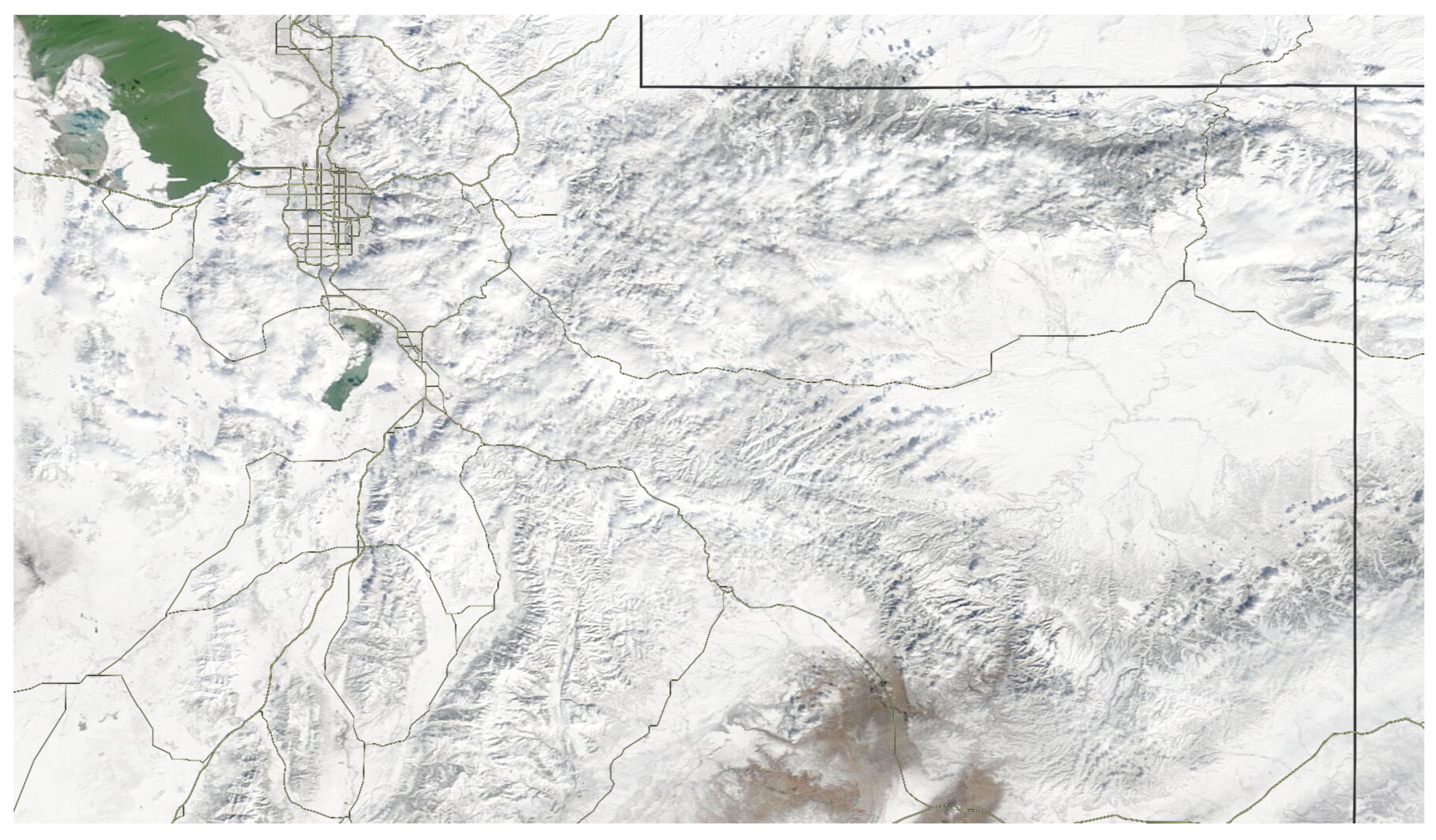
Figure 12.
HRRR analyses of 2-m temperature and dewpoint initialized at 1200 UTC, 24 February , and average over the six days to capture broad patterns (larger smoothing in line with high uncertainty) in the period 0000 UTC 27 January 2025 to 0000 UTC 28 January 2025. Simulated snow cover is shown in Figure 14 during this period.
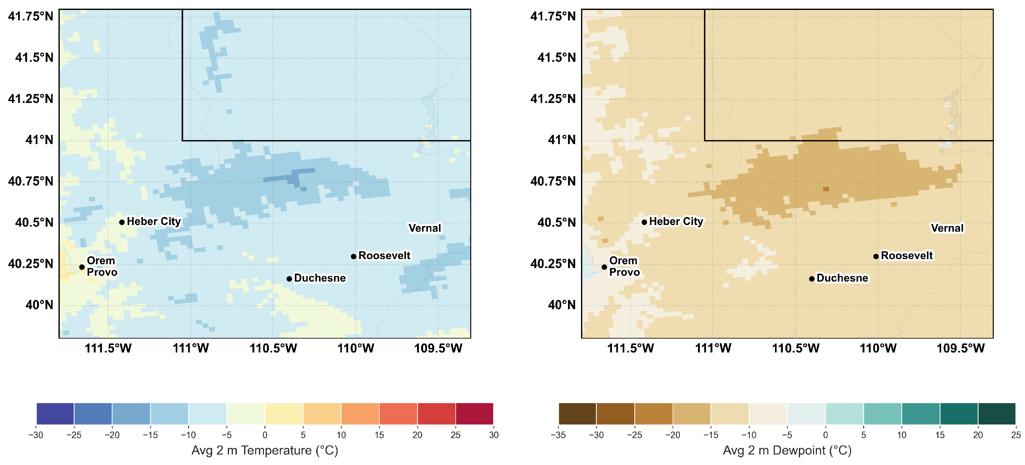
In Figure 13, we note Roosevelt’s position in line with stronger flow channeled through mountain canyons, which may indicate increased melt (note the snowfall and melt around 0900 UTC, 27 January 2025, in Figure 13). Unfortunately, ozone concentration data was missing on this day and precludes comparison with other stations in the region in Figure 12 — further highlighting our frustration with data gaps and sparsity.
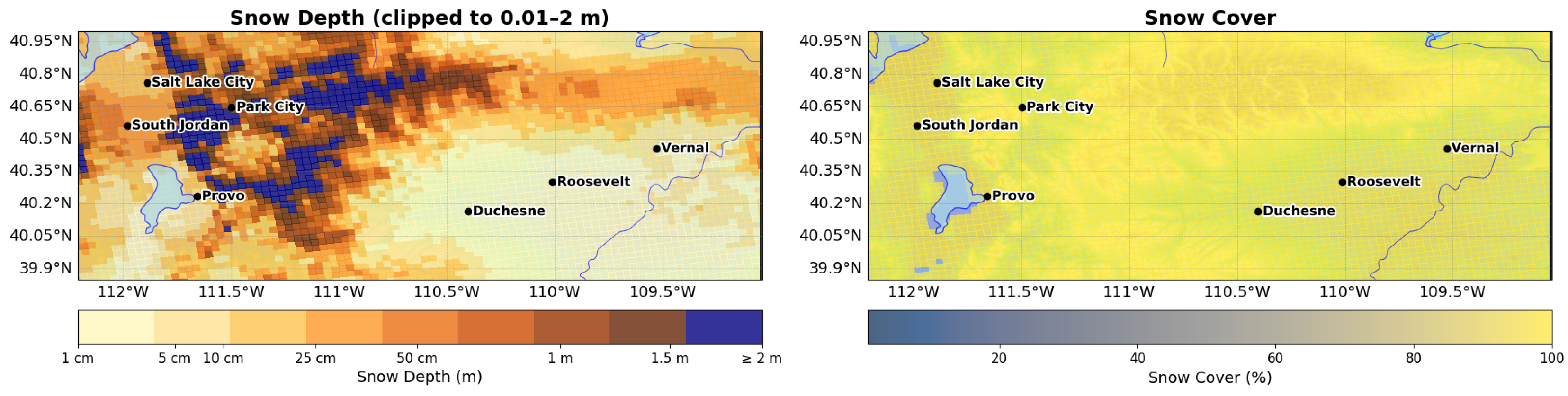
The January 2025 case provides better RTMA–observation agreement, with HRRR analyses (Figure 14) capturing both snow depth and coverage patterns visible in satellite imagery (Figure 15).
Figure 14.
An analysis of snow depth and coverage at 0000 UTC on 27 January 2025.
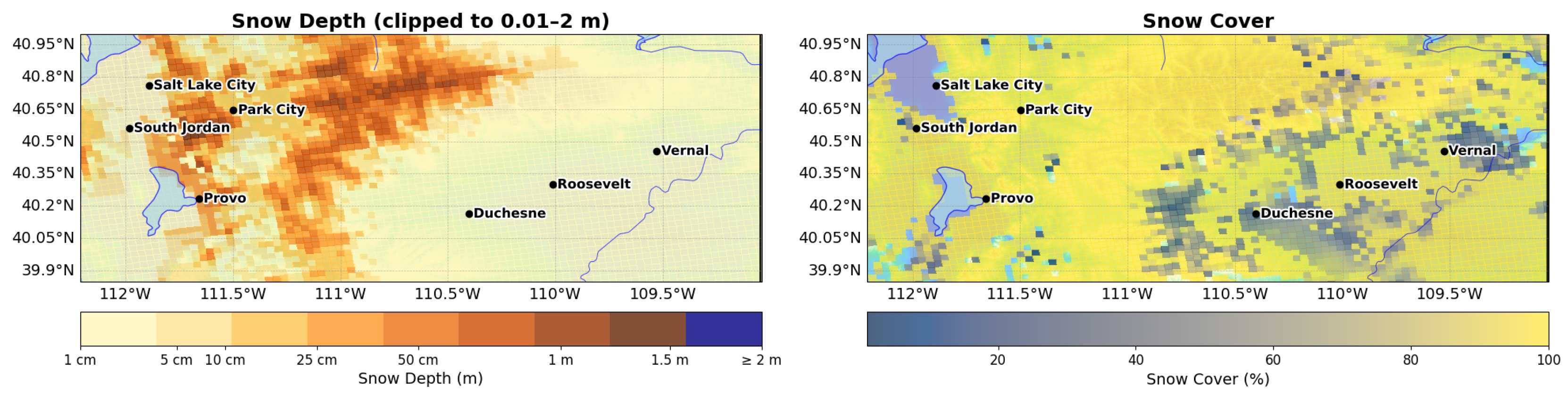
Figure 15.
Visible satellite image (MODIS Terra), valid 2203 UTC, 27 January 2025, showing snow coverage across the study region.
Figure 15.
Visible satellite image (MODIS Terra), valid 2203 UTC, 27 January 2025, showing snow coverage across the study region.
Figure 16.
Total storm precipitation (snow-water equivalent if frozen) from the RTMA gridded observation product valid roughly at the end of the second case-study period.)
Figure 16.
Total storm precipitation (snow-water equivalent if frozen) from the RTMA gridded observation product valid roughly at the end of the second case-study period.)
Snow depths in both analyses and observations show gradual increase from west to east across the Basin floor (Figure 13, potentially indicating shadow effects, though corroboration with sparse observations is difficult. Basin ozone concentrations touched the 70 ppb threshold during this episode (not shown), with peak values correlating spatially with areas of persistent snow cover identified in both model analyses and satellite data. These are supporting signs of a connection between spatial heterogeneity and ozone concentration, but do not explicitly suggest the presence of a snow shadow.
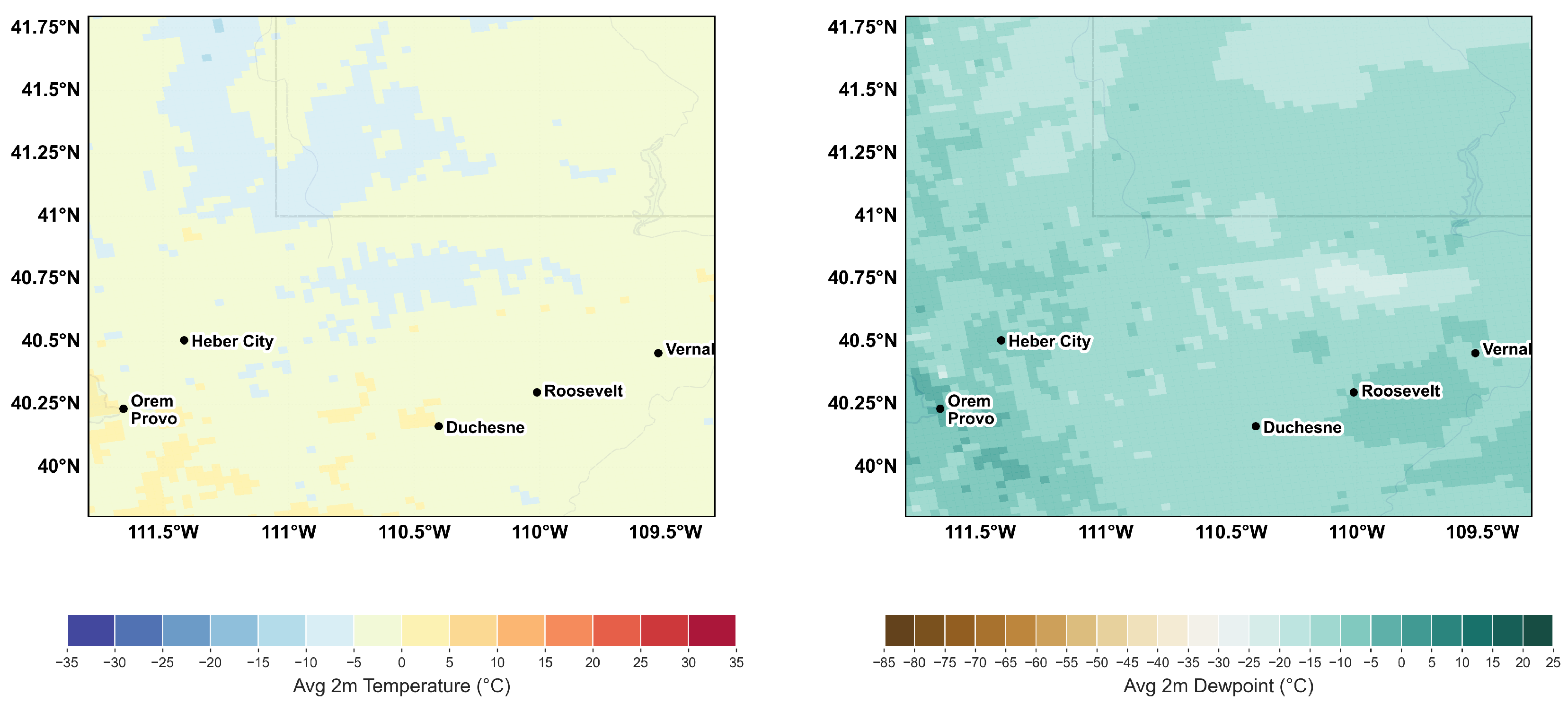
Surface dry-bulb and dew-point temperatures (Figure 17) display a wider-scale drying that more holistically explains a reduction in precipitation Basin-wide, albeit not in the lee of the higher terrain. Albeit a weak signal in HRRR analyses, dewpoints increase and drybulb (“sensible") temperatures decrease slightly as one moves east from the Wasatch: compare Roosevelt to Duchesne in Figure 17a,b. Conceptually, weather effectively passes over the Basin—especially so during stable winter episodes that reinforce over a snow pack—and this may track with a lack of documented windstorms or damage in the lee of surrounding terrain.
Our analysis faced significant challenges in documenting snow shadow effects and air quality implications. While qualitative evidence supported some elements of our initial science questions, quantitative confirmation is hindered by: (1) radar beam blocking that creates artificial precipitation holes in gridded products; (2) sparse in situ observations that inadequately sample spatial gradients; and (3) complex terrain that confounds windward–leeward comparisons. Despite observational limitations, connections emerge between snow coverage and ozone formation. As in many other cases documented in Bingham Research Center et al. [23] and similar annual reports before it, episodes with widespread Basin snow coverage produce elevated ozone concentrations exceeding 70 ppb when other conditions allow (stable, high pressure; sufficient insolation), while periods with patchy or absent snow typically show near-background ozone levels regardless of precursor emissions. This reminds operational forecasters of the critical role in albedo for maintaining ozone-producing boundary layers (Figure 3).
5. Conclusions
We set out to address three key questions regarding snow shadows and winter ozone formation in the Uinta Basin:
Do we find evidence of a Uinta Basin snow shadow? Broadly, yes. While the mathematical theory and historical observations suggest reduced precipitation leeward of the Wasatch Mountains, data-quality limitations prevent definitive confirmation. RTMA precipitation estimates are unreliable due to radar coverage gaps, and while it appears to show a clear snow-shadow pattern in our case studies (and other preliminary work), this is likely an artifact of sparse near-surface radar data. Surface observations are too sparse for robust spatial analysis. However, satellite corroborated HRRR numerical estimates of snow coverage; fair comparison of different elevations remains an open question.
Do we see an impact of spatial snowfall variations on ozone levels? Yes: in the first case (e.g., Figure 7), Basin stations sampled high ozone daily maxima (i.e., over 70 ppb) absent along the Wasatch Front (windward); regional connections may exist between snow coverage extent and ozone concentrations, but elevation (cold pool strength) and contributions to high ozone from proximity to industry are also inextricable factors. Fine-scale impacts of precipitation gradients on ozone spatial patterns remain difficult to quantify, partly due to a small sample size.
How certain are our data in rural, complex terrain? Uncertainty is substantial and limits predictive and diagnostic capability. Radar beam blocking creates systematic gaps in precipitation monitoring; sparse surface networks inadequately capture spatial gradients; uncertainty hampers the accuracy of our alert communications for industry regulatory compliance and public health.
There are unique challenges of predicting elevated winter ozone in the Uinta Basin, Utah, USA. Primarily, the dependence of ozone formation on sufficient snow depth necessitates good knowledge of the current state for both nowcasting and initiating numerical prediction of high-ozone episodes. In the authors’ experience, it is received wisdom in the local community that the Basin lies in a snow shadow: a region with lower snowfall accumulations close to the lee of the crest compared to surrounding areas not subject to these theorized descending lee winds. The lower humidity and snowfall is evident in our visualizations, corroborating an accepted truth. However, during the course of performing a more rigorous snow-shadow diagnosis, and subsequent impact on ozone formation and prediction, we were impeded by relatively low data quality (sparsity; representivity; sampling frequency or consistency) that hampered more robust assessments of precipitation estimates. Further factors included copious radar-beam blocking, a sparse observation network, and infrequent satellite passes.
Some adjacent takeaway points include:
- Poor estimates of precipitation accumulation from RTMA is insufficiently corrected by a sparse network of radar and in situ observations;
- In summer, cloud base may extend to 4 km AGL; hence beams can sample precipitation that may evaporate or sublimate between this level and the surface (virga), which results in overestimation from radar returns;
- In winter, cloud bases are within the lowest kilometer, meaning any precipitation is unlikely to be sampled despite lower likelihood of virga from the shorter, colder path to the surface.
While it is less important to label a phenomenon with as many caveats as outlined above, understanding sources of observation and model error is paramount to improve training of machine-learning or artificial-intelligence models.
High uncertainty should motivate larger, coarser ensembles (of traditional or AI sorted alike), rather than running at finer resolutions. In balance, vertical grid spacing must be fine enough to capture a shallow cold pool in a traditional NWP model. It is the curse of dimensionality, however, that prevents the evaluator from knowing if the complexity is precision rather than accuracy.
5.1. Future Work
Research avenues slated for ongoing and future investigation include:
- Data analysis over a longer time period;
- Low-cost snow-depth sensors [69][e.g.,][] that reporting live onto national networks;
- Analysis of ozone concentration and snowfall amounts for weather systems with different prevailing wind directions;
- Identification of new observation sites that would most benefit ozone and snow prediction [70][e.g.,][];
- Methods to extract information (despite trends in industry operations and snowfall intermittency) with further statistical processing [71].
Artificial Intelligence statement
The authors used the following large-language models during the course of the research, but no generated text output was used verbatim in the manuscript, and all output was fact-checked by the authors. For lower-complexity use-cases, we used DeepSeek R1 1776, an uncensored instance of the open-sourced DeepSeek package hosted by Perplexity in the United States. On top of good performance, a motivation for use of DeepSeek R1 1776 over, e.g., traditional web searches was its lower energy footprint based on author estimates.
| OpenAI GPT o4-mini-high | Python coding assistance |
| OpenAI GPT o3 | Research brainstorming |
| OpenAI Codex | LaTeX typesetting fixes |
| Claude Opus 4.x | Python visualization assistance |
| DeepSeek R1 1776 | Information collation |
Author Contributions
Conceptualization, MJD and JRL; methodology, MJD, JRL, SNL, and TN; software, MJD, JRL, SNL, TN, TDC, and KZ; validation, MJD and JRL; formal analysis, MJD and JRL; fitting metrics, JRL; investigation, MJD, JRL, SNL, TN, TDC, and KZ; resources, SNL; data curation, MJD, JRL, SNL, TN, TDC, and KZ; writing—original draft preparation, MJD and JRL; writing—review and editing, MJD, JRL, SNL, TN, TDC, and KZ; visualization, MJD and JRL; supervision, SNL and JRL; project administration, JRL; funding acquisition, SNL. All authors have read and agreed to the published version of the manuscript.
Funding
This work was funded by Uintah County Special Service District 1 and the Utah Legislature
Data Availability Statement
Code used herein is available in repositories hosted at www.github.com/bingham-research-center, comprising python functions and worked Jupyter notebooks. Much of this development is and was assisted by generative AI output from GitHub Copilot A.I. and other large-language models listed above. Operational products improved by the current work are hosted at www.basinwx.com, operated on an experimental basis by the Bingham Research Center.
Acknowledgments
The authors thank Alex Jacques at Synoptic Weather and John Horel at the University of Utah for work in sending our group’s observations to the Synoptic Weather repository; non-credited co-authors at the Bingham Research Center for their assistance with apparatus and data collection; Brian Blaylock for continued maintenance of key python packages SynopticPy and Herbie; Pamela Gardner for reviewing an earlier draft of the manuscript; local insight and initial conversation with Tracie Kingsford; anonymous reviewers and journal staff during the submission process for their help in quality and processing.
Conflicts of Interest
The authors declare no conflicts of interest.
Abbreviations
Some key abbreviations used in this manuscript:
| NOx | Nitrogen oxides |
| VOCs | Volatile organic compounds |
| BRC | Bingham Research center |
| USU | Utah State University |
| NEXRAD | Next Generation Radar |
| KMTX | Promentary Point (Salt Lake City) NEXRAD site |
| KGTX | Grand Junction NEXRAD site |
| KVEL | Vernal Regional Airport |
| KSLC | Salt Lake International Airport |
| EPA | Environmental Protection Agency |
| NAAQS | National Ambient Air Quality Standards |
| NOAA | National Oceans and Atmospheric Agency |
| UFS | Unified Forecasting System |
| RTMA | Real-Time Mesoscale Analysis |
| HRRR | High Resolution Rapid Refresh (model) |
| AQM | Air Quality Model (NOAA UFS) |
| AGL | Above Ground Level |
Appendix A.
Computation of radar-beam height and terrain blocking We first obtained high-resolution Digital Elevation Model (DEM) data covering the Uinta Basin. We use the USGS ~10 m grid downsampled to a grid with spacing of 1°-by-1° in line with computational limitations. The DEM ranges over a bounding box extending from the Salt Lake City (KMTX) and Grand Junction (KGJX) radars (top left and bottom right, respectively, in the six Figure 5 panels.
Appendix Grid Definition
We define a regular grid of longitude–latitude points
with spacings chosen so that the horizontal cell-size does not exceed the vertical resolution requirements of the beam-width footprint at maximum range [72].
For each grid point and for each radar site we compute the slant range using the spherical-Earth approximation:
where m is the assumed mean Earth radius.
Appendix Beam Height Computation
At each slant range we compute the beam height above mean sea level for the lowest elevation tilt (0.2° for KMTX and KGJX in low-level elevation mode):
where is the radar site elevation. The first term accounts for the site height, the second for the linear beam rise, and the third for Earth’s curvature (rationale taken from National Weather Service recommendations for correcting beam-bending correction at https://www.weather.gov/media/lsx/wcm/decision/RadarTraining2010.pdf, accessed 1 May 2025.)
Let denote the terrain elevation from the DEM at grid cell . We define clearance
A grid cell is not masked (visible) if , and blocked otherwise. For each cell we can record the minimum sampling height
and optionally take the point-wise minimum over both radars:
but results from this computation were used in analysis and not shown herein.
References
- Neemann, E.M.; Crosman, E.T.; Horel, J.D.; Avey, L. Simulations of a cold-air pool associated with elevated wintertime ozone in the Uintah Basin, Utah. Atmos. Chem. Phys. 2015, 15, 135–151. [Google Scholar] [CrossRef]
- Lyman, S.; Tran, T. Inversion structure and winter ozone distribution in the Uintah Basin, Utah, U.S.A. Atmos. Environ. 2015, 123, 156–165. [Google Scholar] [CrossRef]
- Schnell, R.C.; Oltmans, S.J.; Neely, R.R.; Endres, M.S.; Molenar, J.V.; White, A.B. Rapid photochemical production of ozone at high concentrations in a rural site during winter. Nat. Geosci. 2009, 2, 120–122. [Google Scholar] [CrossRef]
- Schnell, R.C.; Johnson, B.J.; Oltmans, S.J.; Cullis, P.; Sterling, C.; Hall, E.; Jordan, A.; Helmig, D.; Petron, G.; Ahmadov, R.; et al. Quantifying wintertime boundary layer ozone production from frequent profile measurements in the Uinta Basin, UT, oil and gas region. J. Geophys. Res. 2016, 121. [Google Scholar] [CrossRef]
- Edwards, P.M.; Brown, S.S.; Roberts, J.M.; Ahmadov, R.; Banta, R.M.; deGouw, J.A.; Dubé, W.P.; Field, R.A.; Flynn, J.H.; Gilman, J.B.; et al. High winter ozone pollution from carbonyl photolysis in an oil and gas basin. Nature 2014, 514, 351–354. [Google Scholar] [CrossRef]
- Jones, C.; Tran, H.; Tran, T.; Lyman, S. Assimilating satellite-derived snow cover and albedo data to improve 3-D weather and photochemical models. Atmosphere (Basel) 2024, 15, 954. [Google Scholar] [CrossRef]
- Mansfield, M.L. Statistical analysis of winter ozone exceedances in the Uintah Basin, Utah, USA. J. Air Waste Manag. Assoc. 2018, 68, 403–414. [Google Scholar] [CrossRef]
- Lawson, J.R.; Lyman, S.N. A preliminary fuzzy inference system for predicting atmospheric ozone in an intermountain basin. Air 2024, 2, 337–361. [Google Scholar] [CrossRef]
- Xu, L.; Crounse, J.D.; Vasquez, K.T.; Allen, H.; Wennberg, P.O.; Bourgeois, I.; Brown, S.S.; Campuzano-Jost, P.; Coggon, M.M.; Crawford, J.H.; Ozone chemistry in western, U.S.; et al. wildfire plumes. Sci. Adv. 2021, 7, eabl3648. [Google Scholar] [CrossRef] [PubMed]
- Jaffe, D.A.; Wigder, N.L. Ozone production from wildfires: A critical review. Atmos. Environ. (1994) 2012, 51, 1–10. [Google Scholar] [CrossRef]
- Lin, M.; Fiore, A.M.; Cooper, O.R.; Horowitz, L.W.; Langford, A.O.; Levy, H.; Johnson, B.J.; Naik, V.; Oltmans, S.J.; Senff, C.J. Springtime high surface ozone events over the western United States: Quantifying the role of stratospheric intrusions. Journal of Geophysical Research: Atmospheres 2012, 117. [Google Scholar] [CrossRef]
- Mansfield, M.L.; Hall, C.F. A survey of valleys and basins of the western United States for the capacity to produce winter ozone. J. Air Waste Manag. Assoc. 2018, 68, 909–919. [Google Scholar] [CrossRef] [PubMed]
- Tang, G.; Wang, Y.; Li, X.; Ji, D.; Hsu, S.; Goa, X. Spatial-temporal variations in surface ozone in Northern China as observed during 2009–2010 and possible implications for future air quality control strategies. Atmospheric Chemistry and Physics 2012, 12. [Google Scholar] [CrossRef]
- Li, G.; Bei, N.; Cao, J.; Wu, J.; Long, X.; Feng, T.; others. Widespread and persistent ozone pollution in eastern China during the non-winter season of 2015: observations and source attributions. Atmospheric Chemistry and Physics 2017, 17. [Google Scholar] [CrossRef]
- Li, K.; Jacob, D.J.; Liao, H.; Qiu, Y.; Shen, L.; Zhai, S.; Bates, K.H.; Sulprizio, M.P.; Song, S.; Lu, X.; et al. Ozone pollution in the North China Plain spreading into the late-winter haze season. Proc. Natl. Acad. Sci. U. S. A. 2021, 118. [Google Scholar] [CrossRef]
- Peterson, J.; Demerjian, K. The sensitivity of computed ozone concentrations to U.V. radiation in the Los Angeles area. Atmospheric Environment 1976, 10, 459–468. [Google Scholar] [CrossRef]
- He, H.; Li, Z.; Dickerson, R.R. Ozone pollution in the North China Plain during the 2016 Air Chemistry Research in Asia (ARIAs) campaign: Observations and a modeling study. Air (Basel) 2024, 2, 178–208. [Google Scholar] [CrossRef]
- Jaffe, D.A.; Ninneman, M.; Nguyen, L.; Lee, H.; Hu, L.; Ketcherside, D.; Jin, L.; Cope, E.; Lyman, S.; Jones, C.; et al. Key results from the salt lake regional smoke, ozone and aerosol study (SAMOZA). J. Air Waste Manage. Assoc. 2024. [Google Scholar] [CrossRef]
- Marsavin, A.; Pan, D.; Pollack, I.B.; Zhou, Y.; Sullivan, A.P.; Naimie, L.E.; Benedict, K.B.; Juncosa Calahoranno, J.F.; Fischer, E.V.; Prenni, A.J.; et al. Summertime ozone production at Carlsbad caverns National Park, New Mexico: Influence of oil and natural gas development. J. Geophys. Res. 2024, 129. [Google Scholar] [CrossRef]
- Balmes, J.R. The role of ozone exposure in the epidemiology of asthma. Environ. Health Perspect. 1993, 101 Suppl 4, 219–224. [Google Scholar] [CrossRef]
- McConnell, R.; Berhane, K.; Gilliland, F.; London, S.J.; Islam, T.; Gauderman, W.J.; Avol, E.; Margolis, H.G.; Peters, J.M. Asthma in exercising children exposed to ozone: a cohort study. Lancet 2002, 359, 386–391. [Google Scholar] [CrossRef]
- Zu, K.; Shi, L.; Prueitt, R.L.; Liu, X.; Goodman, J.E. Critical review of long-term ozone exposure and asthma development. Inhal. Toxicol. 2018, 30, 99–113. [Google Scholar] [CrossRef] [PubMed]
- Bingham Research Center. ; Lyman, S.; Jones, C., Lawson, J., Mansfield, M., David, L., O’Neil, T., Eds.; Holmes, B. 2023 Annual Report: Bingham Research Center, 2023. [Google Scholar] [CrossRef]
- Whiteman, C.D. Mountain Meteorology: Fundamentals and Applications; Oxford University Press, USA, 2000; p. 355.
- Tran, T.; Tran, H.; Mansfield, M.; Lyman, S.; Crosman, E. Four dimensional data assimilation (FDDA) impacts on WRF performance in simulating inversion layer structure and distributions of CMAQ-simulated winter ozone concentrations in Uintah Basin. Atmos. Environ. (1994) 2018, 177, 75–92. [Google Scholar] [CrossRef]
- Markowski, P.; Richardson, Y. Mesoscale Meteorology in Mid-latitudes; Wiley-Blackwell, 2010; p. 407.
- Stockham, A.J.; Schultz, D.M.; Fairman, J.G.; Draude, A.P. Quantifying the Rain-Shadow Effect: Results from the Peak District, British Isles. Bull. Am. Meteorol. Soc. 2017. [Google Scholar] [CrossRef]
- Van den Hende, C.; Van Schaeybroeck, B.; Nyssen, J.; Van Vooren, S.; Van Ginderachter, M.; Termonia, P. Analysis of rain-shadows in the Ethiopian Mountains using climatological model data. Clim. Dyn. 2021, 56, 1663–1679. [Google Scholar] [CrossRef]
- American Meteorological Society. Rain shadow.
- Hoinka, K.P.; Tafferner, A.; Weber, L. The ‘miraculous’ föhn in Bavaria of January 1704. Weather 2009, 64, 9–14. [Google Scholar] [CrossRef]
- Bennie, J.J.; Wiltshire, A.J.; Joyce, A.N.; Clark, D.; Lloyd, A.R.; Adamson, J.; Parr, T.; Baxter, R.; Huntley, B. Characterising inter-annual variation in the spatial pattern of thermal microclimate in a UK upland using a combined empirical–physical model. Agric. For. Meteorol. 2010, 150, 12–19. [Google Scholar] [CrossRef]
- Strauss, S. An ill wind: the Foehn in Leukerbad and beyond. J. R. Anthropol. Inst. 2007, 13, S165–S181. [Google Scholar] [CrossRef]
- Kochanski, A.K.; Jenkins, M.A.; Mandel, J.; Beezley, J.D.; Krueger, S.K. Real time simulation of 2007 Santa Ana fires. For. Ecol. Manage. 2013, 294, 136–149. [Google Scholar] [CrossRef]
- Raphael, M.N. The Santa Ana Winds of California. Earth Interact. 2003, 7, 1–13. [Google Scholar] [CrossRef]
- Seydi, S.T. Assessment of the January 2025 Los Angeles County wildfires: A multi-modal analysis of impact, response, and population exposure. arXiv [eess.SP], 20 January; arXiv:eess.SP/2501.17880].
- Schultz, D.; Steenburgh, W. Understanding Utah Winter Storms. Bull. Am. Meteorol. Soc.
- Steenburgh, W.; Halvorson, S.F.; Onton, D.J. Climatology of Lake-Effect Snowstorms of the Great Salt Lake. Mon. Weather Rev. 2000, 128, 709–727. [Google Scholar] [CrossRef]
- Lawson, J.; Horel, J. Analysis of the 1 December 2011 Wasatch Downslope Windstorm. Weather Forecast. 2015, 30, 115–135. [Google Scholar] [CrossRef]
- Bestul, K.A. Analysis, Forecast Skill, and Predictability of Downslope Wind Events Along the Wasatch Front 2023.
- Steenburgh, W.J.; Alcott, T.I. Secrets of the “greatest snow on earth”. Bull. Am. Meteorol. Soc. 2008, 89, 1285–1294. [Google Scholar] [CrossRef]
- Ghan, S.J.; Shippert, T.; Fox, J. Physically based global downscaling: Regional evaluation. J. Clim. 2006, 19, 429–445. [Google Scholar] [CrossRef]
- Pomeroy, J.; Gray, D.; Landine, P. The Prairie Blowing Snow Model: characteristics, validation, operation. Journal of Hydrology 1993, 144, 165–192. [Google Scholar] [CrossRef]
- Essery, R.; Li, L.; Pomeroy, J. A distributed model of blowing snow over complex terrain. Hydrological Processes 1999, 13, 2423–2438. [Google Scholar] [CrossRef]
- Franz, K.J.; Hogue, T.S.; Sorooshian, S. Operational snow modeling: Addressing the challenges of an energy balance model for National Weather Service forecasts. J. Hydrol. (Amst.) 2008, 360, 48–66. [Google Scholar] [CrossRef]
- Franz, K.J.; Hogue, T.S.; Sorooshian, S. Snow model verification using ensemble prediction and operational benchmarks. J. Hydrometeorol. 2008, 9, 1402–1415. [Google Scholar] [CrossRef]
- Veals, P.G.; Pletcher, M.; Schwartz, A.J.; Chase, R.J.; Harnos, K.; Correia, J.; Wessler, M.E.; Steenburgh, W.J. Predicting snow-to-liquid ratio in the mountains of the western United States. Weather Forecast. [CrossRef]
- Bormann, K.J.; Westra, S.; Evans, J.P.; McCabe, M.F. Spatial and temporal variability in seasonal snow density. J. Hydrol. (Amst.) 2013, 484, 63–73. [Google Scholar] [CrossRef]
- Fobes, C.B. Snowfall in Maine. Geogr. Rev. 1942, 32, 245. [Google Scholar] [CrossRef]
- Decker, S.; Robinson, D. Unexpected high winds in Northern New Jersey: a downslope windstorm in modest topography. Weather Forecast. 2011, 26, 902–921. [Google Scholar] [CrossRef]
- Kusaka, H.; Suzuki, N.; Yabe, M.; Kobayashi, H. The snow-shadow effect of Sado Island on Niigata City and the coastal plain. Atmos. Sci. Lett. 2023, 24. [Google Scholar] [CrossRef]
- Ikeda, S.; Wakabayashi, R.; Izumi, K.; Kawashima, K. Study of snow climate in the Japanese Alps: Comparison to snow climate in North America. Cold Reg. Sci. Technol. 2009, 59, 119–125. [Google Scholar] [CrossRef]
- Veals, P.G.; Steenburgh, W.J.; Nakai, S.; Yamaguchi, S. Factors affecting the inland and orographic enhancement of sea-effect snowfall in the Hokuriku region of japan. Mon. Weather Rev. 2019, 147, 3121–3143. [Google Scholar] [CrossRef]
- Crosman, E.T.; Horel, J. Sea and Lake Breezes: A Review of Numerical Studies. Bound.-Layer Meteorol. 2010, 137, 1–29. [Google Scholar] [CrossRef]
- de Gouw, J.A.; Veefkind, J.P.; Roosenbrand, E.; Dix, B.; Lin, J.C.; Landgraf, J.; Levelt, P.F. Daily satellite observations of methane from oil and gas production regions in the United States. Sci. Rep. 2020, 10, 1379. [Google Scholar] [CrossRef]
- Zoogman, P.; Jacob, D.J.; Chance, K.; Liu, X.; Lin, M.; Fiore, A.; Travis, K. Monitoring high-ozone events in the US Intermountain West using TEMPO geostationary satellite observations. Atmos. Chem. Phys. 2014, 14, 6261–6271. [Google Scholar] [CrossRef]
- Jellis, D.; Bowman, K.; Rapp, A. Lifetimes of overshooting convective events using high-frequency gridded radar composites. Mon. Weather Rev. 2023. [Google Scholar] [CrossRef]
- Carbone, R.E.; Tuttle, J.D.; Ahijevych, D.A.; Trier, S.B. Inferences of Predictability Associated with Warm Season Precipitation Episodes. J. Atmos. Sci. 2002, 59, 2033–2056. [Google Scholar] [CrossRef]
- Huang, J.; Stajner, I.; Montuoro, R.; Yang, F.; Wang, K.; Huang, H.C.; Jeon, C.H.; Curtis, B.; McQueen, J.; Liu, H.; et al. Development of the next-generation air quality prediction system in the Unified Forecast System framework: Enhancing predictability of wildfire air quality impacts. Bull. Am. Meteorol. Soc. [CrossRef]
- McNider, R.T.; Pour-Biazar, A. Meteorological modeling relevant to mesoscale and regional air quality applications: a review. J. Air Waste Manag. Assoc. 2020, 70, 2–43. [Google Scholar] [CrossRef]
- Tran, T.; Tran, H. Weather Research and Forecasting (WRF) Model Performance Evaluation. Technical report, Utah State University, 2021.
- Matichuk, R.; Tonnesen, G.; Luecken, D.; Gilliam, R.; Napelenok, S.L.; Baker, K.R.; Schwede, D.; Murphy, B.; Helmig, D.; Lyman, S.N.; et al. Evaluation of the Community Multiscale Air Quality Model for Simulating Winter Ozone Formation in the Uinta Basin. J. Geophys. Res. D: Atmos. 2017, 122, 13545–13572. [Google Scholar] [CrossRef] [PubMed]
- De Pondeca, M.S.F.V.; Manikin, G.S.; DiMego, G.; Benjamin, S.G.; Parrish, D.F.; James Purser, R.; Wu, W.S.; Horel, J.D.; Myrick, D.T.; Lin, Y.; et al. The Real-Time Mesoscale Analysis at NOAA’s National Centers for Environmental Prediction: Current Status and Development. Weather and Forecasting 2011, 26, 593–612. [Google Scholar] [CrossRef]
- Morris, M.T.; Carley, J.R.; Colón, E.; Gibbs, A.; De Pondeca, M.S.F.V.; Levine, S. A quality assessment of the Real-Time Mesoscale Analysis (RTMA) for aviation. Weather Forecast. 2020, 35, 977–996. [Google Scholar] [CrossRef]
- Tyndall, D.; Horel, J. Impacts of Mesonet Observations on Meteorological Surface Analyses. Weather and Forecasting 2013, 28, 254–269. [Google Scholar] [CrossRef]
- Knopfmeier, K.; Stensrud, D. Influence of mesonet observations on the accuracy of surface analyses generated by an ensemble Kalman filter. Weather and Forecasting 2013, 28, 815–841. [Google Scholar] [CrossRef]
- Ancell, B.C.; Mass, C.F.; Cook, K.; Colman, B. Comparison of surface wind and temperature analyses from an ensemble Kalman filter and the NWS Real-Time Mesoscale Analysis system. Weather Forecast. 2014, 29, 1058–1075. [Google Scholar] [CrossRef]
- Nelson, B.R.; Prat, O.P.; Seo, D.J.; Habib, E. Assessment and Implications of NCEP Stage IV Quantitative Precipitation Estimates for Product Intercomparisons. Weather Forecast. 2016, 31, 371–394. [Google Scholar] [CrossRef]
- Pearson, R.K.; Neuvo, Y.; Astola, J.; Gabbouj, M. Generalized Hampel Filters. EURASIP J. Adv. Signal Process. 2016, 2016, 1–18. [Google Scholar] [CrossRef]
- Holder, J.; Jordan, J.; Johnson, K.; Akinremi, A.; Roberts-Semple, D. Using low-cost sensing technology to assess ambient and indoor fine particulate matter concentrations in New York during the COVID-19 lockdown. Air (Basel) 2023, 1, 196–206. [Google Scholar] [CrossRef]
- Ancell, B.; Hakim, G.J. Comparing Adjoint- and Ensemble-Sensitivity Analysis with Applications to Observation Targeting. Mon. Wea. Rev. 2007, 135, 4117–4134. [Google Scholar] [CrossRef]
- Mansfield, M.L.; Hall, C.F. Statistical analysis of winter ozone events. Air Qual. Atmos. Health 2013, 6, 687–699. [Google Scholar] [CrossRef]
- Doviak, R.J.; Zrnic, D.S.; Schotland, R.M. Doppler radar and weather observations. Appl. Opt. 1994, 33, 4531. [Google Scholar]
| 1 | The spelling Uinta— derived from Ute word “pine forest"—refers to geographical features, whereas Uintah has been historically used to distinguish use in political and human contexts. |
| 2 | This nomenclature avoids definitions in terms of volatile organic compounds (i.e., VOCs) due to term’s restrictive definition, and instead encompass a large set of compounds crucial to the Uinta Basin system. |
Figure 1.
Outline of the two counties in the Uinta Basin, Utah; inset shows location of Utah (red star) in the western continental USA, cities shown for reference and marked by black squares. The study area is divided into four zones broadly used in the current study with selected cities for reference. Locations of NEXRAD radar sites KMTX (near Salt Lake City, Utah) and KGJX (Grand Junction, Colorado) are shown. Colors as shown in legend; state names and topographic features labeled for reference.
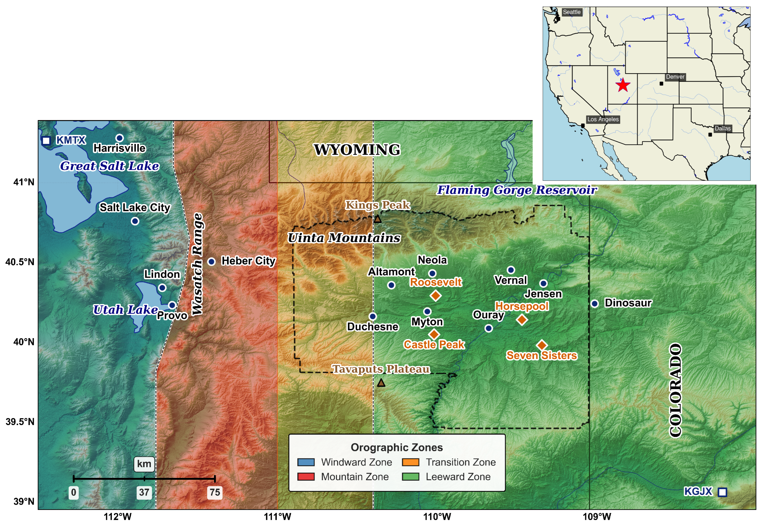
Figure 2.
A hexplot that bins observations during winter days in the observation archive for snow depth against ozone concentration. A simple linear fit (black line) shows that snowy days are also more likely to have unhealthy levels of ozone.
Figure 2.
A hexplot that bins observations during winter days in the observation archive for snow depth against ozone concentration. A simple linear fit (black line) shows that snowy days are also more likely to have unhealthy levels of ozone.
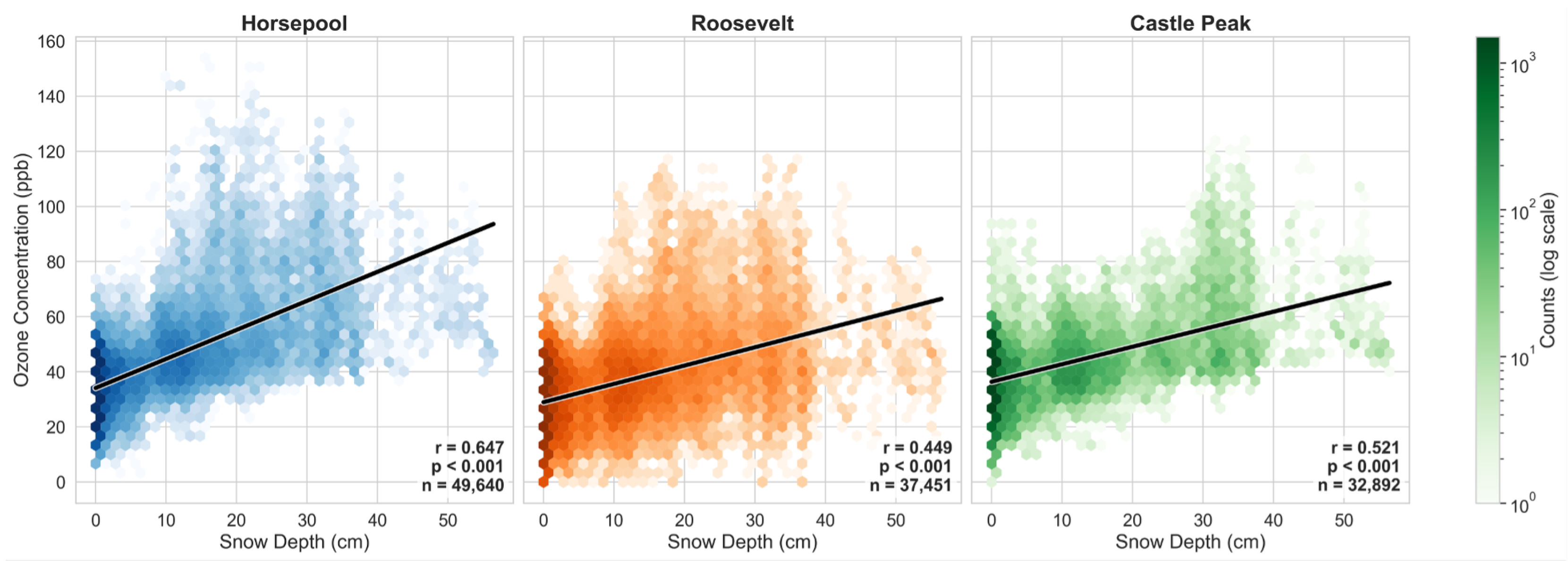
Figure 3.
Schematic of a west–east cross-section through the Uinta Basin (cf. Figure 1, where W and E in the diagram denote approximately Provo to Dinosaur, respectively) depicting the winter-ozone formation mechanism. The persistent cold pool maintains snow cover (and hence high albedo), increasing the path length for photolytic reactions to act on pollutants trapped within the cold pool. Volatile organics are abbreviated as VOs.
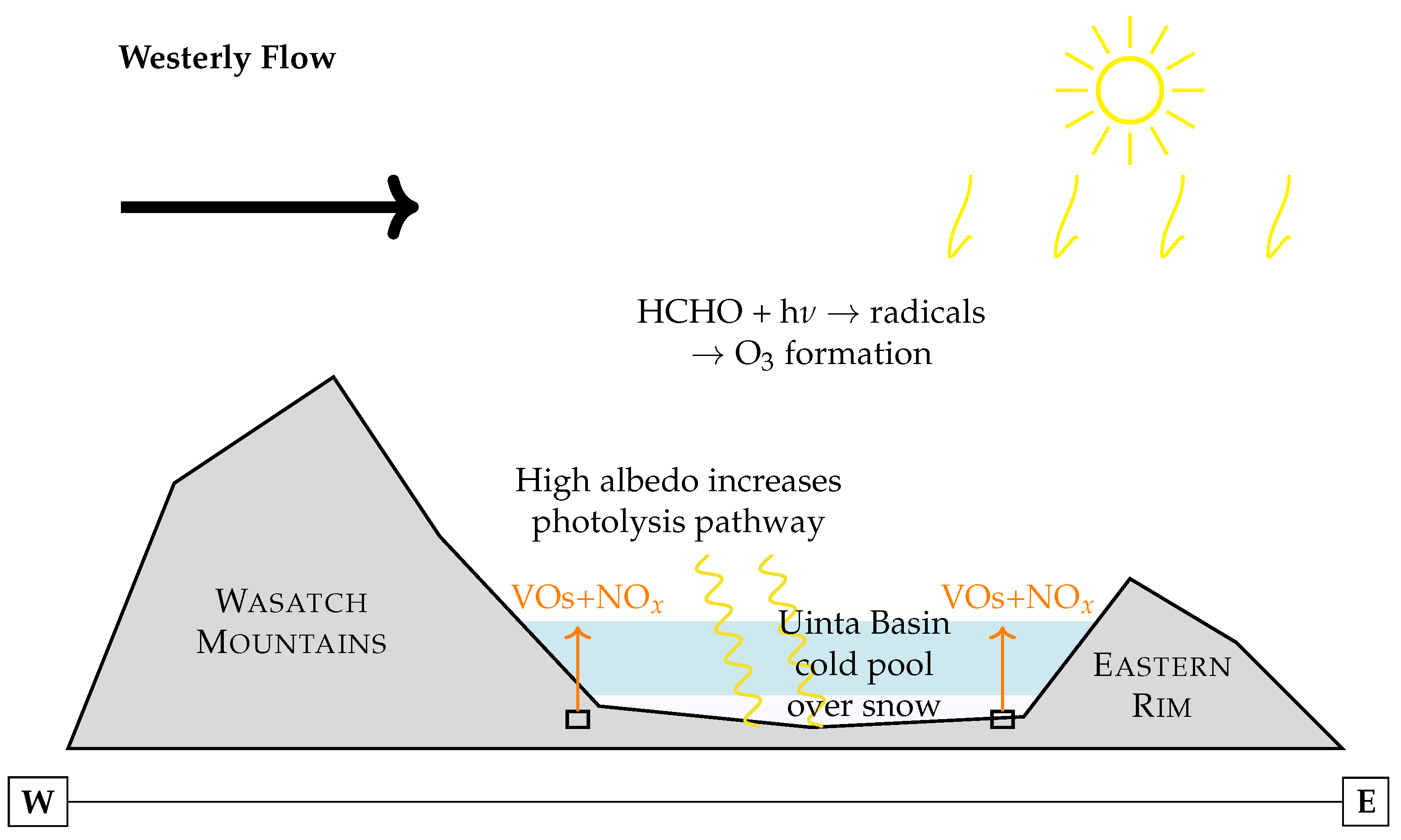
Figure 4.
Stations reporting snow depth in the Synoptic Weather database (all those ever marked `active’), locations marked with magenta cross. Towns labeled with black squares for reference in later discussion. (Also see Figure 1.)
Figure 4.
Stations reporting snow depth in the Synoptic Weather database (all those ever marked `active’), locations marked with magenta cross. Towns labeled with black squares for reference in later discussion. (Also see Figure 1.)
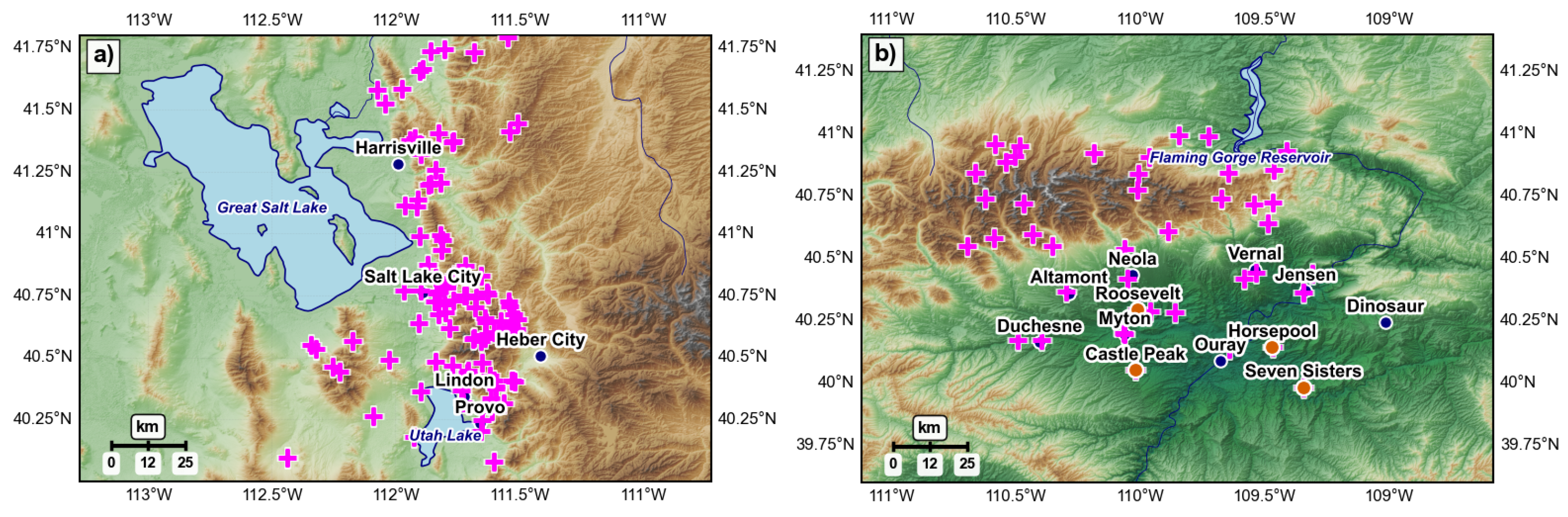
Figure 5.
Height above ground level (AGL) of the lowest three radar-beam tilts from Grand Junction (top three; KGJX) and Salt Lake City (bottom three; KMTX). NEXRAD radar locations are at the bottom right (KGJX) and top left (KMTX). The calculations shown are tilt angle at 0.2°, 0.5°, and 1.0°. The lowest 0.2°angle is permitted for these two sites [56][e.g.,][] but is evidently of little use to the Basin (located center-right in each frame). Black pixels indicate blocked radar beams from either radar site.
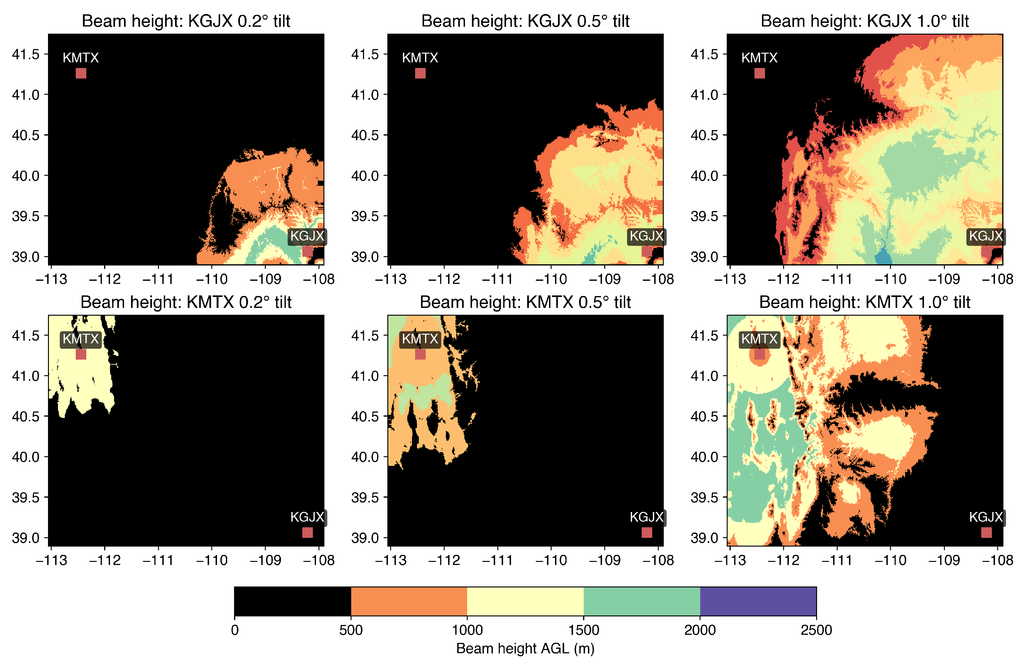
Figure 6.
Example forecasts of 8-hour maximum surface-ozone concentrations from the UFS’ AQM model. (a) The forecast initialized on 31 January 2025 (hours 4–12) shows a missed event in Basin; (b) Forecast initialized on 21 April 2025 (hours 15–23) showing elevated ozone large scale processes, likely stemming from an intrusion of stratospheric, ozone-rich air in tandem with wildfire season expanding across North America.
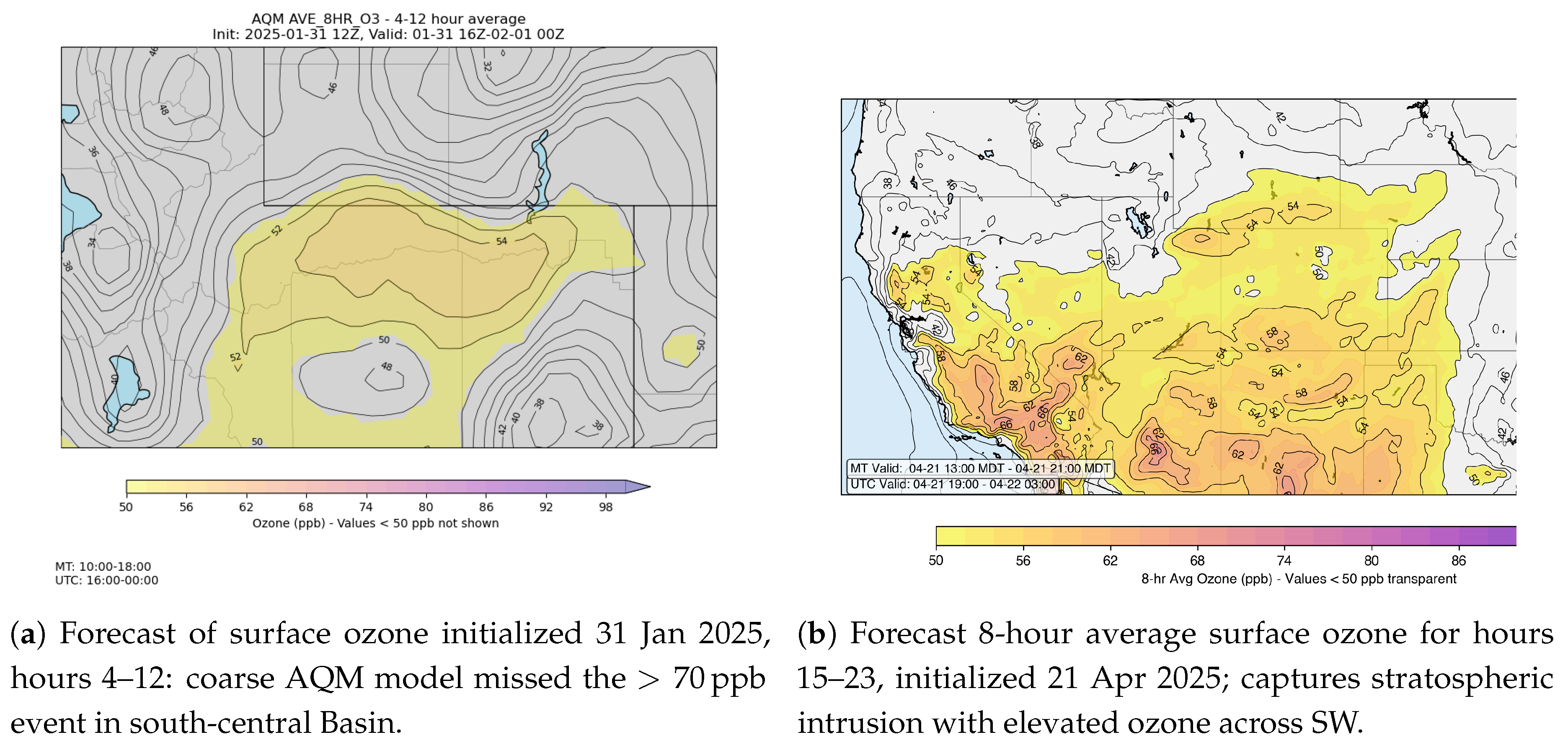
Figure 7.
Ozone concentration measured on the windward (Cooperview; Lindon; Rose Park) and leeward/Basin (Castle Peak; Horsepool; Roosevelt) side of the Wasatch Mountains for the period 0600 UTC 18 February to 0600 UTC 24 February 2023. Simulated snow cover is shown in Figure 10 during this period.
Figure 7.
Ozone concentration measured on the windward (Cooperview; Lindon; Rose Park) and leeward/Basin (Castle Peak; Horsepool; Roosevelt) side of the Wasatch Mountains for the period 0600 UTC 18 February to 0600 UTC 24 February 2023. Simulated snow cover is shown in Figure 10 during this period.
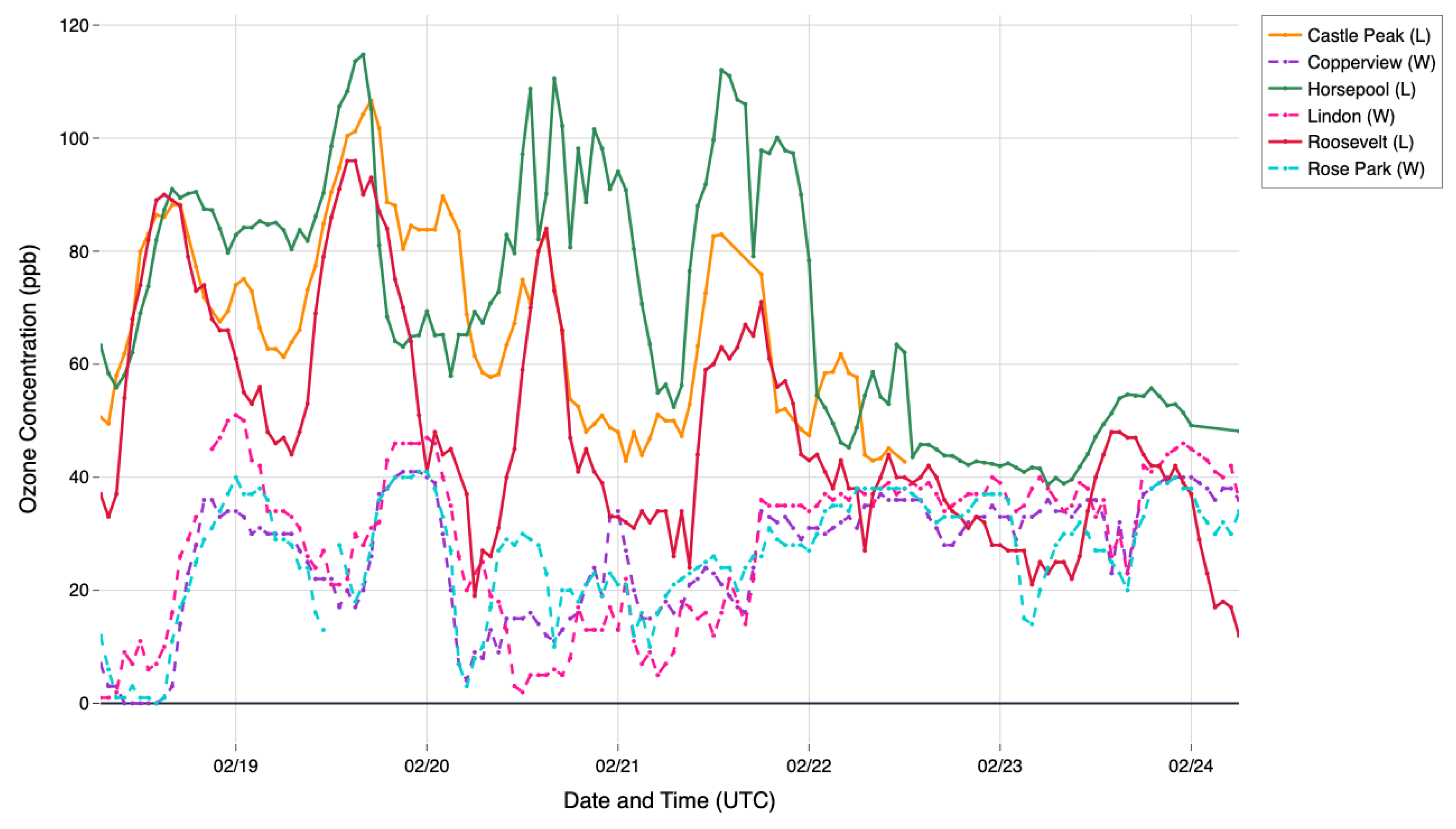
Figure 8.
Snow depth measured on the windward (Orem; Provo) and leeward/Basin (Castle Peak; Horsepool; Roosevelt) side of the Wasatch Mountains for the same period as in Figure 7.
Figure 8.
Snow depth measured on the windward (Orem; Provo) and leeward/Basin (Castle Peak; Horsepool; Roosevelt) side of the Wasatch Mountains for the same period as in Figure 7.
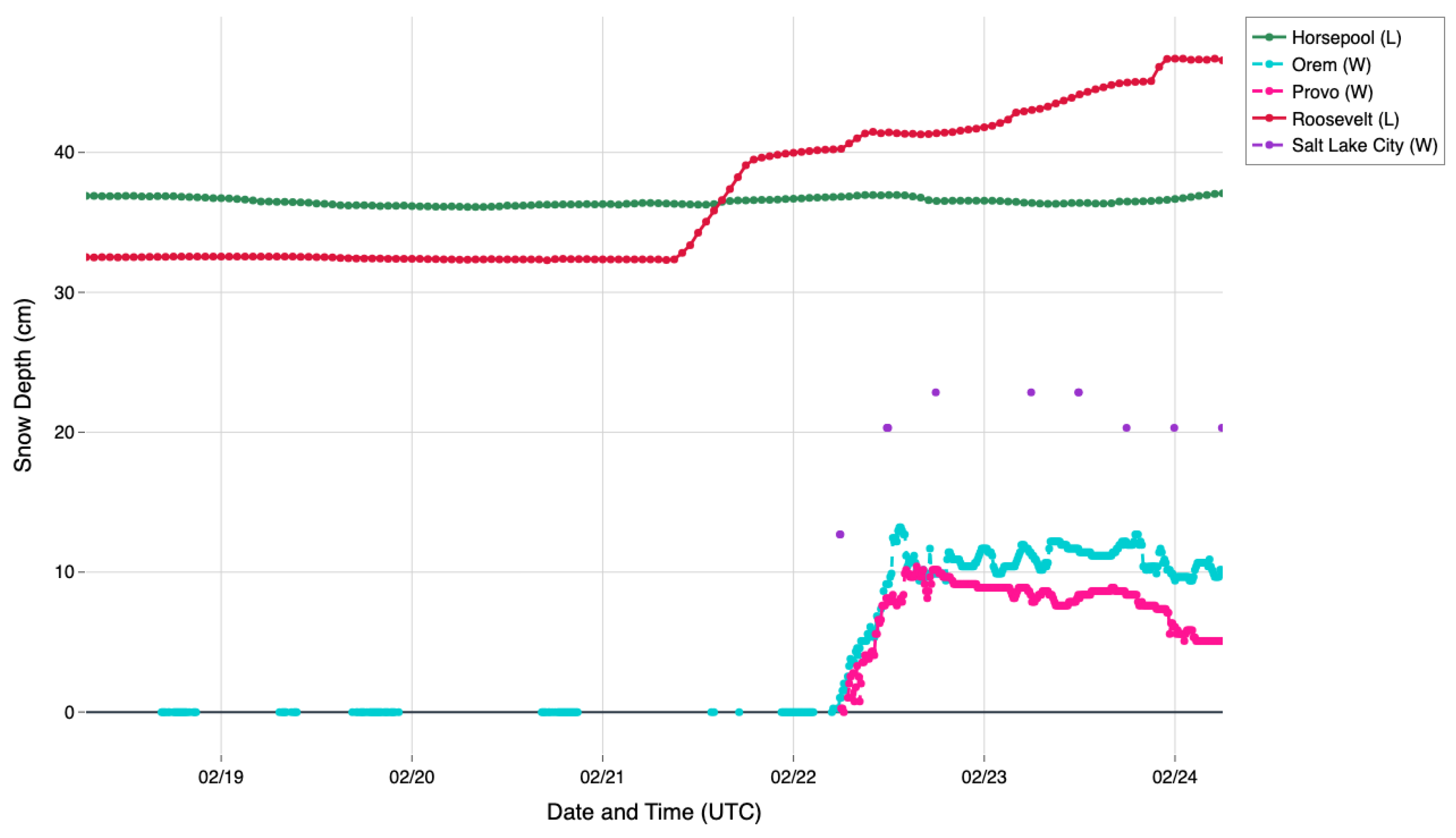
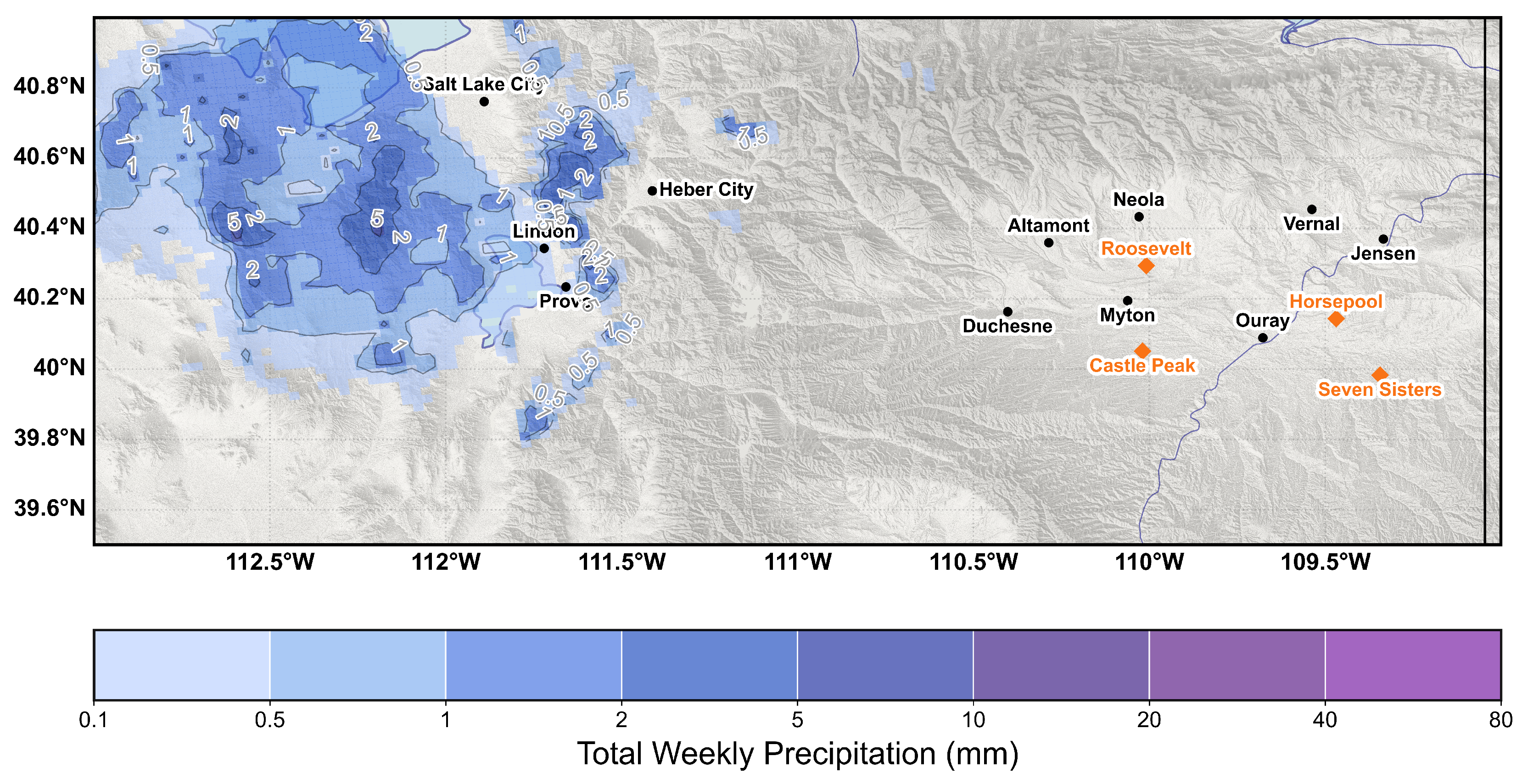
Figure 9.
Total storm precipitation (snow-water equivalent if frozen) from the RTMA gridded observation product valid roughly at the end of the study period. Snow was observed on both sides of the Wasatch Range but RTMA is unaware of much that fell across the Uinta Basin (cf. Figure 1.)
Figure 9.
Total storm precipitation (snow-water equivalent if frozen) from the RTMA gridded observation product valid roughly at the end of the study period. Snow was observed on both sides of the Wasatch Range but RTMA is unaware of much that fell across the Uinta Basin (cf. Figure 1.)
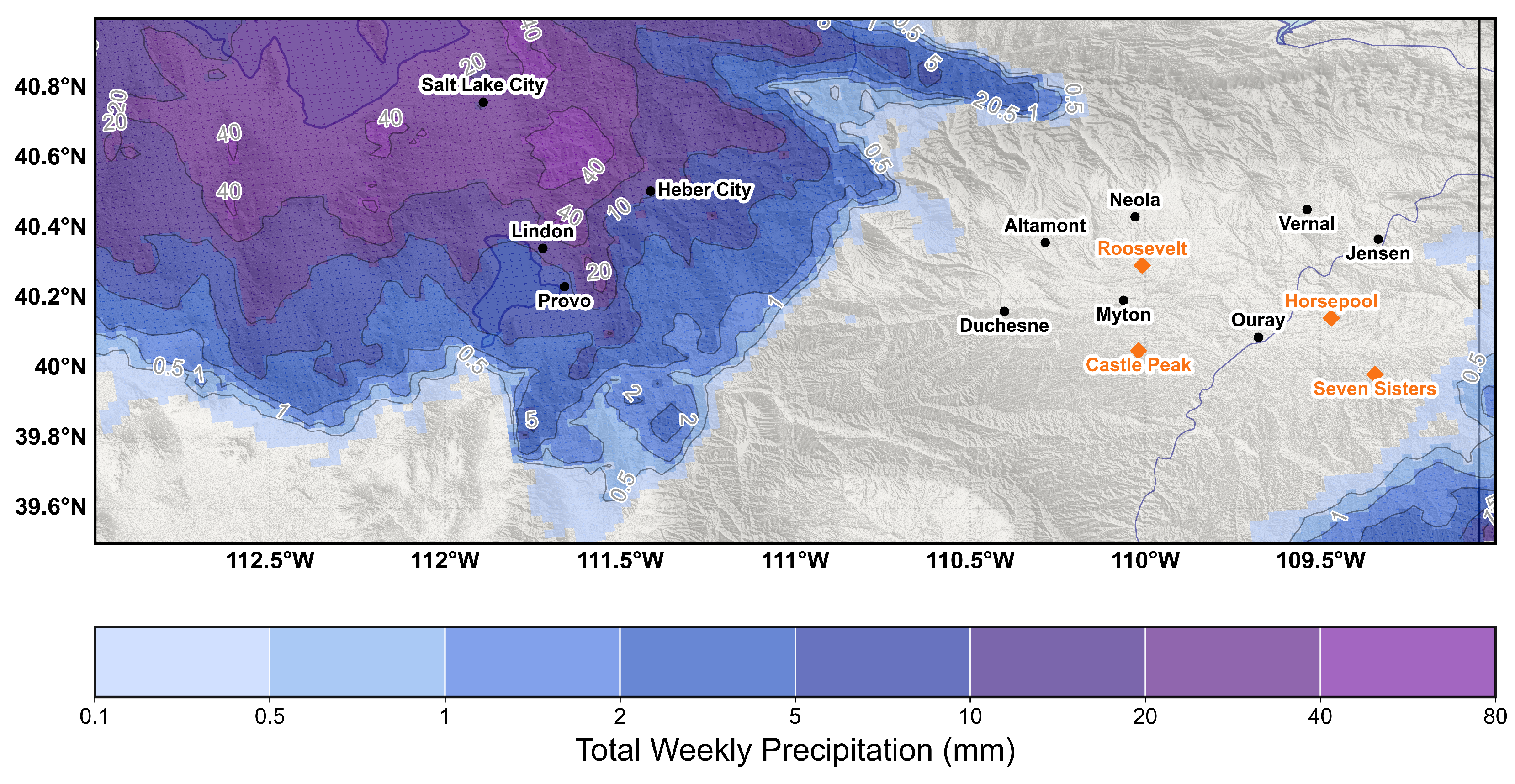
Figure 13.
Snow depth measured on leeward locations for the same period as in Figure 12.
Figure 13.
Snow depth measured on leeward locations for the same period as in Figure 12.
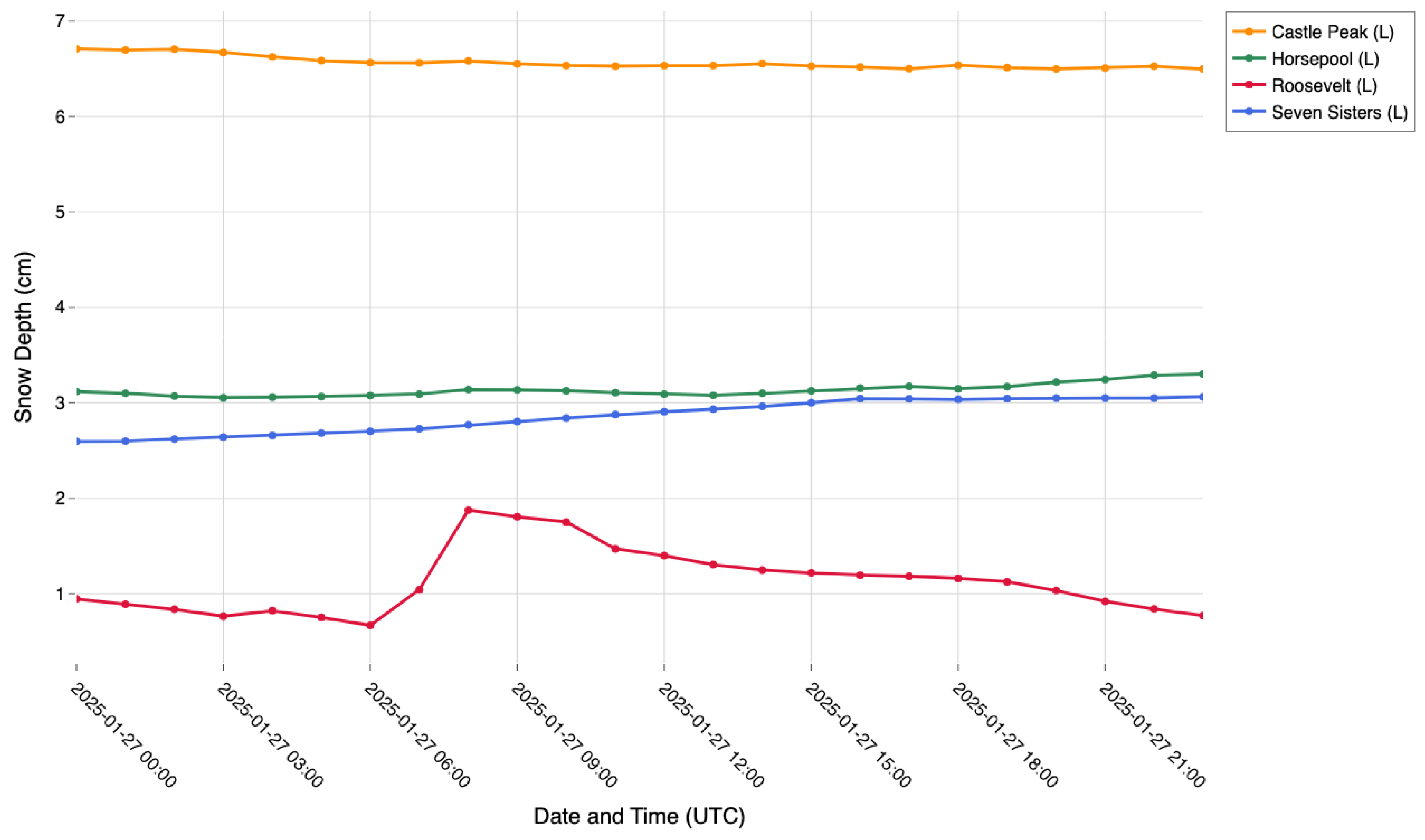
Figure 17.
HRRR analyses, initialised 1200 UTC, 27 January 2025, showing (a) 2-m dry-bulb (a) and dew-point (b) temperatures at initialization.
Figure 17.
HRRR analyses, initialised 1200 UTC, 27 January 2025, showing (a) 2-m dry-bulb (a) and dew-point (b) temperatures at initialization.
Disclaimer/Publisher’s Note: The statements, opinions and data contained in all publications are solely those of the individual author(s) and contributor(s) and not of MDPI and/or the editor(s). MDPI and/or the editor(s) disclaim responsibility for any injury to people or property resulting from any ideas, methods, instructions or products referred to in the content. |
© 2025 by the authors. Licensee MDPI, Basel, Switzerland. This article is an open access article distributed under the terms and conditions of the Creative Commons Attribution (CC BY) license (http://creativecommons.org/licenses/by/4.0/).
Copyright: This open access article is published under a Creative Commons CC BY 4.0 license, which permit the free download, distribution, and reuse, provided that the author and preprint are cited in any reuse.


