
Submitted:
12 August 2025
Posted:
13 August 2025
You are already at the latest version
Abstract
This paper presents a passive wireless temperature sensor based on an SS-compensated LC-thermistor topology. The system consists of two magnetically coupled LC tanks—each composed of a coil and a series capacitor—forming a series-series (SS) compensation network. The secondary side includes a negative temperature coefficient (NTC) thermistor connected in series with its coil and capacitor, acting as a temperature-dependent load.
Magnetically coupled resonant systems exhibit different coupling regimes: weak, critical, and strong. When operating in the strongly coupled regime, the original resonance splits into two distinct frequencies—a phenomenon known as bifurcation. At these split resonance frequencies, the load impedance on the secondary side is reflected as a pure resistance at the primary side. In the SS topology, this reflected resistance is equal to the thermistor resistance, enabling precise wireless sensing.
The advantage of the SS-compensated configuration lies in its ability to map changes in the thermistor’s resistance directly to the input impedance seen by the reader circuit. As a result, the sensor can wirelessly monitor temperature variations by simply tracking the input impedance at split resonance points. This makes the topology particularly attractive for simple, battery-free, and contactless resistive sensor (e.g thermistor) monitoring applications.
Keywords:
LC-thermistor sensor
; SS-compensation topology
; passive wireless temperature sensor
; split resonance frequencies
; resistive sensing applications
1. Introduction
Wireless passive sensors are widely employed in critical applications, including biomedical devices [1,2,3,4,5,6], harsh environment monitoring [7,8,9], structural health assessment [10,11,12], and industrial process control for temperature and pressure measurements [13,14,15,16,17]. Among various designs, LC (inductor–capacitor) topology is the most prevalent due to its cost-effectiveness and ease of implementation. Typically, the sensing side—referred to as the secondary side—comprises a capacitor usually sensitive to the target physical parameter, connected in series with an inductor. A corresponding primary coil, positioned in proximity to the sensor coil, constitutes the reader side of the system. This arrangement enables contactless sensing through magnetic coupling between the primary and secondary coils.
Although capacitors are most commonly used as the sensing element in wireless passive sensor architectures due to their straightforward integration and high sensitivity to environmental changes, alternative configurations have also been explored in the literature. In certain applications, the sensing functionality is instead provided by the inductor (coil) [18], the load resistor [19,20,21], or even the mutual inductance [22,23] between the coupled coils, which reflects the degree of magnetic coupling and varies with environmental or spatial parameters. These alternative sensing elements offer unique advantages depending on the nature of the physical parameter being monitored and the design constraints of the system. Regardless of which element is employed as the sensing component, any change in its value—caused by the variation in the measured physical quantity—results in a shift in the overall input impedance and a corresponding change in the resonance frequency of the coupled resonant circuit.
Traditionally, the primary side of a wireless LC sensor system, where the readout operation is conducted, consists solely of a single primary coil, which also serves as the defined input port. However, recent developments in wireless LC sensors have increasingly focused on enhancing sensitivity, expanding readout range, and enabling multi-parameter detection. As stated in [24], the inclusion of resonant circuitry on the primary side has led to architectures resembling magnetically coupled resonator systems, commonly used in modern wireless power transfer (WPT) applications. This approach improves both sensing performance and system integration by enabling the use of analytical tools and design strategies from the WPT domain. Building upon this concept, Zhou et al. [25] demonstrated that multi-parameter measurement can be realized using PT-symmetric dual-resonator systems, where variations in capacitance, resistance, or mutual inductance cause detectable shifts in reflection response near exceptional points (EPs). Chen et al. [26] introduced a generalized parity-time symmetric condition in RF telemetry systems with enhanced resolution and sensitivity. Dong et al. [27] advanced this concept by implementing an EP-locked wireless readout system for implantable LC microsensors.
Hajizadegan et al. [28] presented a PT-symmetric displacement sensing architecture where EP-based eigenfrequency bifurcation was exploited for high-sensitivity remote sensing. Their system enabled submillimeter displacement tracking without physical contact, using only low-cost printed coils. Zhou et al. [29] also investigated PT-symmetry breaking in LC sensors, showing that operating under a PT-asymmetric regime could effectively increase the sensing distance between the readout and sensor coils. Their approach mitigates the limitations of weak magnetic coupling, particularly relevant in sealed, miniaturized, or implantable environments. Takamatsu et al. [30] developed wearable and implantable LC bioresonators based on amplitude-modulated PT-symmetric telemetry. Their system achieved more than 2000-fold improvement in signal sensitivity and a 78% reduction in detection error for biochemical sensing of glucose and lactate concentrations, demonstrating robustness and suitability for low-power, low-volume wearable applications.
While prior studies on PT-symmetric or both-side resonant LC sensor systems have primarily emphasized eigenfrequency bifurcation, enhanced sensitivity, and multi-parameter capabilities, an essential feature intrinsic to such coupled resonator configurations—especially under series-series (SS) compensation—is often overlooked. In SS-compensated topologies, where both the reader and sensor coils are connected in series with capacitors, a key advantage emerges at the bifurcation (or split resonance) condition: the load resistance on the sensor side is precisely reflected to the input port as an equivalent input impedance [31,32,33,34,35]. This property allows for the direct and wireless readout of resistive sensing elements—such as thermistors—without the need for active electronics, making the topology exceptionally suitable for compact, battery-free, and contactless resistive sensing applications.
In this study, we exploit this characteristic by implementing a fully passive wireless temperature sensing system based on an SS-compensated LC-thermistor configuration. The sensing platform consists of two magnetically coupled and identical LC resonators, each comprising a coil and a series capacitor to form the SS topology. On the sensing side, a negative temperature coefficient (NTC) thermistor is connected in series with its LC tank, serving as a temperature-dependent resistive load. The system enables the wireless interrogation of temperature through the reflected impedance observed at the input port, leveraging the impedance mirroring behavior unique to the SS-compensated structure.
2. Mathematical Modeling of the SS-Compensated LC-Thermistor Sensor Topology
Figure 1 illustrates the circuit model of the SS-compensated LC-Thermistor topology, which consists of two magnetically coupled resonant tanks. On the primary (reader) side, an inductor Lp is connected in series with a capacitor Cp , forming a series LC circuit. On the secondary (sensor) side, another series LC circuit is formed by an inductor Ls and a capacitor Cs, which is loaded by a resistive sensing element RL. The mutual inductance M between the coils Lp and Ls enables interaction between the reader and sensor circuits. Variations in RL, due to temperature changes, influence the input impedance Zin observed at the primary side, enabling passive and contactless temperature monitoring.
The input impedance () of the SS-compensated LC sensor topology can be expressed as:
Here, denotes the impedance reflected from the secondary side to the primary, accounting for the sensor's loading effect [35]. It is derived as:
By substituting Eq. (2) into Eq. (1), a full expression for the input impedance is obtained:
To ensure optimal signal transfer between primary and secondary side, the secondary circuit is tuned to its resonance frequency:
Furthermore, in order to achieve a purely resistive input at resonance, the primary side reactance is compensated by appropriately selecting the capacitor as:
When Eq. (4) and Eq. (5) are enforced, the input impedance expression in Eq. (3) becomes more manageable, and the resonance frequencies at which the input reactance vanishes (i.e., zero-phase angle or ZPA points) can be found by setting the imaginary part of to zero [31]:
This equation always has a real solution at , provided that the primary-side compensation condition in Eq. (5) is satisfied. Additionally, two more real-valued solutions-denoted and can emerge if the following bifurcation criterion holds [31]:
The frequency consistently exists and remains invariant to the mutual inductance and load resistance , also offering a reliable operating point for sensor interrogation. In contrast, the other two ZPA frequencies only appear under the bifurcation condition and are sensitive to coupling and loading variations. The real part of the input impedance at these ZPA frequencies-commonly referred to as -can be evaluated by substituting the ZPA frequencies into Eq. (3). The solutions of , and , and bifurcation condition and are given as equations (8)-(10) in Table 1.
The input impedance, becomes pure real (Rin) at the three zero-phase angle (ZPA) resonance frequencies, , and , and is provided in Equations (11)-(13). Notably, the impedance values at and are identical, resulting in a symmetric impedance profile around in the frequency domain. These frequencies are ordered in ascending manner, where corresponds to the lowest, and to the highest resonance frequency, with located centrally between them. At depends primarily on and , while the values at and are influenced by a broader set of parameters including , and .
where
and
In practical implementations (e.g passive sensor applications as in this work), identical inductors ( and hence so capacitors (), are often used on both sides, which simplifies the analysis. In such case, the solutions of , and , and bifurcation condition and are simplified to the equations in (14)-(16) and are given in Table 2. It is important to emphasize that once the bifurcation condition is satisfied (refer to Table 2), the sensor's load resistance is effectively and directly reflected to the input impedance at the split zero-phase angle (ZPA) resonance frequencies, namely and (see Equation (17)). This direct reflection enables accurate and passive readout of the sensor resistance through impedance measurement at these specific frequencies. The presence of these split resonance frequencies offers a distinct advantage in resistive sensing applications, such as thermistor-based wireless temperature monitoring. However, practical implementation of such systems requires reliable frequency tracking mechanisms, as the useful information is encoded not only in the impedance magnitude but also in the precise location of the split resonance points on the frequency axis.

Table 2.
The solutions of , and , and bifurcation condition for identical coils (inductors).
| Solutions for ZPA Resonance Frequencies | Bifurcation Conditions |
| (14) | is real if |
| (15) | is always real |
| (16) | is real if |
3. Practical Implementation of the SS-Compensated LC-Thermistor Sensor Topology
In the experimental implementation of the LC-thermistor sensor topology, three commercially available passive components were employed to construct the resonant circuit: a planar coil, a thermistor, and a ceramic capacitor. The inductor used in both the primary and secondary resonant tanks is a flat spiral coil (model XKT-L3) with an inductance of 14 µH, an outer diameter of 43 mm, a wire diameter of 1 mm, and a thickness of 2.3 mm. Its symmetrical design ensures consistent magnetic coupling and facilitates direct reflection of the sensing resistance to the input. As the temperature-sensitive element, an NTC thermistor (model NTC10D-9) with a nominal resistance of 10 Ω at 25 °C and a 9 mm disc diameter was integrated into the secondary circuit. The thermistor’s resistance exhibits a negative exponential relationship with temperature, enabling contactless thermal sensing via changes in the system’s input impedance. For resonance tuning, a high-quality ceramic capacitor (Murata model DE1B3KX331KA4BP01F) was employed, offering an ideal capacitance value of 330 pF.
The nominal values of the aforementioned components correspond to their ideal low-frequency specifications. However, at radio frequencies (RF), these components exhibit significant parasitic behaviors—such as stray capacitance, lead inductance, skin and proximity effects, and dielectric losses—that can substantially alter their performance. As a result, accurate characterization of each component at the intended operating frequency is critical for reliable circuit design and simulation. Unfortunately, RF models or manufacturer-provided S-parameter data for the selected components were not readily available. To address this limitation, each component (coil, thermistor, and capacitor) was RF-modeled as discussed in following subsection.
3.1. RF-Modeling of Utilized Components
The components characterized as a one-port microwave network using a ROHDE & SCHWARZ ZNLE6 vector network analyzer over the 1.5 MHz to 5 MHz frequency range. Prior to measurement, a precise open-short-load (OSL) calibration was performed at the end of the measurement cable to ensure high accuracy. Figure 2 illustrates the measurement setup and shows an example of a component connected to the network analyzer during testing.
The XKT-L3 coil was first characterized through direct measurement and subsequently modeled using a three-element equivalent inductor model. This model consists of a series combination of an inductor and a resistor, both of which are in parallel with a capacitor, effectively capturing the coil’s frequency-dependent behavior at RF. The corresponding RF model and the resulting model-to-measurement fitting curves—depicting both the real and imaginary components of the input impedance—are illustrated in Figure 3(a), 3(b), and 3(c), respectively. The resistor in the model is frequency-dependent, primarily due to the skin and proximity effects that dominate at radio frequencies, and its behavior is approximated by a fitted mathematical expression, as shown in equation (19). A close match between the measurement data and the model indicates a highly accurate representation of the coil's RF behavior.
Subsequently, the capacitor was characterized using one-port S-parameter measurements obtained via the calibrated network analyzer. Analysis of the measurement results revealed that, in addition to its expected capacitive reactance, the component exhibits a frequency-dependent resistive behavior—likely due to dielectric and electrode losses increasing with frequency. To account for this, a two-element model comprising a series connection of a capacitor and a frequency-dependent resistor, of which frequency-dependency is expressed as given in equation (20), was adopted to accurately represent the RF behavior of the compensation capacitors used on both the primary and secondary sides of the circuit. The modeling results are compared with experimental data in Figure 4. As illustrated in Figure 4(b), a minor discontinuity is observed near 3 MHz that is not fully captured by the model; however, the overall agreement between the measured and simulated impedance responses is notably strong.
Finally, the thermistor is modeled using a simple two-element configuration consisting of a frequency-dependent series-connected resistor (R(f)) (see eq. (21)) and a frequency-dependent positive reactance (Z(f)) (see eq. (22)). The presence of inductive reactance is attributed to the physical structure and lead geometry of the thermistor, which introduces parasitic inductive effects under RF excitation. The modeling results are compared with the measured impedance data in Figure 5, where both the real and imaginary parts of the input impedance are shown across the frequency range of interest. As seen in Figure 5(a) and 5(b), the model closely matches the measurement data, capturing the resistive impedance variation as well as the positive slope of the imaginary component. This minimal yet effective model proves sufficient for accurately representing the thermistor’s behavior within the operating frequency range of the sensor system.
3.2. LC-Thermistor Sensor Implementation
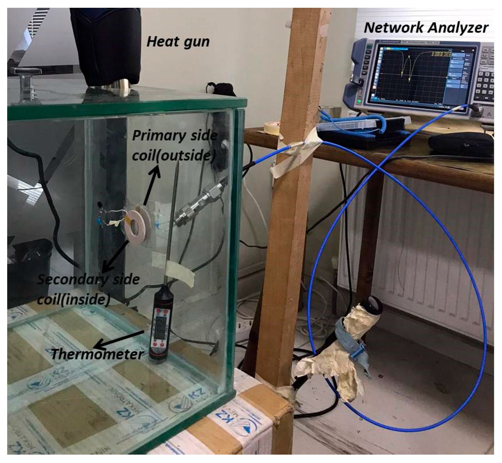
The LC-thermistor topology shown in Figure 1 was experimentally implemented in a laboratory setting. The experiments were conducted inside a cubical chamber constructed from sintered glass, designed to provide a controlled high-temperature environment. Heated airflow from a heat gun was introduced through an opening at the top of the chamber, while a thermometer placed inside enabled continuous temperature monitoring during testing.
Using this chamber, identical XKT-L3 coils and identical series-connected compensation capacitors were employed on both the primary and secondary sides, enabling direct reflection of the thermistor resistance from the sensor side to the input—forming the core operational principle of the study. The secondary side was placed inside the chamber while the primary side was outside for wireless measurement of the in-chamber temperature. The coils were precisely aligned face-to-face on opposite sides of the glass wall, separated by its 10 mm thickness. This separation resulted in a mutual inductance MMM of 3.75 µH, as determined from coupling measurements.
Figure 6.
Photograph of the experimental setup for SS-compensated LC-Thermistor sensor.
The system is configured to operate at a fundamental resonance frequency of 2.27 MHz, chosen based on the availability of off-the-shelf component values, meeting the bifurcation condition, , (see eq. (14) and (16)) and the lower frequency limit of the network analyzer used for characterization. The updated schematic, incorporating the RF models of the components described in detail above, is presented in Figure 7. At room temperature—when no heating is applied by the heat gun—the temperature inside the chamber was recorded as 25.8 °C. Under these conditions, the measured input impedance and the simulated impedance obtained using the model in Figure 7 are compared in Figure 8. As shown, the model and measurement results exhibit excellent agreement, underscoring the critical importance of accounting for the RF characteristics of the components used in the system.
As shown in Figure 8, the split resonance frequencies fL and fH, along with the system’s main resonance frequency f0, are indicated by dashed lines in both plots. These frequencies correspond to the points where the imaginary part of the input impedance crosses zero (see Figure 8b). The measured values for fL , f0, and fH are 2.045 MHz, 2.272 MHz, and 2.637 MHz, respectively.
The final stage of the laboratory experiment involved increasing the temperature inside the glass chamber using a heat gun, as illustrated in Figure 7. The temperature was gradually raised to approximately while being continuously monitored with a thermometer. Figure 9 shows the wirelessly measured input resistance () outside the chamber as a function of the in-chamber temperature at the split resonance frequencies and . At , the measured values at both and are identical, which agrees with the theoretical expectation given in Equation (17). It is important to note that the measured values include the cumulative effect of RF parasitic resistances originating from the compensation capacitors and coils. As a result, the at room temperature starts at approximately , despite the nominal thermistor load resistance being . This behavior is also evident in the model-measurement comparison plots in Figure 8(a), where the resistance values at and are clearly offset from the ideal.
As the temperature increases, the values at and diverge, creating an asymmetry around the main resonance frequency . This phenomenon is attributed to the secondary-side compensation capacitor, which is located inside the heated chamber and therefore directly exposed to temperature variations. With rising temperature, the capacitor's value shifts, introducing a perturbation [24] that alters the resonance condition of the coupled system and breaks its symmetry. Consequently, this shift causes the to either decrease by different amounts at both split frequencies or to decrease at one split frequency while increasing by a similar amount at the other. As a result, the average value of at the split frequencies,
remains very close to the value expected in a perfectly symmetric system, as shown in Figure 9. This makes also a preferred sensing parameter in scenarios where the reactive components of the circuit are subject to environmental influences such as temperature drift.
Another wirelessly measurable parameter is the input resistance at the main resonance frequency, ), whose relationship to the load thermistor resistance is given in Equation (18). As predicted by this equation, decreases as the thermistor resistance decreases with rising temperature, exhibiting an inverse proportionality between the two. This trend is clearly demonstrated in Figure 10, where a pronounced change in is observed over the tested temperature range.
An important implication of this result is the flexibility it offers in sensor readout design. While at provides a direct and simplified method of temperature measurement, the coupled resonator system inherently allows similar resistance measurements to be made at the split resonance frequencies and . Depending on the intended application and readout circuitry, the designer can choose to measure at any of these three resonance points. For example, selecting may be advantageous for single-frequency interrogation systems where circuit simplicity is critical, whereas monitoring or could provide additional sensing robustness or redundancy, particularly in environments where resonance frequency drift or asymmetry might occur. This versatility enhances the practicality of the proposed SS-compensated LCthermistor topology for a wide range of passive wireless sensing applications.
4. Discussion
The proposed SS-compensated LC-thermistor topology demonstrates a distinct advantage over conventional passive wireless sensing configurations by directly reflecting the thermistor resistance at the split resonance frequencies of the strongly coupled system. This feature, confirmed both analytically and experimentally, enables accurate, battery-free, and contactless monitoring of temperature-dependent resistance. The modeling results presented in Section 2, particularly Equations (8)–(17), show that under the bifurcation condition, two additional zero-phase-angle (ZPA) frequencies emerge symmetrically around the original resonance. This symmetry and the predictable impedance values at the split points make the topology particularly robust for resistive sensing applications.
The RF modeling of individual components (Figure 3, Figure 4 and Figure 5) played a crucial role in ensuring the accuracy of the system’s predicted performance. The extracted parameters for the inductors, capacitors, and thermistors confirmed frequency-dependent behavior that, when incorporated into the circuit model, provided excellent agreement between simulation and measurement as seen in Figure 8. The accurate representation of parasitic effects, such as series resistance and electrode-induced inductance, was essential to matching experimental outcomes with theoretical predictions.
One of the key observations from the temperature variation experiments is that secondary side compensation capacitor also varies as NTC thermistor’s resistance decreases with increasing temperature, leading to a perturbation in the coupled system that shifts the split frequencies unequally. This phenomenon, while small, suggests that environmental factors and component tolerances can induce asymmetries not accounted for in idealized models — a point also noted in earlier experimental studies of bifurcated resonance systems [24].
From an application standpoint, the ability to track sensor resistance simply by monitoring the input resistance at the split frequencies opens up promising opportunities in wireless condition monitoring. For example, the topology could be adapted for structural health monitoring by substituting the thermistor with a strain-dependent resistive sensor, or for chemical sensing using resistive films whose impedance varies with gas concentration. In addition, because the impedance mirroring effect is relatively insensitive to absolute coupling variations (as long as the bifurcation condition is satisfied), the system can tolerate moderate misalignment between reader and sensor — a significant advantage over traditional single-resonator systems.
Future research directions could focus on expanding the operational frequency range, miniaturizing the resonators for integration into compact sensor tags, and developing multi-parameter sensing schemes by combining resistive sensing with capacitive or inductive modalities in a hybrid topology. Moreover, while the current work validates the concept under laboratory conditions, field testing in realistic application environments (e.g., rotating machinery, embedded biomedical implants, or submerged monitoring stations) would further demonstrate the robustness and practicality of the approach.
5. Conclusions
This work has presented the design, modeling, and experimental validation of a passive wireless temperature sensing system based on an SS-compensated LC-thermistor topology. The system leverages the impedance mirroring property of the SS configuration to directly reflect the thermistor resistance at the split resonance frequencies, enabling accurate, battery-free, and contactless measurement. Detailed RF modeling of the constituent components ensured that the analytical predictions closely matched the measured system response. Experimental results confirmed that the topology maintains strong agreement between theoretical and practical behavior, even when accounting for frequency-dependent parasitics. Beyond temperature monitoring, the same principle could be extended to a wide range of resistive sensors, opening avenues for structural, environmental, and biomedical applications. The results suggest that the SS-compensated LC topology is a strong candidate for future low-power, high-reliability wireless sensing platforms.
Author Contributions
“Conceptualization, S.A.S.; methodology, S.A.S.; software, S.A.S. and Y.D.K.; validation, S.A.S. and Y.D.K.; formal analysis, S.A.S. and Y.D.K.; investigation, S.A.S. and Y.D.K.; resources, S.A.S. and Y.D.K.; data curation, S.A.S. and Y.D.K.; writing—original draft preparation, S.A.S.; writing—review and editing, S.A.S. and Y.D.K.; visualization, S.A.S. and Y.D.K.; supervision, S.A.S.; project administration, S.A.S.; funding acquisition, S.A.S. and Y.D.K. All authors have read and agreed to the published version of the manuscript.
References
- Moya, A.; García, C.; Vázquez, M.; Hernando, B.; Zhukova, V.; Zhukov, A. Scattering of microwaves by a passive array antenna based on amorphous ferromagnetic microwires for wireless sensors with biomedical applications. Sensors 2019, 19, 3060.
- Li, C.; Wu, J.; Yuan, H.; Yin, W.; Wang, G.; Wang, H. Overview of recent development on wireless sensing circuits and systems for healthcare and biomedical applications. IEEE J. Emerg. Sel. Top. Circ. Syst. 2018, 8, 165–177. [CrossRef]
- Huang, Q.-A.; Dong, L.; Wang, L.-F. LC passive wireless sensors toward a wireless sensing platform: Status, prospects, and challenges. J. Microelectromech. Syst. 2016, 25, 822–841. [CrossRef]
- Yeon, P.; Kim, M.-G.; Brand, O.; Ghovanloo, M. Optimal design of passive resonating wireless sensors for wearable and implantable devices. IEEE Sens. J. 2019, 19, 7460–7470. [CrossRef]
- He, D.; Cui, Y.; Ming, F.; Wu, W. Advancements in passive wireless sensors, materials, devices, and applications. Sensors 2023, 23, 8200.
- Lu, D.; Yan, Y.; Avila, R.; Kandela, I.; Stepien, I.; Seo, M.H.; Song, Y.M.; Rogers, J.A. Bioresorbable, wireless, passive sensors as temporary implants for monitoring regional body temperature. Adv. Healthc. Mater. 2020, 9, 2000942.
- Yue, W.; Yin, M.; Li, C.; Wu, Y.; Wang, Z.; Zhu, Y. Advancements in passive wireless sensing systems in monitoring harsh environment and healthcare applications. Nano-Micro Lett. 2025, 17, 106. [CrossRef]
- Tan, Q.; Wei, T.; Chen, X.; Luo, T.; Wu, G.; Li, C.; Xiong, J. Antenna-resonator integrated wireless passive temperature sensor based on low-temperature co-fired ceramic for harsh environment. Sens. Actuators A Phys. 2015, 236, 299–308. [CrossRef]
- Li, W.; Liang, T.; Liu, W.; Jia, P.; Chen, Y.; Xiong, J.; Li, Y. Wireless passive pressure sensor based on sapphire direct bonding for harsh environments. Sens. Actuators A Phys. 2018, 280, 406–412. [CrossRef]
- Wang, L.; Chen, J.; Yang, Y.; Li, Y.; Zhao, X.; Zhu, W. Passive wireless multi-parameter LC sensing system for in situ health monitoring of bearings. Sens. Actuators A Phys. 2024, 379, 115934. [CrossRef]
- Strader, N.; Jordan, B.R.; Bilac, O.; Tennant, K.M.; Reynolds, D.S.; Sabolsky, E.M.; Daniszewski, A.C. Near-field passive wireless sensor for high-temperature metal corrosion monitoring. Sensors 2024, 24, 7806. [CrossRef]
- Dong, Z.; Tu, J.; Xu, Q.; Zhu, Y.; Li, J.; Hu, Y.; Zhang, Y.; Xue, Z. A dual-sensitive element wireless passive LC temperature sensor and application in bearing monitoring. Meas. Sci. Technol. 2025, 36, 075105. [CrossRef]
- Idhaiam, K.S.V.; Caswell, J.A.; Pozo, P.D.; Sabolsky, K.; Sierros, K.A.; Reynolds, D.S.; Sabolsky, E.M. All-ceramic LC resonator for chipless temperature sensing within high temperature systems. IEEE Sens. J. 2021, 21, 19771–19779. [CrossRef]
- Varadharajan Idhaiam, K.S.; Caswell, J.A.; Pozo, P.D.; Sabolsky, K.; Sierros, K.A.; Reynolds, D.S.; Sabolsky, E.M. All-ceramic passive wireless temperature sensor realized by tin-doped indium oxide (ITO) electrodes for harsh environment applications. Sensors 2022, 22, 2165. [CrossRef]
- Lin, B.; Tan, Q.; Zhang, G.; Zhang, L.; Wang, Y.; Xiong, J. Temperature and pressure composite measurement system based on wireless passive LC sensor. IEEE Trans. Instrum. Meas. 2020, 70, 1–11. [CrossRef]
- Dutta, P.P.; Benken, A.C.; Li, T.; Ordonez-Varela, J.R.; Gianchandani, Y.B. Passive wireless pressure gradient measurement system for fluid flow analysis. Sensors 2023, 23, 2525. [CrossRef]
- Zhang, Y.; Tang, W.; Chen, H.; Li, H.; Xue, Z.; Shen, S. Flexible LC sensor array for wireless multizone pressure monitoring. IEEE Sens. J. 2023, 24, 2628–2636. [CrossRef]
- Ma, M.; Wang, Y.; Liu, F.; Zhang, F.; Liu, Z.; Li, Y. Passive wireless LC proximity sensor based on LTCC technology. Sensors 2019, 19, 1110. [CrossRef]
- Wu, T.; Bhadra, S. A printed LC resonator-based flexible RFID for remote potassium ion detection. IEEE J. Flex. Electron. 2021, 1, 47–57. [CrossRef]
- Bona, M.; Serpelloni, M.; Sardini, E.; Lombardo, C.O.; Andò, B. Telemetric technique for wireless strain measurement from an inkjet-printed resistive sensor. IEEE Trans. Instrum. Meas. 2016, 66, 583–591. [CrossRef]
- Yang, M.; Ye, Z.; Farhat, M.; Chen, P.Y. Ultrarobust wireless interrogation for sensors and transducers: A non-Hermitian telemetry technique. IEEE Trans. Instrum. Meas. 2021, 70, 1–9. [CrossRef]
- Sandra, K.R.; George, B.; Kumar, V.J. A nonintrusive magnetically coupled sensor for measuring liquid level. IEEE Trans. Instrum. Meas. 2020, 69, 7716–7724. [CrossRef]
- Al Jarrah, A.M.; Aljabarin, N. Magnetic coupling of two coils due to flow of pure water inside them–double coil volumetric flow sensor. Adv. Sci. Technol. Res. J. 2022, 16, 47–53. [CrossRef]
- Zhou, B.B.; Wang, L.F.; Dong, L.; Huang, Q.A. Observation of the perturbed eigenvalues of PT-symmetric LC resonator systems. J. Phys. Commun. 2021, 5, 045010. [CrossRef]
- Zhou, B.B.; Chen, D.; Zhang, C.; Dong, L. Realizing multi-parameter measurement using PT-symmetric LC sensors. Sensors 2024, 24, 6570. [CrossRef]
- Chen, P.Y.; Sakhdari, M.; Hajizadegan, M.; Cui, Q.; Cheng, M.M.C.; El-Ganainy, R.; Alù, A. Generalized parity–time symmetry condition for enhanced sensor telemetry. Nat. Electron. 2018, 1, 297–304. [CrossRef]
- Dong, Z.; Li, Z.; Yang, F.; Qiu, C.W.; Ho, J.S. Sensitive readout of implantable microsensors using a wireless system locked to an exceptional point. Nat. Electron. 2019, 2, 335–342. [CrossRef]
- Hajizadegan, M., Sakhdari, M., Liao, S., & Chen, P. Y. (2019). High-sensitivity wireless displacement sensing enabled by PT-symmetric telemetry. IEEE Transactions on Antennas and Propagation, 67(5), 3445-3449.
- Zhou, B.B.; Deng, W.J.; Wang, L.F.; Dong, L.; Huang, Q.A. Enhancing the remote distance of LC passive wireless sensors by parity-time symmetry breaking. Phys. Rev. Appl. 2020, 13, 064022. [CrossRef]
- Takamatsu, T.; Yu, S.; Miyake, T. Wearable, implantable, parity-time symmetric bioresonators for extremely small biological signal monitoring. Adv. Mater. Technol. 2023, 8, 2201704. [CrossRef]
- Sis, S.A. Comprehensive closed-form analysis of bifurcation in inductive wireless power transfer systems. J. Comput. Appl. Math. 2026, 473, 116847. [CrossRef]
- Thomas, E.M.; Heebl, J.D.; Pfeiffer, C.; Grbic, A. A power link study of wireless non-radiative power transfer systems using resonant shielded loops. IEEE Trans. Circ. Syst. I Regul. Pap. 2012, 59, 2125–2136. [CrossRef]
- Sis, S.A.; Kavut, S. A frequency-tuned magnetic resonance-based wireless power transfer system with near-constant efficiency up to 24 cm distance. Turk. J. Electr. Eng. Comput. Sci. 2018, 26, 3168–3180. [CrossRef]
- Sis, S.A. A circuit model-based analysis of magnetically coupled resonant loops in wireless power transfer systems. Electrica 2018, 18, 159–166.
- Wang, C.-S.; Covic, G.A.; Stielau, O.H. Power transfer capability and bifurcation phenomena of loosely coupled inductive power transfer systems. IEEE Trans. Ind. Electron. 2004, 51, 148–157. [CrossRef]
Figure 1.
Circuit model for the SS-compensated LC-Thermistor model.
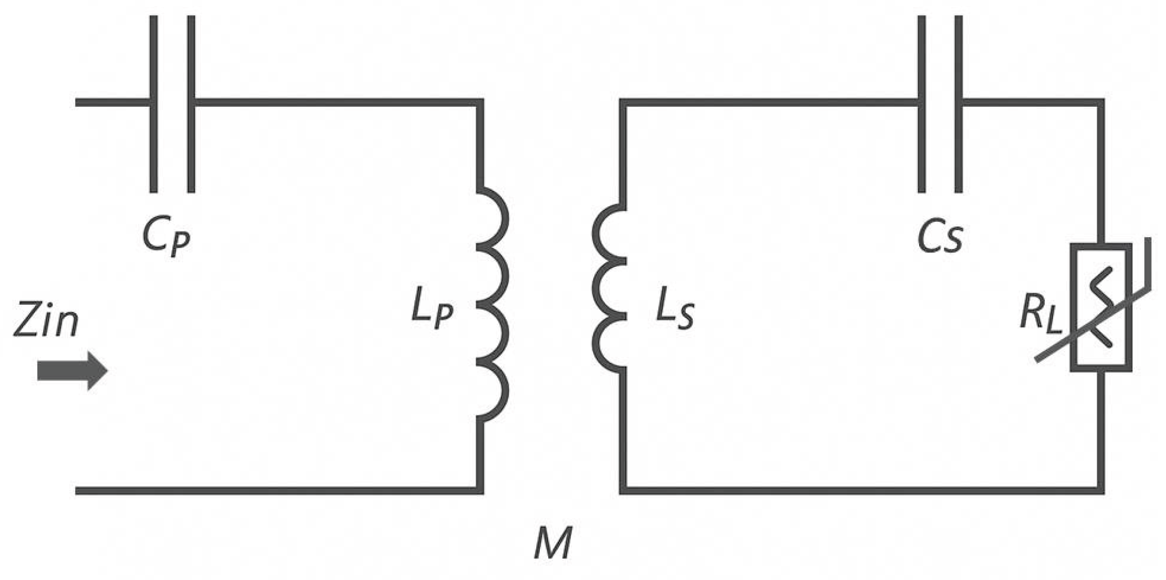
Figure 1.
Circuit model for the SS-compensated LC-Thermistor model.
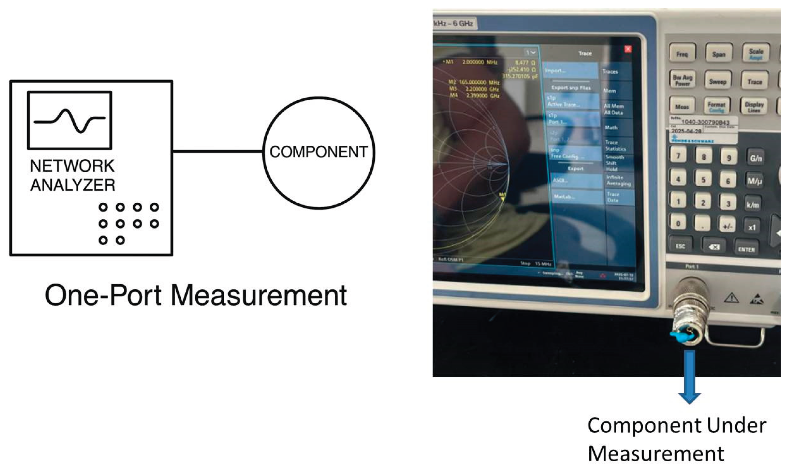
Figure 3.
(a) Equivalent RF model of the inductor based on a three-element representation. Comparison of the (b) real part and (c) the imaginary part of the input impedance obtained from the model and one-port component measurements, demonstrating strong agreement across the frequency range.
Figure 3.
(a) Equivalent RF model of the inductor based on a three-element representation. Comparison of the (b) real part and (c) the imaginary part of the input impedance obtained from the model and one-port component measurements, demonstrating strong agreement across the frequency range.
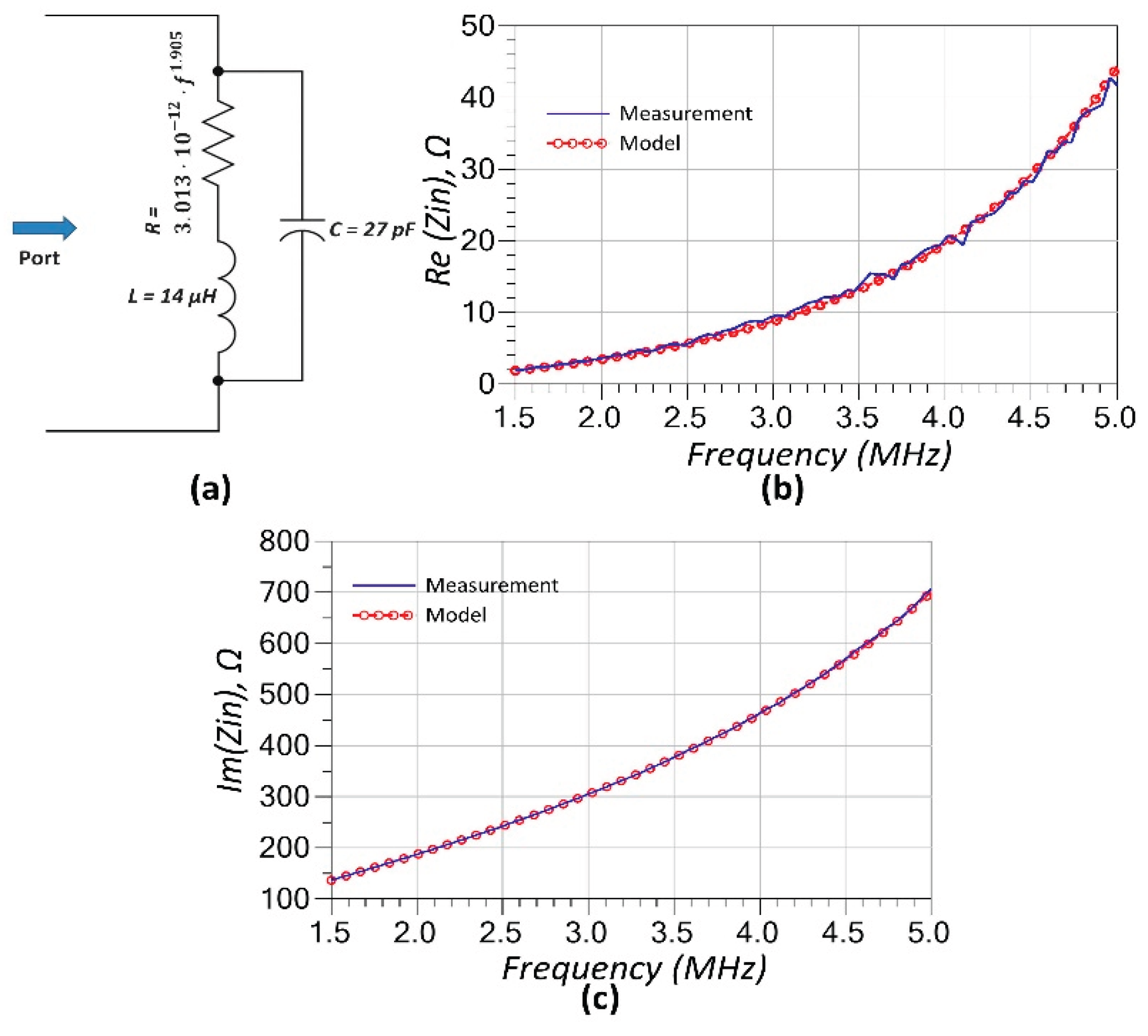
Figure 4.
(a) Equivalent RF model of the capacitor based on a two-element representation. (b) Comparison of the real part and (c) the imaginary part of the input impedance obtained from the model and one-port component measurements, demonstrating strong agreement across the frequency range.
Figure 4.
(a) Equivalent RF model of the capacitor based on a two-element representation. (b) Comparison of the real part and (c) the imaginary part of the input impedance obtained from the model and one-port component measurements, demonstrating strong agreement across the frequency range.
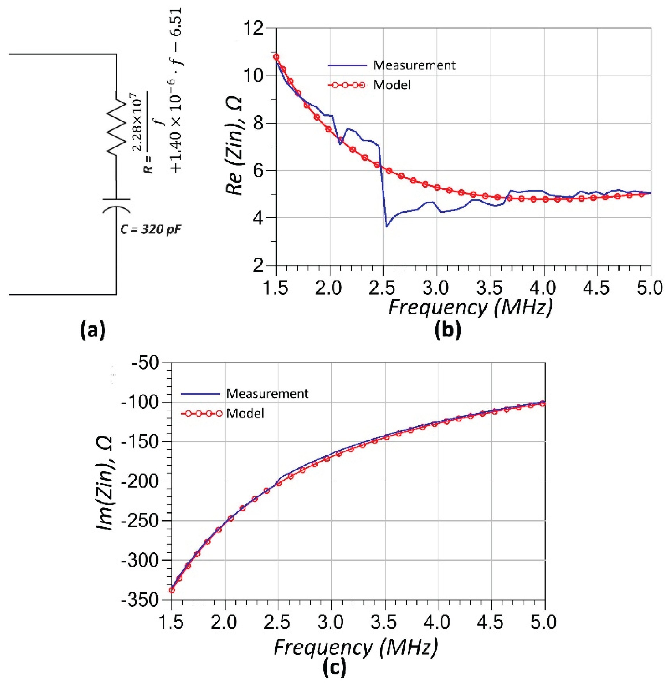
Figure 5.
(a) Equivalent RF model of the thermistor based on a two-element representation. (b) Comparison of the real part and (c) the imaginary part of the input impedance obtained from the model and one-port component measurements, demonstrating good agreement across the frequency range. The functions R(f) and Z(f) are given in equations (21) and (22).
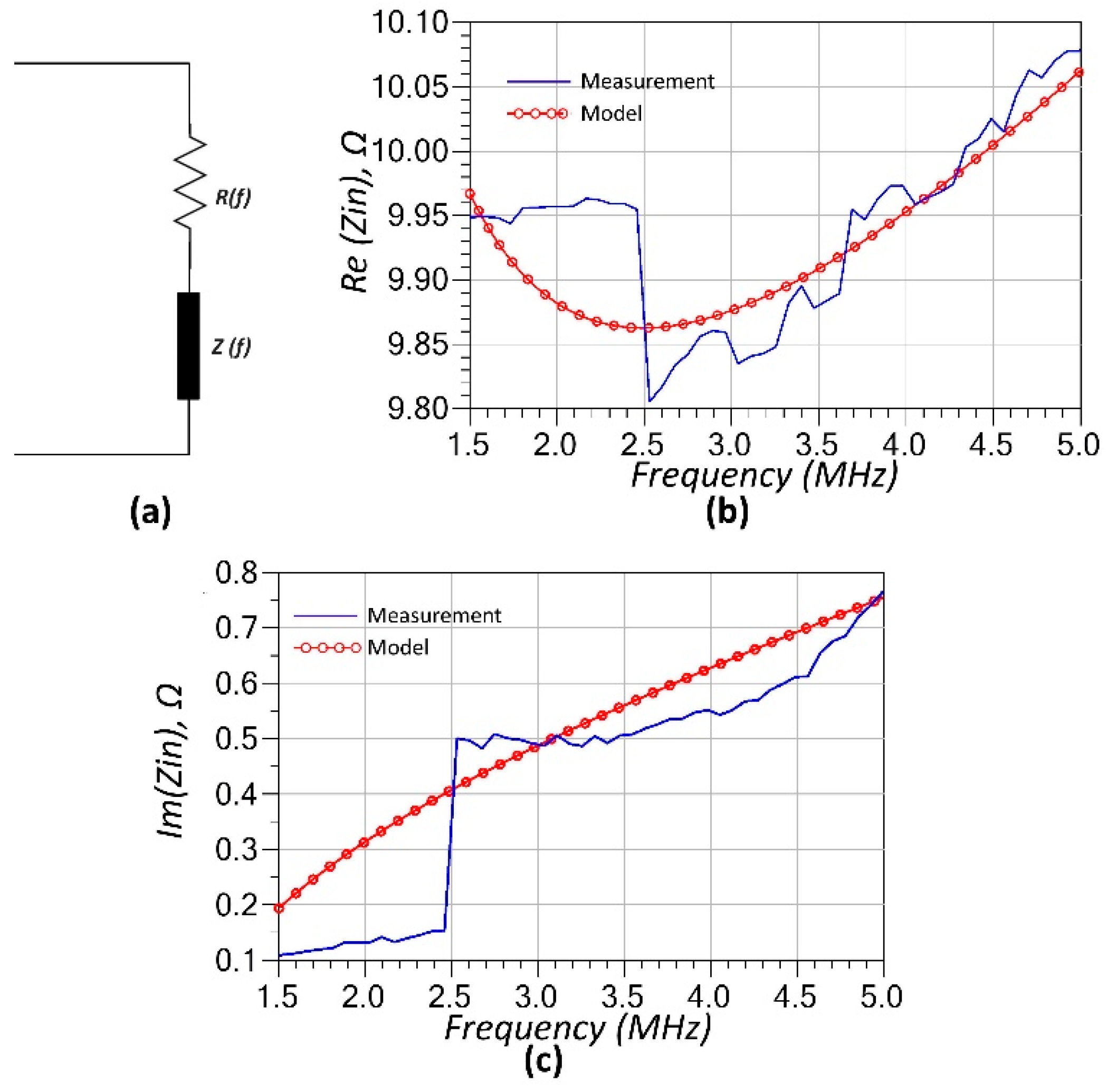
Figure 7.
Schematic of the SS-compensated LC-Thermistor with RF modeled components.
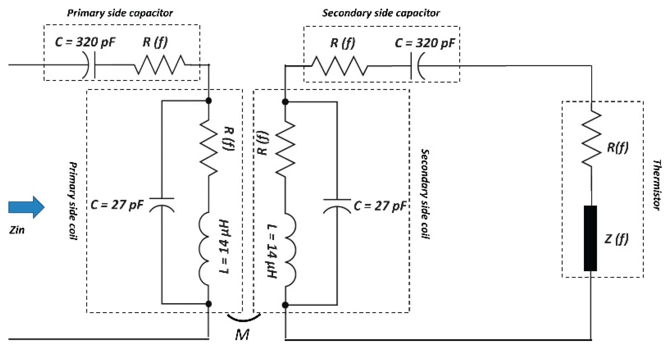
Figure 8.
Comparison of measured and simulated input impedance of SS-Compensated LC-Thermistor. (a) Real part of the input impedance (Rin) and (b) imaginary part of the input impedance (Xin) at room temperature (25.8 ⁰C).
Figure 8.
Comparison of measured and simulated input impedance of SS-Compensated LC-Thermistor. (a) Real part of the input impedance (Rin) and (b) imaginary part of the input impedance (Xin) at room temperature (25.8 ⁰C).
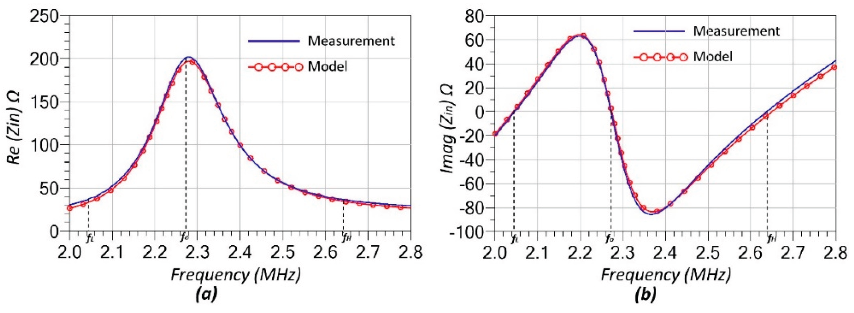
Figure 9.
Measured input resistance from input of the SS-Compensated LC-Thermistor at split resonance frequencies, fL and fH.
Figure 9.
Measured input resistance from input of the SS-Compensated LC-Thermistor at split resonance frequencies, fL and fH.
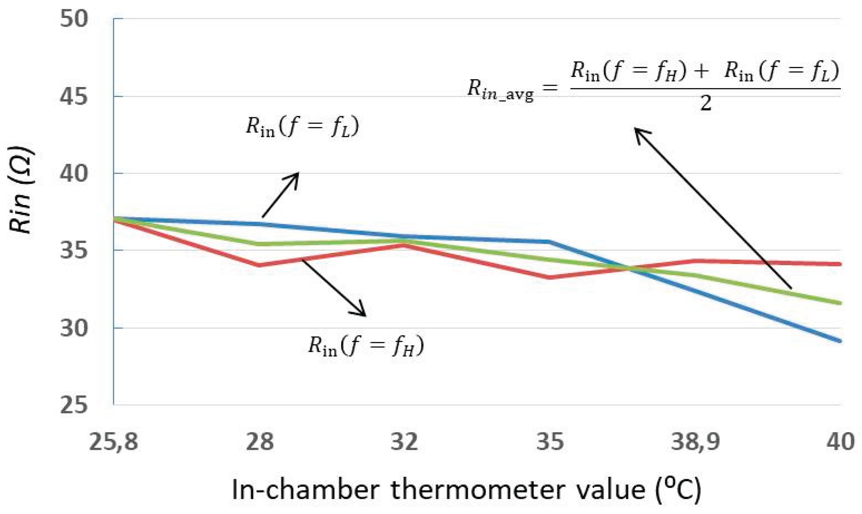
Figure 10.
Measured input resistance from input of the SS-Compensated LC-Thermistor at main resonance frequency f0.
Figure 10.
Measured input resistance from input of the SS-Compensated LC-Thermistor at main resonance frequency f0.
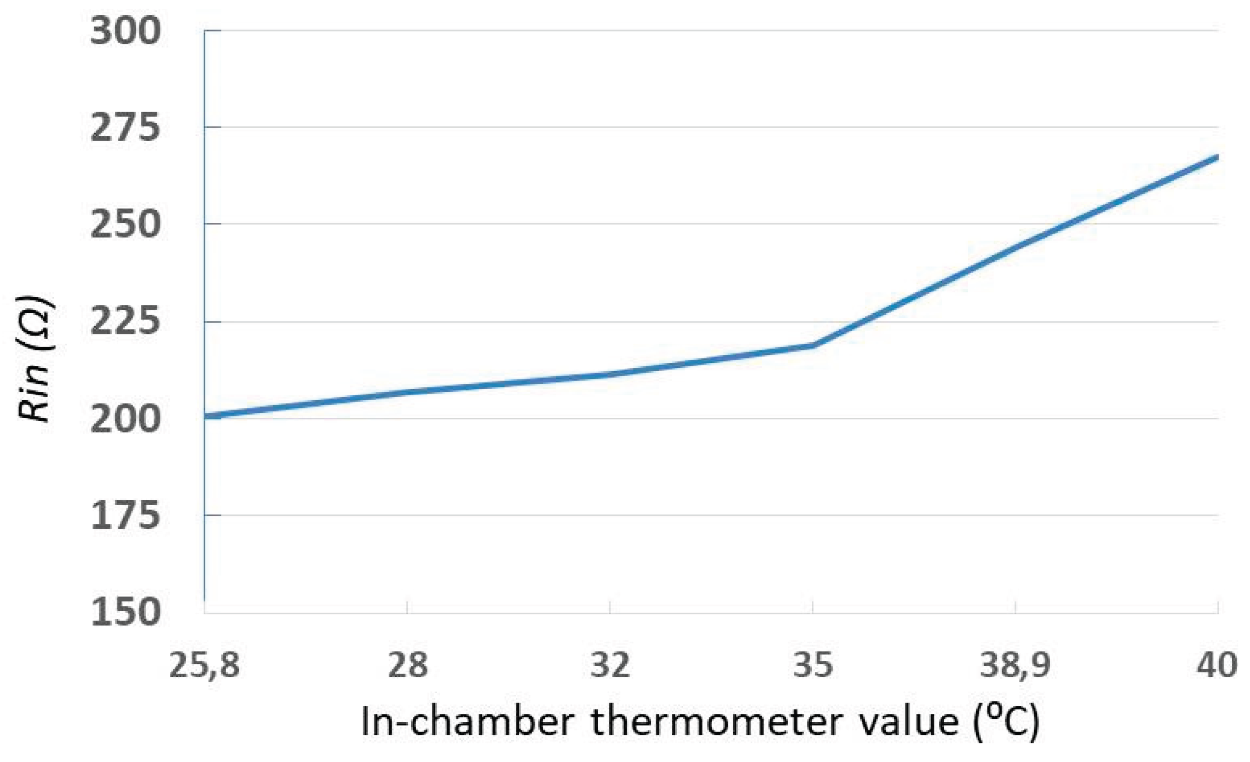
Table 1.
The solutions of , and , and bifurcation condition.
| Solutions for ZPA Resonance Frequencies | Bifurcation Conditions |
|---|---|
| (8) |
is real if |
| (9) | is always real |
| (10) |
is real if |
Disclaimer/Publisher’s Note: The statements, opinions and data contained in all publications are solely those of the individual author(s) and contributor(s) and not of MDPI and/or the editor(s). MDPI and/or the editor(s) disclaim responsibility for any injury to people or property resulting from any ideas, methods, instructions or products referred to in the content. |
© 2025 by the authors. Licensee MDPI, Basel, Switzerland. This article is an open access article distributed under the terms and conditions of the Creative Commons Attribution (CC BY) license (http://creativecommons.org/licenses/by/4.0/).
Copyright: This open access article is published under a Creative Commons CC BY 4.0 license, which permit the free download, distribution, and reuse, provided that the author and preprint are cited in any reuse.


